Using stochastic computation graphs formalism
for optimization of sequence-to-sequence model

Abstract

Variety of machine learning problems can be formulated as an optimization task for some (surrogate) loss function. Calculation of loss function can be viewed in terms of stochastic computation graphs (SCG). We use this formalism to analyze a problem of optimization of famous sequence-to-sequence model with attention and propose reformulation of the task. Examples are given for machine translation (MT). Our work provides a unified view on different optimization approaches for sequence-to-sequence models and could help researchers in developing new network architectures with embedded stochastic nodes.

1 Introduction

Stochastic computation graph is a directed acyclic graph which includes both deterministic nodes and conditional probability distributions [Schulman et al., 2015]. Leaves of the computation graph are cost nodes whose sum can be attributed to total loss function of a machine learning model. By taking the expectation of sum of cost nodes w.r.t. random variables we receive expected loss. Having defined loss function as mathematical expectation of costs calculated by SCG, we can view losses for many seemingly different problems in a uniform way:

$$L(x,y_{true},\theta,\theta^{\prime})=\mathbb{E}_{z\sim p(z;\theta)}\sum_{c\in\mathcal{C}}c(x,y_{true},z,\theta^{\prime})$$ (1)

Here $x$ are inputs, $y_{true}$ are corresponding ground-truth outputs, $z$ are random variables with probability distributions parameterized by $\theta$, $\theta^{\prime}$ are other parameters of a model. $\mathcal{C}$ is a set of cost nodes, $c$. We refer reader to the seminal article [Schulman et al., 2015] where authors provide examples of such reformulation for reinforcement learning (RL) problem setup and generative models.

Once we casted loss function as an expectation of costs calculated by SCG, we need to calculate its derivatives in order to use effective gradient-based approaches for optimization. Given that parameters of the model may be included in both probability distributions and deterministic non-linear transformations, the task of calculating the gradient may become problematic:

1. Closed analytical formula for gradient usually cannot be derived, and even formulae that include expectations are cumbersome.

2. If computation of gradient involves taking integrals numerically, samples often show large variance.

As for the first problem, there is a general formula [Schulman et al., 2015] which can be considered as a generalization of the well-known REINFORCE rule [Williams, 1992] and the usual backpropagation algorithm for deterministic computation graphs. It provides a straightforward way to obtain an unbiased estimate of the gradient of loss function by approximating expectations with Monte-Carlo samples. This is where the second problem comes to play. Naive numerical calculation of gradient may fail because of large variance of samples and some additional tricks are needed to make the procedure more sample-efficient: control variates [Greensmith et al., 2004], common random numbers etc.

Recently, reparameterization trick for continuous distributions [Kingma and Welling, 2013] has become popular for the same purposes and a similar procedure [Jang et al., 2016, Maddison et al., 2016] was developed for discrete distributions. In the latter case, we introduce bias in gradient estimate but decrease the variance.

Stochastic computation graphs provide a convenient framework for the analysis of machine learning models. It also encourages us to use general variance reduction techniques for Monte-Carlo integration, not restricting ourselves to some "practices" which are common in fields where similar problems occur (such as baselines for lowering variance of score function estimator in RL).

The contributions of this work are as follows:

1. Re-formulation of an example NLP model using the SCG formalism, thus describing different optimization approaches in common terms.

2. Analysis of the existing training procedures for this model using the SCG formalism.

3. Testing different variance reduction techniques for the efficient optimization of the model.

2 Sequence-to-sequence model

Sequence-to-sequence architectures (seq2seq) are a wide class of models that produce a sequence of tokens from an arbitrary input. Some examples of their applications are machine translation [Sutskever et al., 2014], summarization [Rush et al., 2015].

Widely used approach to training of seq2seq models is maximizing the likelihood of each successive target token conditioned on the input sequence and the history of target tokens. This approach is known as teacher forcing [Williams and Zipser, 1989] and is illustrated on Figure 1. Although proved to be effective in practice, at test time it does not give model the access to correct tokens, but only to its own predictions. Hence inference procedure is different at training and test time. This leads to two major issues [Wiseman and Rush, 2016]:

1. Exposure bias. Model is not exposed to its own outputs during training.

2. Loss-evaluation mismatch. During training we optimize a differentiable metric, but measure quality with another metric (such as BLEU [Papineni et al., 2002]).

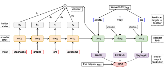
Figure 1: An example of sequence-to-sequence model with attention. Calculation of cross-entropy loss function with teacher forcing is shown. <BOS> is a token that denotes start of a sentence. All nodes in the graph are calculated deterministically and denoted by rounded rectangles.

Several approaches have been developed in order to mitigate these issues.

One is alternating regime of "scheduled sampling" [Bengio et al., 2015] where model can receive either inputs from target sequences or samples from the output distribution at different training steps randomly. Log likelihood of correct labels is optimized. This method is developed within supervised learning paradigm (cases A and B in Figure 2.

Second approach is to consider sampling from output distribution as an agent’s action, thus considering the task in RL paradigm (case C in Figure 2). Because of that, direct optimization of target non-differentiable metric can be performed using RL techniques [Paulus et al., 2017].

In our opinion, there is nothing conceptually different between these approaches. They can be unified if we define loss function of seq2seq model in stochastic graph formalism as in Figure 2. Then the expectation in equation  1 corresponds to sampled words from output distributions. We can consider these intermediate outputs as latent variables which are marginalized to get loss function depending only on external data and parameters of a model. Given general formula [Schulman et al., 2015] for an unbiased estimate of gradient of corresponding loss, we now focus on its practical (i.e. data) efficiency.

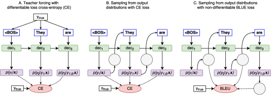
Figure 2: Different approaches to optimization of seq2seq model. For brevity, only decoder part is shown, encoder is the same as on Figure 1. Circles denote stochastic nodes where sampling is performed. A. Usual teacher forcing approach. B. Outputs from previous step are sampled and fed at the next time step. C. Same as in case B, but a non-differentiable metric is being optimized.

3 Results and discussion

We optimized all three losses shown in Figure 2 in common SCG framework for MT task. The results are given in Table 1 in the form "mean $\pm$ std". We performed 5 runs for each experiment in order to compute standard deviation. For the approach B ("feed samples"), when outputs from the previous step are sampled and fed at the next time step, we tested three different approaches to optimization. For all experiments we used early stopping (computation stops when loss on validation set stop decreasing, approximately between 10000-th and 20000-th batch), except for direct BLEU optimization, when we stopped after 100000 batches, not waiting for model to start overfitting. For direct optimization of BLEU (approach C on Figure 2) control variates as a variance reduction technique were implemented.

The choice of model architecture was motivated by a compromise between simplicity (to allow fast experiments) and representativity (to ensure results are transferable). Same model as in [Wiseman and Rush, 2016] was used: single-layer bidirectional LSTM encoder and single-layer LSTM decoder with multiplicative attention mechanism [Luong et al., 2015]. Hidden dimension of LSTM cells is 256 and pretrained fasttext embeddings [Bojanowski et al., 2016] of size 300 were used for initialization. We used Adam [Kingma and Ba, 2014] with learning rate 0.001 when optimizing cross-entropy, and with learning rate 0.0001 when directly optimizing BLEU. We trained our models on dataset is IWSLT’14 dataset [Cettolo et al., 2014] of German-English sentence pairs.

Table 1: Experimental results for MT. Either differentiable loss function Cross-Entropy (CE) was used or we directly optimized the target BLEU metric (last line).

	CE loss		BLEU
	train	eval (best)	train	eval (best)
Teacher-forcing (Figure 2A, CE opt.)	$5.96\pm 0.03$	$6.44\pm 0.08$	$31.8\pm 4.9$	$19.6\pm 3.6$
Feed samples (Figure 2B, CE opt.):
naive gradient	$3.41\pm 0.17$	$4.20\pm 0.10$	$20.1\pm 2.7$	$9.8\pm 1.3$
full gradient, control variates	$3.45\pm 0.23$	$4.24\pm 0.08$	$12.4\pm 1.7$	$8.0\pm 0.7$
full gradient, Gumbel reparam.	$3.43\pm 0.16$	$4.22\pm 0.07$	$16.8\pm 1.5$	$8.7\pm 0.3$
full gradient (Figure 2C, direct BLEU opt.)	-	-	$24.6\pm 0.1$	$22.0\pm 0.2$

Let us now discuss differences between training procedures for loss functions shown in Figure 2. Teacher forcing case is trivial: there are no non-differentiable or stochastic nodes in the graph, so usual backpropagation algorithm works fine.

If we introduce additional stochastic nodes in the graph, then in order to get an unbiased estimate for the gradient of loss function we need to backpropagate through stochastic nodes; the gradient consists of two terms in this case: the first one that flows through by all the paths in the graph that go through stochastic nodes, and the second one, that is just usual backpropagation term. We do not reproduce all the formulae here, they can be found in [Schulman et al., 2015]. Hereinafter we refer to the sum of these two terms as "full" gradient, and just the second term is referred to as "naive" gradient.

For scheduled sampling, authors of [Bengio et al., 2015] used naive gradient to train a model. It resulted in a biased estimate of gradient. One of the stimulating questions for the present work was to clarify how optimization process would change once we start using unbiased gradient estimates (but probably with larger variance).

Introducing stochastic nodes allows us to optimize non-differentiable metrics, because in this case the expression for the full gradient does not include derivatives of cost nodes ("score function" estimator [Schulman et al., 2015]). As an illustrative example, we do not need a model of environment when using policy gradient theorem [Sutton et al., 2000] in RL just because of this. This is why one appeals to RL optimization procedures, once a non-differentiable metric occurs. As a price to pay, this estimator shows large variance [Greensmith et al., 2004]. In our opinion, the whole RL machinery seems to be a bit redundant here, because we do not actually need to define of "agent", "environment" (or Markov decision process) here. We can just consider an arbitrary graph with stochastic nodes and optimize a corresponding loss function.

To summarize, there are three most common approaches to optimize loss functions represented as SCG:

1. Naive gradient (ignore paths through stochastic nodes): applicable to cases A and B on Figure 2. Cannot be applied to case C, because loss function is non-differentiable.

2. Full gradient: universal, for case A in Figure 2 reduces to naive gradient.

3. Reparameterization trick: case B in Figure 2. Same as naive gradient, cannot be applied to case C.

The latter approach can introduce bias in gradient estimate (for example, if we use reparameterization for discrete distributions [Jang et al., 2016]), but usually greatly reduces variance. In this case we actually change computation graph, but do not change expected loss.

4 Conclusions

SCG formalism provides a convenient framework for the analysis of machine learning architectures by showing assumptions made in corresponding approaches explicitly. Also, adding new stochastic nodes (i.e. hard attention mechanism [Xu et al., 2015] instead of soft one) does not cause change in training paradigm from "supervised learning" to "reinforcement learning". SCG formalism allows to get rid of seemingly different approaches to the same task and review it from a common perspective.

Using sampling can be viewed as regularization technique: that is, comparing teacher-forcing and sampling approaches, we observed that the latter approach results in smaller margin between metrics on train and validation sets.

Using full gradient instead of naive one didn’t provide any advancement in evaluation metrics in our experiments. This is likely due to high variance of gradient estimate. One way to mitigate it is to use better control variate (a promising example: [Tucker et al., 2017]), that remains a subject for future work.

Acknowledgments

This work was supported by National Technology Initiative and PAO Sberbank project ID 0000000007417F630002.

References

- [Bengio et al., 2015] Bengio, S., Vinyals, O., Jaitly, N., and Shazeer, N. (2015). Scheduled sampling for sequence prediction with recurrent neural networks.
- [Bojanowski et al., 2016] Bojanowski, P., Grave, E., Joulin, A., and Mikolov, T. (2016). Enriching word vectors with subword information.
- [Cettolo et al., 2014] Cettolo, M., Niehues, J., Stuker, S., Bentivogli, L., and Federico, M. (2014). Report on the 11th iwslt evaluation campaign, iwslt 201.
- [Greensmith et al., 2004] Greensmith, E., Bartlett, P. L., and Baxter, J. (2004). Variance reduction techniques for gradient estimates in reinforcement learning.
- [Jang et al., 2016] Jang, E., Gu, S., and Poole, B. (2016). Categorical reparameterization with gumbel-softmax.
- [Kingma and Ba, 2014] Kingma, D. P. and Ba, J. (2014). Adam: A method for stochastic optimization.
- [Kingma and Welling, 2013] Kingma, D. P. and Welling, M. (2013). Auto-encoding variational bayes.
- [Luong et al., 2015] Luong, M.-T., Pham, H., and Manning, C. D. (2015). Effective approaches to attention-based neural machine translation.
- [Maddison et al., 2016] Maddison, C. J., Mnih, A., and Teh, Y. W. (2016). The concrete distribution: A continuous relaxation of discrete random variables.
- [Papineni et al., 2002] Papineni, K., Roukos, S., Ward, T., and Zhu, W.-J. (2002). Bleu: a method for automatic evaluation of machine translation.
- [Paulus et al., 2017] Paulus, R., Xiong, C., and Socher, R. (2017). A deep reinforced model for abstractive summarization.
- [Rush et al., 2015] Rush, A. M., Chopra, S., and Weston, J. (2015). A neural attention model for abstractive sentence summarization.
- [Schulman et al., 2015] Schulman, J., Heess, N., Weber, T., and Abbeel, P. (2015). Gradient estimation using stochastic computation graphs.
- [Sutskever et al., 2014] Sutskever, I., Vinyals, O., and Le, Q. V. (2014). Sequence to sequence learning with neural networks.
- [Sutton et al., 2000] Sutton, R. S., McAllester, D., Singh, S., and Mansour, Y. (2000). Policy gradient methods for reinforcement learning with function approximation.
- [Tucker et al., 2017] Tucker, G., Mnih, A., Maddison, C. J., Lawson, D., and Sohl-Dickstein, J. (2017). Rebar: Low-variance, unbiased gradient estimates for discrete latent variable models.
- [Williams, 1992] Williams, R. J. (1992). Simple statistical gradient-following algorithms for connectionist reinforcement learning.
- [Williams and Zipser, 1989] Williams, R. J. and Zipser, D. (1989). A learning algorithm for continually running fully recurrent neural networks.
- [Wiseman and Rush, 2016] Wiseman, S. and Rush, A. M. (2016). Sequence-to-sequence learning as beam-search optimization.
- [Xu et al., 2015] Xu, K., Ba, J., Kiros, R., Cho, K., Courville, A., Salakhutdinov, R., Zemel, R., and Bengio, Y. (2015). Show, attend and tell: Neural image caption generation with visual attention.