Abstract

The study of nuclear and subnuclear structure by means of photon scattering is outlined. Besides a brief exposition of the formalism a few illustrative examples are discussed.

Chapter 0 Photon Scattering off Nuclei^∗

1 Introduction

I would like to begin with a brief personal remark: It was during the fall of 1964 - I just had completed my diploma thesis in experimental physics at the University of Freiburg - , when Walter Greiner offered me to work on a PhD thesis in his new established theory group at the University of Frankfurt. As subject of the thesis he had proposed to investigate the structure of heavy deformed nuclei in the region of the giant resonances by means of photon scattering. By the end of 1965 Hans-Jürgen Weber and myself were Walter’s first PhD-students to complete their PhD. Since then, my interest in the study of electromagnetic reactions on nuclei in general, e.g. photo absorption and scattering, electron scattering and meson production, has continued up to present times.

Electromagnetic reactions on nuclei provide an excellent tool to investigate nuclear structure. In addition, they also lead to valuable insights into the electromagnetic properties of the nuclear constituents, proton and neutron, like for example, electric and magnetic polarizabilities and electromagnetic form factors. In this context photon scattering experiments are a particularly interesting source of information on off-shell properties of the nuclear constituents. On the other hand genuine microscopic calculations of photon scattering cross sections are rather complicated since in principle the complete excitation spectrum has to be taken into account.

Here I will give a brief account of photon scattering reactions on nuclei with emphasis on my own work and that of my collaborators. It is not intended as a general review, rather a personal view on this interesting reaction which over many years has fascinated myself and which was and still is subject of my own research. Early reviews on nuclear photon scattering may be found in Refs. 1, 2, 3 and a more recent one in Ref. 4.

In the next section I will present a short summary of the basic scattering formalism, in particular the expansion of the scattering matrix in terms of generalized polarizabilities as basic quantities. It will be followed by a few illustrative examples, partly on earlier work on medium and heavy weight nuclei within the dynamic collective model of the giant dipole resonances and partly on the lightest nucleus, the deuteron, with emphasis on subnucleon degrees of freedom like meson exchange and isobar currents.

2 Formalism of photon scattering

I will briefly describe the formal features of the photon scattering process

$$\gamma_{\lambda}(k)+N_{i}(P_{i})\longrightarrow\gamma^{\prime}_{\lambda^{\prime}}(k^{\prime})+N_{f}(P_{f})\,,$$ (1)

where an incoming photon with four momentum $k=(k_{0},\vec{k})$ and circular polarization $\vec{e}_{\lambda}$ ($\lambda=\pm 1$) is scattered off a nucleus in the initial intrinsic state $|i\rangle$ with total four momentum $P_{i}=(E_{i},\vec{P}_{i})$ making a transition to a final intrinsic state $|f\rangle$ with total four momentum $P_{f}=(E_{f},\vec{P}_{f})$ while emitting a final photon with four momentum $k^{\prime}=(k_{0}^{\prime},\vec{k}^{\,\prime})$ and polarization $\vec{e}_{\lambda^{\prime}}^{\,\prime}$.

1 The photon scattering amplitude

Since the electromagnetic interaction is weak one makes a Taylor expansion with respect to the electromagnetic field $A_{\mu}$ up to second order, because at least two photons are involved in the scattering process. Thus in this lowest, i.e. second order in the e.m. coupling, the scattering amplitude is given by two terms, the contact or two photon amplitude (TPA or seagull) $B_{\lambda^{\prime}\lambda}(\vec{k}^{\,\prime},\vec{k})$, arising from the second order term of the Taylor expansion, and the resonance amplitude (RA) $R_{\lambda^{\prime}\lambda}(\vec{k}^{\,\prime},\vec{k})$ from the iterated linear interaction term. A diagrammatic illustration is shown in Fig. 1.

Figure 1: Diagrammatic representation of photon scattering: The two-photon amplitude (a) and the resonance contribution (direct (b) and crossed (c)). To be read from right to left.

Accordingly, the total scattering amplitude is the sum of these two contributions

$$T^{fi}_{\lambda^{\prime}\lambda}(\vec{k}^{\,\prime},\vec{k})=B^{fi}_{\lambda^{\prime}\lambda}(\vec{k}^{\,\prime},\vec{k})+R^{fi}_{\lambda^{\prime}\lambda}(\vec{k}^{\,\prime},\vec{k})\,,$$ (2)

where the two-photon amplitude (diagram (a) of Fig. 1) has the form

$$B^{fi}_{\lambda^{\prime}\lambda}(\vec{k}^{\prime},\vec{k})=\sum_{l,m=1}^{3}e_{\lambda^{\prime},l}^{\,\prime*}\langle f|\widehat{B}_{lm}(\vec{k}^{\,\prime},\vec{k}\,)|i\rangle e_{\lambda,m}\,,$$ (3)

with $\widehat{B}_{lm}(\vec{k}^{\,\prime},\vec{k}\,)$ as Fourier transform of the second order coefficient of the Taylor expansion $\widetilde{B}_{lm}(\vec{x},\vec{y}\,)$, i.e.

$$\widehat{B}_{lm}(\vec{k}^{\,\prime},\vec{k}\,)=-\int d^{3}x\,d^{3}y\,e^{i\vec{k}^{\,\prime}\cdot\vec{x}}\widetilde{B}_{lm}(\vec{x},\vec{y}\,)e^{-i\vec{k}\cdot\vec{y}}\,.$$ (4)

Assuming a nonrelativistic description, the overall center-of-mass (c.m.) motion can be separated and the Hamiltonian splits accordingly into an intrinsic part and the c.m. kinetic energy

$$H=H_{int}+\frac{\vec{P}^{\,2}}{2M_{A}}\,,$$ (5)

where $H_{int}=T_{int}+V$ denotes the Hamiltonian of the internal motion, $\vec{P}$ the total c.m. momentum and $M_{A}$ the mass of the nucleus. An intrinsic state is denoted by $|n\rangle$ with intrinsic energy $e_{n}$. Then the resonance amplitude (RA) (diagrams (b) and (c) of Fig. 1) is given by the following matrix element between intrinsic states

$$R^{fi}_{\lambda^{\prime}\lambda}(\vec{k}^{\,\prime},\vec{k})=\langle f| \Big{[} \vec{e}_{\lambda^{\prime}}^{\,\prime*}\cdot\vec{J}(-\vec{k}^{\,\prime},2\vec{P}_{f}+\vec{k}^{\,\prime})\,$$ (6)

$$\times G_{int}\Big{(}k_{0}-\frac{\vec{k}\cdot(2\vec{P}_{i}+\vec{k})}{2M_{A}}+i\epsilon\Big{)}\,\vec{e}_{\lambda}\cdot\vec{J}(\vec{k},2\vec{P}_{i}+\vec{k})$$

$$+\left(\vec{e}_{\lambda}\leftrightarrow\vec{e}_{\lambda^{\prime}}^{\,\prime*}\,,k_{\mu}\leftrightarrow-\vec{k}^{\,\prime}_{\mu}\right)\Big{]}|i\rangle\,,$$

with the resolvent or propagator

$$G_{int}(z)=(H_{int}-e_{i}-z)^{-1}\,.$$ (7)

The current operator in Eq. (6)

$$\vec{J}(\vec{k},\vec{P})=\vec{j}(\vec{k})+\frac{1}{2M_{A}}\,\vec{P}\,\rho(\vec{k})$$ (8)

consists of the intrinsic current density operator $\vec{j}(\vec{k}\,)$ plus a term taking into account the convection current of the separated c.m. motion, where $\rho(\vec{k}\,)$ denotes the Fourier transform of the intrinsic charge density operator of the nucleus. The intrinsic charge and current density operators consist of a kinetic or one-body ($\rho_{[1]},\vec{j}_{[1]}$) and a two-body meson exchange part ($\rho_{[2]},\vec{j}_{[2]}$)

$$\rho(\vec{k}\,) = \rho_{[1]}(\vec{k}\,)+\rho_{[2]}(\vec{k}\,)\,,$$ (9)

$$\vec{j}(\vec{k}\,) = \vec{j}_{[1]}(\vec{k}\,)+\vec{j}_{[2]}(\vec{k}\,)\,,$$ (10)

with

$$\rho_{[1]}(\vec{k}) = \sum_{l}e_{l}\,e^{-i\vec{k}\cdot\vec{r}_{l}}\,,$$ (11)

$$\vec{j}_{[1]}(\vec{k}\,) = \frac{1}{2M}\sum_{l}\Big{(}e_{l}\{\vec{p}_{l},e^{-i\vec{k}\cdot\vec{r}_{l}}\}+\mu_{l}\vec{\sigma}_{l}\times\vec{k}\,e^{-i\vec{k}\cdot\vec{r}_{l}}\Big{)}\,.$$ (12)

Here, $e_{l}$ and $\mu_{l}$ denote charge and magnetic moment of the $l$-th particle and $\vec{r}_{l}$, $\vec{p}_{l}$ and $\vec{\sigma}_{l}$ its internal coordinate, momentum and spin operators, respectively. The expressions for the corresponding exchange operators depend on the interaction model. At least in the nonrelativistic limit, the exchange contribution to the charge density vanishes (Siegert’s hypothesis). Furthermore, also the TPA consists of a kinetic one-body contribution and a two-body exchange amplitude

$$\widehat{B}_{lm}(\vec{k}^{\,\prime},\vec{k}\,)=\widehat{B}_{[1],lm}(\vec{k}^{\,\prime},\vec{k}\,)+\widehat{B}_{[2],lm}(\vec{k}^{\,\prime},\vec{k}\,)\,,$$ (13)

where the kinetic one-body operator is given by the sum of the individual proton Thomson scattering amplitudes

$$\widehat{B}_{[1],lm}(\vec{k}^{\,\prime},\vec{k}\,)=-\frac{1}{M}\sum_{j}e_{j}^{2}\,e^{-i(\vec{k}-\vec{k}^{\,\prime})\cdot\vec{r}_{j}}\,\delta_{lm}\,.$$ (14)

It is important to note that the splitting of the scattering amplitude into a resonance and a two-photon amplitude is gauge dependent. This gauge dependence is reflected in gauge conditions for the current and the two-photon amplitude which follow from the Gauge invariance of the electromagnetic interaction. In detail one finds the following gauge conditions for the e.m. operators

$$\vec{k}\cdot\vec{j}(\vec{k}\,) = [H,\rho(\vec{k}\,)]\,,$$ (15)

$$\sum_{l}k^{\,\prime}_{l}B_{lm}(\vec{k}^{\,\prime},\vec{k}\,) = [\rho(-\vec{k}^{\,\prime}\,),j_{m}(\vec{k}\,)]\,.$$ (16)

The first condition in (15), connecting the charge density with the current, describes current conservation, while the second relates the TPA to the commutator of charge and current densities. Separating the one-body and two-body (exchange) contributions, one finds the following conditions

$$\vec{k}\cdot\vec{j}_{\,[1]}(\vec{k}\,) = [T,\rho_{\,[1]}(\vec{k}\,)]\,,$$ (17)

$$\vec{k}\cdot\vec{j}_{\,[2]}(\vec{k}\,) = [V,\rho_{\,[1]}(\vec{k}\,)]+[T,\rho_{\,[2]}(\vec{k}\,)]\,,$$ (18)

$$\sum_{l}k^{\,\prime}_{l}\widehat{B}_{[1],lm}(\vec{k}^{\,\prime},\vec{k}\,) = [\rho_{\,[1]}(-\vec{k}^{\,\prime}\,),j_{[1],m}(\vec{k}\,)]\,,$$ (19)

$$\sum_{l}k^{\,\prime}_{l}\widehat{B}_{[2],lm}(\vec{k}^{\,\prime},\vec{k}\,) = [\rho_{\,[1]}(-\vec{k}^{\,\prime}\,),j_{\,[2],m}(\vec{k}\,)]+[\rho_{\,[2]}(-\vec{k}^{\,\prime}\,),j_{\,[1],m}(\vec{k}\,)]\,.$$ (20)

Important consequences are the low energy limits [5, 6]

$$\vec{j}(0) = [H,\vec{D}]\,,$$ (21)

the Siegert theorem, where $\vec{D}$ denotes the unretarded dipole operator, and

$$\widehat{B}^{ii}_{[1],lm}(0,0) = -\frac{Ze^{2}}{M}\delta_{lm}\,,$$ (22)

$$\widehat{B}^{ii}_{[2],lm}(0,0) = -\langle i|[D_{l},[V,D_{m}]]|i\rangle\,,$$ (23)

$$\widehat{R}^{ii}_{lm}(0,0) = \frac{NZe^{2}}{AM}\delta_{lm}-\widehat{B}^{ii}_{[2],lm}(0,0)\,,$$ (24)

resulting in the classical Thomson limit for the total nuclear scattering amplitude

$$T^{ii}_{\lambda^{\prime}\lambda}(0,0) = -\vec{e}_{\lambda^{\prime}}^{\,\prime*}\cdot\vec{e}_{\lambda}\frac{(Ze)^{2}}{AM}\,,$$ (25)

with the approximation $M_{A}=AM$.

To close this section, I would like to mention the optical theorem, which relates the forward elastic scattering amplitude to the total photo absorption cross section

$$\sigma_{tot}(k,\rho)=\frac{4\pi}{k}\,Im\Big{[}Tr\Big{(}\rho\,T^{ii}(\vec{k},\vec{k}\,)\Big{)}\Big{]}\,,$$ (26)

where $\rho$ denotes the photon-nucleus polarization density matrix of the initial state.

2 Generalized nuclear polarizabilities

In the scattering process the incoming photon and the scattered one transfer various angular momenta via the e.m. multipole operators $L$ and $L^{\prime}$ to the nucleus which can be coupled to a total angular momentum transfer $J$. It is very useful to expand the scattering amplitude with respect to this total angular momentum transfer. It leads to the concept of generalized polarizabilities $P_{fi,\lambda^{\prime}\lambda}^{(L^{\prime}L)J}(k^{\prime},k)$, first introduced by Fano [7] for the case of pure $E1$ transitions and later generalized in Refs. 8, 9, 10, 11. A review may be found in Ref. 1. A further generalization to the $(e,e^{\prime}\gamma)$ reaction of electron scattering (virtual compton scattering) is given in Ref. 12.

The polarizabilities allow one to separate geometrical aspects related to the angular momentum properties from dynamical effects as contained in the strength of the various polarizabilities. The expansion of the total scattering amplitude in terms of these polarizabilities reads

$$T^{fi}_{M_{f}M_{i},\lambda^{\prime}\lambda}(\vec{k}^{\,\prime},\vec{k}) = (-)^{I_{f}-M_{i}}\sum_{L^{\prime},M^{\prime},L,M,J,m}(-)^{L+L^{\prime}}{\widehat{J}}^{2}\left(\begin{matrix}I_{f}&J&I_{i}\cr-M_{f}&m&M_{i}\cr\end{matrix}\right)$$ (27)

$$\times\left(\begin{matrix}L&L^{\prime}&J\cr M&M^{\prime}&-m\cr\end{matrix}\right)P_{fi,\lambda^{\prime}\lambda}^{(L^{\prime}L)J}(k^{\prime},k)D^{L}_{M,\lambda}(R)D^{L^{\prime}}_{M^{\prime},-\lambda^{\prime}}(R^{\prime})\,,$$

where the abbreviation $\widehat{J}=\sqrt{2J+1}$ is used, and $(I_{i},M_{i})$ and $(I_{f},M_{f})$ refer to the angular momenta of the initial and final states and their projections on the quantization axis, respectively. Furthermore, $R$ and $R^{\prime}$ describe the rotations which carry the quantization axis into the directions of the photon momenta $\vec{k}$ and $\vec{k}^{\,\prime}$, respectively, and $D^{L}_{M,\lambda}(R)$ and $D^{L^{\prime}}_{M^{\prime},-\lambda^{\prime}}(R^{\prime})$ denote the corresponding rotation matrices in the convention of Rose [13]. The polarizabilities contain the dynamic properties of the system and depend on the absolute values of the photon momenta only, whereas the geometrical aspects, i.e. the angular dependencies, are contained in the rotation matrices.

The general definition of the polarizabilies is then obtained by the inversion of Eq. (27), i.e.

$$P_{fi,\lambda^{\prime}\lambda}^{(L^{\prime}L)J}(k^{\prime},k) = \frac{(-)^{L^{\prime}-L-I_{f}}}{8\pi^{2}}\widehat{L^{\prime}}^{2}\widehat{L}^{\,2}\sum_{M_{f}M_{i}M^{\prime}Mm}\left(\begin{matrix}I_{f}&J&I_{i}\cr-M_{f}&m&M_{i}\cr\end{matrix}\right)\left(\begin{matrix}L&L^{\prime}&J\cr M&M^{\prime}&-m\cr\end{matrix}\right)$$ (28)

$$\times\int dR^{\prime}\,\int dR\,D^{L*}_{M,\lambda}(R)D^{L^{\prime}*}_{M^{\prime},-\lambda^{\prime}}(R^{\prime})\,T^{fi}_{M_{f}M_{i},\lambda^{\prime}\lambda}(\vec{k}^{\,\prime},\vec{k})\,.$$

One should note that $J$ is bound by the multipole orders $L$ and $L^{\prime}$ and the spins $I_{i}$ and $I_{f}$ of the initial and final nuclear states, respectively, i.e.

$$|L-L^{\prime}|\leq J\leq L+L^{\prime}\quad\mathrm{and}\quad|I_{i}-I_{f}|\leq J\leq I_{i}+I_{f}\,.$$ (29)

For example, to elastic scattering off a spin-zero nucleus only the scalar polarizabilities ($J=0$) contribute.

It is furthermore useful to classify the polarizabilities according to the total parity transfer in case that parity is conserved. This leads to the introduction of

$$P_{fi}^{J}(M^{\nu^{\prime}}L^{\prime},M^{\nu}L,k^{\prime},k)=\frac{1}{4}\sum_{\lambda^{\prime},\lambda=\pm 1}\lambda^{\prime\nu^{\prime}}\lambda^{\nu}\,P_{fi,\lambda^{\prime}\lambda}^{(L^{\prime}L)J}(k^{\prime},k)\,.$$ (30)

In terms of these one has

$$P_{fi,\lambda^{\prime}\lambda}^{(L^{\prime}L)J}(k^{\prime},k)=\sum_{\nu^{\prime},\nu=0,1}\lambda^{\prime\,\nu^{\prime}}\lambda^{\nu}P_{fi}^{J}(M^{\nu^{\prime}}L^{\prime},M^{\nu}L,k^{\prime},k)\,,$$ (31)

where $\nu$ and $\nu^{\prime}$ classify the type of multipole transition, i.e. $\nu=0$ means electric ($M^{0}L=EL$) and $\nu=1$ magnetic ($M^{1}L=ML$).

For parity conservation a simple selection rule follows

$$P_{fi}^{J}(M^{\nu^{\prime}}L^{\prime},M^{\nu}L,k^{\prime},k)=0\,,\quad\mathrm{if}\quad(-)^{L^{\prime}+\nu^{\prime}+L+\nu}\neq\pi_{i}\pi_{f}\,,$$ (32)

with $\pi_{i}$ and $\pi_{f}$ denoting the parities of intial and final states, respectively. A graphical visualization of the generalized polarizability is shown in Fig. 2 for the direct resonance term.

Figure 2: Graphical representation of the contribution of the direct term of the resonance amplitude to the generalized polarizability $P_{fi}^{J}(M^{\nu^{\prime}}L^{\prime},M^{\nu}L,k^{\prime},k)$, where the angular momentum transfer $L$ of the incoming photon is coupled with the angular momentum transfer $L^{\prime}$ of the outgoing photon to a total angular momentum transfer $J$.

The polarizabilities $P_{fi}^{J}(M^{\nu^{\prime}}L^{\prime},M^{\nu}L,k^{\prime},k)$ can be separated into a TPA and a resonance contribution

$$P_{fi}^{J}(M^{\nu^{\prime}}L^{\prime},M^{\nu}L,k^{\prime},k) = P_{fi}^{TPA,J}(M^{\nu^{\prime}}L^{\prime},M^{\nu}L,k^{\prime},k)$$ (33)

$$+P_{fi}^{RA,J}(M^{\nu^{\prime}}L^{\prime},M^{\nu}L,k^{\prime},k)\,,$$

where for the resonance amplitude one has

$$P_{fi}^{RA,J}(M^{\nu^{\prime}}L^{\prime},M^{\nu}L,k^{\prime},k) = 2\pi(-)^{L+J}\frac{\hat{L}\hat{L}^{\prime}}{\hat{J}}$$ (34)

$$\times\langle I_{f}e_{f}||\,\Bigg{(}\Big{[}M^{\nu^{\prime}[L^{\prime}]}(k^{\prime})G_{int}(k_{0}-\frac{\vec{k}\cdot(2\vec{P}_{i}+\vec{k})}{2M_{A}}+i\varepsilon)M^{\nu[L]}(k)\Big{]}^{[J]}$$

$$+\left\{M^{\nu[L]}(k)\leftrightarrow M^{\nu^{\prime}[L^{\prime}]}(k^{\prime})\,,k_{\mu}\leftrightarrow-\vec{k}^{\,\prime}_{\mu}\right\}\Bigg{)}||I_{i}e_{i}\rangle\,.$$

The superscript $[J]$ indicates a spherical tensor of rank $J$, and “$[\dots]^{[J]}$” means that two spherical tensors are coupled to a spherical tensor of rank $J$. Furthermore, $M^{\nu^{\prime}[L^{\prime}]}(k^{\prime})$ denotes a standard electromagnetic current multipole operator [13]

$$M^{\nu^{\prime}[L^{\prime}]}_{m}(k^{\prime})=\left\{\begin{matrix}\nu=0\quad\mathrm{electric}:&\int d^{3}x\,\vec{A}^{\,[L]}_{m}(E;k,\vec{x}\,)\cdot\vec{J}(\vec{x}\,)\,,\cr\nu=1\,\mathrm{magnetic}:&\int d^{3}x\,\vec{A}^{\,[L]}_{m}(M;k,\vec{x}\,)\cdot\vec{J}(\vec{x}\,)\,,\end{matrix}\right.$$ (35)

with the multipole fields

$$\vec{A}^{\,[L]}_{m}(M;k,\vec{x}\,) = i^{L}j_{L}(kx)\vec{Y}^{\,(L1)[L]}_{m}(\hat{x})\,,$$ (36)

$$\vec{A}^{\,[L]}_{m}(E;k,\vec{x}\,) = \frac{1}{k}\vec{\nabla}\times\vec{A}^{\,[L]}_{m}(M;k,\vec{x}\,)\,.$$ (37)

The two-photon contribution to the polarizability is given by

$$P_{fi}^{TPA,J}(M^{\nu^{\prime}}L^{\prime},M^{\nu}L,k^{\prime},k) = 2\pi(-)^{L+J+1}\frac{\hat{L}\hat{L}^{\prime}}{\hat{J}}$$ (38)

$$\langle I_{f}e_{f}||\int d^{3}x\,d^{3}y\,\sum_{lm}\Big{[}A^{[L^{\prime}]}_{l}(M^{\nu^{\prime}};k,\vec{x}\,){B}_{lm}(\vec{x},\vec{y}\,)A^{[L]}_{m}(M^{\nu};k,\vec{y}\,)\Big{]}^{[J]}||I_{i}e_{i}\rangle\,.$$

The evaluation of the TPA contribution to the polarizabilities is straightforward once the TPA operator ${B}_{lm}(\vec{x},\vec{y}\,)$ is given.

For the resonance contribution, one finds by evaluating the reduced matrix element in standard fashion (see e.g. [14])

$$P_{fi}^{RA,J}(M^{\nu^{\prime}}L^{\prime},M^{\nu}L,k^{\prime},k) = 2\pi(-)^{L+I_{f}+I_{i}}\hat{L}\hat{L}^{\prime}$$ (39)

$$\times\sum\int_{e_{n},I_{n}}\left[\left\{\begin{matrix}L&L^{\prime}&J\cr I_{f}&I_{i}&I_{n}\cr\end{matrix}\right\}\,\frac{\langle I_{f}e_{f}||M^{\nu^{\prime}[L^{\prime}]}(k^{\prime})||I_{n}e_{n}\rangle\langle I_{n}e_{n}||M^{\nu[L]}(k)||I_{i}e_{i}\rangle}{e_{n}-e_{i}-k_{0}+\frac{\vec{k}\cdot(2\vec{P}_{i}+\vec{k})}{2M_{A}}-i\varepsilon}\right.$$

$$\left.+(-)^{L+L^{\prime}+J}\left\{\begin{matrix}L^{\prime}&L&J\cr I_{f}&I_{i}&I_{n}\cr\end{matrix}\right\}\,\frac{\langle I_{f}e_{f}||M^{\nu[L]}(k)||I_{n}e_{n}\rangle\langle I_{n}e_{n}||M^{\nu^{\prime}[L^{\prime}]}(k^{\prime})||I_{i}e_{i}\rangle}{e_{n}-e_{i}+k_{0}^{\prime}-\frac{\vec{k}^{\,\prime}\cdot(2\vec{P}_{i}-\vec{k}^{\,\prime})}{2M_{A}}-i\varepsilon}\right].$$

Obviously, the calculation of the resonance part is more involved because of the summation over all possible intermediate states $|I_{n}e_{n}\rangle$ with angular momentum $I_{n}$ and intrinsic energy $e_{n}$.

The optical theorem in (26) allows one to relate the imaginary part of the scalar polarizabilities of elastic scattering $P_{ii}^{0}(M^{\nu}L,M^{\nu}L,k,k)$ to the the partial contribution $\sigma(M^{\nu}L)(k)$ of the multipole $M^{\nu}L$ to the total unpolarized photo absorption cross section $\bar{\sigma}_{tot}$

$$\bar{\sigma}_{tot}(k) = \sum_{L}\Big{(}\sigma(EL)(k)+\sigma(ML)(k)\Big{)}$$ (40)

$$= \frac{4\pi}{2k(2I_{i}+1)}\,\sum_{\lambda M}Im\,T^{ii}_{\lambda\lambda MM}(\vec{k},\vec{k})$$

$$= \frac{4\pi}{k\widehat{I}_{i}}\sum_{L}\frac{(-)^{L+1}}{\widehat{L}}\,Im\Big{[}P^{RA,0}_{ii}(EL,EL,k,k)+P^{RA,0}_{ii}(ML,ML,k,k)\Big{]}.$$

From this relation follows

$$Im[P^{0}_{ii}(M^{\nu}L,M^{\nu}L,k,k)]=\frac{k}{4\pi}(-)^{L+1}\widehat{I}_{i}\widehat{L}\sigma(M^{\nu}L)(k)\,.$$ (41)

An important property of the scattering amplitude is the low energy theorem [5] according to which up to terms linear in the photon momentum $k$ the scattering amplitude is completely determined by global properties like charge, mass and magnetic moment. This means for the polarizabilities that in the limit $k=0$ only the scalar E1-polarizability is nonvanishing, i.e.

$$P^{J}(E1,E1)|_{k=0}=-\delta_{J0}\,\widehat{I}_{i}\,\sqrt{3}\,\frac{e^{2}Z^{2}}{M_{A}}\,,$$ (42)

with $I_{i}$ as ground state spin. It corresponds to the Thomson scattering amplitude. Internal properties like static electric and magnetic polarizabilities contribute in the next nonvanishing order ($k^{2}$) only. An extension of this theorem by a more general low energy expansion of the polarizabilities has been discussed in Ref. 6 with the result that for electric multipole transitions $EL$ with even $L$ the contributions to $P^{J}(EL,EL)|_{k=0}$ up to order $2L-2$ vanish.

3 The elastic scattering cross section

The elastic scattering cross section for unpolarized photons and targets is given by

$$\frac{d\sigma_{elastic}}{d\Omega}=\frac{c(P_{i},k,k^{\prime})}{2(2I_{i}+1)}\sum_{\lambda,\lambda^{\prime},M_{i},M_{f}}|T^{ii}_{M_{f}M_{i},\lambda^{\prime}\lambda}(\vec{k}^{\,\prime},\vec{k})|^{2}\,,$$ (43)

with a kinematic factor for collinear intial momenta

$$c(P_{i},k,k^{\prime})=\frac{E_{i}(k_{0}+E_{i}-k_{0}^{\prime})}{(\widehat{k}^{\prime}\cdot(k+P_{i}))^{2}}\,,$$ (44)

where $\widehat{k}^{\prime}=k^{\prime}/k^{\prime}_{0}$. For elastic scattering in the c.m. frame ($\vec{k}+\vec{P}_{i}=0$ and $k_{0}=k_{0}^{\prime}$) one has $c_{c.m.}(P_{i},k,k^{\prime})=(M_{A}^{2}+k^{2})/W^{2}$ with $W=k_{0}+E_{i}$ as invariant mass.

In terms of the polarizabilities one finds for the unpolarized cross section [1]

$$\frac{d\sigma_{elastic}}{d\Omega} = \frac{c(P_{i},k,k^{\prime})}{2I_{i}+1}\sum_{L^{\prime},L,K^{\prime},K,J}\,\,\sum_{\nu^{\prime},\nu,\bar{\nu}^{\prime},\bar{\nu}}P_{ii}^{J}(M^{\nu^{\prime}}L^{\prime},M^{\nu}L,k^{\prime},k)$$ (45)

$$\hskip 85.35826pt\times P_{ii}^{J}(M^{\bar{\nu}^{\prime}}K^{\prime},M^{\bar{\nu}}K,k^{\prime},k)^{*}g_{J}^{\nu^{\prime}L^{\prime}\nu L;\bar{\nu}^{\prime}K^{\prime}\bar{\nu}K}(\theta)\,,$$

where the angular functions depend on the scattering angle $\theta$ only and are given by

$$g_{J}^{\nu^{\prime}L^{\prime}\nu L;\bar{\nu}^{\prime}K^{\prime}\bar{\nu}K}(\theta) = \frac{(-)^{J}}{2}\widehat{J}^{\,2}(-)^{L+K+\nu^{\prime}+\bar{\nu}^{\prime}}$$ (46)

$$\times\sum_{j}\widehat{j}^{\,2}(1+(-)^{L+K+j+\nu+\bar{\nu}})(1+(-)^{L^{\prime}+K^{\prime}+j+\nu^{\prime}+\bar{\nu}^{\prime}})$$

$$\times\left(\begin{matrix}L^{\prime}&K^{\prime}&j\cr 1&-1&0\cr\end{matrix}\right)\left(\begin{matrix}L&K&j\cr 1&-1&0\cr\end{matrix}\right)\left\{\begin{matrix}L&K&j\cr K^{\prime}&L^{\prime}&J\cr\end{matrix}\right\}P_{j}(\cos\theta)\,,$$

with $P_{j}(\cos\theta)$ denoting a Legendre polynomial. For pure $E1$ transitions this expression simplifys considerably and one obtains with scalar, vector and tensor polarizabilities

$$\frac{d\sigma_{elastic}(E1)}{d\Omega}=\frac{c(P_{i},k,k^{\prime})}{(2I_{i}+1)}\sum_{J=0}^{2}|P_{ii}^{J}(E1,E1)|^{2}\,g_{J}^{E1}(\theta)\,,$$ (47)

where in an abbreviated notation the angular functions are

$$g_{0}^{E1}(\theta) = \frac{1}{6}\,(1+\cos^{2}\theta)\,,$$ (48)

$$g_{1}^{E1}(\theta) = \frac{1}{4}\,(2+\sin^{2}\theta)\,,$$ (49)

$$g_{2}^{E1}(\theta) = \frac{1}{12}\,(13+\cos^{2}\theta)\,.$$ (50)

In this case the angular distribution is symmetrical around 90^∘ in the c.m. system.

The generalization to polarized photons and oriented nuclei is presented in Refs. 1 and 15.

3 Applications

Now I will discuss several applications: (i) Heavy deformed nuclei within the dynamic collective model of Danos and Greiner, (ii) Photon scattering off ¹²C for energies in the region of the first nucleon resonance, the $\Delta(1232)$, and finally (iii) photon scattering off the deuteron as a means to study subnuclear degrees of freedom, for example meson exchange currents or the static polarizabilities of the neutron.

1 Photon scattering off complex nuclei in the giant dipole resonance region

The giant dipole resonance (GDR) in medium and heavy weight nuclei can well be explained as a collective phenomenon in the framework of the hydrodynamical model of Steinwedel and Jensen as an oscillation of a proton fluid against a neutron fluid. According to this model, as pointed out independently by Danos and Okamoto [16], the GDR will be split into two peaks for an axially symmetric deformed nucleus corresponding to different frequencies for oscillations along and perpendicular to the symmetry axis.

In view of the additional collective surface degrees of freedom, Danos and Greiner [17] proposed in 1964 a unified dynamic collective model of the giant resonances (DCM) which includes the coupling between the rotation-vibration surface degrees of freedom and the giant resonance d.o.f. leading to additional dynamic effects. A weak point of this approach is that it provides energies and strengths of the GDR states at discrete energies only, but not the shape nor the widths of the states. Usually a Lorentzian shape is assumed with some simple adhoc model for the width, the parameters of which are used for a fit procedure to the absorption cross section.

Figure 3: Left panel: Calculated elastic and inelastic photon scattering cross sections at $140^{\circ}$ for ¹⁶⁶Er (from Ref. 9). Right panel: Elastic photon scattering cross sections for ¹⁶⁵Ho (from Ref. 15): unoriented target: solid curve; aligned target: (a) perpendicular to scattering plane: dashed curve, (b) parallel to scattering plane and perpendicular to incoming photon beam: dash-dot curve.

As a result of this dynamic coupling considerably strong dipole transition strengths from the GDR states to the low lying rotational and vibrational states appear leading to sizeable Raman scalar and tensor scattering into these low lying collective states (see Fig. 3, left panel). Indeed, such Raman scattering has been measured for ²³⁸U, ²³²Th and ²⁰⁹Bi by Jackson and Wetzel [18] although these authors found a significantly weaker Raman cross section (about 40 %) than predicted by the DCM. A similar reduction of the inelastic DCM strenghts was found later for a series of vibrational medium weight nuclei by Bowles et al. [19] A possible explanation of this reduction could be a 10-15 % nonresonant contribution of direct transitions into the continuum which would appear in the scalar but not in the tensor polarizability as has been discussed in Ref. 20.

Another interesting feature of the DCM is the fact that a deformed nucleus with a nonvanishing ground state spin becomes dynamically triaxial and thus optically anisotropic (nonvanishing elastic tensor polarization) and thus its absorption and scattering cross sections depend on the nuclear orientation. The reason for this feature is the fact that for a nonvanishing ground state spin $I\geq 1$ there is a tensor contribution to elastic scattering which, however, does not show up for an unoriented nucleus. This is shown in the right panel of Fig. 3 for ¹⁶⁵Ho having a ground state spin $I=7/2$. Experimentally such a dependence of the photon absorption cross section of ¹⁶⁵Ho on the nuclear orientation was found by Ambler et al. [21] .

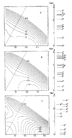
Figure 4: Transition study from a vibrational (A) to a strongly deformed nucleus (C) (from Ref. 22): Left panels: Collective potential energy surfaces and low-energy spectra. Middle panels: Dipole strengths and $\gamma$-absorption cross sections. Right panels: Elastic and Raman $\gamma$-scattering cross sections to low lying collective states.

Subsequently, the DCM was further developed in order to describe a much more general class of potential energy surfaces for the low energy collective d.o.f. allowing a unified description of the GDR for nuclei with quite different collective characteristics by Rezwani et al. [22, 23]. An example, taken from Ref. 22, is shown in Fig. 4 displaying the collective potential energy surface, the absorption strength and cross section and the elastic and inelastic scattering cross sections for three different types of nuclei, resembling a transition from a nucleus with an anharmonic vibrational character (A) to a strongly deformed rotational nucleus (C).

Case A represents a vibrational nucleus with strong anharmonicities, resulting in a shift and splitting of the surface two-phonon triplet. Furthermore, a slight axially symmetric deformation leads to a nonvanishing intrinsic quadrupole moment. Since the nucleus is easily deformable in $\beta$- and $\gamma$-directions, it appears dynamically triaxial resulting in a slight splitting of the dipole strength into three equally spaced states. Moreover, considerable inelastic tensor $\gamma$-scattering into the low-lying $2^{+}$-states is observed.

The opposite situation of a strongly deformed nucleus is displayed by case C. It corresponds to a good axially symmetric rotator with clearly separated ground, $\beta$- and $\gamma$-rotational states. Accordingly the GDR is split into two distinct peaks, and strong Raman-scattering via the tensor polarizability into the $2^{+}$-state of the ground state rotational band appears. The transition between these two extreme cases is represented by case B.

2 Photon scattering off complex nuclei in the $\Delta(1232)$ region

The influence of internal nucleon degrees of freedom constitutes an important field of research in nuclear and medium energy physics. In particular, the role of the lowest excited state of the nucleon, the $\Delta(1232)$ resonance, has been studied in the low energy domain [24] as well as in the energy region of real $\Delta$ excitation in pion production and photo absorption.

For photon scattering in the energy region of about 300 MeV the simplest model is a static approach assuming pure $M1$-scattering off the individual nucleons, whereas the nuclear structure is manifest only via the elastic form factor with respect to the momentum transfer. Then the scattering matrix has the simple form [25]

$$T^{fi}_{\lambda^{\prime}\lambda}=\langle f|\sum_{l=1}^{A}t_{\lambda^{\prime}\lambda}(l)e^{-i(\vec{k}-\vec{k}^{\,\prime})\cdot\vec{r}_{l}}|i\rangle\,,$$ (51)

where the elementary scattering operator is given by

$$t_{\lambda^{\prime}\lambda}(l) = c^{2}\,\Big{(}\frac{\vec{e}_{\lambda^{\prime}}^{\,\prime*}\cdot[\vec{\sigma}_{N\Delta}^{l}\times\vec{k}^{\,\prime}]\,\vec{e}_{\lambda}\cdot[\vec{\sigma}_{\Delta N}^{l}\times\vec{k}\,]}{M_{\Delta}-M_{N}-k_{0}-i\Gamma_{\Delta}/2}$$ (52)

$$+\frac{\vec{e}_{\lambda}\cdot[\vec{\sigma}_{N\Delta}^{l}\times\vec{k}\,]\,\vec{e}_{\lambda^{\prime}}^{\,\prime*}\cdot[\vec{\sigma}_{\Delta N}^{l}\times\vec{k}^{\,\prime}]}{M_{\Delta}-M_{N}+k^{\prime}_{0}-i\Gamma_{\Delta}/2}\,\Big{)}\,.$$

The $N\to\Delta$ spin transition matrix $\vec{\sigma}_{N\Delta}^{l}$ is defined as in Ref. 24. Furthermore,

$$c=G_{M1}^{\Delta N}(M_{\Delta}+M_{N})/(4M_{\Delta}M_{N})\,,$$ (53)

where $M_{N}$, $M_{\Delta}$ and $\Gamma_{\Delta}$ denote respectively nucleon and $\Delta$ mass and width. The latter and the magnetic transition strength $G_{M1}^{\Delta N}$ are fit to the experimental photo absorption cross section of the nucleon in the $\Delta$ resonance region.

In this simple approach nuclear structure enters only via the nuclear form factors of mass and spin (for more details see Ref. 25). A comparison of this approach with experiment for ¹²C and ²⁰⁸Pb is shown in Fig. 5.

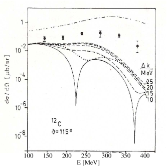
(a) ¹²C

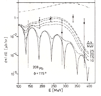
(b) ²⁰⁸Pb

Figure 5: Elastic and quasielastic photon scattering cross sections at $\theta=115^{\circ}$ for ¹²C and ²⁰⁸Pb (from Ref. 25). Experimental data from Ref. 26. Solid curve: elastic scattering in static approach; dashed curves include inelastic contributions up to an excitation energy $\Delta k$; dotted curve: sum rule approach (see Ref. 25 for further details); dash-dotted curve: incoherent sum of elastic elementary $\gamma-N$ scattering cross section.

It turns out, that the resulting calculated cross section largely underestimates the experiment by orders of magnitude for both nuclei. Collective effects in a more refined $\Delta$-hole model for ¹²C by Koch et al. [27] lead to a slight enhancement but the discrepancy remained essentially. However, Hayward and Ziegler [26] already had pointed out that the finite energy resolution with respect to the measured scattered photons of about 10 % would lead to the inclusion of corresponding inelastic contributions in the experimental data.

Subsequently, such inelastic contributions have been studied in Ref. 25 within two simple models: (i) Inelastic scattering into 1-particle-1-hole excitations with excitation energies within an energy interval $\Delta k$ , and (ii) a sum rule approach to the giant resonances as final states (see Ref. 25 for further details). The results of these two models are also shown in Fig. 5. Both approaches show an enhancement due to inelastic contributions, particularly strong for the 1p -1h approach. However, for ¹²C still sizeable strength is missing and a more thorough theoretical treatment is needed.

3 Photon scattering off the deuteron

Now I would like to turn my attention to more fundamental studies with respect to the role of subnuclear degrees of freedom like meson exchange currents (MEC) and and internal nucleon degrees of freedom in terms of nucleon resonances (isobar currents IC) in electromagnetic reactions. Lightest nuclei present ideal laboratories for such studies and I will concentrate on the deuteron for which extensive studies on electromagnetic reactions exist [2, 3, 28, 29].

Figure 6: Diagrammatic representation of pion exchange TPA contributions to the two-photon amplitude.

In photon scattering meson exchange effects do not only appear via MEC in the resonance amplitude but also as additional contributions in the TPA as derived in [30] for a $NN$ one-pion exchange potential (see Fig. 6 for the corresponding diagrams) as well as for isobar contributions.

  

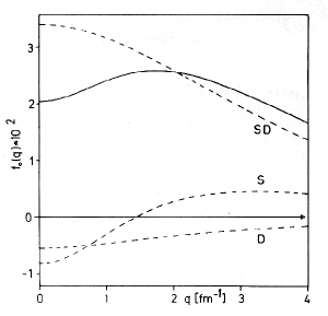
Figure 7: Left panel: Monopole part of $\pi$-exchange transition density for the deuteron (solid curve) from the $\pi$-TPA diagram (d) of Fig. 6. Dashed curves show separate contributions from $S$- and $D$-states and $S-D$ interference. Right panel: Form factor of transition density displayed in the left panel, again with separate contributions (from Ref. 31).

It is intriguing, and indeed had been suggested, that diagram (d) of Fig. 6 allows the extraction of a density form factor of charged mesons in the nucleus (see references in Ref. 31). However, a careful analysis has shown that such an interpretation is not possible [31]. It turns out that the TPA of an exchanged pion (diagram (d) of Fig. 6) reflects the form factor of a pion transition density between the two nucleons and not the virtual pion density inside the deuteron. This feature is illustrated in Fig. 7, where the monopole part of this transition density is displayed. Moreover, as already mentioned above, the diagrams in Fig. 6 are not by itself gauge invariant and thus not separately measurable.

A first realistic calculation of elastic deuteron photon scattering with inclusion of subnuclear effects has been carried out in Ref. 32 taking as reference frame the photon deuteron Breit frame, then $k^{\prime}=k$. Furthermore, small contributions from the c.m. motion have been neglected. For unpolarized photons and deuterons only the scalar polarizability $P^{0}_{ii}(M^{\nu}L,M^{\nu}L,k,k)$ contributes to the elastic scattering cross section. The calculation of the resonance amplitude requires the summation over all excited energies and all possible intermediate states.

As detailed in Ref. 32, a subtracted dispersion relation for the individual polarizabilities of given multipolarity has been assumed using Eq. (41) for the imaginary part of the resonance amplitude (the TPA is real). Thus the real part of the scalar polarizability is determined from

$$Re(P^{RA,0}_{ii}(M^{\nu}L,M^{\nu}L,k,k)) - \delta_{\nu 0}\delta_{L1}\,P^{RA,0}_{ii}(E1,E1,0,0)$$ (54)

$$= (-)^{L+1}\widehat{L}\widehat{I}_{i}\frac{k^{2}}{2\pi^{2}}P\int_{k_{th}}^{\infty}dk^{\prime}\frac{\sigma(M^{\nu}L)(k^{\prime})}{k^{\prime 2}-k^{2}}\,.$$

Here, $k_{th}$ denotes the threshold energy for photo absorption. Since the integral extends in principle up to infinity, one has to include also contributions from particle production above the corresponding threshold energy, e.g. from the total photo pion production cross section for energies above the pion production threshold. These were neglected limiting this approach to the low energy region. For the evaluation of the partial contributions $\sigma(M^{\nu}L)(k)$ to photo disintegration the Reid soft core potential had been used. Besides the one body current and TPA $\pi$-meson exchange currents also $N\Delta$ and $\Delta\Delta$ isobar configurations have been included.

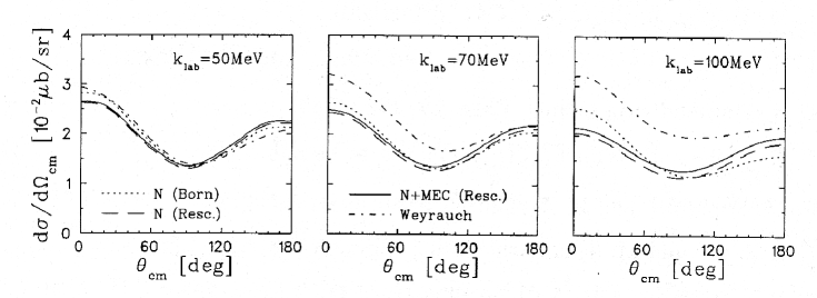
Figure 8: Differential scattering cross sections for photon energies 50, 70 and 100 MeV from Ref. 33. Notation of curves: dotted (labeled “N (Born)”) without FSI and MEC beyond Siegert, dashed (“N (Resc.)”) including FSI but no MEC, and full (“N+MEC (Resc.)”) with FSI and MEC. Dash-dot curves (“Weyrauch”) represent a calculation with a separable interaction from Ref. 35.

A more recent realistic calculation from my group by Wilbois et al. [33] has been based on the solution of the off-shell NN-scattering matrix instead of using dispersion relations. Again inelasticities, which appear above pion production threshold, are excluded, limiting this approach also to low photon energies. For the deuteron bound state and the final state interaction (FSI) the realistic Bonn OBEPQ-B potential has been used. MEC contributions from pion- and rho-meson exchange to the current and the TPA amplitude have been included. For the electric transitions so-called Siegert operators have been used, incorporating thus implicitly the major part of MEC contributions [34]. Fig. 8 displays the resulting differential scattering cross section at three photon energies, 50, 70, and 100 MeV. For comparison the results of another approach by Weyrauch [35] using a separable NN-interaction are also shown. Contributions from internal nucleon structure as manifest, e.g. in nucleon polarizabilities, were neglected in both calculations.

Comparing the dotted with the dashed curves one notes a sizeable increase from FSI with increasing energy, at forward angles a reduction and in the backward region an increase, thus reducing the strong asymmetry of the case without FSI considerably. The additional MEC effects beyond the Siegert operators are quite small for the lowest energy, but become more pronounced at 100 MeV, leading to an overall increase of the cross section. The increasing difference to Weyrauch’s result [35] indicate that the separable interaction used in that work is not appropriate at higher energies.

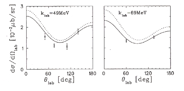
Figure 9: Differential scattering cross sections for photon energies of 49 and 69 MeV (from Ref. 33). Experimental data from Ref 38. Solid curves: complete calculation with nucleon polarizabilities included. Dashed curves: without nucleon polarizabilities.

A comparison with experimental data is shown in Fig. 9. One readily notes a systematic overestimation of the experimental results (dashed curves). An improved description is achieved if the influence of the internal nucleon structure in terms of nucleon polarizabilities is considered (full curves). The additional introduction of the free neutron and proton polarizabilities reduces the cross sections sizeably and gives a better description of the experiment. In view of the fact, that the neutron polarizabilities are not directly measurable, one turns the argument around in order to determine them from photon scattering off the deuteron. However, this procedure is not completely free from model dependencies.

Since then quite a few more theoretical investigations of this reaction using various approaches have been published [36], where the major emphasis had been laid on the extraction of the neutron polarizabilities (for recent results see Ref. 37).

In fact, the deuteron is often used to determine internal neutron properties like polarizabilities and electromagnetic form factors, which otherwise are not available, since free neutron targets are absent. The question of off-shell modification of such internal nucleon properties is thereby left open with the hope that such effects are small since the deuteron is quite a loosly bound system.

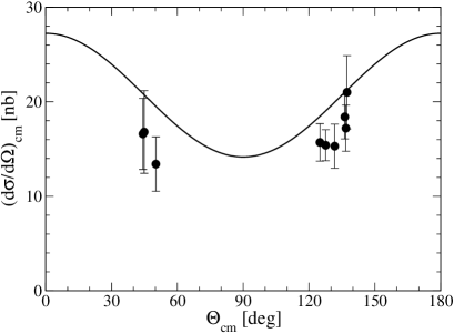
Figure 10: Differential scattering cross section in the unretarded dipole approximation calculated with the Lorentz integral transform method for a photon energy of 55 MeV (from Ref. 40). Experimental data from Ref. 41.

Another interesting aspect which reactions on the deuteron offer is that the deuteron can also serve as a test ground for new theoretical methods. As an illustrative example, I will consider recent work based on the Lorentz integral transform (LIT) method (for a review of this method see Ref. 39). The LIT method is particularly suited for theoretical studies of reactions on complex nuclei. It allows the calculation of reactions without the need of determining the complex final scattering states, reducing this problem to the solution of a bound state equation. Therefore, as a test case for the application of the LIT method to photon scattering reactions, the LIT has been applied to the deuteron for a pure unretarded $E1$ radiation by Bampa et al. [40].

The resulting cross section at one energy is shown in Fig. 10 together with recent experimental data. Nucleon polarizabilities were not included. The slight difference to the more complete calculation at 50 MeV in Fig. 8 is caused by the restriction to $E1$ radiation which is also the reason for the completely symmetric angular distribution around 90^∘ (see Eq. (48)) in contrast to the slight asymmetry at 50 MeV in Fig. 8.

4 Conclusions

With these few examples, I hope to have convinced the reader, that nuclear photon scattering reactions has been and still is a wide and interesting field of research in nuclear structure studies from low energy collective properties to the influence of subnuclear degrees of freedom as manifest e.g. in meson exchange and isobar currents. Hopefully, in the future more experimental results will be available, although the cross sections are quite small compared to hadronic reactions. Of particular interest are scattering experiments on complex nuclei at higher energies in the region of the first nucleon resonance, in order to study the behavior of a nucleon resonance in a nuclear environment.

References

- 1. H. Arenhövel and W. Greiner, Prog. Nucl. Phys. Vol. 10 (Pergamon Press, Oxford 1969), p. 167.
- 2. H. Arenhövel, Workshop on Perspectives in Nuclear Physics at Intermediate Energies, eds. S. Boffi, C. Ciofi degli Atti, and M.M. Giannini (World Scientific, Singapore, 1984), p. 97.
- 3. H. Arenhövel, New Vistas in Electro-Nuclear Physics, eds. E.L. Tomusiak, H.S. Caplan, E.T. Dressler (Plenum Press, New York 1986) p. 251.
- 4. M.-Th. Hütt, A.I. L’vov, A.I. Milstein, and M. Schumacher, Phys. Rep. 323, 457 (2000).
- 5. J.L. Friar, Ann. Phys. (N.Y.) 95, 1428 (1975), and references therein.
- 6. H. Arenhövel and M. Weyrauch, Nucl. Phys. A 457, 573 (1986).
- 7. U. Fano, NBS Technical Note 83 (1960), reprinted in Photonuclear Reactions, eds. E.G. Fuller and E. Hayward (Dowden, Hutchinson & Ross, 1976) p. 338.
- 8. H. Arenhövel, PhD Thesis, University Frankfurt, 1965.
- 9. H. Arenhövel, M. Danos, and W. Greiner, Phys. Rev. 157, 1109 (1967).
- 10. R. Silbar and H. Überall, Nucl. Phys. A 109, 146 (1968).
- 11. R. Silbar, Nucl. Phys. A 118, 389 (1968).
- 12. H. Arenhövel and D. Drechsel, Nucl. Phys. A 233, 153 (1974).
- 13. M.E. Rose, Elementary Theory of Angular Momentum, (Wiley, New York, 1957).
- 14. A.R. Edmonds, Angular Momentum in Quantum Mechanics, (Princeton University Press, Princeton, 1957).
- 15. H. Arenhövel and W. Greiner, Nucl. Phys. 86, 193 (1966).
- 16. M. Danos, Nucl. Phys. 5, 23 (1958); K. Okamoto, Phys. Rev. 110, 143 (1958).
- 17. M. Danos and W. Greiner, Phys. Rev. 134, B284 (1964).
- 18. H.E. Jackson and K.J. Wetzel, Phys. Rev. Lett. 28, 513 (1972).
- 19. T.J. Bowles et al., Phys. Rev. C 24, 1940 (1981).
- 20. H. Arenhövel, Phys. Rev. C 6, 1449 (1972).
- 21. E. Ambler, E.G. Fuller, and H. Marshak, Phys. Rev. 138, B117 (1965).
- 22. V. Rezwani, G. Gneuss, and H. Arenhövel, Phys. Rev. Lett. 25, 1667 (1970).
- 23. V. Rezwani, G. Gneuss, and H. Arenhövel, Nucl. Phys. A 180, 254 (1972).
- 24. H.J. Weber and H. Arenhövel, Phys. Rep. C 36, 277 (1978).
- 25. H. Arenhövel, M. Weyrauch, and P.-G. Reinhard Phys. Lett. B 155, 22 (1985).
- 26. E. Hayward and B. Ziegler, Nucl. Phys. A 414, 333 (1984).
- 27. J.H. Koch, E.J. Moniz, and N. Ohtsuka, Ann. Phys. (N.Y.) 154, 99 (1984).
- 28. H. Arenhövel and M. Sanzone, Few-Body Syst. Suppl. 3, 1 (1991).
- 29. H. Arenhövel, W. Leidemann and E.L. Tomusiak. Eur. Phys. J. A 23, 147 (2005).
- 30. H. Arenhövel, Z. Phys. A 297, 129 (1980).
- 31. M. Weyrauch and H. Arenhövel, Phys. Lett. B 134, 21 (1984).
- 32. M. Weyrauch and H. Arenhövel, Nucl. Phys. A 408, 425 (1983).
- 33. T. Wilbois, P. Wilhelm, and H. Arenhövel, Few-Body Syst. Suppl. 9, 263 (1995).
- 34. H. Arenhövel, Z. Phys. A 302, 25 (1981).
- 35. M. Weyrauch,Phys. Rev. C 41, 880 (1990).
- 36. M.I. Levchuck, Few-Body Syst., Suppl. 9, 439 (1995); J.J. Karakowski and G.A. Miller, Phys. Rev. C 60, 014001 (1999); M.I. Levchuck and A.I. L’vov, Nucl. Phys. A 674, 449 (2000); Nucl. Phys. A 684, 490 (2001); R.P. Hildebrandt, H.W. Grießhammer, T.R. Hemmert, and D.R. Phillips, Nucl.Phys. A 748, 573 (2005); R.P. Hildebrandt, H.W. Grießhammer, and T.R. Hemmert, Eur. Phys. J. A 46, 111 (2010).
- 37. L. S. Myers et al., Phys. Rev. C 92, 025203 (2015).
- 38. M. A. Lucas, Ph.D. thesis, University of Illinois at Urbana-Champaign, unpublished (1994).
- 39. V.D. Efros, W. Leidemann, G. Orlandini, and N. Barnea, J. Phys. G: Nucl. Phys. 34, R459 (2007).
- 40. G. Bampa, W. Leidemann, and H. Arenhövel, Phys. Rev. C 84, 034005 (2011).
- 41. M. Lundin et al., Phys. Rev. Lett. 90, 192501 (2003).