11email: randich@arcetri.astro.it 22institutetext: Department of Physics ‘E.Fermi’, University of Pisa, Largo Bruno Pontecorvo 3, I-56127 Pisa, Italy 33institutetext: INFN, Section of Pisa, Largo Bruno Pontecorvo 3, I-56127 Pisa, Italy 44institutetext: Astrophysics Group, University of Keele, Keele, Staffordshire ST5 5BG, United Kingdom 55institutetext: INAF-Osservatorio Astrofisico di Torino, Via Osservatorio 20, 10025 Pino Torinese, Italy 66institutetext: INAF-Osservatorio Astronomico di Bologna, Via Gobetti 93/3, 40129 Bologna, Italy 77institutetext: Instituto de Astrofìsica de Andalucìa (IAA-CSIC), Glorieta de la Astronomìa, E-18008 Granada, Spain 88institutetext: Laboratoire d’Astrophysique de Bordeaux, Université Bordeaux, CNRS, B18N, Alleée Geoffroy Saint/Hilaire, F-33615 Pessac, France 99institutetext: Dipartimento di Fisica e Astronomia, Università degli Studi di Firenze, Via G. Sansone 1, 50019 Sesto Fiorentino (Firenze), Italy 1010institutetext: Centro de Astrobiología (INTA-CSIC), Departamento de Astrofísica, PO Box 78, E-28691, Villanueva de la Cañada, Madrid, Spain 1111institutetext: Departament de Fìsìca Quantìca i Astrofìsica, Institut Cìencies Cosmos (ICCUB), Universitat de Barcelona, Barcelona, Spain 1212institutetext: Leiden Observatory, Niels Bohrweg 2, 2333 CA Leiden, The Netherlands 1313institutetext: Institute of Theoretical Physics and Astronomy, Vilnius University, Saulėtekio al. 3, LT-10222 Vilnius, Lithuania 1414institutetext: Institute of Astronomy, Madingley Road, University of Cambridge, CB3 0HA, UK 1515institutetext: Lund Observatory, Department of Astronomy and Theoretical Physics, Box 43, SE-221 00 Lund, Sweden 1616institutetext: INAF - Osservatorio Astronomico di Padova, Vicolo dell’Osservatorio 5, 35122 Padova, Italy 1717institutetext: Department of Physics and Astronomy, Uppsala University, Box 516, SE-751 20 Uppsala, Sweden 1818institutetext: Dipartimento di Fisica e Astronomia, Sezione Astrofisica, Università di Catania, via S. Sofia 78, 95123, Catania, Italy 1919institutetext: Nicolaus Copernicus Astronomical Center, Polish Academy of Sciences, ul. Bartycka 18, 00-716, Warsaw, Poland 2020institutetext: Instituto de Física y Astronomiía, Universidad de Valparíso, Chile 2121institutetext: Dipartimento di Fisica e Astronomia, Università di Padova, Vicolo dell’Osservatorio 3, 35122 Padova, Italy 2222institutetext: Núcleo de Astronomá, Universidad Diego Portales, Av. Ejéxrcito 441, Santiago, Chile 2323institutetext: Departamento de Ciencias Fisicas, Universidad Andres Bello, Fernandez Concha 700, Las Condes, Santiago, Chile 2424institutetext: INAF - Osservatorio Astronomico di Palermo, Piazza del Parlamento 1, 90134, Palermo, Italy 2525institutetext: European Southern Observatory, Alonso de Cordova 3107 Vitacura, Santiago de Chile, Chile 2626institutetext: Instituto de Astrofísica e Ciências do Espaço, Universidade do Porto, CAUP, Rua das Estrelas, 4150-762 Porto, Portugal
The Gaia-ESO Survey: open clusters in Gaia-DR1 - a way forward to stellar age calibration ††thanks: Based on observations collected with the FLAMES instrument at VLT/UT2 telescope (Paranal Observatory, ESO, Chile), for the Gaia-ESO Large Public Spectroscopic Survey (188.B-3002, 193.B-0936).
Abstract
Context. Determination and calibration of the ages of stars, which heavily rely on stellar evolutionary models, are very challenging, while representing a crucial aspect in many astrophysical areas.
Aims. We describe the methodologies that, taking advantage of Gaia-DR1 and the Gaia-ESO Survey data, enable the comparison of observed open star cluster sequences with stellar evolutionary models. The final, long-term goal is the exploitation of open clusters as age calibrators.
Methods. We perform a homogeneous analysis of eight open clusters using the Gaia-DR1 TGAS catalogue for bright members and information from the Gaia-ESO Survey for fainter stars. Cluster membership probabilities for the Gaia-ESO Survey targets are derived based on several spectroscopic tracers. The Gaia-ESO Survey also provides the cluster chemical composition. We obtain cluster parallaxes using two methods. The first one relies on the astrometric selection of a sample of bona fide members, while the other one fits the parallax distribution of a larger sample of TGAS sources. Ages and reddening values are recovered through a Bayesian analysis using the 2MASS magnitudes and three sets of standard models. Lithium depletion boundary (LDB) ages are also determined using literature observations and the same models employed for the Bayesian analysis.
Results. For all but one cluster, parallaxes derived by us agree with those presented in Gaia Collaboration et al. (2017), while a discrepancy is found for NGC 2516; we provide evidence supporting our own determination. Our age determinations are robust against models and are generally consistent with literature values.
Conclusions. The systematic parallax errors inherent in the Gaia DR1 data presently limit the precision of our results. Nevertheless, we have been able to place these eight clusters onto the same age scale for the first time, with good agreement between isochronal and LDB ages where there is overlap. Our approach appears promising and demonstrates the potential of combining Gaia and ground-based spectroscopic datasets.
Key Words.:
Parallaxes - Surveys - Stars: evolution - Open Clusters and Associations: general - Open Clusters and Associations: individual: NGC 25161 Introduction
Determination of stellar ages is vital in addressing virtually all branches of stellar and Galactic astrophysics, from the duration of the star formation process and the timescales for the formation and evolution of planetary systems, to the larger-scale formation and evolution of the Milky Way galaxy, and to the age of the Universe. The age of a star cannot be measured directly and it is widely acknowledged that age estimation is one of the most challenging problems in astrophysics (e.g. Palla et al. 2005; Soderblom 2010; Soderblom et al. 2014 and references therein). The most commonly employed method for inferring the ages of stars is the comparison of different quantities which can be derived from observations (colours, temperature, surface gravity, luminosity) with outputs from stellar evolutionary codes, possibly using some appropriate (statistical) inference scheme. This approach is widely used for field stars as well as for star clusters; however, the precision of those ages and, even more importantly, the absolute ages, are set by the fidelity of the evolutionary models, the physical uncertainties inherent to them, and uncertainties in the transformations between theoretical and observational quantities.
Indeed, in spite of considerable progress in understanding stellar physics and evolution in the last decades, several issues are not completely settled, among which we mention the lack of a precise treatment of convection and overshooting; (e.g. Salaris & Cassisi 2015; Viallet et al. 2015); the input physics adopted in the calculations (e.g. opacities, equation of state -EOS-, nuclear reactions etc. –Naylor 2009; Valle et al. 2013; Tognelli et al. 2015b); the effects of internal rotation and magnetic fields (e.g. Eggenberger et al. 2010; Feiden & Chaboyer 2012; Charbonnel et al. 2013; Feiden et al. 2014, 2015); and the outer boundary conditions and atmosphere adopted for the star (e.g. Baraffe et al. 2002). The latter issue is especially true at low masses where the formation of molecules or even dust is a difficult problem and there may be further issues associated with the usual assumption of homogeneous, plane-parallel atmospheres when many stars, particularly those with high levels of magnetic activity, have demonstrable surface inhomogeneities (Jackson & Jeffries 2014; Somers & Pinsonneault 2015; Jeffries et al. 2017). Comparison between theory and observations clearly constitutes a benchmark for stellar evolutionary theory.
Asteroseismology represents a relatively new, very powerful tool for determining stellar ages, in particular for evolved giants (see Miglio et al. 2017 and references therein). However, star clusters remain key age calibrators for stars in all evolutionary phases, and continue to serve as a critical tool to put constraints on evolutionary models. The distribution of non-binary members of a cluster in the colour-magnitude or Hertzsprung-Russell diagrams (CMDs, HRDs) is expected to be very narrow, reflecting the homogeneity in age and chemical composition. At the same time, members of a given cluster cover different masses and evolutionary stages, at the cluster age and metallicity. Each cluster thus represents a snapshot of stellar evolution; linking together observations of many clusters at different ages and chemical compositions empirically reveals the story of stellar evolution, to be compared with the predictions of theoretical models. Much of stellar, and ultimately Galactic, astrophysics hinges on these crucial comparisons between cluster observations and the predictions of the models. Only once the models are appropriately adjusted to represent the data as obtained for a wide range of clusters of different ages and compositions, reliable stellar masses and ages can be determined. Focusing on open clusters (OCs), we note that they play a key role as stellar age calibrators also because the ages of their stars can be estimated using a variety of independent techniques that work accurately (or at least more precisely) when applied to ensembles of stars. These different techniques have different sensitivities to uncertainties in model physics, and in some cases are weakly sensitive to these uncertainties, allowing (almost) model-independent absolute age calibration (e.g. the lithium depletion boundary technique, Burke et al. 2004; Tognelli et al. 2015b).
Precise distances to the clusters are clearly the key to making a big step forward and the Gaia mission (Gaia Collaboration et al. 2016a) will enable a revolution in this area. In the last decade or so a variety of surveys allowed significant progress in deriving empirical CMDs for clusters; however, Gaia will provide precise parallaxes and photometric measurements for several tens or hundreds of nearby OCs and for large samples of members, finally making fully accessible the unique potential of OCs to empirically resolve the CMDs and HRDs and to put tighter constraints on stellar evolutionary models for Population I stars, from the pre-main sequence (PMS) phase to the latest evolutionary stages. In order to best exploit the exquisite information from Gaia, spectroscopy from the ground is also necessary, mainly to firmly derive the cluster chemical composition and to confirm cluster membership using radial velocities and other membership tracers. Ground-based spectroscopy also allows the determination of rotation, effective temperature, surface gravity, and, in general, a full characterisation of the stellar properties down to faint stars.111Radial velocities and astrophysical parameters will also be available from Gaia; however, they are expected to be of lower precision and/or limited to brighter magnitudes than achievable from ground-based spectroscopy.
The Gaia-ESO Large Public Spectroscopic Survey (GES –Gilmore et al. 2012; Randich et al. 2013) is a high-precision, high-resolution survey specifically designed to cover the Gaia range of stellar populations. GES is using the multi-object system FLAMES at ESO VLT (Pasquini et al. 2002), with its high-resolution UVES and its medium-resolution GIRAFFE spectrographs, to target about 105 stars, systematically covering all the major components of the Milky Way, and providing a homogeneous overview of the distributions of kinematics and elemental abundances in stars as faint as and , for GIRAFFE and UVES targets, respectively. GES complements Gaia and vice-versa: in particular, the GES OC dataset, combined with Gaia astrometry (and eventually, spectrophotometry), represents an unrivalled resource to attack the problem of stellar model and age calibration. GES is providing homogeneous and precise measurements of radial velocities, astrophysical parameters, metallicity, detailed abundances for several chemical elements, and assessments of magnetic/accretion activity from H emission for thousands of stars, over a wide range in masses, in about 60–70 OC with ages from a few Myr to several Gyr. As mentioned, in the last decade or so, significant progress has been made both on testing evolutionary models and on star cluster age determination (e.g. Lyra et al. 2006; Silaj & Landstreet 2014; Kopytova et al. 2016). The combination of Gaia and GES cluster datasets will offer clean CMDs and HRDs of well-defined samples of cluster members, allowing further tests of evolutionary models and stellar atmospheres, and making it possible to choose the best models to estimate ages.
The first intermediate Gaia data release (Gaia-DR1 -Gaia Collaboration et al. 2016b) includes positions and Gaia G band magnitudes for about 1 billion stars, as well as the five-parameter astrometric solution - positions, parallaxes, and proper motions - for about two million sources in common between the Tycho-2 Catalogue (Høg et al. 2000) and Gaia. This part of the Gaia DR1 dataset is based on the Tycho-Gaia Astrometric Solution (TGAS -Michalik et al. 2015; Lindegren et al. 2016), obtained by combining the Tycho 2 and Gaia data together, which provides a long enough baseline to break the degeneracy between motion and parallax. The limiting magnitude of the TGAS catalogue is mag; bright stars in several nearby cluster fields are thus contained in it, allowing not only the validation of Gaia astrometry, but also the determination of average cluster parallaxes (Gaia Collaboration et al. 2017 -hereafter VL17). A fraction of the clusters whose members are included in TGAS have been observed by GES during the first 30 months of data taking and the parameters of the target stars have been derived during the latest analysis cycle (iDR4) and released internally to the consortium in the GEiDR4Final catalogue.222The GEiDR4Final catalogue is available for the members of the GES consortium at http:/ges.roe.ac.uk/. Parameters for a large fraction of the stars have also been released to ESO during the Phase 3 delivery and are publicly available at the ESO archive facility (http://www.eso.org/qi). Within each cluster, the GES target samples are at this stage generally complementary to the TGAS ones, mostly including stars much fainter than the TGAS limit, although a few stars in common are present in some of the clusters. The two datasets, the TGAS one for the bright members and the GES one for the fainter stars down to the 19 magnitude in the band, will hence be used mainly independently. Namely, the GES data will allow us to define the cluster sequences in a way that is unbiased with respect to the CMD, over a broad magnitude range (equivalent to a range of masses). GES data will also yield the cluster chemical composition. Members identified in TGAS will instead mainly be employed to determine the cluster parallaxes. The two datasets together will critically allow us to match evolutionary models, with metallicity and distance as fixed parameters, and to put the clusters into a model-dependent age sequence.
Gaia-DR2 will yield more precise and accurate parallaxes for stars down to about the 20th magnitude, allowing one to reach more distant clusters and/or lower mass members in nearby clusters. At the same time, GES will complete observations and analysis of all its sample clusters. Along with the GES data, Gaia-DR2 will thus make possible a more detailed analysis based on both a larger number of clusters covering a larger interval of ages and metallicity, and on more secure astrometry. With the present analysis and paper, however, we aim to set the methodology, to identify major sources of uncertainty, and to show, exploiting Gaia-DR1 already, how the combination of Gaia and GES cluster data can be used to calibrate stellar evolution and ages. The methods that we outline here will then be exploited using Gaia-DR2 and the full sample of GES OCs.
The paper is structured as follows: in Sect. 2 we present the sample OCs, GES target selection, available spectroscopic information, and cluster chemical composition. The cluster membership determination using GES data is presented in Sect. 3, while the astrometric analysis and determination of the cluster parallaxes are discussed in Sect. 4. Section 5 is dedicated to the comparison with different evolutionary models and age determination; the presentation and discussion of the results, and conclusions are summarised in Sects. 6 and 7, respectively.
2 The sample clusters and Gaia-ESO Survey information
We considered clusters that have bright stars included in TGAS, have been observed by GES, and have been analysed in iDR4. We further selected OCs close enough that their parallaxes are not greatly affected by Gaia-DR1 systematic errors in parallax (see Sect. 4), and old enough not to be characterised by possible age dispersions. The final sample includes eight clusters, listed in Table 1, along with their main properties from the literature.
| Cluster | RA | DEC | age | ref. | E() | ref. | pre-Gaia | ref. |
|---|---|---|---|---|---|---|---|---|
| J2000 | (Myr) | distance modulus | ||||||
| NGC 2451A | 07 44 27.00 | 40 00.00 | 50-80 | (1), (2) | 0.01 | (2) | van Leeuwen (2009) | |
| NGC 2451B | 07 44 27.00 | 40 00.00 | 50 | (1) | 0.05-0.12 | (3), (4) | Carrier et al. (1999) | |
| NGC 2516 | 07 58 04.00 | 45 12.00 | 70-150 | (5), (6), (7), (8) | 0.09-0.15 | (9), (10), (11) | 7.68 | van Leeuwen (2009) |
| NGC 2547 | 08 10 25.70 | 10 03.00 | 35-45 | (12), (13), (14) | 0.038-0.12 | (9), (13), (15) | 8.38 | van Leeuwen (2009) |
| IC 2391 | 08 40 32.00 | 02 00.00 | 30-50 | (16), (17), (18) | (9) | 5.80 | van Leeuwen (2009) | |
| IC 2602 | 10 42 58.00 | 24 00.00 | 30-46 | (18), (19) | 0.02-0.04 | (9), (20) | 5.86 | van Leeuwen (2009) |
| IC 4665 | 17 46 18.00 | 43 00.00 | 28-40 | (21), (22) | 0.16-0.19 | (9), (22) | 7.75 | van Leeuwen (2009) |
| NGC 6633 | 18 27 15.00 | 30 30.00 | 425-575 | (24), (25), (26) | 0.17-0.18 | (9), (23) | 7.87 | van Leeuwen (2009) |
(1) Hünsch et al. (2003); (2) Platais et al. (2001); (3) Carrier et al. (1999); (4) Balog et al. (2009); (5) Jeffries et al. (1998); (6) Lyra et al. (2006); (7) Silaj & Landstreet (2014); (8) Tadross et al. (2002); (9) Nicolet (1981), (10) Sung et al. (2002); (11) Terndrup et al. (2002); (12) Jeffries & Oliveira (2005); (13) Naylor & Jeffries (2006); (14) Paunzen et al. (2014); (15) Claria (1982); (16) Barrado y Navascués (1999); (17) Barrado y Navascués (2004); (18) Stauffer et al. (1997); (19) Dobbie et al. (2010); (20) Hill & Perry (1969); (21) Manzi et al. (2008) ; (22) Cargile & James (2010); (23) Gurklyte & Strayzis (1981); (24) van Leeuwen (2009); (25) Dias et al. (2002); (26) Williams & Bolte (2007).
2.1 Target selection and characteristics
The selection of the target stars within each cluster is described in detail in Bragaglia et al. (in preparation). We summarise here the relevant features. Briefly, the selection was performed following two main criteria: a) obtaining a large and unbiased sample of cluster candidates to be observed with the GIRAFFE fibres; and b) obtaining a smaller sample of brighter stars to be observed with the UVES fibres. More specifically, GIRAFFE targets were selected using 2MASS near-IR photometry (Skrutskie et al., 2006), along with many public sources of optical photometry. The cluster sequences were identified in optical and near-IR CMDs, with the help of known members from the literature and/or isochrones. We then inclusively selected candidates, considering stars covering the same spatial extension as known members and lying in a generous band around the identified cluster sequences. When information was available, UVES targets were instead chosen among the most likely previously known cluster members. By observing stars in all evolutionary phases and by combining the two approaches, we aim to derive a comprehensive picture of each cluster and of the complete sample of clusters. The number of candidates observed in the field of each cluster varies from about 100-200 to almost 2000, but significant contamination is expected (even among the UVES targets) due to our inclusive selection of candidates. Most of the OCs in the present paper are relatively young (age Myr, but older than Myr) and the targets (both UVES and GIRAFFE ones) are stars on the [pre/zero-age] main sequence. The only cluster which is slightly older is NGC 6633 (age about 600 Myr), where we observed stars on the main sequence and in the red clump phase.
We refer to Pancino et al. (2017) for complete information on the GIRAFFE gratings employed in GES. We just mention here that the targets in the eight sample clusters are generally of late spectral type (F to M), with only a few earlier-type stars. We mainly observed them with the GIRAFFE setup HR15N, where H and the Li i 6708Å line are located. About 5-10 % of the targets were observed with UVES and the 520 and 580 setups for stars earlier and later than F-type, respectively.
2.2 Spectrum analysis and products
GES data reduction and spectrum analysis, including homogenisation have been described in a number of papers (Sacco et al. 2014; Smiljanic et al. 2014; Jackson et al. 2015; Lanzafame et al. 2015). In summary, pipeline data reduction, as well as radial and rotational velocity determinations are centralised and performed at the Cambridge Astronomy Survey Unit (CASU) for GIRAFFE and at Arcetri for UVES spectra, respectively. Spectrum analysis is instead distributed among five working groups (WGs), depending on the stellar-type and/or instrument and/or setup. From at least two up to several nodes contribute to the analysis within each WG; node astrophysical parameters and abundances are first homogenised within each WG and subsequently homogenised across WGs, to put them on a common scale. Homogenisation is performed using several calibrators, including benchmark stars and calibration open/globular clusters, selected as described in Pancino et al. (2017). Radial velocities from the different instruments and settings are also homogenised. The homogenised values constitute the recommended set and are included in the GEiDR4Final catalogue: unless otherwise mentioned, this paper makes use of these recommended values. The dataset released in the GEiDR4Final catalogue includes radial and projected equatorial rotational velocities (RV and v), stellar parameters (Teff, g, and/or index -see Damiani et al. 2014), global metallicity [Fe/H], and equivalent widths of the Li i 6708Å feature (EWLi); for UVES targets individual abundances for a variety of species, such as light, , Fe–peak, and neutron capture elements are also provided. For each of the eight clusters and all the candidates considered in this study, the Gaia-ESO products are provided in the online tables.
2.3 Metallicity and -element abundances
Overall metallicities for the eight clusters included in this analysis were derived, based on the GEiDR4Final catalogue, by Jacobson et al. (2016 –NGC 2516 and NGC 6633) and by Spina et al. (2017 –the remaining clusters) and are listed in Table 2.
element abundances were available for two of the sample clusters only (NGC 2516 and NGC 6633, also based on GEiDR4Final –Magrini et al. 2017). Thus, we consistently derived them here for the other clusters. Specifically, average [El/Fe] ratios were obtained based on the secure cluster members observed with UVES (see following section) and considering only stars with rotational velocities below 15 km s-1. [El/Fe] values are normalised to the GES recommended abundances for the Sun (see Magrini et al. 2017). The results are listed in Table 2, where for each cluster we present the metallicity and the abundance ratios with their 1- dispersion. In the second to the last column we report the mean [/Fe], computed by averaging the available elements. As discussed already by Spina et al. (2017), all clusters have close to solar metallicities with a relatively small dispersion. On the other hand, the table shows some scatter in elemental abundances, both within clusters and across clusters, with some elements being systematically somewhat below or above solar. Given the uncertainties, however, we can safely conclude (at least for the purposes of the present work) that all the clusters have [/Fe] consistent with the solar ratio, that is, [/Fe]=0 dex. Whilst in the following we will assume [Fe/H] for all of the clusters, the effect of metallicity on the recovered ages and reddening values will be briefly discussed in Sect. 6.
| Cluster | [Fe/H] | [MgI/Fe] | [SiI/Fe] | [CaI/Fe] | [TiI/Fe] | [/Fe] | [/Fe] provenance |
|---|---|---|---|---|---|---|---|
| NGC 2451A | 0.02 | :: | :: | 0.02:: | :: | this paper, 1 star | |
| NGC 2451B | 0.01 | :: | :: | 0.01:: | 0.05:: | this paper, 1 star | |
| NGC 2516 | Magrini et al. (2017) | ||||||
| NGC 2547 | this paper, 2 stars | ||||||
| IC 2391 | this paper 2 stars | ||||||
| IC 2602 | this paper, 7 stars | ||||||
| IC 4665 | this paper, 6 stars | ||||||
| NGC 6633 | Magrini et al. (2017) |
3 Gaia-ESO Survey cluster membership
As described in Sect. 2.1, GES cluster target selection was designed to be inclusive; as a result, many of the observed targets are not cluster members. A key aim of this paper is to compare clean cluster sequences with theoretical predictions in the CM diagrams and so these interlopers need to be removed, but without relying on information from these two diagrams, to avoid biasing the final results. In this Subsection we describe a homogeneous approach to membership selection that was applied to all the clusters.
To perform the membership analysis, which was applied to both GIRAFFE and UVES targets, we used the available photometry, together with information from GES products and summarised at the end of Sect. 2.2. All of these data are available for the majority of stars, but in what follows, we required a star to have a Teff, g or , and a RV in order to be considered as a candidate member. As mentioned, most of the data come from the GEiDR4Final internal release except v, where calibration issues meant that the previous release (iDR2/3) values were used in preference and are thus only available for three of the considered clusters (NGC 2547, IC 4665 and NGC 2516). Also, for a few stars EWLi were not available in the GEiDR4Final catalogue; in those cases, EWLi determined by one of the nodes were used.
RV uncertainties are important to derive the RV distribution and membership probabilities. For the clusters with available v data (see above) RV uncertainties were calculated according to the detailed prescription described by Jackson et al. (2015), which takes into account stellar rotation. For the remaining clusters, the uncertainties were instead adopted from the GEiDR4Final catalogue. The comparison of the calculated uncertainties with those from the GEiDR4Final catalogue for candidate members of NGC 2547, IC 4665 and NGC 2516 showed that using the GEiDR4Final catalogue RV uncertainty (where necessary) has only a marginal effect on the average membership probability as a function of RV. At worst, the effect of using the GEiDR4Final catalogue RV uncertainty is to change the membership classifications of a few targets in each cluster where the measured RV is close to the boundary of plausible cluster members.
3.1 The selection sequence
Whilst we initially retained all targets observed with the UVES 520 setup and available parameters, the samples of stars observed with HR15N and UVES 580 were cleaned of almost certain non-members in the following way.
-
1.
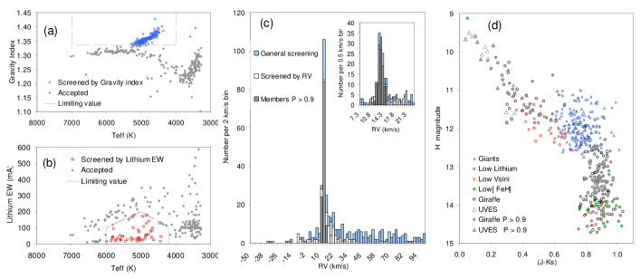
For all clusters, likely giant contaminants were removed using a modified version of the index (, where is the temperature-sensitive index – see Damiani et al. 2014), which removes the temperature sensitivity of the index. Targets with K and were thus rejected as giants. By comparing with for the subset of stars for which the gravity is also available, we find that this threshold corresponds to . We note that for NGC 6633 UVES sample giants were not discarded.
-
2.
The presence of lithium in the photosphere is an excellent empirical age indicator for low-mass stars within given Teff ranges (e.g. Soderblom et al. 2014). By examining compiled data from the literature for the sample clusters and other clusters in the same age interval (e.g. Soderblom et al. 1993; Jeffries et al. 1998; Randich et al. 2001; Sestito & Randich 2005; Jeffries et al. 2014), we designed simple filters in the EWLi versus Teff plane. These filters allowed the inclusion of almost all previously known members of the clusters at their assumed ages, whilst excluding a significant fraction of older contaminant stars at the same Teff. More specifically, if a valid EWLi measurement (or upper limit) was present for a star in the Teff range indicated in Table 3, but was below the Teff-dependent threshold, then the star was rejected. The separation between field stars and cluster members becomes smaller at older ages and Li selection was not applied for NGC 6633.
-
3.
Targets with were excluded, since all of the clusters have approximately a solar metallicity (see Sect. 2.2). A very conservative threshold was adopted here.
-
4.
For targets with valid v estimates, if v km s-1 (unresolved broadening at the GES spectral resolution) the target was rejected as unlikely to be a cluster member. This threshold was only applied to those stars outside the Teff range for which the lithium test was valid. The rationale here is that such stars are either relatively hot, in which case they do not spin down with age in the same way as cooler stars; or, they are so cool that their spin down timescales are extremely long, such that no slow rotators are expected at the ages of the clusters considered here. Of course the unknown inclination angle might mean that a small fraction of rapidly rotating stars have a small v, but we were prepared to accept this loss in favour of a more efficient rejection of non-members.
The first of the above steps (gravity) identified the majority of contaminants. Lithium selection was very effective in the youngest clusters, becoming less so in older clusters, yet still rejecting % of the remaining candidates. Very few candidates were removed because of their low metallicity or slow rotation.
3.2 Radial velocity distributions and membership probabilities
The radial velocity distributions of the filtered candidate members for each cluster were modelled using the maximum likelihood technique described in Jeffries et al. (2014), originally proposed by Pryor & Meylan (1993) and updated by Cottar et al. (2012) to include the contribution of binaries. This technique assumes that the observed radial velocities are taken from an intrinsic model broadened by the observational RV uncertainties and the effects of unresolved binaries; the latter have a distribution of RV offsets expected from a set of randomly oriented SB1 binary systems with a specified distribution of orbital periods, eccentricities, and mass ratios. The total likelihood of a star’s observed RV is then given by the sum of its likelihood if it were a single star and its likelihood if it were in an unresolved binary.
| (1) |
where and are the likelihood of single and binary stars and is the adopted binary fraction. Given a model specified by a number of free parameters (see below), the best-fitting model is found by calculating the likelihood for each star and then maximising the summed logarithmic likelihood for all stars by varying the model parameters over a grid of possibilities.
For the clusters considered here we constructed models that consisted of multiple Gaussian components. One broad Gaussian was used to represent the background of contaminating stars that are still likely to be in the sample after filtering. The clusters themselves were modelled as single Gaussians, except for NGC 2547 and NGC 2451, where two Gaussians were required to adequately model the RV distribution. In the former case, the second kinematic population was originally discovered by Sacco et al. (2015) and will not be considered further in the present paper. In the case of NGC 2451 the two populations correspond to clusters A and B, which will be considered separately. The characteristics of the binary population were fixed in each case to be those of the solar-type field stars estimated by Raghavan et al. (2010), with a binary fraction of 0.46. The exact details of the assumed binary parameters make little difference to the membership probabilities and ultimate selection of candidates to compare with isochrones.
Once the best-fitting parameters of the intrinsic distributions were found, the probability of individual stars belonging to the cluster component(s) was calculated, assuming that each star must be a member of either the cluster component(s) or the background. We caution that these samples will not be cleaned of all contamination. For example, a star with still has a 10% chance of being an unrelated contaminating star. For the comparison with theoretical models we conservatively retained all the objects with , except for NGC 2415A and NGC 6633 where we considered , as there are no stars with , due to the less well defined RV peak and broader distribution.
| Cluster | T1 | T2 | T3 | EWLi1 | EWLi2 | EWLi3 |
|---|---|---|---|---|---|---|
| (K) | (mÅ) | |||||
| All but NGC 2516 | 4200 | 5000 | 6000 | 100 | 200 | 100 |
| NGC 2516 | 4600 | 5000 | 6000 | 50 | 100 | 50 |
| NGC 6633 | 4600 | 5000 | 6000 | 0 | 0 | 0 |
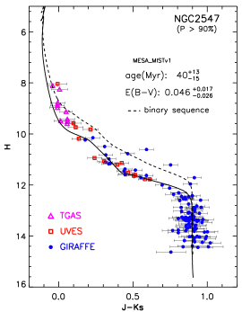
As an example, the selection sequence and the results for the cluster NGC 2547 are summarised in Fig. 1.
4 TGAS analysis: Cluster membership and parallaxes
TGAS-based parallaxes for all clusters included in this paper except NGC 2451B have been published in VL17. Nevertheless, we re-derived them here to independently test our methodologies and because we aim to perform a uniform analysis which would also include NGC 2451B.
Our approach is based on the trigonometric parallaxes and proper motions of the bright stars included in the TGAS catalogue. We first compiled samples of previously known cluster candidates brighter than mag for each cluster, using catalogues available in the literature. These lists are used as initial guesses for the TGAS membership analysis; hence, we adopted a conservative approach and considered only high-probability members from the literature. Also, these samples do not include GES targets, which, as noted, are typically fainter than the TGAS limit. We then cross-matched these samples of likely cluster members with the TGAS catalogue, finding at least ten members for each cluster with available astrometric parameters.
As mentioned, the samples of literature members were used to compute the initial estimates of the astrometric parameters (i.e. the basic statistics of the proper motions and parallaxes) needed to refine the selection of the candidate cluster members from the whole TGAS catalogue. After that, we applied two complementary methods to analyse the TGAS subsets and to estimate the cluster trigonometric parallaxes. The first procedure relies on a conservative selection of a sample of bona fide astrometric members, based on tight confidence levels that minimise the contamination of the false positives. Conversely, the second procedure adopts larger thresholds and fits the parallax distribution of a larger sample of TGAS sources with a model representing both cluster and field stars. In the following, we describe in detail these two procedures and compare the results in Table 4.
4.1 Analysis of the ‘bona fide’ cluster members
We selected TGAS sources centred on the nominal cluster position listed in Table 1 and within a search radius between and ; the radii correspond to 4-6 pc at the expected distances of the clusters. The smaller values were usually adopted for the clusters with proper motions that were not well separated from the field stars. Also, since the search radii are of the order or smaller than the scale-length, , of the astrometric systematic error in TGAS (Lindegren et al. 2016), we can reasonably assume that a global zero point uncertainty will possibly affect our parallax and distance estimations.
After identifying all TGAS sources within the search area, we checked their astrometric solution and rejected stars with formal errors on parallaxes and proper motions larger than 0.6 mas and 3 mas yr-1, respectively. The adopted thresholds were chosen after visual inspection of the corresponding distributions, in order to remove outliers corresponding to anomalous astrometric solutions. In addition, we selected only TGAS astrometric solutions based on a minimum of 50 CCD observations and affected by an excess of noise555This parameter represents the residual error of the single star fitting. See Lindegren et al. (2016) for further details. mas in order to discard astrometric binaries and other anomalous cases.
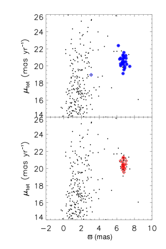
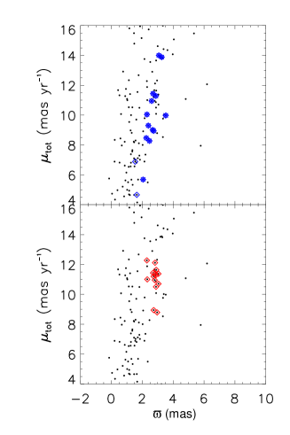
Candidate cluster members were then selected in the 3D space of parallaxes and proper motions, , by means of the following procedure. We first estimated the mean values and dispersions of the cluster members selected from the literature. Secondly, in order to remove false positives, we further rejected catalogue sources by applying a threshold on both proper motions and parallaxes. Then, we recomputed the first- and second-order moments of the three dimensional (3D) distribution, including the correlation between proper motions and parallaxes, and for the final selection we assumed a probability distribution in the form of a 3D Gaussian ellipsoid:
| (2) |
where is the function defined by:
| (3) |
Here, represents the determinant of the symmetrical matrix of the empirical correlation coefficients (for ), and denotes the cofactor of the corresponding correlation element in (Trumpler & Weaver 1953). A 2 threshold, with , corresponding to a confidence level (C.L.) of 73.8% in 3D, was usually applied to select the bona fide cluster members, although a more conservative threshold of 1.5 (C.L. 48%) was adopted for some clusters (see Table 4), to further minimise the contamination of field stars 666 The function in Eq. 2 represents a 3D Gaussian distribution, where is the sum of the squared and normalised residuals. .
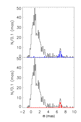
The results of IC 2602 and NGC 2451 B are shown as examples in Figs. 3 and 3. For IC 2602, the mean proper motions are well separated from the field stars, while for NGC 2451B, the mean proper motions overlap with the field. We also notice that, particularly for NGC 2451B, the candidate members collected from the literature (blue symbols) appear contaminated by several false members, in spite of our initial conservative selection; nevertheless, the left panels of Figs. 3-3 clearly show that the resulting astrometrically selected members (red symbols) match properly the cluster peak in the parallax distribution of the complete set of TGAS sources.
Finally, the cluster parallax was derived as a weighted mean of the parallaxes of the selected members: . The corresponding error was estimated using the standard formula, , which does not depend on the residuals and thus is not biased due to the cuts applied to the tail of the distribution by the procedure described above. We point out that the formal error on the weighted mean, , does not include the uncertainty due to the possible systematic errors affecting the TGAS catalogue. The latter was considered when converting parallaxes to distances.
The results are reported in Table 4 and compared to the independent results provided by the method based on the Gaussian maximum likelihood fitting that is described in more detail in the following section.
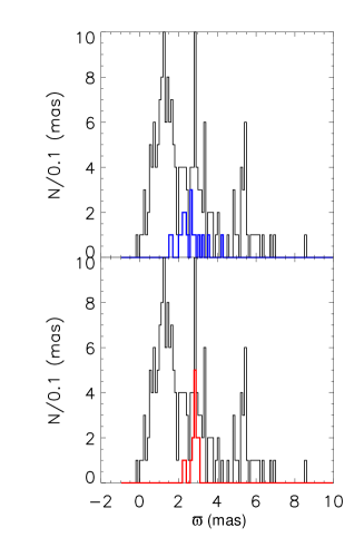
4.2 Analysis of the loosely selected members
In a different approach, for reference purposes, we pre-selected all TGAS stars in the clusters of interest with positions, proper motions, and parallaxes loosely compatible with those of the selected literature cluster members described above. The selection was performed as follows:
where is a generous radius for membership selection (1 deg), and are the centre coordinates, and are the median proper motions of the literature members with their dispersions, and , while is the median parallax with its dispersion, . The selection in parallax was less restrictive than that on proper motions in order to have a large enough range of parallaxes to characterise the distribution of field stars.
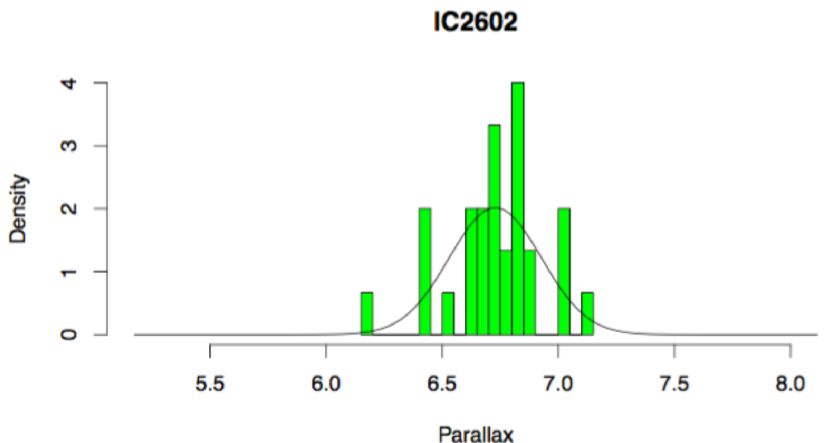
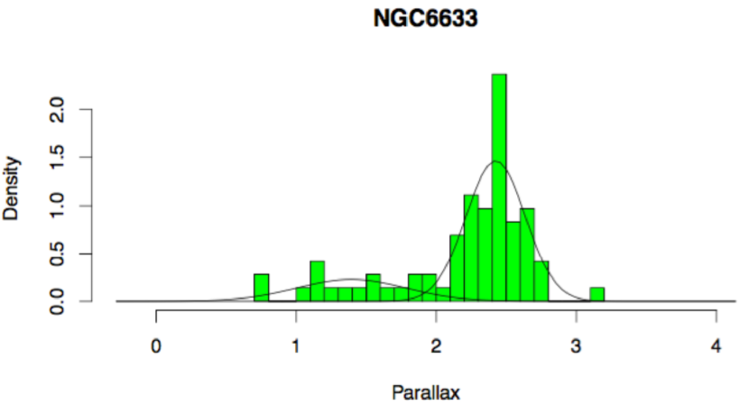
We then fitted the distribution of parallaxes of the selected stars with both one Gaussian and the sum of two Gaussians with different mean and sigma, and maximum likelihood estimation (MLE). Specifically, we employed the likelihood estimator defined by Pryor & Meylan (1993), Walker et al. (2006), and Martin et al. (2007), which takes into account the errors on measurements as well. Namely, the estimated uncertainty in the measurements was included in the model separately from the intrinsic dispersion of the cluster and background. We mention in passing that this approach is very similar to the one adopted in Sect. 3 for the GES RV analysis, except that it does not take into account the presence of binaries.
In cases with a negligible field contamination (IC 2602 being the best case, Fig. 5), the one or two Gaussians fits gave the same result for the cluster parallax, within the uncertainties. In more difficult cases (NGC 2451 B being the worst case), we observed distortions in the shape of the distribution, or multiple peaks and the fits with the one or two Gaussians yielded different values of the cluster parallaxes; in these cases we adopted the two-Gaussians solution.
We note that in the case of NGC 2451 B, the high field contamination forced us to restrict the cluster radius to instead of , and the cut in proper motion to 2.2 rather than 3 . We also mention that the Gaussian distribution was not always the best model for the residual field population after the loose pre-selection, but it granted an accurate positioning of the cluster Gaussian by removing field stars in a satisfactory way after visual inspection (see the case of NGC 6633 in Fig. 5).
The results are listed in Table 4, where the number of fitted Gaussians is also reported. The formal errors on the parallax () were computed with the formulas by Pryor & Meylan (1993), which take the TGAS parallax errors into account. The observed dispersions in the parallax distributions, in Table 4, are significantly larger than the cluster’s depth in parallax space (the latter being at most of the order of 10 as for the closest clusters). As a result, the fitted intrinsic cluster dispersions with the adopted MLE formulation were negligible (close to zero), meaning that most of the observed spread was attributed to measurement errors.
4.3 Reference distances and comparison with other determinations
Table 4 displays results that indicate an extremely good agreement between the two complementary procedures, supporting the internal consistency of our results. In particular, this means that false positives contaminating the selected cluster members do not significantly alter the mean parallax.
The table also lists the parallaxes reported in the literature before Gaia (mainly derived from Hipparcos data) and those derived by VL17. Considering pre-Gaia determinations, the table shows that for five of the clusters our parallaxes agree well with previous determinations, while the agreement is less good for NGC 2516, NGC 2547, and NGC 6633. For the latter cluster the parallaxes are only marginally inconsistent, given the large error of the Hipparcos value, while in the case of NGC 2516 the discrepancy is in principle similar to the expected systematic ( mas) discussed by Lindegren et al. (2016). The disagreement for NGC 2547 is much larger; interestingly, in this case the distance modulus derived from our parallax (see Table 6) is consistent with that () derived by Naylor & Jeffries (2006), by fitting the CMDs with isochrones.
The comparison with VL17 indicates an excellent agreement for most clusters. In particular, VL17 parallaxes for NGC 6633 and NGC 2547 are much closer to our own estimates than to those from Hipparcos. However, a discrepancy between our results and VL17 is present for NGC 2451A and, again, NGC 2516. Whilst the difference for NGC 2451A (10 pc in distance) is not statistically significant, the discrepancy for NGC 2516 is greater than and equivalent to pc in distance.
In order to double check our parallax determination for NGC 2516, we ran again the procedure described in Sect. 4.1, but adopting different initial conditions. Namely, we did not start the analysis from a list of known literature members, but we considered the initial values from van Leeuwen (2009 –VL09), as done by VL17. The 53 TGAS cluster members selected in this way within a radius of show a mean proper motion and a mean parallax . The results are hence in good agreement with the astrometric parameters reported in Table 4, confirming the consistency of our procedure. We also note that this sample includes eight bright Hipparcos sources, whose astrometric parameters are expected to be more accurate than those of the Tycho 2 sources in TGAS. In particular, the correlation between the parallax and proper motions are usually much smaller for the Hipparcos stars. As shown in Table 5, all these stars have parallaxes in the range mas, comparable to the mean parallax of the whole sample, although slightly smaller (possibly due to colour and magnitude systematics). We hence conclude that our determination of the parallax of NGC 2516 seems not only to be solid against initial assumptions, but also validated by the presence of the Hipparcos stars. In Sect. 6.3 we will discuss the age and reddening estimates using VL17 parallax for this cluster.
Table 6 summarises the astrometric parameters of all the sample clusters resulting from the first procedure. We adopt these parameters as reference values in the following sections.
| bona fide cluster members | Loosely selected members | VL09 | VL17 | |||||||||||
| Cluster | C.L. | N | N | nGauss | ||||||||||
| (deg) | (mas) | (mas) | (mas) | (mas) | (mas) | (mas) | (mas) | (mas) | (mas) | |||||
| NGC 2451A | 2.0 | 25 | 5.266 | 0.061 | 0.504 | 1 | 5.59 | 0.11 | ||||||
| NGC 2451B | 1.5 | 46 | 2.763 | 0.041 | 0.354 | 2 | – | – | ||||||
| NGC 2516 | 1.5 | 33 | 2.588 | 0.052 | 0.467 | 1 | 2.99 | 0.08 | ||||||
| NGC 2547 | 1.5 | 17 | 2.720 | 0.071 | 0.224 | 1 | 2.79 | 0.06 | ||||||
| IC 2391 | 2.0 | 24 | 6.829 | 0.055 | 0.216 | 2 | 7.01 | 0.11 | ||||||
| IC 2602 | 1.5 | 2.0 | 30 | 6.749 | 0.051 | 0.198 | 1 | 6.74 | 0.05 | |||||
| IC 4665 | 2.0 | 15 | 2.784 | 0.073 | 0.124 | 2 | 2.83 | 0.05 | ||||||
| NGC 6633 | 1.5 | 72 | 2.438 | 0.032 | 0.212 | 2 | 2.37 | 0.03 | ||||||
| HIP ID | |||
|---|---|---|---|
| mag | mas | mas | |
| 38759 | 8.874 | 2.37 | 0.22 |
| 38739 | 8.163 | 2.41 | 0.24 |
| 38906 | 6.859 | 2.44 | 0.24 |
| 38966 | 7.138 | 2.20 | 0.24 |
| 39438 | 8.300 | 2.50 | 0.24 |
| 39562 | 7.683 | 2.62 | 0.23 |
| 120401 | 9.170 | 2.27 | 0.28 |
| 120404 | 7.615 | 2.28 | 0.24 |
| Cluster | |||||
|---|---|---|---|---|---|
| (mas) | (pc) | (mag) | |||
| NGC 2451A | |||||
| NGC 2451B | |||||
| NGC 2516 | |||||
| NGC 2547 | |||||
| IC 2391 | |||||
| IC 2602 | |||||
| IC 4665 | |||||
| NGC 6633 |
5 Comparison between theory and observations
As mentioned in the introduction, the comparison between HRDs/CMDs and theoretical isochrones represents a key tool for testing models of stellar evolution and to derive the cluster ages. Two of the main uncertainties affecting the comparison of this procedure are the cluster distance and chemical composition; in the present case, GES analysis provides the metallicity and abundance ratios, while the TGAS parallax measurements provide a direct cluster distance determination, enabling already a step forward. In the near future we expect that the Gaia parallaxes will be of much higher precision and uncertainties in the distance will become much less important, allowing even more detailed comparisons with the models. Nevertheless, as we will show in the following sections, the TGAS data already allow us to test the methodology, to identify main sources of errors, and to achieve new results.
5.1 The evolutionary models
In this paper we make use of and compare the results of some recent, updated, and widely used grids of evolutionary models. Namely, we chose the MIST database (the MESA isochrone set, see Paxton et al., 2011, 2013, 2015) in the Choi et al. (2016) and Dotter (2016) version999available at the link http://waps.cfa.harvard.edu/MIST/, the PARSEC (1.2S version, see Chen et al., 2014; Bressan et al., 2012)101010available at the link http://stev.oapd.inaf.it/cgi-bin/cmd, and the PROSECCO models. We note that we only considered models that cover the whole observed mass range of the sample clusters and include standard physics only. Also, the PROSECCO evolutionary tracks were calculated specifically for this work by means of the Pisa version of the FRANEC evolutionary code (Tognelli et al., 2011; Dell’Omodarme et al., 2012; Tognelli et al., 2015a, b). For the comparison we adopted stellar models with [Fe/H]= and [/Fe]=0, compatibly with the results given in Table 2. All the grids of evolutionary models adopt updated input physics and estimates of the solar abundance mixture, summarised in Table 7. We refer to the cited papers for a detailed description.
The precise analysis of the effects of the different choices in the input physics is beyond the scope of the present work. Hence, we only briefly present in Appendix. A a comparison of the predictions of the selected sets of models to highlight the main differences among them, referring the interested reader to previous detailed studies on this topic (i.e. Chabrier & Baraffe, 1997; Siess, 2001; Montalbán et al., 2004; Tognelli et al., 2011).
| Code: | EOS | Radiative Opacity | Boundary Conditions | Convection | BC | Y, Z |
|---|---|---|---|---|---|---|
| OPAL06 | OPAL | non-grey, | MLT | BT-Settl CFIST11 | ||
| PROSECCO | SCVH95 | F05 | BT-Settl AHF11 | =2.00 | CK03 (TK) | Y=0.274, Z= 0.013 |
| (AS09) | CK03 (TK) | |||||
| OPAL06 | OPAL | non-grey, | MLT | ATLAS12/SYNTHE | ||
| MIST | SCVH95 | F05 | ATLAS12/SYNTHE | =1.82 | Y=0.270, Z= 0.014 | |
| (AS09) | Kurucz (1993) | |||||
| OPAL | non-grey, | MLT | BT-Settl AHF11 | |||
| PARSEC | FreeEOS | M09 | BT-Settl AHF11 | =1.7 | Y=0.274, Z= 0.013 | |
| (C11) |
The columns provide the adopted: equation of state (EOS), radiative opacity (the heavy elements mixture is also specified), boundary condition characteristics, superadiabatic convection treatment, bolometric corrections (BC) and model chemical composition (the fractional abundance in mass of helium and metals, Y, Z).
References: AS09: Asplund et al. (2009) solar mixture. C11: Caffau et al. (2011) solar mixture.
BT-Settl AHF11: Allard et al. (2011) with the AS09 solar mixture. BT-Settl CIFIST11: as the BT-Settl AHF11 but with the C11 solar mixture.
CK03: Castelli & Kurucz (2003). ATLAS12/SYNTHE: Castelli (2005).
F05: Ferguson et al. (2005) radiative opacity. M09: Marigo & Aringer (2009) radiative opacity. OPAL: Iglesias & Rogers (1996), updated in 2005.
FreeEOS: Irwin (2008) EOS. OPAL06: Rogers & Nayfonov (2002) EOS, updated in 2006. SCVH95: Saumon et al. (1995) EOS.
5.2 Bayesian analysis
Our analysis was performed using a Bayesian maximum likelihood method based on a star by star comparison of observed data with isochrones, to simultaneously derive the reddening and the age for each cluster. The TGAS distances with their estimated uncertainties have been adopted. The maximum likelihood analysis is carried out using the 2MASS , and magnitudes that are available for the largest number of stars and are assumed to be independent from each other. After the analysis, as an additional check, the results are shown also in the (, ) and (, ) planes. We also discuss the effect of including the magnitude in the analysis.
The theoretical bases for the adopted recovery method are described in various papers in the literature; in particular we have followed the same formalism as Jørgensen & Lindegren (2005, JL05) and Gennaro et al. (2012, GPT12), to which we refer for the details of the methods.
The total likelihood for each star of a given cluster has been defined as in Eq. 1. The single or binary star likelihood for the i-th observed star is given by
| (4) |
where and are the j-th observed quantity and its related uncertainty for the i-th star and is the models prediction that depends on the set of parameters p. The difference between the two contributions is that in the first term (single-star likelihood) the models are extracted from the standard isochrone, while, to evaluate the binary contribution () to , the models are extracted from a binary sequence generated starting from the single star isochrone. We recall that to generate a binary sequence, one must also specify the secondary-to-primary component mass ratio, namely , which, in our cases, is not known a priori. We will discuss below the effect of adopting different values of and .
Similarly to JL05 and GPT12, we used the marginalised distribution to get the most probable value of each of the analysed parameters, which, in our case, are the age and the reddening . To be more precise, the likelihood of each star depends on the stellar age, mass, and on the adopted reddening. We are not interested in deriving stellar masses; thus we integrated (marginalised) over it obtaining a likelihood that depends only on and . We do not use any prior on the mass distribution (i.e. flat prior). This procedure has been adopted for each star of a given cluster; then, the total likelihood of the whole cluster - which we used to recover the age and the reddening - is given by the product of each star likelihood marginalised on the stellar mass.
To derive the most probable value of one parameter (i.e. or ), we integrated (marginalised) the likelihood over the other (i.e. to get the age we integrated over all the possible reddening values). We defined the best value as the median of the marginalised distribution, differently from JL05 and GPT12 who adopted the mode. However, we verified that, in each analysed case, the distance between the mode and the median is much smaller than the final uncertainty on the derived parameter. We also performed a test adopting a different definition of the best value and considering the mode of the total bi-dimensional likelihood without any marginalision process. This corresponds to obtaining from the recovery the model with the most probable reddening and age, simultaneously; in the case of the marginalised distributions, and are instead calculated separately and they might not be consistent with the values that actually maximise the bi-dimensional likelihood. To better investigate the issue, we simultaneously selected the (, ) vector corresponding to the maximum of the total likelihood and verified that these values are equal to the ones obtained using the marginalised distributions. In some cases there is a small difference between these two sets of values, but the difference is much smaller than the uncertainty on the estimated age and reddening. However, we preferred to use the marginalised distributions and the median to get the best value, as the total bi-dimensional likelihood is (in some cases) not very smooth and it presents spurious peaks close to its maximum.
5.2.1 Uncertainties
The observables are affected by uncertainties, which in our case arise from magnitude and distance errors. The errors on , , magnitudes are generally of the order of a few percent. Concerning the distance, the uncertainty slightly changes from one cluster to another (see Table 6), but it is smaller than about in the worst cases, which means an uncertainty on the distance modulus of less than 0.3 magnitudes. To properly evaluate the cumulative uncertainty on the estimated parameters due to the magnitude and distance errors, we adopted a Monte Carlo method similar to that used in Valle et al. (2016, 2017). Namely, we assumed a Gaussian distribution around the central value for magnitudes and distance, with an uncertainty (1 ) obtained by averaging the positive and negative errors. We discuss the effect of a non-Gaussian distribution of the error on the distance modulus at the end of this Section. The observations were randomly perturbed within the Gaussian error for each star (stars are treated independently) and for each photometric band. Distance was also perturbed within its Gaussian error; the perturbation is the same for all the cluster stars, which are supposed to be at the same distance. The procedure was iterated to obtain 100 different datasets and thus 100 different estimated values of age and reddening. Among the 100 perturbed datasets we also included the unperturbed case. The most probable values of and were selected as the median of the ordered sample of the 100 derived (), while the confidence intervals were assumed as the values corresponding to the 16 and 84 percentiles of the same ordered sample. We verified, using the PROSECCO models in the (), plane that the recovered ages and reddening values do not change if 1000 datasets (more time consuming) were used instead of 100.
This procedure gives the cumulative uncertainty on the estimated parameters (age and reddening) due to both the photometric and distance errors. We repeated such an analysis keeping the magnitudes fixed to their central values and perturbing only the distance, to get the contribution to the parameter uncertainty due to the distance error only. As a general result, we found that the distance error has a significant impact in determining the total uncertainty on both the age and the reddening, in particular in those clusters with a relatively small number of stars and/or scattered data. The sole distance error accounts for about 15-30% (up to 60% in the worst cases) of the total age uncertainty and about 30-60% of the total reddening uncertainty. As discussed in more detail in Sect. 6.3, there is obvious room for a further increase of the precision of the results thanks to the expected improvement in the Gaia parallaxes and photometry in subsequent data releases.
Table 6 shows that the errors on distance are actually not symmetric, while, those on the distance modulus (that we actually used in the recovery) are, with a good approximation, symmetric. Small deviations are, however, present at the level of 0.02-0.04 mag. We then checked that the Gaussian approximation produced reliable results. To do this, we derived the age and reddening values considering the sole errors on the distance and adopting the central value of the DM plus or minus the errors listed in Table 6. The uncertainties in the recovered parameters have been estimated by taking the difference between the age (reddening) obtained using the central value of DM and the two extremes derived using the maximum/minimum DM. We performed this analysis for all the clusters in our sample and found that this procedure yields a confidence interval for age and reddening in excellent agreement with those obtained using the Monte Carlo method: the differences between the values obtained adopting the two procedures are very small (at the level of a few percent) and become negligible when the uncertainty on the photometry is included in the analysis.
5.2.2 Recovery of ages and reddening values
The Bayesian analysis has been applied on sample clusters using the PROSECCO isochrones. The first step of the analysis implied the construction of the grid of models to be employed in the parameters recovery. We started from a set of isochrones at [Fe/H] and /Fe], as measured for the sample clusters, in the range 10-700 Myr. Where not explicitly stated, the models have been computed adopting a core overshooting parameter , as recently obtained by comparing the Pisa models with the TZ Fornacis eclipsing binary system (Valle et al., 2017).
The isochrone grid has been calculated with an age spacing suitable to obtain a good resolution for the age determination, namely, Myr for , 0.5 Myr for , 1 Myr for , 5 Myr for and 10 Myr for Myr. For E we used a spacing of 0.0001. Concerning the prior distribution, we used a box function for both and E. Reddening is allowed to vary with a flat probability distribution in the range to cover all the possible reddening values found in the literature for the selected clusters. For the age, the box width depends on the expected age. More specifically, we adopted a conservative flat prior on the age for the three age intervals: Myr, Myr, and Myr, respectively.
After the construction of the grid, for all the selected sets of models and all the ages, we generated the unresolved binary sequence starting from the single star isochrone. We adopted a fraction of binaries and , as reference. However, as an additional check, we also used different values for and (namely and 0.5; and 1.0), finding that both and affect the obtained age and reddening at a level smaller than the uncertainty on the estimated parameters. Finally, absolute magnitudes from the models were converted into observed magnitudes using the DM from the TGAS analysis and the extinction, estimated by adopting the linear relation between the extinction in a given band and E in terms of Cardelli et al. (1989) coefficients . We used .
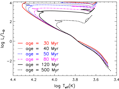
The precision of the recovery procedure was tested by building synthetic clusters with artificial stars sampled from the same PROSECCO isochrone grid used for the recovery procedure. A Gaussian noise with a standard deviation equal to the assumed observational uncertainties was added to the magnitude and colour values for each generated star. This numerical experiment showed the capability of the method to recover the simulated age and reddening in the ideal case where the adopted stellar models are in perfect agreement with real stars and the observational sample is populated with sufficient number of points.
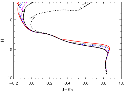
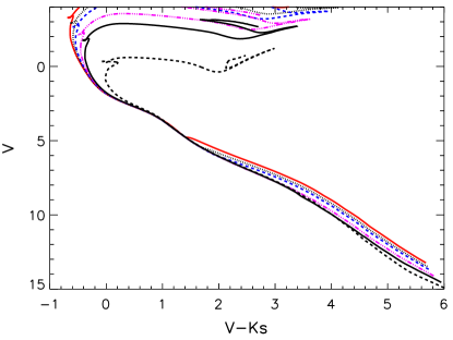
Figure 6 shows an example of PROSECCO isochrones of ages in the range of interest (30-500 Myr) in the different planes selected for the comparison with real clusters (as discussed in the following Section). Depending on the age and on the selected plane, different parts of the diagram are the main age indicators. In clusters younger than about 80-100 Myr low-mass stars are still sensitive to an age variation and are used to infer the age. For older clusters, low-mass stars are on the ZAMS and the age determination mainly relies on the brightest stars of the sample (if present).
We finally note that some of the sample clusters are characterised by very clean sequences, while others are more scattered, in spite of the Gaia and GES conservative membership analysis, suggesting that some contamination and/or large errors in photometry are still present. For each cluster, we tried to reduce the actual number of outliers using the cleaning procedure discussed in Appendix. B.
6 Results and discussion
6.1 Recovered ages and reddening values
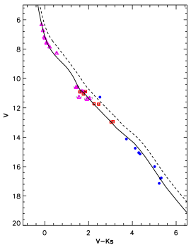
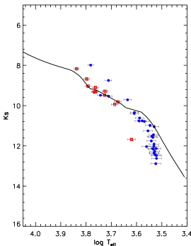
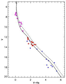
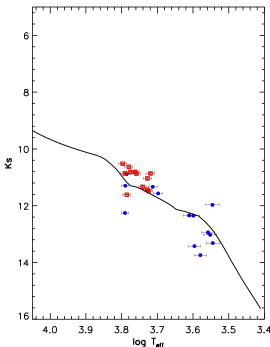
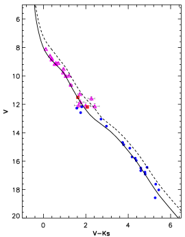
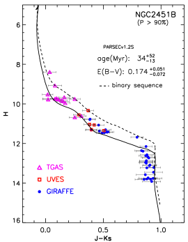
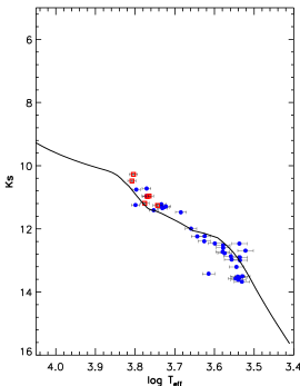
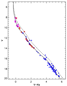
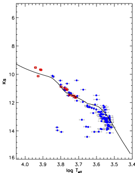
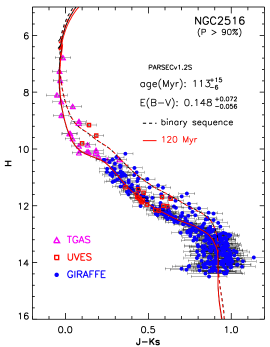
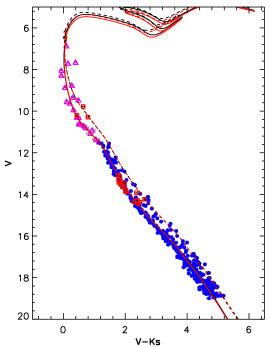
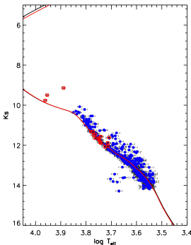
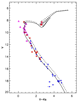
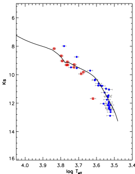
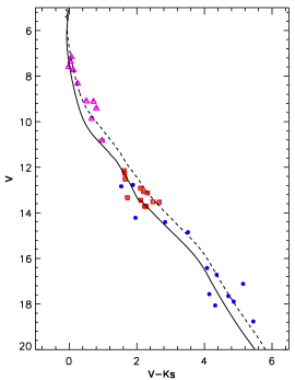
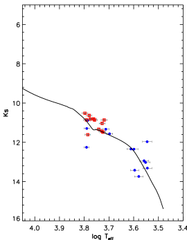
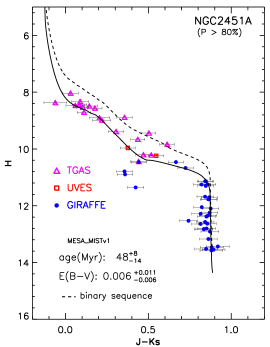
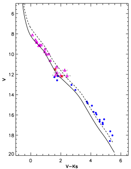
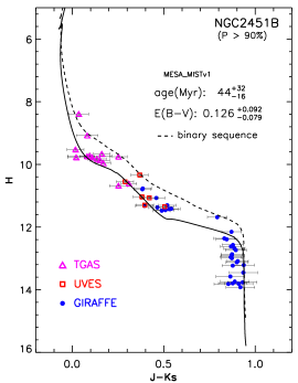
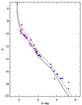
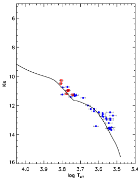
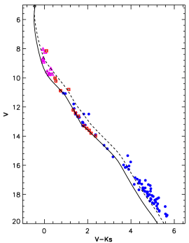
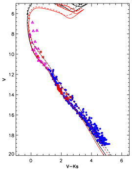
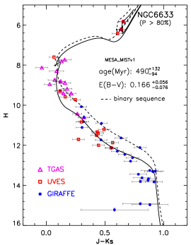
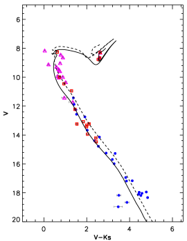
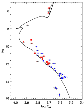
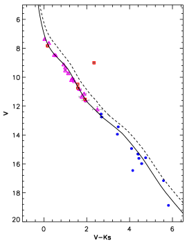
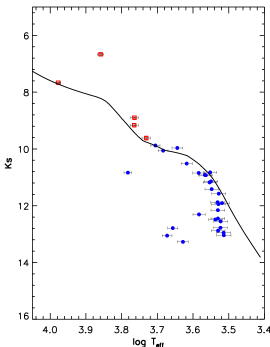
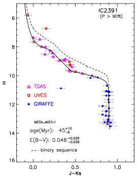
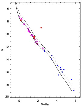
The most probable age and reddening values derived through our analysis are listed in Table 8 and are adopted to show the comparison between models and data in the (,), (,), and (, ) planes. Specifically, Figs. 7, 8, 9 and 10 show the CMDs and temperature-magnitude diagrams of selected relevant cases. The recovery has been performed for all the clusters with and without the inclusion of unresolved binaries and the derived ages and reddening in the two cases are consistent within the estimated uncertainties (for more details see Appendix B).


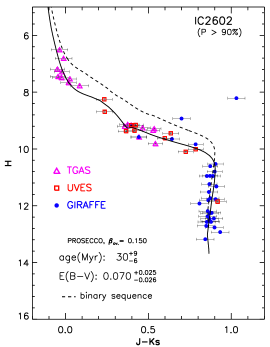
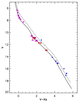

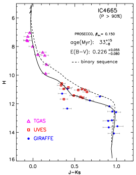
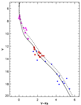
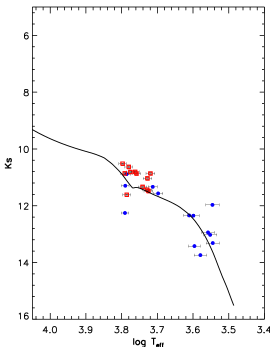


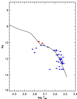
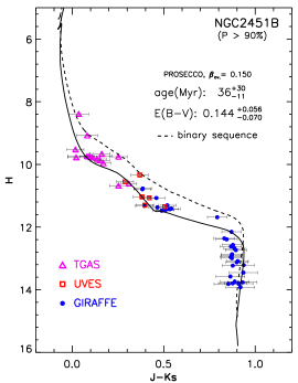
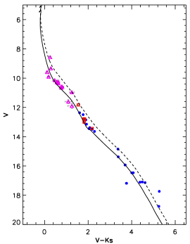
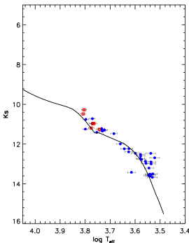

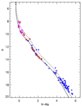
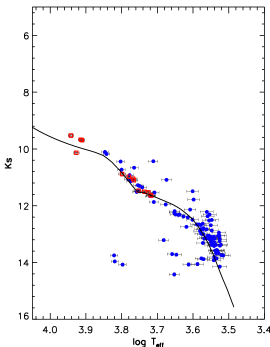
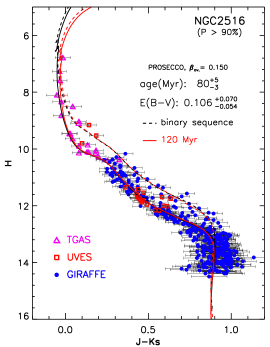
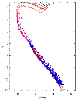


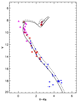

We first note that, as shown by Table 8, our procedure allowed us to recover ages with cumulative uncertainties between 5 and 30 %, with the exception of NGC 2451B, which is characterised by a much larger uncertainty, due to the combination of relatively large error in distance and small number of members. Also, the homogeneous analysis has enabled the establishment of an age ranking, which does not seem to depend on which model dataset was used, although there is some dependency on the magnitudes used for the recovery (see Sect. 6.2 below). More generally, the Figures show a good, global agreement between theory - isochrones with the most probable ages and reddening values - and observations for all the clusters. Noticeably, this is true for the different selected CMDs (for the entire sequences) and even in the Ks versus Teff diagrams. Some of the Figures suggest a tendency of the low-mass models to be somewhat bluer than the observations in the (, ) plane. Such a behaviour is not present if the colour or Teff are considered, indicating that at least part of the problem could be related to the adopted colour transformations, as already discussed in the literature (see e.g. Kučinskas et al., 2005; Casagrande & VandenBerg, 2014).
The two older clusters, NGC 2516 and NGC 6633, deserve some further comments. NGC 2516 (top panel of Fig. 10) is the cluster with the largest number of members among those analysed in the present work. Both the sequence of single stars and that of binaries of equal mass are clearly visible. In this cluster, low-mass stars are very close to their ZAMS position, weakly sensitive to age, which in principle should be mainly determined from stars close to the turn-off. Unfortunately, given the bright limit of both GES and available photometric surveys, relatively few members in that position () are present in the current sample. Also, while we identified 22 stars from TGAS, only a few of them are close to the turn-off; a few more may come from the stars identified in VL17, once these are confirmed to be members.
Finally, NGC 6633 (bottom panel of Fig. 10) is the only cluster in our sample with a few stars in the central helium burning phase, sensitive to the extension of the convective core during the MS phase. Thus, we derived age and reddening using two values of the core overshooting parameter, namely and 0.25. Due again to the small sample of stars close to the turn-off region and in the He-burning phase, the two models with different values of core overshooting are almost indistinguishable, both in terms of ages and reddening, although the case with seems to be favoured by a slightly better fit quality.
We evaluated the impact of a slightly different [Fe/H] on the age and reddening determination by running the analysis considering [Fe/H] for all the clusters. This value corresponds to the lowest metallicity listed in Table 2; that for NGC 2516. Adopting a different metallicity does result in changed estimates for the age and reddening. On the one hand, however, the metallicity of these clusters has been homogeneously measured by GES with good precision, and on the other hand, in the case of NGC 2516, with [Fe/H], we obtained a reduction in age of 1-2% and an increase in E of 0.02-0.03 mag. Similar numbers are found for the other clusters. This is a small effect, smaller than the currently estimated uncertainties, but will become more important when the systematic uncertainties in the Gaia parallaxes are removed.
| PROSECCO | PARSEC | MIST | ||||
|---|---|---|---|---|---|---|
| Cluster | (Myr) | E | (Myr) | E | (Myr) | E |
| NGC 2451A | ||||||
| NGC 2451B | ||||||
| NGC 2516 | ||||||
| NGC 2547 | ||||||
| IC 2391 | ||||||
| IC 2602 | ||||||
| IC 4665 | ||||||
| NGC 6633a | ||||||
| NGC 2451A | ||||||
| NGC 2451B | ||||||
| NGC 2516 | ||||||
| NGC 2547 | ||||||
| IC 2391 | ||||||
| IC 2602 | ||||||
| IC 4665 | ||||||
| NGC 6633a | ||||||
a in the PROSECCO models.


6.2 MIST and PARSEC models
In order to investigate the dependence of the recovered ages and reddening values on the adopted set of stellar models, we performed the same analysis using the PARSEC and MIST isochrones. The relevant sets of isochrones in the same age intervals used for PROSECCO were downloaded from the databases.
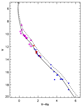
The age and reddening values obtained with the PARSEC and MIST models are listed in Table 8 together with the PROSECCO results. The table shows that with the exception of NGC 2516, the ages derived using the three model sets are in good agreement. The differences for the reddening are instead more significant; in particular, we note that MIST models and the analysis with the 2MASS magnitudes provide the lowest values, likely due to the fact that MIST isochrones for low-mass stars are slightly redder than the other two datasets in the versus plane.
The comparison of the full set of sample clusters with the MIST and PARSEC models is shown in Appendix. C; Fig 11 only shows the comparison between the data for IC 2391 and the PARSEC (top panel) and MIST (bottom panel) isochrones. The agreement between the models and observed stars in the 2MASS colour-magnitude diagrams appears good. PARSEC isochrones better reproduce the low-mass tail in the ( ) plane, while MIST models are bluer than data in this region. On the other hand, when the effective temperature is considered, MIST models appear in good agreement with observations, like the PROSECCO ones, while PARSEC isochrones show large deviations for . This is probably due to the modification introduced in the PARSEC models, discussed in Appendix A. The same deviation in the Teff plane found for low-mass stars when adopting PARSEC isochrones is present for all the analysed clusters.
As already mentioned, colours in the models (the PROSECCO and MIST ones at least) tend to be bluer than observations for low-mass stars (i.e., for magnitudes larger than about 16 in the selected clusters), thus possibly leading to a systematic effect in the derived age and reddening. In order to check the robustness of our procedure, we hence also made a test including in the recovery the Johnson magnitude together with the 2MASS bands. The results are shown in the bottom part of Table 8 for the three selected model sets. The inclusion of the band in the recovery procedure yields ages that are generally in agreement within their estimated uncertainties with those derived using only the 2MASS bands; formal errors in ages are generally smaller, because of the inclusion of an additional band (although with fewer points).
Concerning the recovered reddening, the E value is also sensitive to the use of the band in the recovery. However, generally, the derived E is compatible with that obtained in the 2MASS case, with the exception of NGC 2451A when the MIST and PROSECCO models are used. In this case, the derived reddening is much larger than that found using the 2MASS bands.
6.3 Comparison with the literature
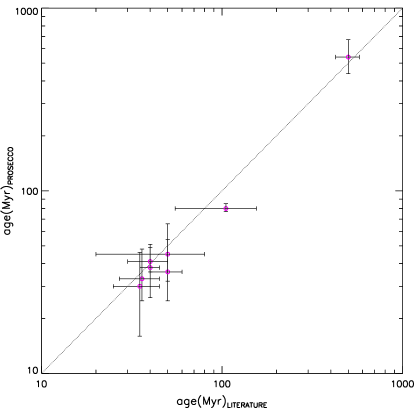
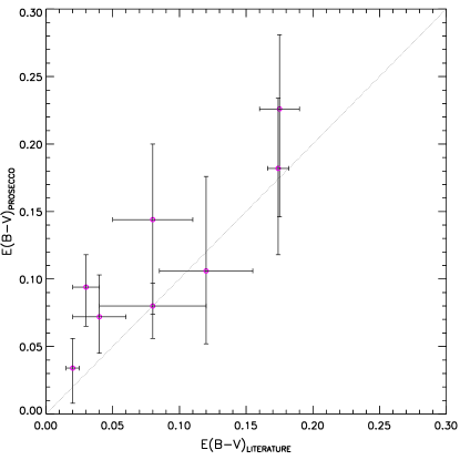
In Fig. 12 we plot our determination of ages and reddening obtained with the PROSECCO models and 2MASS magnitudes against literature values (see Table 1). For each cluster we show the average of the literature values and adopt the difference between the maximum and minimum values as error bars. The Figure suggests a general good agreement for the majority of the clusters, although the values derived by us are somewhat smaller than literature determinations. Independently from the absolute values of the ages, the relevant result here is that all the sample clusters have been analysed in a homogeneous way and are now on the same age scale. Our rigorous statistical approach also indicates that cluster ages are generally very solid against the chosen models; this represents an interesting result, which was not obvious a priori. As already noted, Table 8 shows that for all clusters, with the exception of NGC 2516 (which we discuss below), the ages recovered with the three sets of models are consistent within the errors, which have a significant contribution coming from the uncertainties in the cluster distances.
For some of the clusters the final cumulative errors on the ages are still larger than or comparable to those achieved in the literature using photometry only and leaving the distance as a free parameter (e.g. Cargile & James (2010) for IC 4665; Naylor & Jeffries (2006) for NGC 2547). As mentioned, the TGAS systematic error in parallax is several times larger than the random errors on the mean cluster parallaxes, it dominates the cumulative error in distance, and thus the age uncertainty.
| Cluster | ||
|---|---|---|
| (Myr) | (Myr) | |
| NGC2451A | ||
| NGC2451B | ||
| NGC2516 | ||
| NGC2547 | ||
| IC2391 | ||
| IC2602 | ||
| IC4665 | ||
| NGC6633 |
The next Gaia DR2 (April 2018) will include a consistent astrometric solution based on Gaia observations only, and the small-scale spatial variations of the parallax systematics are expected to be significantly reduced. In order to test how this will affect the uncertainty of the age recovery, we analysed a case in which we assume that the parallax/distance is known with better accuracy. Namely, if we reduce the adopted systematic uncertainty in the mean cluster parallax to only 0.1 mas, instead of 0.3 mas, we find that the systematic distance uncertainty becomes comparable to the current statistical uncertainty (or in the worst cases, still twice as large). We ran the parameter recovery process using this smaller total distance uncertainty for all the clusters. Table 9 shows the comparison between the original age uncertainties, determined when the 0.3 mas systematic distance error was considered (along with the random part and the photometric one), and the values obtained when a systematic error of 0.1 mas was adopted. The Table shows that for all the clusters, the age confidence intervals are significantly reduced, with the exception of NGC 2451B for which it is still not satisfactory. This test clearly confirms that distance uncertainty has a large impact on the final errors on ages; therefore, there is obvious room for a significant improvement of the results with the anticipated increase in the quality of Gaia parallaxes in subsequent data releases. In addition, the fainter magnitude limit of Gaia DR2 (astrometric parameters available down to mag instead of mag as for TGAS) will greatly increase the number of cluster members, which will help to significantly reduce the random errors and estimate more accurately the local systematic errors. Finally, precise homogeneous photometry available in Gaia DR2 will also contribute a significant improvement in the precision of the age estimates.
Focusing again on NGC 2516, the recovered ages using the PROSECCO and MIST models are younger by about 30% than commonly quoted values in the literature, while the ages from the PARSEC models are in better agreement with previous estimates. Figure 10 shows that the 120 Myr PROSECCO isochrone provides in principle a very good fit to the few stars at the turn-off. Indeed, we believe that the recovered age of Myr is driven by the stars close to the knee; whereas, as mentioned, these stars are less sensitive to age than stars close to the turn-off; they are much more numerous, hence amplifying the small age dependence. For the PROSECCO and MIST models, the 80 Myr isochrone is close in colour to the barycentre of those stars at the knee, while the same happens with the 100-120 Myr PARSEC isochrone. To better constrain the age for this cluster, we require either more stars at the turn-off region or more precise photometry for stars close to the knee.
We finally note that we performed an analysis of NGC 2516 adopting the parallax/distance of VL17, which corresponds to a smaller distance to the cluster. We derive an age of 80 Myr, but a very low reddening (E(); this is clearly far too small, hence supporting the larger distance derived by us.
The right-hand panel of Fig. 12 (see also Table 8) indicates that reddening is far less well constrained than age. Non-negligible differences are present with respect to the literature values (with our own estimates being generally larger) and our values are characterised by relatively large errors. Also the agreement between the results from the three models is less good than for the ages, with the MIST models generally providing values that are more similar to the literature ones. Part of the discrepancy between the reddening values derived here and those found in the literature might arise from the fact that the data used for the recovery mainly relies on near-infrared bands, which are less sensitive to the reddening. We believe that future analysis using Gaia photometry in the optical bands – which will be available for all cluster members – will allow improvement of this aspect.
6.4 Lithium depletion boundary ages
For the youngest clusters in our sample, a lithium depletion boundary (LDB) age determination has been performed in the literature. Given the very final goal of a consistent age calibration, which implies comparing cluster ages obtained with different methods, we again derive LDB ages here. We used our own estimates of the cluster distances, the PROSECCO models, and bolometric corrections, as well as the reddening values derived in this paper. LDB data have been retrieved from Jeffries & Oliveira (2005 -NGC 2547), Barrado y Navascués et al. (2004 –IC 2391), Dobbie et al. (2010 –IC 2602), and Manzi et al. (2008 –IC 4665), respectively. We note that the LDB age errors include the TGAS distance modulus uncertainty, but also an additional 0.1 mag uncertainty for photometric calibration (in colour and magnitude) and the likely uncertainty in the LDB location.
| Cluster | DM | E() | ()LDB | Age | |
|---|---|---|---|---|---|
| (mag) | (Myr) | ||||
| NGC 2547 | |||||
| IC 2391 | |||||
| IC 2602 | |||||
| IC 4665 |
LDB ages are shown in Table 10. Comparison with the ages reported in Table 8 suggests a good agreement; more specifically, the agreement is excellent for NGC 2547 and within for IC 2391 and IC 4665. This implies that by using the same set of models and assumptions, discrepancies between LDB and isochronal ages become less significant than previously claimed. The difference in inferred ages is somewhat larger for IC 2602, with the LDB age being more than 2 older than the isochronal one. In order to further check the age obtained with the Bayesian analysis, we tried to change (manually) the age of IC 2602 in the range 30-40 Myr. An age of more than about 32-33 Myr gets progressively less and less compatible with the data in the H versus , versus or versus Teff diagrams, and the isochrones reproduce only the lower envelope of the observed sequence. We also recall that an age around 30 Myr seems to be very robust even when adopting PARSEC or MIST models and/or including the -band. We note however that the recovery of the age for this cluster is mainly driven by the stars located in the region where there is a change of slope in the isochrones and where even a small difference in magnitude may lead to a significant difference in age. Whilst there are many stars at that position, they do not follow a very narrow sequence, but are relatively scattered, possibly due to the uncertainties in the 2MASS photometry. Also in this case, future Gaia releases will allow a more detailed analysis, possibly also indicating a front-to-back distance spread, given the proximity of the cluster.
7 Summary
We have homogeneously combined spectroscopic information from GES and Gaia-DR1 TGAS parallaxes for eight OCs, to derive a uniform set of cluster ages and reddening values, using a statistical Bayesian analysis applied to three different sets of standard evolutionary models. Parallaxes from TGAS data have been calculated and compared with the results of VL17. The agreement is good for all but one cluster, NGC 2516, for which we derive a smaller parallax (larger distance) than VL17. Both astrometric tests and the comparison with the isochrones support our own determination.
Our results show that the proposed approach is very promising. We have not only successfully tested our methodology, which will be further exploited with Gaia-DR2, but also the eight clusters have been put onto a consistent age scale for the first time. Although this ranking is model dependent, comparison of the results using the three different sets of models generally shows very good agreement, indicating that ages are robust against the chosen models for all but one cluster, NGC 2516. For this cluster, with two of the models (MIST and PROSECCO) we derived an age which is significantly younger than most values from the literature, while the PARSEC model provides an age in agreement with literature values. The younger age may be due to the lack of stars near the turn-off region, which prevents a robust age determination.
The LDB ages, determined in this paper for the four youngest clusters in the sample using the same evolutionary models (the PROSECCO ones), also generally agree well with isochronal ones. It has been claimed (Soderblom et al. 2014) that the LDB ages are far less model-dependent than ages determined from isochronal fits to high- or low-mass stars. It is therefore encouraging that three quarters of the clusters for which we have LDB and isochronal ages are in excellent agreement. E() values are instead less well constrained, since the Bayesian analysis has been performed using mainly near-infrared magnitudes that are not very sensitive to reddening.
Our analysis confirms that current errors in parallaxes, which are dominated by a relatively large systematic error, are a significant source of uncertainty in the derived ages (about 15-30%), especially in clusters with few and/or scattered photometric data. Indeed, ages and distances derived in the literature using photometry only can be more precise, but are not necessarily more accurate. We have quantitatively shown, however, how age uncertainties are expected to significantly improve once better Gaia parallaxes are available. Also, at this stage we cannot yet put extremely tight constraints on the models; nevertheless, we showed already that, among the chosen model sets, the PARSEC ones do not provide a good agreement with the observed sequences in the magnitude versus temperature diagrams.
Gaia-DR2, along with the full GES cluster dataset, will allow the extension of the present analysis to many more OCs, better sampling the age interval from a few Myr to several Gyr, and covering also metallicities above and below the solar value. The combination of Gaia proper motions with spectroscopic membership indicators will yield very clean sequences from the very bright down to the very faint stars. Extremely precise and homogeneous photometry from Gaia for virtually all cluster stars will also provide very valuable information. All this will allow more detailed comparisons with the models, including also those accounting for non-standard processes like rotation and magnetic fields, resulting in more crucial tests on the input physics. The dataset will not only enable tighter constraints on ages of our current sample and of many additional, more-distant clusters, but will also allow us to use that age information to calibrate a variety of commonly used age tracers, which, in turn, will allow estimates of the ages of field stars.
Acknowledgements.
Based on data products from observations made with ESO Telescopes at the La Silla Paranal Observatory under programme IDs 188.B-3002, 193.B.0936, and 197.B-1074. These data products have been processed by the Cambridge Astronomy Survey Unit (CASU) at the Institute of Astronomy, University of Cambridge, and by the FLAMES/UVES reduction team at INAF/Osservatorio Astrofisico di Arcetri. These data have been obtained from the Gaia-ESO Survey Data Archive, prepared and hosted by the Wide Field Astronomy Unit, Institute for Astronomy, University of Edinburgh, which is funded by the UK Science and Technology Facilities Council. This work has made use of data from the European Space Agency (ESA) mission Gaia (http://www.cosmos.esa.int/gaia), processed by the Gaia Data Processing and Analysis Consortium (DPAC, http://www.cosmos.esa.int/web/gaia/dpac/consortium). Funding for the DPAC has been provided by national institutions, in particular the institutions participating in the Gaia Multilateral Agreement. This research was made possible through the use of the AAVSO Photometric All-Sky Survey (APASS), funded by the Robert Martin Ayers Sciences Fundation. This research has made use of the SIMBAD and VizieR databases, operated at CDS, Strasbourg, France. This research has made use of NASA’s Astrophysics Data System. This work was partly supported by the European Union FP7 programme through ERC grant number 320360 and by the Leverhulme Trust through grant RPG-2012-541. We acknowledge the support from INAF and Ministero dell’ Istruzione, dell’ Università’ e della Ricerca (MIUR) in the form of the grant ”Premiale VLT 2012” and by PRIN-INAF 2014. The results presented here benefit from discussions held during the Gaia-ESO Survey workshops and conferences supported by the ESF (European Science Foundation) through the GREAT Research Network Programme. E.T., P.G.P.M. and S.D. acknowledge PRA Universitá di Pisa 2016 (Stelle di piccola massa: le pietre miliari dell’archeologia galattica, PI: S. Degl’Innocenti) and INFN (Iniziativa specifica TAsP). M.T.C acknowledge the financial support from the Spanish Ministerio de Economía y Competitividad, through grant AYA2016-75931. U.H. acknowledges support from the Swedish National Space Board (SNSB/Rymdstyrelsen). PRF and AS acknowledge useful discussions with Mario Lattanzi. We thank an anonymous referee for the very helpful and constructive comments.References
- Allard et al. (2011) Allard, F., Homeier, D., and Freytag, B. 2011, 16th Cambridge Workshop on Cool Stars, Stellar Systems, and the Sun, ASP Conference Series 448, 91
- Asplund et al. (2009) Asplund, M., Grevesse, N., Sauval, A. J., and Scott, P. 2009, ARA&A, 47, 481
- Balog et al. (2009) Balog, Z., Kiss, L.L., Vinkó, J., et al. 2009, ApJ, 698, 1989 A&A, 337, 403
- Baraffe et al. (2002) Baraffe, I., Chabrier, G., Allard, F., and Hauschildt, P. H. 2002, A&A, 382, 563
- Barrado y Navascués et al. (1999) Barrado y Navascués, D., Stauffer, J.R, and Patten, B.M 1999, ApJ, 522, L53
- Barrado y Navascués et al. (2004) Barrado y Navascués, D., Stauffer, J. R., and Jayawardhana, R. 2004, ApJ, 614, 386
- Bressan et al. (2012) Bressan, A., Marigo, P., Girardi, L., et al. 2012, MNRAS, 427, 127
- Burke et al. (2004) Burke, C. J., Pinsonneault, Marc. H., and Sills, A. 2004, ApJ, 604, 27
- Caffau et al. (2011) Caffau, E., Ludwig, H.-G., Steffen, M., Freytag, B., and Bonifacio, P. 2011, Solar Physics, 268, 255
- Cardelli et al. (1989) Cardelli, J. A., Clayton, G. C., and Mathis, J. S. 1989, ApJ,345, 245
- Cargile and James (2010) Cargile, P.A., and James, D.J., 2010, AJ, 140, 677
- Carrier et al. (1999) Carrier, F., Burki, G., and Richard, G. 2009, A&A, 341, 469
- Casagrande & VandenBerg (2014) Casagrande, L., and VandenBerg, D. A. 2014, MNRAS, 444, 392
- Castelli & Kurucz (2003) Castelli, F., and Kurucz, R. L. 2003, IAU Symposium, 210, 20
- Castelli (2005) Castelli, F. 2005, Mem. SAIt, 8, 25
- Chabrier & Baraffe (1997) Chabrier, G., and Baraffe, I. 1997, A&A, 327, 1039
- Charbonnel et al. (2013a) Charbonnel, C., Decressin, T., Amard, L., et al. 2013, A&A, 554, A40
- Chen et al. (2014) Chen, Y., Girardi, L., Bressan, A., Marigo, P., Barbieri, C., et al. 2014, MNRAS, 444, 2525
- Choi et al. (2016) Choi, J., Dotter, A., Conroy, C., Cantiello, M., Paxton, B., et al. 2016, ApJ, 823, 102
- Claria (1982) Claria, J. J. 1982, A&AS, 47, 323
- Damiani et al. (2014) Damiani F., Prisinzano, L., Micela, G., et al. 2014, A&A, 566, 50
- Cottaar et al. (2012) Cottaar, M., Meyer, M.R., and Parker, R.J. 2012, A&A, 547, 35
- Dell’Omodarme et al. (2012) Dell’Omodarme, M., Valle, G., Degl’Innocenti, S., and Prada Moroni, P. G. 2012, A&A, 540, 26
- Dias et al. (2002) Dias, W.S., Alessi, B. S., Moitinho, A. 2002, A&A, 389, 871
- Dobbie et al. (2010) Dobbie, P.D., Lodieu, N., and Sharp, R.G. 2010, MNRAS, 409, 1002
- Dotter (2016) Dotter, A. 2016, ApJS, 222, 8
- Eggenberger et al. (2010) Eggenberger, P., Meynet, G., Maeder, A., et al. 2010, A&A, 519, A116
- Feiden & Chaboyer (2012) Feiden, G. A. and Chaboyer, B. 2012, ApJ, 757, 42
- Feiden & Chaboyer (2014) Feiden, G. A. and Chaboyer, B. 2014, ApJ, 789, 53
- Feiden et al. (2015) Feiden, G. A., Jones, J., and Chaboyer, B. 2015, 18th Cambridge Workshop on Cool Stars, Stellar Systems, and the Sun, 18, 171
- Ferguson et al. (2005) Ferguson, J. W., Alexander, D. R., Allard, F., Barman, T., Bodnarik, et al. 2005, ApJ, 623, 585
- Gaia Collaboration et al. (2016a) Gaia collaboration, Prusti, T., de Brujine, J., et al. 2016, A&A, 595, A1
- Gaia Collaboration et al. (2016b) Gaia collaboration, Brown, A.G.A, Vallenari A., et al. 2016, A&A, 595, A2
- Gaia Collaboration et al. (2017) Gaia collaboration, van Leeuwen, F., Vallenari A., et al. 2017, A&A, in press
- Gennaro et al. (2012) Gennaro, M., Prada Moroni, P. G., and Tognelli, E. 2012, MNRAS, 420, 986
- Gilmore et al. (2012) Gilmore, G., Randich, S., Asplund, M., et al. 2012, The Messenger 147, 25
- Gurklyte, A. & Straizys, V. (1981) Gurklyte, A., and Straizys, V. 1981,57, 3
- Henden et al. (2016) Henden, A. A., Templeton, M., Terrell, et al. 2016, VizieR Online Data Catalog: AAVSO Photometric All Sky Survey (APASS) DR9
- Hill & Perry (1969) Hill, G., and Perry, C.L. 1969, AJ, 74, 1011
- Høg et al. (2000) Høg, E., Fabricius, C., Makarov, V.V., et al. 2000, A&A, 355, 27
- Hünsch et al. (2003) Hünsch, M., Weidner, C., and Schmitt, J.H.M.M. 2003, A&A, 402, 571
- Iglesias & Rogers (1996) Iglesias, C. A., and Rogers, F. J. 1996, ApJ, 464, 943
- Irwin (2008) Irwin, A. W. 2008, http://freeeos.sourceforge.net/
- Jackson & Jeffries (2014) Jackson, R. J., and Jeffries, R. D. 2014, MNRAS, 445, 4306
- Jackson et al. (2015) Jackson, R. J., Jeffries, R. D., Lewis, J., et al. 2015, A&A, 580, 75
- Jacobson et al. (2016) Jacobson, H.R., Friel, E. D., Jílkova, L., et al. 2016, A&A, 591, 37
- Jeffries et al. (1998) Jeffries, R.D., James, D. J., and Thurston, M.R. 1998, MNRAS, 300, 550
- Jeffries et al. (2004) Jeffries, R.D., Naylor, T., Devey, C.R., et al. 2004, MNRAS, 351, 1401.
- Jeffries & Oliveira (2005) Jeffries, R.D., and Oliveira J.M. 2005, MNRAS, 358,
- Jeffries et al. (2017) Jeffries, R. D., Jackson, R. J., Franciosini, E., et al. 2017, MNRAS, 464, 1456
- Jørgensen & Lindegren (2005) Jørgensen, B. R., and Lindegren, L. 2005, A&A, 436, 127
- Kharchenko & Roeser (2009) Kharchenko, N. V., and Roeser, S. 2009, VizieR Online Data Catalog, 128
- Kopytova et al. (2016) Kopytova, T. G., Brandner, W., Tognelli, E. Prada Moroni, P.G. Da Rio, N. et al. 2016, A&A, 585, 7
- Kučinskas et al. (2005) Kučinskas, A., Hauschildt, P. H., Ludwig, H.-G., et al. 2005, A&A, 442, 281
- Kurucz (1993) Kurucz, R. L. 1993, IAU Colloq. 138: Peculiar versus Normal Phenomena in A-type and Related Stars, 44, 87
- Lanzafame et al. (2015) Lanzafame, A. C., Frasca, A., Damiani, F., et al. 2015, A&A, 576, A80
- Lindegren et al. (2016) Lindegren, L., Lammers, U., Bastian, U., et al. 2016, A&A, 595, A4
- Lyra et al. (2006) Lyra, W., Moitinho, A., van der Bliek, N.S., and Alves, J. 2006, A&A, 453, 101
- Magrini et al. (2017) Magrini, L., Randich, S., Kordopatis, G., et al. 2017, A&A, 603, 2
- Manzi et al. (2008) Manzi, S., Randich, S. de Wit, W.J., and Palla, F. 2008, A&A, 479, 141
- Marigo et al. (2009) Marigo P., and Aringer B. 2009, A&A, 508, 1539
- Martin et al. (2007) Martin, N. F., Ibata, R. A., Chapman, S. C., Irwin, M., and Lewis, G. F. 2007, MNRAS, 380, 281
- Michalik et al. (2015) Michalik, D., Lindegren, L., and Hobbs, D. 2015, A&A, 574, 115
- Miglio et al. (2017) Miglio, A., Chiappini, C., Mosser, B., et al. 2017, AN, in press (arXiv:1706.03778)
- Montalbán et al. (2004) Montalbán, J., D’Antona, F., Kupka, F. and Heiter, U. 2004, A&A, 416, 1081
- Naylor & Jeffries (2006) Naylor, T., and Jeffries, R. D. 2006, MNRAS, 373, 1251
- Naylor (2009) Naylor, T. 2009, MNRAS 399, 432
- Nicolet (1981) Nicolet, B. 1981, A&A, 104, 185
- Palla et al. (2005) Palla, F., Randich, S., and Flaccomio, E. 2005, ApJ, 626, L49
- Pancino et al. (2017) Pancino, E., Lardo, C., Altavilla, G., et al. 2017, A&A, 598, 5
- Pasquini et al. (2002) Pasquini, L., Avila, G., Blecha, A., et al. 2002, Messenger, 110, 1
- Paunzen et al. (2014) Paunzen, E., Netopil, M. Maitzen, H. M., et al. 2014, A&A, 564, 42
- Paxton et al. (2011) Paxton, B., Bildsten, L., Dotter, A., et al. 2011, ApJS, 192, 3
- Paxton et al. (2013) Paxton, B., Cantiello, M., Arras, P. et al. 2013, ApJS, 208, 4
- Paxton et al. (2015) Paxton, B., Marchant, P., Schwab, J., et al. 2015, ApJS, 220, 15
- Platais et al. (2001) Platais, I., Kozhurina-Platais, V., Barnes, S., et al. 2001, AJ, 122, 1486
- Pryor & Meylan (1993) Pryor, C., and Meylan, G. 1993, Structure and Dynamics of Globular Clusters, 50, 357
- Raghavan et al. (2010) Raghavan, D., McAlister, H. A., and Henry, T. J. 2010, ApJS, 190, 1
- Randich et al. (2001) Randich, S., Pallavicini, R., Meola, G., et al. 2001, A&A, 377, 512
- Randich et al. (2013) Randich, S., Gilmore, G., and Gaia-ESO Consortium 2013, The Messenger 154, 47
- Rogers & Nayfonov (2002) Rogers, F. J., and Nayfonov, A. 2002, ApJ, 576, 1064
- Sacco et al. (2014) Sacco, G. G., Morbidelli, L., Franciosini, E., et al. 2014, A&A, 565, A113
- Sacco et al. (2015) Sacco, G. G., Jeffries, R. D., Randich, S., et al. 2015, A&A, 574, L7
- Salaris & Cassisi (2015) Salaris, M., and Cassisi, S. 2015, A&A, 577, A60
- Saumon et al. (1995) Saumon, D., Chabrier, G., and van Horn, H. M. 1995, ApJS, 99, 713
- Sestito & Randich (2005) Sestito, P. and Randich, S. 2005, A&A, 442, 615
- Siess (2001) Siess, L. 2001, ASP Conf. Series, 243, 581
- Silaj & Landstreet (2014) Silaj, J., and Landstreet, J. D.,A&A, 566, A132
- Skrutskie et al. (2006) Skrutskie, M.F., et al. 2006, AJ, 131, 1163
- Smiljanic et al. (2014) Smiljanic, R., Korn, A. J., Bergemann, M., et al. 2014, A&A, 570, A122
- Soderblom et al. (1993) Soderblom, D., Jones, B., and Balachandra, S. 1993, AJ, 106, 1059
- Soderblom (2010) Soderblom, D. 2010, ARA&A 48, 581
- Soderblom et al. (2014) Soderblom, D. , Hillenbrand, L.A., Jeffries, R.D., et al. 2014, Protostars and Planets VI, 219-241
- Somers & Pinsonneault (2015) Somers G., and Pinsonneault, M.H. 2015, MNRAS, 449, 4131
- Spina et al. (2017) Spina, L., Randich, S., Magrini, L., et al. 2017, A&A, 601, 70
- Stauffer et al. (1997) Stauffer, J. R., Hartmann, L. W., Prosser, C. F., et al. 1997, ApJ, 479, 776
- Sung et al. (2002) Sung, H., Bessell, M.S., Lee, B.-W., et al. 2002, AJ, 123, 290
- Tadross et al. (2002) Tadross, A.L, Werner, P., Osman, A., and Marie, M. 2002, New Astron., 7, 533
- Terndrup et al. (2002) Terndrup, D. M., Pinsonneault, M., Jeffries, R. D. et al. 2002, ApJ, 576, 950
- Tognelli et al. (2011) Tognelli, E., Prada Moroni, P. G., and Degl’Innocenti, S. 2011 A&A, 533, A109
- Tognelli et al. (2015a) Tognelli, E., Degl’Innocenti, S., Marcucci, L. E., and Prada Moroni P. G. 2015a, Physics Letter B, 742, 189
- Tognelli et al. (2015b) Tognelli, E., Prada Moroni, P. G., and Degl’Innocenti, S. 2015b, MNRAS, 449, 3741
- Trumpler & Weaver (1953) Trumpler R. J., and Weaver H. F. 1953, Statistical Astronomy (Dover Pubblications, Inc., New York)
- Valle et al. (2013) Valle, G., Dell’Omodarme, M., Prada Moroni, P. G., and Degl’Innocenti, S. 2013, A&A, 549, 50
- Valle et al. (2016) Valle G., Dell’Omodarme M., Prada Moroni P.G., and Degl’Innocenti S. 2016, A&A, 587, 16
- Valle et al. (2017) Valle, G., Dell’Omodarme, M., Prada Moroni, P. G. and Degl’Innocenti, S. 2017, A&A, 600, 41
- van Leeuwen (2009) van Leeuwen, F. 2009, A&A, 497, 209
- Viallet et al. (2015) Viallet, M., Meakin, C., Prat, V.,and Arnett, D. 2015, A&A, 580, 61
- Walker et al. (2006) Walker, M. G., Mateo, M., Olszewski, E. W., et al. 2006, AJ, 131, 2114
- Williams & Bolte (2007) Williams, K. A., and Bolte, M. 2007, AJ, 133, 1490
Appendix A Evolutionary Models
The main characteristics of the selected model grids are shown in Table 7. The selected stellar libraries have been computed adopting similar EOS, opacity, and solar mixture, while the atmospheric models used to specify the outer boundary conditions are different. This last quantity is particularly important in the case of low and very-low mass stars, where it can be responsible for relatively large deviations among models which adopt different BCs (see e.g. Tognelli et al. 2011).
Figure 13 compares solar composition isochrones of the selected sets for three ages in the range covered by the sample of observed OCs: 50 Myr, 100 Myr and 500 Myr. The comparison is made in the HRDs and in the CMDs in the photometric bands for which observational data are available (2MASS , , and Johnson bands). The Figure shows that in the HRD the PROSECCO and MIST isochrones below the turn-off are in excellent agreement among each other at all ages, while PARSEC isochrones are different from the other sets at low luminosities. This deviation is probably caused by an empirical recalibration of the atmospheric T relation adopted in the PARSEC models for T K () to reproduce the observed mass-radius relation (Chen et al. 2014). Such a recalibration seems to produce a large effect on the predicted Teff which gets significantly cooler than those of the other models at the same luminosity, reaching a maximum difference of 200-400 K at .
Near the turn-off region and in the central He burning phase the differences among the isochrones (mainly between PROSECCO/PARSEC and MIST) increase. However, in the age range we are dealing with, these two evolutionary phases are both sensitive also to the core overshooting efficiency during central hydrogen burning, which is different in the selected models.
The overshooting phenomenon, that is, the extension of the central mixing regions beyond the Schwarzschild border, , is generally parametrised in terms of the pressure scale height , where is a free parameter. For this comparison the PROSECCO models are calculated with . Note that PARSEC and MIST isochrones adopt a different treatment to estimate the core overshooting length . However, both formalisms are well reproduced by standard overshooting treatment if -0.25 is adopted (Bressan et al. 2012; Choi et al. 2016).
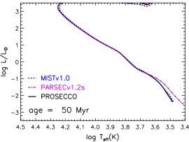
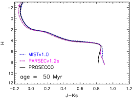
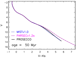
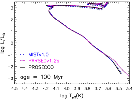
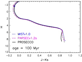
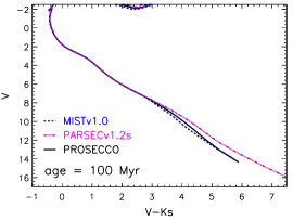
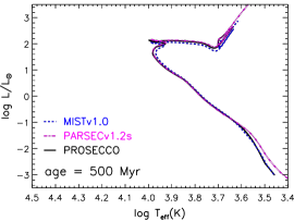
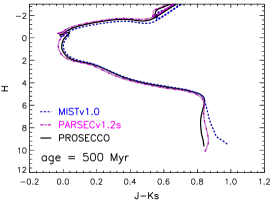
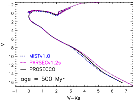
In our cluster sample only clusters with age of the order of or higher than 100 Myr include stars in the central hydrogen exhaustion region (turn-off) and in more advanced evolutionary phases (Red Giant Branch, RGB or central He burning). The CMDs show additional differences among the various sets with respect to the ones present in the HR diagram. This is due to the choice of synthetic spectra adopted to compute the bolometric corrections, required to convert luminosities into magnitudes. The differences in magnitude among the selected sets of isochrones vary with the chosen photometric system and with the stellar mass. In the (,) plane a maximum colour difference of about 0.04 mag (similar to typical photometric errors in the 2MASS CMDs of the selected clusters) is reached for the masses which populate the isochrone, with the exception of the low-mass stars tail, where the differences can exceed 0.1 mag. Similar differences are present in the (,) plane among the PROSECCO and MIST models, while the PARSEC ones can reach a colour difference of about 0.4 mag in the case of low-mass stars
Appendix B Cluster CMDs cleaning procedure and best models choice
As mentioned in the text, the CMDs of some of the analysed clusters are affected by contamination (field stars, unresolved binaries) even after the member selection process. Some of these stars, that have a membership probability higher than the imposed threshold, actually lie in regions of the CM diagrams incompatible neither with either a single star isochrone sequence, or with a plausible binary sequence. The presence of such outliers does not affect the final age and reddening determinations, but contributes with a large value to the total likelihood. Hence, we preferred to remove such objects from the sample used to derive the most probable age and reddening. However, in all the sample clusters the cleaning procedure removes a maximum of 3-4 objects which are those lying clearly below/above the cluster sequences and that can easily be identified by the reader.
The adopted cleaning procedure relies on four steps.
-
•
We identified the location of the ZAMS for each cluster. This has been done by comparing PROSECCO isochrones with data using the TGAS dereddened distance modulus and the average E available in the literature. We also checked that the adopted E value is compatible with the data for all the used photometric bands. Then, we identified the stars that have minimum distance from the single star ZAMS (above or below it) larger than and simultaneously in all the adopted photometric bands. These objects have been removed from the data sample used in the age analysis.
-
•
We ran the recovery procedure for the sample without the identified outliers, obtaining age and reddening values. We checked that the removed stars are outliers even adopting the new derived E (always verified). At this stage we did not include the unresolved binary sequence.
-
•
We used the age and reddening values to obtain the fiducial sequence. We built the unresolved binary sequence from such isochrone and we identified objects above the binary sequence with a minimum distance larger than (in all the used photometric bands). These stars have been removed.
-
•
We ran again the recovery with the new cleaned sample, including the unresolved binary sequence, and checked that the outliers still verify the distance conditions with the new derived age and reddening.
From such an analysis, we found that the derived age and reddening are not affected by the inclusion or exclusion of the outliers. The adoption of the cleaned sequence allows us to achieve a lower value (hence a larger likelihood). In addition, we checked that the most probable set actually reproduces the data and that, in the case of the inclusion of binaries, the fraction of stars within from the binary sequence is less than the stars within from the single star sequence. This is an empirical check to avoid that the single star sequence is less populated than the binary one, which would be unlikely.
Appendix C Cluster CMDs and temperature-magnitude diagrams
In this Section we show the comparison between the full sample of clusters but IC 2391 (previously shown in Sec. 5.2.2) and the PARSEC (Figs. 14-16) and MIST (Figs. 17-19) isochrones in the (, ), (,) and (Teff, ) diagrams.

