Asymptotically Minimax Robust Hypothesis Testing

Gökhan Gül
Fraunhofer Institute for Microengineering and Microsystems (IMM)
Carl-Zeiss-Str. 18-20, 55129 Mainz, Germany
Email: Goekhan.Guel@imm.fraunhofer.de
Abstract

The design of asymptotically minimax robust hypothesis testing is formalized for the Bayesian and Neyman-Pearson tests of Type-I and Type-II. The uncertainty classes based on the KL-divergence, α𝛼\alpha-divergence, symmetrized α𝛼\alpha-divergence, total variation distance, as well as the band model, moment classes and p-point classes are considered. Implications between single-sample-, all-sample- and asymptotic minimax robustness are derived. Existence and uniqueness of asymptotically minimax robust tests are proven using Sion’s minimax theorem and the Karush-Kuhn-Tucker multipliers. The least favorable distributions and the corresponding robust likelihood ratio functions are derived in parametric forms, which can then be determined by solving a system of equations. The proposed theory proves that Dabak’s design does not produce any asymptotically minimax robust test. Furthermore, it also generalizes the earlier works by Huber and Kassam by allowing analytical derivations, hence, providing answers to the questions ’how?’, which were left unanswered. Simulations are provided to exemplify and evaluate the theoretical derivations.

Index Terms:
Hypothesis testing, event detection, robustness, least favorable distributions, minimax optimization.

I Introduction

In simple binary hypothesis testing, complete statistical knowledge of the data is required in order to be able to design optimum tests [1]. However, such an assumption is too strict and often does not hold in practice [2]. In such a case a reasonable approach is to consider composite hypothesis represented by a set or class of distributions. Both the parametric [3, 4] as well as non-parametric approaches fall under this category [5]. While parametric models, including those driven by M-estimators [6], implicitly assume that the shape of the distributions is still perfectly known, non-parametric approaches, for example the sign- or the Wilcoxon test make only mild assumptions on the set of underlying distributions, hence they are regarded as conservative approaches [7].
Minimax robust hypothesis testing allows both parametric as well as non-parametric modeling of uncertainties by assuming that under the hypothesis jsubscript𝑗\mathcal{H}_{j} the true distribution Gjsubscript𝐺𝑗G_{j} of the received data belongs to an uncertainty class 𝒢jsubscript𝒢𝑗\mathscr{G}_{j}. The choice of the uncertainty classes is usually application dependent and most common choices are either model based, e.g. ϵitalic-ϵ\epsilon-contamination model, or distance based, e.g., uncertainty classes based on the KL-divergence [8]. Consequently, the ultimate goal of a designer is to find a decision rule δ^^𝛿\hat{\delta} which minimizes a predefined objective function for the least favorable distributions (LFDs) (G^0,G^1)𝒢0×𝒢1subscript^𝐺0subscript^𝐺1subscript𝒢0subscript𝒢1(\hat{G}_{0},\hat{G}_{1})\in\mathscr{G}_{0}\times\mathscr{G}_{1}. Under some mild conditions, such a design provides the most powerful test in a well defined minimax sense, i.e. a robust test which provides the best guaranteeable detection performance irrespective of uncertainties imposed on the statistical model.
Existence of minimax robust tests are completely determined by the choice of uncertainty sets. In case a minimax robust test does not exist over deterministic decision rules, it may still exist over the set of randomized decision rules [9]. The problem with such a design is that the designed test is minimax robust only for a single sample and cannot be extended to multiple samples while maintaining the minimax robustness [10]. In the presence of multiple samples and absence of minimax robust tests, probably the best option is to consider asymptotically minimax robust tests, which minimize the asymptotic decrease rate of the error probability. In summary, minimax robust tests can be broadly classified into four categories in terms of the number of samples or the choice of uncertainty classes:

  1. 1.

    All-sample minimax robust tests (over deterministic decision rules) [11, 12].

  2. 2.

    Single-sample minimax robust tests (over randomized decision rules) [8, 9, 10].

  3. 3.

    Asymptotically minimax robust tests (over deterministic decision rules) [13, 14].

  4. 4.

    Uncertainty classes defined on some probability space [7].

I-A Related work

The earliest work in robust hypothesis testing is attributed to P. J. Huber, who published a robust version of the probability ratio test for the ϵitalic-ϵ\epsilon-contamination and total variation classes of probability distributions in 1965 [11]. Huber derived the least favorable distributions and showed that the clipped likelihood ratio test was the minimax robust test for both uncertainty classes. The conclusions of this work was later extended by Huber and Strassen to a larger class, which includes five different classes as special cases [15]. The largest classes known, for which a minimax robust test exists and is a version of l^=g^1/g^0^𝑙subscript^𝑔1subscript^𝑔0\hat{l}=\hat{g}_{1}/\hat{g}_{0}, are the 222-alternating capacities [12], where g^jsubscript^𝑔𝑗\hat{g}_{j} is the density function corresponding to G^jsubscript^𝐺𝑗\hat{G}_{j}. All aforementioned works [11], [15] and [12] are all-sample minimax robust, and it was shown that such tests do not always exist, for example when the uncertainty classes are built with respect to the KL-divergence [16].
Clipped likelihood ratio tests (CLRTs) resulting from the uncertainty classes in [11] and [15] are widely used in practice, especially to deal with outliers. However, the models leading to CLRTs may be unrealistic for many applications, e.g., values of data samples which tend to infinity and still have a positive probability are almost never seen, but such a scenario is fully considered by the models in [11] and [15]. This was first observed by Dabak and Johnson, who suggested that eliminating such distributions could lead to a smoothed uncertainty model, which may be better suited for practical applications, where modeling errors is of interest. Based on this idea, they considered the KL-divergence as the distance to build the uncertainty classes and derived the corresponding robust test for the asymptotic case, i.e. as the number of measurements tends to infinity [13]. Under several assumptions, Levy showed that a single-sample minimax robust test could be designed for the same uncertainty model, if the error minimizing decision rules are allowed to be randomized. Considering a similar approach all the assumptions made by Levy were later removed [10]. The shortcomings of the model with the KL-divergence is that both the distance as well as the a priori probabilities of the nominal test are not selectable [10]. Replacing the KL-divergence with the α𝛼\alpha-divergence these two final constraints were also removed in [9]. Surprisingly, Dabak and Johnson’s asymptotically robust test was different from Levy’s minimax robust test, which was also different from the CLRT. Even more interestingly, for the whole α𝛼\alpha-divergence neighborhood and for any a priori probabilities of the hypotheses, the corresponding minimax robust test was a censored likelihood ratio test, with a well defined randomization function [9].
All aforementioned designs do not allow incorporating approximately known positions, shapes or statistics of the actual probability distributions into the considered model. Therefore, several other uncertainty models have been proposed in the literature. One approach is that the uncertainty classes can fully be defined in terms of the statistics of the actual distributions, such as the moments [14]. Another approach is to consider the p-point classes, which allow designation of the desired amount of area to the non-overlapping sub-sets of the domain of density functions [4, 17]. The band models, which was first proposed by Kassam [18] and later revisited by Fauß et. al. [19], on the other hand, enable the assignment of the approximate shape and location to the actual distributions.
All above-mentioned works in the field of robust hypothesis testing are theoretical. There are also application oriented works, for example [20], where Huber’s clipped likelihood ratio test is applied to robust detection of a known signal in nearly Gaussian noise. These results are later strengthened for a known signal in contaminated non-Gaussian noise [21]. Robust detection of stochastic signals for Gaussian signal and Gaussian mixture noise is also studied for small and large samples sizes [22]. Beside Huber’s uncertainty classes, moment classes have also been used in various applications, such as finance [23], admission control [24] and queueing theory [25]. P-point classes have been used in robust detection [4, 26], rate-distortion [27] and robust smoothing problems [28] whereas band models have been used in robust land mine detection [29], robust distributed detection [30], and robust and sequential gait symmetry detection [31]. In addition to direct detection procedures, robust detection has also been realized by means of robust estimation in radar applications considering complex elliptically symmetric distributions (CES) to model the clutter distribution [32, 33], see also [34] for a survey of the new results and applications.

I-B Motivation

  1. 1.

    The derivations in [13, 35], which are later summarized in [2], do not yield asymptotically minimax robust Neyman-Pearson (NP) tests. This requires derivations and analysis, which lead to minimax robustness.

  2. 2.

    The theoretical designs for the asymptotic case consider NP-formulations by default, probably because they result in simpler solutions [13, 14]. However, by Chernoff [36], it is well known that the NP-tests have the worst error exponents. Therefore, it is necessary to obtain the asymptotically minimax robust tests for the fastest decay rate of the error probability.

I-C Summary of the paper and its contributions

In this paper, the design of asymptotically minimax robust binary hypothesis tests is studied for various uncertainty classes. The existence and uniqueness of minimax robust tests are analyzed in general. Considering the Karush-Kuhn-Tucker (KKT) approach, the least favorable distributions and the robust likelihood ratio functions (LRFs) are derived in parametric forms, which can be made explicit by solving a set of non-linear equations. In the sequel, the contributions of this paper together with their relation to prior works are summarized.

  1. 1.

    It is shown that single-sample minimax robustness, hence all-sample minimax robustness (see Proposition III.4) implies asymptotically minimax robustness (see Proposition IV.4). The pillar of this work which makes most of other contributions possible is to show that any minimax robust test can be designed via solving

    minu(0,1)max(G0,G1)𝒢0×𝒢1Du(G0,G1),subscript𝑢01subscriptsubscript𝐺0subscript𝐺1subscript𝒢0subscript𝒢1subscript𝐷𝑢subscript𝐺0subscript𝐺1\min_{u\in(0,1)}\max_{(G_{0},G_{1})\in\mathscr{G}_{0}\times\mathscr{G}_{1}}D_{u}(G_{0},G_{1}),

    where

    Du(G0,G1)=Ωg1ug01u𝑑μsubscript𝐷𝑢subscript𝐺0subscript𝐺1subscriptΩsuperscriptsubscript𝑔1𝑢superscriptsubscript𝑔01𝑢differential-d𝜇D_{u}(G_{0},G_{1})=\int_{\Omega}{g_{1}}^{u}{g_{0}}^{1-u}d\mu

    is denoted as the u𝑢u-divergence. The corresponding test is single-sample minimax robust if there exists one. Otherwise the test is asymptotically minimax robust (see Section V).

  2. 2.

    For the KL-divergence neighborhood, the LFDs of the asymptotically minimax robust NP-tests of Type-I and Type-II are obtained in parametric forms. The parameters of LFDs can be found by solving four non-linear coupled equations and the corresponding test is different from the ones derived in [13, 35, 2] (see Theorem VI.2 and Remark VI.2).

  3. 3.

    For uncertainty classes based on the KL-divergence, α𝛼\alpha-divergence, symmetrized α𝛼\alpha-divergence, total variation distance as well as the band- and ϵitalic-ϵ\epsilon-contamination models, the LFDs of the (asymptotically) minimax robust rate minimizing tests are obtained in parametric forms. For moment classes and p-point classes, the design of minimax robust tests is defined as a convex optimization problem (see Section VI).

  4. 4.

    The derivations regarding the total variation neighborhood generalize the ones obtained earlier by Huber [11] via allowing unequal robustness parameters ϵ0ϵ1subscriptitalic-ϵ0subscriptitalic-ϵ1\epsilon_{0}\neq\epsilon_{1} to be chosen (see Theorem VI.5). Moreover, the analytical designs regarding the ϵitalic-ϵ\epsilon-contamination model, total variation neighborhood and the band model explain the choice of distributions and necessary parameters made by Huber [11] and Kassam [18], which were originally heuristically designed, i.e. the LFDs were some trial versions, which in turn yielded minimax robust tests. It is shown that two special cases of the band model give rise to two different versions of the ϵitalic-ϵ\epsilon-contamination model which accept the CLRT as the corresponding minimax robust test (see Theorem VI.6 and Theorem VI.8). It is also proven that both ϵitalic-ϵ\epsilon-contamination models are single-sample minimax robust (see [11] and Theorem VI.9) and their intersection yields the general version of the band model.

I-D Outline of the paper

The rest of the paper is organized as follows. In Section II, a brief overview of the fundamental concepts in minimax robust hypothesis testing is given. In Section III, single-sample and all-sample minimax robustness are defined. In Section IV, asymptotically minimax robustness is introduced and its relation to single- and all-sample minimax robustness is explained. In Section V, the equations formulating asymptotic minimax robustness are derived, saddle value condition is characterized and the problem statement is made. In Section VI, the least favorable distributions and asymptotically minimax robust tests are obtained for various uncertainty classes. In Section VII, simulations are performed to evaluate and exemplify the theoretical derivations. Finally in Section VIII, the paper is concluded.

I-E Notations

The following notations are applied throughout the paper. Upper case symbols are used for probability distributions and random variables, and the corresponding lower case symbols denote the density functions and observations, respectively. Boldface symbols are used for the sequence of random variables, sequence of observations or joint functions. The hypotheses 0subscript0\mathcal{H}_{0} and 1subscript1\mathcal{H}_{1} are associated with the nominal probability measures F0subscript𝐹0F_{0} and F1subscript𝐹1F_{1}, whereas the corresponding actual distributions are denoted by G0subscript𝐺0G_{0} and G1subscript𝐺1G_{1}. The sets of probability distributions are denoted by 𝒢0subscript𝒢0\mathscr{G}_{0} and 𝒢1subscript𝒢1\mathscr{G}_{1}, whereas \mathscr{M} is denoted as the set of all distribution functions on ΩΩ\Omega. Every probability measure, e.g. P[]𝑃delimited-[]P[\cdot], is associated with its distribution function P()𝑃P(\cdot) i.e., P(y)=P[Yy]𝑃𝑦𝑃delimited-[]𝑌𝑦P(y)=P[Y\leq y] for the random variable (r.v.) Y𝑌Y and the observation y𝑦y. The notation ()^^\hat{(\cdot)} indicates the least favorable distributions or densities, e.g., G^j𝒢jsubscript^𝐺𝑗subscript𝒢𝑗\hat{G}_{j}\in\mathscr{G}_{j}, or the most favorable decision rules e.g. δ^^𝛿\hat{\delta}. The expected value of a random variable Y𝑌Y is denoted by 𝔼[Y]𝔼delimited-[]𝑌\mathbb{E}[Y]. The notation for the convex function f𝑓f is different than the notation for the nominal density functions f0subscript𝑓0f_{0} or f1subscript𝑓1f_{1}, or the density functions fsubscript𝑓f_{\mathcal{L}} or f𝒩subscript𝑓𝒩f_{\mathcal{N}}, which correspond to the Laplacian and Gaussian density functions, respectively. Similarly, the likelihood ratio function denoted by l𝑙l has nothing in common with L0subscript𝐿0L_{0} or L1subscript𝐿1L_{1}, which correspond to the Lagrangians. The Lagrangian parameters μ0subscript𝜇0\mu_{0} and μ1subscript𝜇1\mu_{1} are also different from the notation used for the measure μ𝜇\mu. The symbols s0subscript𝑠0s_{0} and s0(λ1)subscript𝑠0subscript𝜆1s_{0}(\lambda_{1}) denote the same functions, where the latter is just explicitly written in terms of the unknown parameter. A𝐴A and Aksubscript𝐴𝑘A_{k} are defined as some sets belonging to the underlined sigma-algebra 𝒜𝒜\mathscr{A}. The argument (value on the domain) of the subsequent operation is denoted by arg\arg. The letter t𝑡t always indicates a threshold.

II Fundamentals of Minimax Robust Hypothesis Testing

Let (Yk)k1subscriptsubscript𝑌𝑘𝑘1(Y_{k})_{k\geq 1} be a sequence of independent and identically distributed (i.i.d.) random variables (r.v.s), each taking values on a measurable space (Ω,𝒜)Ω𝒜(\Omega,\mathscr{A}), where 𝒜𝒜\mathscr{A} is the Borel σ𝜎\sigma-algebra and ΩΩ\Omega is a set. Furthermore, let \mathscr{M} denote the set of all probability distribution functions defined on ΩΩ\Omega, and let 𝒢0subscript𝒢0\mathscr{G}_{0}\subset\mathscr{M} and 𝒢1subscript𝒢1\mathscr{G}_{1}\subset\mathscr{M} denote two distinct subsets of \mathscr{M}, each associated with the hypothesis 0subscript0\mathcal{H}_{0} and 1subscript1\mathcal{H}_{1}. The distribution of Yksubscript𝑌𝑘Y_{k} is not known exactly but belongs to the uncertainty set 𝒢jsubscript𝒢𝑗\mathscr{G}_{j} under the hypothesis jsubscript𝑗\mathcal{H}_{j}. The goal is to decide which of the following hypothesis is true

0subscript0\displaystyle\mathcal{H}_{0} :YkG0,G0𝒢0,:absentformulae-sequencesimilar-tosubscript𝑌𝑘subscript𝐺0subscript𝐺0subscript𝒢0\displaystyle:Y_{k}\sim G_{0},\quad G_{0}\in\mathscr{G}_{0},
1subscript1\displaystyle\mathcal{H}_{1} :YkG1,G1𝒢1.:absentformulae-sequencesimilar-tosubscript𝑌𝑘subscript𝐺1subscript𝐺1subscript𝒢1\displaystyle:Y_{k}\sim G_{1},\quad G_{1}\in\mathscr{G}_{1}. (1)

Given a sequence of observations 𝒚=(y1,,yn)𝒚subscript𝑦1subscript𝑦𝑛\bm{y}=(y_{1},\ldots,y_{n}) from either of the hypothesis, which corresponds to 𝒀=(Y1,,Yn)𝒀subscript𝑌1subscript𝑌𝑛\bm{Y}=(Y_{1},\ldots,Y_{n}), a statistical test (or a decision rule) is a measurable function δ:𝒀{0,1}:𝛿maps-to𝒀01\delta:\bm{Y}\mapsto\{0,1\}, which accepts the hypothesis δ(𝒚)subscript𝛿𝒚\mathcal{H}_{\delta(\bm{y})} and rejects the other. Let ΔΔ\Delta be the set of all δ𝛿\delta on ΩΩ\Omega, and P0=P(0)subscript𝑃0𝑃subscript0P_{0}=P(\mathcal{H}_{0}) and P1=P(1)subscript𝑃1𝑃subscript1P_{1}=P(\mathcal{H}_{1}) be the a priori probabilities of the hypotheses. Furthermore, let PF(δ,G0)=G0[δ(𝒀)=1]subscript𝑃𝐹𝛿subscript𝐺0subscript𝐺0delimited-[]𝛿𝒀1P_{F}(\delta,G_{0})=G_{0}[\delta(\bm{Y})=1] and PM(δ,G1)=G1[δ(𝒀)=0]subscript𝑃𝑀𝛿subscript𝐺1subscript𝐺1delimited-[]𝛿𝒀0P_{M}(\delta,G_{1})=G_{1}[\delta(\bm{Y})=0] define the false alarm and the miss detection probabilities, respectively, and

PE(δ,G0,G1)=P0PF(δ,G0)+P1PM(δ,G1)subscript𝑃𝐸𝛿subscript𝐺0subscript𝐺1subscript𝑃0subscript𝑃𝐹𝛿subscript𝐺0subscript𝑃1subscript𝑃𝑀𝛿subscript𝐺1P_{E}(\delta,G_{0},G_{1})=P_{0}P_{F}(\delta,G_{0})+P_{1}P_{M}(\delta,G_{1})

define the overall error probability. Then, a solution to the optimization problem

minδΔsup(G0,G1)𝒢0×𝒢1PE(δ,G0,G1)=sup(G0,G1)𝒢0×𝒢1minδΔPE(δ,G0,G1)subscript𝛿Δsubscriptsupremumsubscript𝐺0subscript𝐺1subscript𝒢0subscript𝒢1subscript𝑃𝐸𝛿subscript𝐺0subscript𝐺1subscriptsupremumsubscript𝐺0subscript𝐺1subscript𝒢0subscript𝒢1subscript𝛿Δsubscript𝑃𝐸𝛿subscript𝐺0subscript𝐺1\min_{\delta\in\Delta}\sup_{(G_{0},G_{1})\in{\mathscr{G}}_{0}\times{\mathscr{G}}_{1}}P_{E}(\delta,G_{0},G_{1})=\sup_{(G_{0},G_{1})\in{\mathscr{G}}_{0}\times{\mathscr{G}}_{1}}\min_{\delta\in\Delta}P_{E}(\delta,G_{0},G_{1}) (2)

is sought. The testing procedure and the distribution functions which solve (2) are called the minimax robust decision rule δ^^𝛿\hat{\delta} and the least favorable distribution functions (LFDs), G^0subscript^𝐺0\hat{G}_{0} and G^1subscript^𝐺1\hat{G}_{1}, respectively. The equality sign in (2), which is \geq in general, is not taken for granted and requires a careful analysis both on the objective function as well as on the uncertainty sets, for instance by using Sion’s minimax theorem [37]. A solution to (2) then implies a saddle value,

PE(δ^,G0,G1)PE(δ^,G^0,G^1)PE(δ,G^0,G^1).subscript𝑃𝐸^𝛿subscript𝐺0subscript𝐺1subscript𝑃𝐸^𝛿subscript^𝐺0subscript^𝐺1subscript𝑃𝐸𝛿subscript^𝐺0subscript^𝐺1P_{E}(\hat{\delta},G_{0},G_{1})\leq P_{E}(\hat{\delta},\hat{G}_{0},\hat{G}_{1})\leq P_{E}(\delta,\hat{G}_{0},\hat{G}_{1}). (3)

Given the densities g^0subscript^𝑔0\hat{g}_{0} and g^1subscript^𝑔1\hat{g}_{1} corresponding to the LFDs, G^0subscript^𝐺0\hat{G}_{0} and G^1subscript^𝐺1\hat{G}_{1}, the minimizing test δ^^𝛿\hat{\delta} is known to be the likelihood ratio test

𝒍^(𝒚)=k=1nl^(yk)01t^𝒍𝒚superscriptsubscriptproduct𝑘1𝑛^𝑙subscript𝑦𝑘superscriptsubscript0greater-than-or-equals-or-less-thansubscript1𝑡\hat{\bm{l}}(\bm{y})=\prod_{k=1}^{n}\hat{l}(y_{k})\stackrel{{\scriptstyle\mathcal{H}_{1}}}{{\underset{\mathcal{H}_{0}}{\gtreqless}}}t (4)

where l^=g^1/g^1^𝑙subscript^𝑔1subscript^𝑔1\hat{l}=\hat{g}_{1}/\hat{g}_{1} is the robust likelihood ratio function, 𝒍^^𝒍\hat{\bm{l}} is the joint robust likelihood ratio function and t𝑡t is a threshold. Depending on whether n=1𝑛1n=1, n<𝑛n<\infty or as n𝑛n\rightarrow\infty, analysis may differ. These cases and their interconnections will be handled in the next section. Uncertainty classes 𝒢0subscript𝒢0\mathscr{G}_{0} and 𝒢1subscript𝒢1\mathscr{G}_{1} will be made explicit whenever they are defined.

III Single-Sample and All-Sample Minimax Robustness

In the following single-sample minimax robustness is introduced. It is then extended to multiple samples. Existence and uniqueness of single-sample and finite-sample minimax robust tests are mentioned in this section and that of the asymptotic minimax robust test are presented more in details in the next sections.

Proposition III.1.

Let n=1𝑛1n=1 and Y=Y1𝑌subscript𝑌1Y=Y_{1}. If there exist LFDs, G^0𝒢0subscript^𝐺0subscript𝒢0\hat{G}_{0}\in\mathscr{G}_{0} and G^1𝒢1subscript^𝐺1subscript𝒢1\hat{G}_{1}\in\mathscr{G}_{1} such that

G0[l^(Y)<t]G^0[l^(Y)<t],subscript𝐺0delimited-[]^𝑙𝑌𝑡subscript^𝐺0delimited-[]^𝑙𝑌𝑡\displaystyle G_{0}\left[\hat{l}(Y)<t\right]\geq\hat{G}_{0}\left[\hat{l}(Y)<t\right],
G1[l^(Y)<t]G^1[l^(Y)<t],subscript𝐺1delimited-[]^𝑙𝑌𝑡subscript^𝐺1delimited-[]^𝑙𝑌𝑡\displaystyle G_{1}\left[\hat{l}(Y)<t\right]\leq\hat{G}_{1}\left[\hat{l}(Y)<t\right], (5)

for all t0𝑡subscriptabsent0t\in\mathbb{R}_{\geq 0} and all (G0,G1)𝒢0×𝒢1subscript𝐺0subscript𝐺1subscript𝒢0subscript𝒢1(G_{0},G_{1})\in\mathscr{G}_{0}\times\mathscr{G}_{1}, the corresponding test given by (4) solves (2) for the PEsubscript𝑃𝐸P_{E} minimizing t𝑡t.

Proof.

The proof is straightforward and is omitted, cf. [11, p. 1754]. ∎

Definition III.1 (Single-sample minimax robustness).

Existence of a single-sample minimax robust test stated by Proposition III.1 is called single-sample minimax robustness.

There is a tight connection between minimizing a distance and finding a solution to (III.1). This will be stated with the following theorem.

Theorem III.2.

Let G0subscript𝐺0G_{0} and G1subscript𝐺1G_{1} be two probability distributions which are both absolutely continuous with respect to a common measure μ𝜇\mu on ΩΩ\Omega. Then, for the f𝑓f-divergence [38] defined by

Df(G0,G1)=Ωf(g0g1)g1𝑑μ,subscript𝐷𝑓subscript𝐺0subscript𝐺1subscriptΩ𝑓subscript𝑔0subscript𝑔1subscript𝑔1differential-d𝜇D_{f}(G_{0},G_{1})=\int_{\Omega}f\left(\frac{g_{0}}{g_{1}}\right)g_{1}d\mu, (6)

where f:0:𝑓subscriptabsent0f:\mathbb{R}_{\geq 0}\to\mathbb{R} is a convex function such that f(1)=0𝑓10f(1)=0, we have

(G^0,G^1)𝒢0×𝒢1 satisfies (III.1)(G^0,G^1)𝒢0×𝒢1 minimizes Dfsubscript^𝐺0subscript^𝐺1subscript𝒢0subscript𝒢1 satisfies (III.1)subscript^𝐺0subscript^𝐺1subscript𝒢0subscript𝒢1 minimizes Df(\hat{G}_{0},\hat{G}_{1})\in\mathscr{G}_{0}\times\mathscr{G}_{1}\mbox{ satisfies \eqref{eq13x}}\Longleftrightarrow(\hat{G}_{0},\hat{G}_{1})\in\mathscr{G}_{0}\times\mathscr{G}_{1}\mbox{ minimizes $D_{f}$} (7)

over all (G0,G1)𝒢0×𝒢1subscript𝐺0subscript𝐺1subscript𝒢0subscript𝒢1(G_{0},G_{1})\in\mathscr{G}_{0}\times\mathscr{G}_{1} and for all twice continuously differentiable strictly convex functions f𝑓f, where the f𝑓f-divergence can alternatively be written as

Df(G0,G1)=0(min(1,t)Ωmin(g0,tg1)𝑑μ)𝑑μf(t)subscript𝐷𝑓subscript𝐺0subscript𝐺1superscriptsubscript01𝑡subscriptΩsubscript𝑔0𝑡subscript𝑔1differential-d𝜇differential-dsubscript𝜇𝑓𝑡D_{f}(G_{0},G_{1})=\int_{0}^{\infty}\left(\min(1,t)-\int_{\Omega}\min(g_{0},tg_{1})d\mu\right)d\mu_{f}(t) (8)

with

μf(a,b]=rf(b)rf(a),0<a<b<formulae-sequencesubscript𝜇𝑓𝑎𝑏superscript𝑟𝑓𝑏superscript𝑟𝑓𝑎0𝑎𝑏\mu_{f}(a,b]=\partial^{r}f(b)-\partial^{r}f(a),\quad 0<a<b<\infty

where rsuperscript𝑟\partial^{r} denotes the right derivative operator.

Proof:

The equivalence stated by (7) was proven in [12, Section 6]111In [12] ΩΩ\Omega is defined to be a complete separable metrizable space. Furthermore, if all (G0,G1)𝒢0×𝒢1subscript𝐺0subscript𝐺1subscript𝒢0subscript𝒢1(G_{0},G_{1})\in\mathscr{G}_{0}\times\mathscr{G}_{1} are absolutely continuous with respect to a fixed measure μ𝜇\mu, ΩΩ\Omega may need to be finite. for a version of Dfsubscript𝐷𝑓D_{f};

Df(G0,G1)=Ωf(g0g0+g1)(g0+g1)𝑑μ,subscript𝐷superscript𝑓subscript𝐺0subscript𝐺1subscriptΩsuperscript𝑓subscript𝑔0subscript𝑔0subscript𝑔1subscript𝑔0subscript𝑔1differential-d𝜇D_{f^{*}}(G_{0},G_{1})=\int_{\Omega}f^{*}\left(\frac{g_{0}}{g_{0}+g_{1}}\right)(g_{0}+g_{1})d\mu,

where f:[0,1]:superscript𝑓01f^{*}:[0,1]\to\mathbb{R} is a twice continuously differentiable and strictly convex function. Let f(y)=f(y)f(1/2)superscript𝑓absent𝑦superscript𝑓𝑦superscript𝑓12f^{**}(y)=f^{*}(y)-f^{*}(1/2) which results in f(1/2)=0superscript𝑓absent120f^{**}(1/2)=0. By [39, Equation 7,8], it is known that Df=Dfsubscript𝐷𝑓subscript𝐷superscript𝑓absentD_{f}=D_{f^{**}} using the transformation f(t)=tf((1t)/t)superscript𝑓absent𝑡𝑡𝑓1𝑡𝑡f^{**}(t)=tf((1-t)/t) for t(0,1)𝑡01t\in(0,1). Hence, minimizing Dfsubscript𝐷𝑓D_{f} and Dfsubscript𝐷superscript𝑓absentD_{f^{**}} are equivalent over all twice continuously differentiable and strictly convex f𝑓f. An alternative definition of Dfsubscript𝐷𝑓D_{f} given by (8) can be found in [40, Equation 10]. ∎

Depending on the definition of the uncertainty classes, 𝒢0subscript𝒢0\mathscr{G}_{0} and 𝒢1subscript𝒢1\mathscr{G}_{1}, a minimax robust test may or may not exist. For example it exists for the ϵitalic-ϵ\epsilon-contamination classes of distributions [11] and it does not exist for the classes of distributions based on the KL-divergence [16]. If the uncertainty classes do not allow a minimax robust test to exist for all thresholds, it may still be possible to obtain a minimax robust test for a unique decision rule, if randomized decision rules are allowed, see [16]. The information in the randomization is lost by the multiplication of the likelihood ratios therefore straightforward extension of the test to multiple observations is not minimax robust. However, if a single-sample minimax robust test exists, then it also implies existence of a finite-sample minimax robust test for any n<𝑛n<\infty. In order to prove this, let us first consider the following definition and lemma.

Definition III.2.

Let X𝑋X and Y𝑌Y be two random variables taking values on the same measurable space (Ω,𝒜)Ω𝒜(\Omega,{\mathscr{A}}), having cumulative distribution functions G0subscript𝐺0G_{0} and G1subscript𝐺1G_{1}, respectively. X𝑋X is called stochastically larger than Y𝑌Y, i.e. XYsucceeds-or-equals𝑋𝑌X\succeq Y, if G1(x)G0(x)subscript𝐺1𝑥subscript𝐺0𝑥G_{1}(x)\geq G_{0}(x) for all x𝑥x.

Lemma III.3.

Let X1subscript𝑋1X_{1}, X2subscript𝑋2X_{2}, Y1subscript𝑌1Y_{1} and Y2subscript𝑌2Y_{2} be four random variables on (Ω,𝒜)Ω𝒜(\Omega,{\mathscr{A}}), out of which X1subscript𝑋1X_{1} and X2subscript𝑋2X_{2}, and Y1subscript𝑌1Y_{1} and Y2subscript𝑌2Y_{2} are independent. If X1Y1succeeds-or-equalssubscript𝑋1subscript𝑌1X_{1}\succeq Y_{1} and X2Y2succeeds-or-equalssubscript𝑋2subscript𝑌2X_{2}\succeq Y_{2}, then X1+X2Y1+Y2succeeds-or-equalssubscript𝑋1subscript𝑋2subscript𝑌1subscript𝑌2X_{1}+X_{2}\succeq Y_{1}+Y_{2}.

Proof:

Proof of Lemma (III.3) is simple and is omitted. ∎

Proposition III.4.

If a single-sample minimax robust test exists, then a minimax robust test exists for any finite-sample size n<𝑛n<\infty with the same LFDs and for the same uncertainty classes.

Proof:

If l^(Y)^𝑙𝑌\hat{l}(Y) satisfies the inequalities in (III.1), so does Xk=logl^(Yk)subscript𝑋𝑘^𝑙subscript𝑌𝑘X_{k}=\log\hat{l}(Y_{k}) for all k𝑘k, but for all t𝑡t\in\mathbb{R}. Application of Lemma III.3 to the sum of n𝑛n r.v.s implies that k=1nXksuperscriptsubscript𝑘1𝑛subscript𝑋𝑘\sum_{k=1}^{n}X_{k} is stochastically larger under G^0subscript^𝐺0\hat{G}_{0} than under G0subscript𝐺0G_{0}, and similarly under G1subscript𝐺1G_{1} than under G^1subscript^𝐺1\hat{G}_{1}. Hence, by Definition III.2 we have

G0[k=1nXkt]G^0[k=1nXkt],subscript𝐺0delimited-[]superscriptsubscript𝑘1𝑛subscript𝑋𝑘𝑡subscript^𝐺0delimited-[]superscriptsubscript𝑘1𝑛subscript𝑋𝑘𝑡\displaystyle G_{0}\left[\sum_{k=1}^{n}X_{k}\leq t\right]\geq\hat{G}_{0}\left[\sum_{k=1}^{n}X_{k}\leq t\right],
G1[k=1nXkt]G^1[k=1nXkt]subscript𝐺1delimited-[]superscriptsubscript𝑘1𝑛subscript𝑋𝑘𝑡subscript^𝐺1delimited-[]superscriptsubscript𝑘1𝑛subscript𝑋𝑘𝑡\displaystyle G_{1}\left[\sum_{k=1}^{n}X_{k}\leq t\right]\leq\hat{G}_{1}\left[\sum_{k=1}^{n}X_{k}\leq t\right] (9)

for all t𝑡t and all (G0,G1)𝒢0×𝒢1subscript𝐺0subscript𝐺1subscript𝒢0subscript𝒢1(G_{0},G_{1})\in\mathscr{G}_{0}\times\mathscr{G}_{1}. This proves the assertion since

{exp(k=1nXk)exp(t)}{𝒍^(𝒀)t}.superscriptsubscript𝑘1𝑛subscript𝑋𝑘𝑡^𝒍𝒀superscript𝑡\left\{\exp\left(\sum_{k=1}^{n}X_{k}\right)\leq\exp(t)\right\}\equiv\{\hat{\bm{l}}(\bm{Y})\leq t^{{}^{\prime}}\}. (10)

Definition III.3 (All-sample minimax robustness).

Existence of minimax robust tests for any finite-sample size n<𝑛n<\infty stated by Proposition III.4 is called all-sample minimax robustness.

Remark III.1.

Proposition III.4 implies

Single-sample minimax robustnessAll-sample minimax robustnessSingle-sample minimax robustnessAll-sample minimax robustness\text{Single-sample minimax robustness}\Longleftrightarrow\mbox{All-sample minimax robustness}

Notice that in fact (Yk)k1subscriptsubscript𝑌𝑘𝑘1(Y_{k})_{k\geq 1} are required to be only independent but not necessarily identically distributed. This allows different uncertainty classed to be considered for each Yksubscript𝑌𝑘Y_{k}.

Existence of finite-sample minimax robust tests are established by Proposition III.4. Examples of such tests can be found in [15, 12]. However, as shown before, such tests may not always exist even for very simple examples. In this case a minimax robust test can be designed asymptotically as n𝑛n\rightarrow\infty. Asymptotically minimax robust hypothesis testing will be introduced in the next section. Uniqueness of minimax robust finite-sample tests are postponed to the next sections, due to the ease of derivations using the asymptotic theory.

IV Asymptotically Minimax Robustness

If the uncertainty model of interest does not allow all-sample minimax robustness, an asymptotic design is necessary. In the sequel, asymptotic minimax robustness will be formalized with first deriving the minimax equations, then, stating the existence of a saddle value and last, with a clear statement of the problem.

Definition IV.1 (Asymptotically minimax robustness).

Let Sn(𝑿)=1nlog𝒍^(𝑿)subscript𝑆𝑛𝑿1𝑛^𝒍𝑿S_{n}(\bm{X})=\frac{1}{n}\log\hat{\bm{l}}(\bm{X}). Then, the tests satisfying

limn1nlogG0[Sn(𝑿)>t]limn1nlogG^0[Sn(𝑿)>t]subscript𝑛1𝑛subscript𝐺0delimited-[]subscript𝑆𝑛𝑿𝑡subscript𝑛1𝑛subscript^𝐺0delimited-[]subscript𝑆𝑛𝑿𝑡\displaystyle\lim_{n\rightarrow\infty}\frac{1}{n}\log G_{0}\left[S_{n}(\bm{X})>t\right]\leq\lim_{n\rightarrow\infty}\frac{1}{n}\log\hat{G}_{0}\left[S_{n}(\bm{X})>t\right]
limn1nlogG1[Sn(𝑿)t]limn1nlogG^1[Sn(𝑿)t]subscript𝑛1𝑛subscript𝐺1delimited-[]subscript𝑆𝑛𝑿𝑡subscript𝑛1𝑛subscript^𝐺1delimited-[]subscript𝑆𝑛𝑿𝑡\displaystyle\lim_{n\rightarrow\infty}\frac{1}{n}\log G_{1}\left[S_{n}(\bm{X})\leq t\right]\leq\lim_{n\rightarrow\infty}\frac{1}{n}\log\hat{G}_{1}\left[S_{n}(\bm{X})\leq t\right]

for a fixed t𝑡t and for all (G0,G1)𝒢0×𝒢1subscript𝐺0subscript𝐺1subscript𝒢0subscript𝒢1(G_{0},G_{1})\in\mathscr{G}_{0}\times\mathscr{G}_{1} are called asymptotically minimax robust with respect to the chosen t𝑡t.

IV-A Derivation of the Rate Functions

Theorem IV.1.

Let 𝐘=(Y1,,Yn)𝐘subscript𝑌1subscript𝑌𝑛\bm{Y}=(Y_{1},\ldots,Y_{n}) be a sequence of i.i.d. r.v.s, where each Yksubscript𝑌𝑘Y_{k} is distributed as Gj𝒢jsubscript𝐺𝑗subscript𝒢𝑗G_{j}\in\mathscr{G}_{j} under jsubscript𝑗\mathcal{H}_{j}. Furthermore, let 𝐗=(X1,,Xn)𝐗subscript𝑋1subscript𝑋𝑛\bm{X}=(X_{1},\ldots,X_{n}) be the sequence of r.v.s induced by the robust log-likelihood ratios Xk:=logl^(Yk)assignsubscript𝑋𝑘^𝑙subscript𝑌𝑘X_{k}:=\log\hat{l}(Y_{k}), where each Xksubscript𝑋𝑘X_{k} has a finite moment generating function

MXkj(u)=𝔼Gj[exp(uXk)]<,j{0,1}.formulae-sequencesuperscriptsubscript𝑀subscript𝑋𝑘𝑗𝑢subscript𝔼subscript𝐺𝑗delimited-[]𝑢subscript𝑋𝑘𝑗01M_{X_{k}}^{j}(u)=\mathbb{E}_{G_{j}}\left[\exp\left({uX_{k}}\right)\right]<\infty,\quad j\in\{0,1\}. (11)

For the test comparing Sn(𝐗)=1nk=1nXksubscript𝑆𝑛𝐗1𝑛superscriptsubscript𝑘1𝑛subscript𝑋𝑘{S_{n}(\bm{X})=\frac{1}{n}\sum_{k=1}^{n}X_{k}} to a threshold t𝑡t, if

𝔼G0[Xk]<t<𝔼G1[Xk],subscript𝔼subscript𝐺0delimited-[]subscript𝑋𝑘𝑡subscript𝔼subscript𝐺1delimited-[]subscript𝑋𝑘\mathbb{E}_{G_{0}}[X_{k}]<t<\mathbb{E}_{G_{1}}[X_{k}], (12)

then, as n𝑛n\to\infty, false alarm and miss detection probabilities decrease exponentially

limn1nlogG0[Sn(𝑿)>t]=I0(t)subscript𝑛1𝑛subscript𝐺0delimited-[]subscript𝑆𝑛𝑿𝑡subscript𝐼0𝑡\displaystyle\lim_{n\rightarrow\infty}\frac{1}{n}\log G_{0}[S_{n}(\bm{X})>t]=-I_{0}(t) (13)
limn1nlogG1[Sn(𝑿)t]=I1(t)subscript𝑛1𝑛subscript𝐺1delimited-[]subscript𝑆𝑛𝑿𝑡subscript𝐼1𝑡\displaystyle\lim_{n\rightarrow\infty}\frac{1}{n}\log G_{1}[S_{n}(\bm{X})\leq t]=-I_{1}(t) (14)

with the rate functions given by

Ij(t)=supu(tulogMXkj(u)),j{0,1}.formulae-sequencesubscript𝐼𝑗𝑡subscriptsupremum𝑢𝑡𝑢superscriptsubscript𝑀subscript𝑋𝑘𝑗𝑢𝑗01I_{j}(t)=\sup_{u\in\mathbb{R}}\left(tu-\log M_{X_{k}}^{j}(u)\right),\quad j\in\{0,1\}. (15)
Proof:

The results ((13) and (14), respectively) follow by applying Cramér’s theorem [41] twice, first under 0subscript0\mathcal{H}_{0} to the sequence of r.v.s (Xk)k1subscriptsubscript𝑋𝑘𝑘1(X_{k})_{k\geq 1}, each satisfying 𝔼G0[Xk]<tsubscript𝔼subscript𝐺0delimited-[]subscript𝑋𝑘𝑡\mathbb{E}_{G_{0}}[X_{k}]<t, and second under 1subscript1\mathcal{H}_{1} to the sequence of r.v.s (Xk)k1subscriptsubscript𝑋𝑘𝑘1(-X_{k})_{k\geq 1}, each satisfying t<𝔼G1[Xk]𝑡subscript𝔼subscript𝐺1delimited-[]subscript𝑋𝑘t<\mathbb{E}_{G_{1}}[X_{k}]. The details of the proof can be found in [7, p. 84], [2, pp. 76-80]. ∎

Corollary IV.2.

Any of the following conditions is sufficient for (12) to hold.

  1. 1.

    There are G^0𝒢0subscript^𝐺0subscript𝒢0\hat{G}_{0}\in\mathscr{G}_{0} and G^1𝒢1subscript^𝐺1subscript𝒢1\hat{G}_{1}\in\mathscr{G}_{1} satisfying single-sample minimax robustness

  2. 2.

    𝔼G^1[Xk]<𝔼G1[Xk]subscript𝔼subscript^𝐺1delimited-[]subscript𝑋𝑘subscript𝔼subscript𝐺1delimited-[]subscript𝑋𝑘\mathbb{E}_{\hat{G}_{1}}[X_{k}]<\mathbb{E}_{G_{1}}[X_{k}] and 𝔼G^0[Xk]>𝔼G0[Xk]subscript𝔼subscript^𝐺0delimited-[]subscript𝑋𝑘subscript𝔼subscript𝐺0delimited-[]subscript𝑋𝑘\mathbb{E}_{\hat{G}_{0}}[X_{k}]>\mathbb{E}_{G_{0}}[X_{k}] for all (G0,G1)𝒢0×𝒢1subscript𝐺0subscript𝐺1subscript𝒢0subscript𝒢1(G_{0},G_{1})\in\mathscr{G}_{0}\times\mathscr{G}_{1}

  3. 3.

    min𝔼G1[Xk]>max𝔼G0[Xk]subscript𝔼subscript𝐺1delimited-[]subscript𝑋𝑘subscript𝔼subscript𝐺0delimited-[]subscript𝑋𝑘\min\mathbb{E}_{G_{1}}[X_{k}]>\max\mathbb{E}_{G_{0}}[X_{k}] for all (G0,G1)𝒢0×𝒢1subscript𝐺0subscript𝐺1subscript𝒢0subscript𝒢1(G_{0},G_{1})\in\mathscr{G}_{0}\times\mathscr{G}_{1}

Here we have 12121\Longrightarrow 2 and 23232\Longrightarrow 3 and the converses of these implications are not true in general.

Remark IV.1.

Even if none of the sufficient conditions listed above holds, it may still be possible to obtain an asymptotically minimax robust test. Let two disjoint subsets be A0×A1𝒢0×𝒢1subscript𝐴0subscript𝐴1subscript𝒢0subscript𝒢1A_{0}\times A_{1}\subset\mathscr{G}_{0}\times\mathscr{G}_{1} and B0×B1𝒢0×𝒢1subscript𝐵0subscript𝐵1subscript𝒢0subscript𝒢1B_{0}\times B_{1}\subset\mathscr{G}_{0}\times\mathscr{G}_{1}, where A0×A1B0×B1=𝒢0×𝒢1subscript𝐴0subscript𝐴1subscript𝐵0subscript𝐵1subscript𝒢0subscript𝒢1A_{0}\times A_{1}\cup B_{0}\times B_{1}=\mathscr{G}_{0}\times\mathscr{G}_{1}. Suppose that for all (G0,G1)A0×A1subscript𝐺0subscript𝐺1subscript𝐴0subscript𝐴1(G_{0},G_{1})\in A_{0}\times A_{1}, (12) holds and for all (G0,G1)B0×B1subscript𝐺0subscript𝐺1subscript𝐵0subscript𝐵1(G_{0},G_{1})\in B_{0}\times B_{1} we have 𝔼G1[Xk]<t<𝔼G0[Xk]subscript𝔼subscript𝐺1delimited-[]subscript𝑋𝑘𝑡subscript𝔼subscript𝐺0delimited-[]subscript𝑋𝑘\mathbb{E}_{G_{1}}[X_{k}]<t<\mathbb{E}_{G_{0}}[X_{k}]. Furthermore, suppose that either of the conditions

  1. 1.

    Whether (G0,G1)subscript𝐺0subscript𝐺1(G_{0},G_{1}) belongs to A0×A1subscript𝐴0subscript𝐴1A_{0}\times A_{1} or B0×B1subscript𝐵0subscript𝐵1B_{0}\times B_{1} is known to the decision maker.

  2. 2.

    Increasing behavior of error probability is instantly detectable.

is true. Then, flipping the binary decisions for all (G0,G1)B0×B1subscript𝐺0subscript𝐺1subscript𝐵0subscript𝐵1(G_{0},G_{1})\in B_{0}\times B_{1} (or whenever increasing PEsubscript𝑃𝐸P_{E} is detected) and keeping the original decisions for (G0,G1)A0×A1subscript𝐺0subscript𝐺1subscript𝐴0subscript𝐴1(G_{0},G_{1})\in A_{0}\times A_{1} allow the convergence of error probability to zero asymptotically for all (G0,G1)𝒢0×𝒢1subscript𝐺0subscript𝐺1subscript𝒢0subscript𝒢1(G_{0},G_{1})\in\mathscr{G}_{0}\times\mathscr{G}_{1}. However, in this case two different robust tests may need to be designed. Notice that for the flipped decisions I0subscript𝐼0I_{0} and I1subscript𝐼1I_{1} are exchanged.

IV-B Optimum Threshold

For the selected robust likelihood ratio function l^^𝑙\hat{l}, the asymptotic decrease rates of false alarm and miss detection probabilities can be found from (15) for any threshold t𝑡t satisfying (12), cf. Corollary IV.2 and Remark IV.1. Of particular interest is the optimal value of t𝑡t which maximizes the asymptotic decrease rate of the error probability. This problem was first solved by Chernoff [36]. In the following, problem statement will be given together with a simple proof.
Consider the Bayesian error probability yielding from the likelihood ratio test stated in Theorem IV.1,

PE(n,t)=P0PF(n,t)+(1P0)PM(n,t),subscript𝑃𝐸𝑛𝑡subscript𝑃0subscript𝑃𝐹𝑛𝑡1subscript𝑃0subscript𝑃𝑀𝑛𝑡P_{E}(n,t)=P_{0}P_{F}(n,t)+(1-P_{0})P_{M}(n,t),

where n𝑛n is the total number of samples and t𝑡t is the threshold. From (13) and (14) one can write

PE(n,t)CF(n)P0exp(nI0(t))+CM(n)(1P0)exp(nI1(t)),subscript𝑃𝐸𝑛𝑡subscript𝐶𝐹𝑛subscript𝑃0𝑛subscript𝐼0𝑡subscript𝐶𝑀𝑛1subscript𝑃0𝑛subscript𝐼1𝑡P_{E}(n,t)\approx C_{F}(n)P_{0}\exp\left(-nI_{0}(t)\right)+C_{M}(n)(1-P_{0})\exp\left(-nI_{1}(t)\right),

where CFsubscript𝐶𝐹C_{F} and CMsubscript𝐶𝑀C_{M} satisfy

limn1nlogCF(n)=limn1nlogCM(n)=0.subscript𝑛1𝑛subscript𝐶𝐹𝑛subscript𝑛1𝑛subscript𝐶𝑀𝑛0\lim_{n\rightarrow\infty}\frac{1}{n}\log C_{F}(n)=\lim_{n\rightarrow\infty}\frac{1}{n}\log C_{M}(n)=0. (16)

Hence, the exponential decay rate of the error probability is governed by I0subscript𝐼0I_{0} and I1subscript𝐼1I_{1}.

Theorem IV.3.

The optimum threshold minimizing the error probability asymptotically is

argmintlimnPE(n,t)=0.subscript𝑡subscript𝑛subscript𝑃𝐸𝑛𝑡0\arg\min_{t}\lim_{n\to\infty}P_{E}(n,t)=0. (17)

A proof of Theorem IV.3 is given in Appendix B.

IV-C From Single-sample to Asymptotic Minimax Robustness

The connection between asymptotic and single-, hence, all-sample minimax robustness can be given with the following proposition.

Proposition IV.4.

For any pair of uncertainty classes (𝒢0,𝒢1)subscript𝒢0subscript𝒢1(\mathscr{G}_{0},\mathscr{G}_{1}),

Single-sample minimax robustnessAsymptotically minimax robustness,Single-sample minimax robustnessAsymptotically minimax robustness,\text{Single-sample minimax robustness}\Longrightarrow\text{Asymptotically minimax robustness,}

and the converse is not true in general.

Proof:

There are two conditions which guarantee existence of asymptotically minimax robust tests, one of which is the Cramér’s inequalities and the other one is, as it will be shown in the next sections, the existence of LFDs maximizing Dusubscript𝐷𝑢D_{u} for rate minimizing, or minimizing DKLsubscript𝐷KLD_{\mathrm{KL}} for Neyman-Pearson type tests. Single-sample minimax robustness implies LFDs which automatically satisfy Cramér’s inequalities as stated by Corollary IV.2. By Theorem III.2, single-sample minimax robustness also implies LFDs minimizing all f𝑓f-divergences. Since Dusubscript𝐷𝑢-D_{u} and DKLsubscript𝐷KLD_{\mathrm{KL}} are two special cases of the f𝑓f-divergences, single-sample minimax robustness implies asymptotically minimax robustness. ∎

Remark IV.2.

Since asymptotically minimax robustness is a necessary condition for single-sample minimax robustness (and is unique as will be shown later), one can find the asymptotically minimax robust test, and claim that it is also single-sample minimax robust, hence finite-sample minimax robust, in case a single-sample minimax robust test exists.

By considering Remark IV.2 it is now possible to derive single-sample minimax robust tests by using the asymptotic theory. As will be shown later, this is much easier than considering the theory from single-sample minimax robustness.

V Derivation of Minimax Equations and Problem Formulation

From the previous section the moment generating function MXk0(u)superscriptsubscript𝑀subscript𝑋𝑘0𝑢M_{X_{k}}^{0}(u) is equivalent to the u𝑢u-divergence which is defined as

Du(G0,G1)=Ωg1ug01u𝑑μ.subscript𝐷𝑢subscript𝐺0subscript𝐺1subscriptΩsuperscriptsubscript𝑔1𝑢superscriptsubscript𝑔01𝑢differential-d𝜇D_{u}(G_{0},G_{1})=\int_{\Omega}{g_{1}}^{u}{g_{0}}^{1-u}d\mu.

In fact Dusubscript𝐷𝑢D_{u} is a non-scaled version of the Renyi divergence [42]. Some important properties of the u𝑢u-divergence can be listed as follows

  1. 1.

    Dusubscript𝐷𝑢D_{u} is nonnegative, i.e. Du(G0,G1)0subscript𝐷𝑢subscript𝐺0subscript𝐺10D_{u}(G_{0},G_{1})\geq 0

  2. 2.

    Dusubscript𝐷𝑢D_{u} is continuous and convex in u𝑢u

  3. 3.

    Dusubscript𝐷𝑢D_{u} is continuous and jointly concave in (g0,g1)subscript𝑔0subscript𝑔1(g_{0},g_{1})

  4. 4.

    Du=0(G0,G1)=Du=1(G0,G1)=1subscript𝐷𝑢0subscript𝐺0subscript𝐺1subscript𝐷𝑢1subscript𝐺0subscript𝐺11D_{u=0}(G_{0},G_{1})=D_{u=1}(G_{0},G_{1})=1

  5. 5.

    Du(G0,G1)[0,1]subscript𝐷𝑢subscript𝐺0subscript𝐺101D_{u}(G_{0},G_{1})\in[0,1] from 1) and Hölder’s inequality [43]

  6. 6.

    u^=argminuDuu^[0,1]^𝑢subscript𝑢subscript𝐷𝑢^𝑢01\hat{u}=\arg\min_{u}D_{u}\Longrightarrow\hat{u}\in[0,1] from 2) and 4)

  7. 7.

    Dusubscript𝐷𝑢D_{u} is related to the α𝛼\alpha-divergence as Dα(G0,G1)=(1Du(G0,G1))/u(1u)|u:=αsubscript𝐷𝛼subscript𝐺0subscript𝐺1evaluated-at1subscript𝐷𝑢subscript𝐺0subscript𝐺1𝑢1𝑢assign𝑢𝛼D_{\alpha}(G_{0},G_{1})=(1-D_{u}(G_{0},G_{1}))/u(1-u)|_{u:=\alpha}

While 1)1) and 4)4)-7)7) are trivially correct, 2)2) and 3)3) follow from the properties of the α𝛼\alpha-divergence using 7)7) [44].

V-A Minimax Equations

The minimax robust test that is intended to be designed is a likelihood ratio test with l^=g^1/g^0^𝑙subscript^𝑔1subscript^𝑔0\hat{l}=\hat{g}_{1}/\hat{g}_{0}, for which the worst case data samples are also obtained from g^0subscript^𝑔0\hat{g}_{0} and g^1subscript^𝑔1\hat{g}_{1}. As a result, t=0𝑡0t=0 can safely be selected as the optimum threshold, see the proof of Theorem IV.3. Hence, using t=0𝑡0t=0 together with inf(x)=sup(x)infimum𝑥supremum𝑥-\inf(x)=\sup(-x) for x<0𝑥0x<0 and inf(x)=sup(x)infimum𝑥supremum𝑥\inf(-x)=-\sup(x) the minimax equations can be obtained from (11) and (15) as

g^0=subscript^𝑔0absent\displaystyle\hat{g}_{0}= argsupG0𝒢0(infu0logΩ(g^1g^0)u0g0𝑑μ),subscriptsupremumsubscript𝐺0subscript𝒢0subscriptinfimumsubscript𝑢0subscriptΩsuperscriptsubscript^𝑔1subscript^𝑔0subscript𝑢0subscript𝑔0differential-d𝜇\displaystyle\arg\sup_{G_{0}\in\mathscr{G}_{0}}\left(\inf_{u_{0}\in\mathbb{R}}\log\int_{\Omega}\left(\frac{\hat{g}_{1}}{\hat{g}_{0}}\right)^{u_{0}}g_{0}d\mu\right),
g^1=subscript^𝑔1absent\displaystyle\hat{g}_{1}= argsupG1𝒢1(infu1logΩ(g^1g^0)u1g1𝑑μ).subscriptsupremumsubscript𝐺1subscript𝒢1subscriptinfimumsubscript𝑢1subscriptΩsuperscriptsubscript^𝑔1subscript^𝑔0subscript𝑢1subscript𝑔1differential-d𝜇\displaystyle\arg\sup_{G_{1}\in\mathscr{G}_{1}}\left(\inf_{u_{1}\in\mathbb{R}}\log\int_{\Omega}\left(\frac{\hat{g}_{1}}{\hat{g}_{0}}\right)^{u_{1}}g_{1}d\mu\right). (18)

In their current forms, these two coupled equations are mathematically intractable, especially if 𝒢0subscript𝒢0\mathscr{G}_{0} and 𝒢1subscript𝒢1\mathscr{G}_{1} are infinite sets. A solution found for (V-A) with the least favorable densities g^0subscript^𝑔0\hat{g}_{0} and g^1subscript^𝑔1\hat{g}_{1} implies

C0(G^0,G^1;u^0)=subscript𝐶0subscript^𝐺0subscript^𝐺1subscript^𝑢0absent\displaystyle C_{0}(\hat{G}_{0},\hat{G}_{1};\hat{u}_{0})= infu0logDu0(G^0,G^1),subscriptinfimumsubscript𝑢0subscript𝐷subscript𝑢0subscript^𝐺0subscript^𝐺1\displaystyle\inf_{u_{0}\in\mathbb{R}}\log D_{u_{0}}(\hat{G}_{0},\hat{G}_{1}),
C1(G^0,G^1;u^1)=subscript𝐶1subscript^𝐺0subscript^𝐺1subscript^𝑢1absent\displaystyle C_{1}(\hat{G}_{0},\hat{G}_{1};\hat{u}_{1})= infu1logD1+u1(G^0,G^1).subscriptinfimumsubscript𝑢1subscript𝐷1subscript𝑢1subscript^𝐺0subscript^𝐺1\displaystyle\inf_{u_{1}\in\mathbb{R}}\log D_{1+u_{1}}(\hat{G}_{0},\hat{G}_{1}). (19)
Proposition V.1.

The results of both optimization problems in (V-A) are the same with u^0=u^1subscript^𝑢0subscript^𝑢1\hat{u}_{0}=-\hat{u}_{1}, where u^0[0,1]subscript^𝑢001\hat{u}_{0}\in[0,1], i.e. C0(G^0,G^1;u^0)=C1(G^0,G^1;u^1)subscript𝐶0subscript^𝐺0subscript^𝐺1subscript^𝑢0subscript𝐶1subscript^𝐺0subscript^𝐺1subscript^𝑢1C_{0}(\hat{G}_{0},\hat{G}_{1};\hat{u}_{0})=C_{1}(\hat{G}_{0},\hat{G}_{1};-\hat{u}_{1}).

Proof:

Using the 666th property of Dusubscript𝐷𝑢D_{u} in (V-A) implies a unique minimizing u^0subscript^𝑢0\hat{u}_{0}, which lies in [0,1]01[0,1]. Due to same reasoning, one can see that the minimizing u^1=u^1superscriptsubscript^𝑢1subscript^𝑢1\hat{u}_{1}^{*}=-\hat{u}_{1} also lies in [0,1]01[0,1]. Since C0subscript𝐶0-C_{0} is the Chernoff distance which is symmetric [2, p. 82], we have

C0(G^0,G^1;u^0)=C0(G^1,G^0;u^0)=C1(G^0,G^1;u^1).subscript𝐶0subscript^𝐺0subscript^𝐺1subscript^𝑢0subscript𝐶0subscript^𝐺1subscript^𝐺0subscript^𝑢0subscript𝐶1subscript^𝐺0subscript^𝐺1superscriptsubscript^𝑢1C_{0}(\hat{G}_{0},\hat{G}_{1};\hat{u}_{0})=C_{0}(\hat{G}_{1},\hat{G}_{0};\hat{u}_{0})=C_{1}(\hat{G}_{0},\hat{G}_{1};\hat{u}_{1}^{*}).

Proposition V.1 implies that both optimization problems are equivalent and have the same result for u^0=u^1subscript^𝑢0subscript^𝑢1\hat{u}_{0}=-\hat{u}_{1}. Hence, it is sufficient to consider only one of them. Considering the first formulation the problem to be solved can be reduced to

(g^0,g^1)=argsup(G0,G1)𝒢0×𝒢1infu[0,1]Du(G0,G1)subscript^𝑔0subscript^𝑔1subscriptsupremumsubscript𝐺0subscript𝐺1subscript𝒢0subscript𝒢1subscriptinfimum𝑢01subscript𝐷𝑢subscript𝐺0subscript𝐺1(\hat{g}_{0},\hat{g}_{1})=\arg\sup_{(G_{0},G_{1})\in\mathscr{G}_{0}\times\mathscr{G}_{1}}\inf_{u\in[0,1]}D_{u}(G_{0},G_{1}) (20)

by removing the log\log term. This can be done because for both supsupremum\sup and infinfimum\inf we have

logDuu=0Duu=0subscript𝐷𝑢𝑢0subscript𝐷𝑢𝑢0\frac{\partial\log D_{u}}{\partial u}=0\Longrightarrow\frac{\partial D_{u}}{\partial u}=0

and log\log is an increasing mapping from [0,1]01[0,1] to 0subscriptabsent0\mathbb{R}_{\leq 0}, see property 5)5) of Dusubscript𝐷𝑢D_{u} .

V-B Saddle Value Condition

In this section existence of a saddle value, hence a solution to the minimax optimization problem in (20), is discussed. Uniqueness condition depends on the choice of the uncertainty classes and will be discussed in the next section. In general existence of a saddle value is described by an existence of a solution to

minu[0,1]sup(G0,G1)𝒢0×𝒢1Du(G0,G1)=sup(G0,G1)𝒢0×𝒢1minu[0,1]Du(G0,G1).subscript𝑢01subscriptsupremumsubscript𝐺0subscript𝐺1subscript𝒢0subscript𝒢1subscript𝐷𝑢subscript𝐺0subscript𝐺1subscriptsupremumsubscript𝐺0subscript𝐺1subscript𝒢0subscript𝒢1subscript𝑢01subscript𝐷𝑢subscript𝐺0subscript𝐺1\min_{u\in[0,1]}\sup_{(G_{0},G_{1})\in\mathscr{G}_{0}\times\mathscr{G}_{1}}D_{u}(G_{0},G_{1})=\sup_{(G_{0},G_{1})\in\mathscr{G}_{0}\times\mathscr{G}_{1}}\min_{u\in[0,1]}D_{u}(G_{0},G_{1}). (21)

By applying Sion’s minimax theorem [37] it is shown in Appendix A that there exists a saddle value to (21) and hence we have

Du^(G0,G1)Du^(G^0,G^1)Du(G^0,G^1),subscript𝐷^𝑢subscript𝐺0subscript𝐺1subscript𝐷^𝑢subscript^𝐺0subscript^𝐺1subscript𝐷𝑢subscript^𝐺0subscript^𝐺1D_{\hat{u}}(G_{0},G_{1})\leq D_{\hat{u}}(\hat{G}_{0},\hat{G}_{1})\leq D_{u}(\hat{G}_{0},\hat{G}_{1}), (22)

where u^^𝑢\hat{u} is the minimizing u𝑢u, and G^0subscript^𝐺0\hat{G}_{0} and G^1subscript^𝐺1\hat{G}_{1} are the least favorable distributions.

V-C Problem Statement

From (22), given (G^0,G^1)subscript^𝐺0subscript^𝐺1(\hat{G}_{0},\hat{G}_{1}), the objective function Dusubscript𝐷𝑢D_{u} needs to be minimized over u𝑢u and given the minimizing u^^𝑢\hat{u}, Du^subscript𝐷^𝑢D_{\hat{u}} needs to be maximized over (G0,G1)subscript𝐺0subscript𝐺1(G_{0},G_{1}). This can compactly be written as

Maximization: g^0=argsupG0𝒢0Du(G0,G1)s.t. g0>0Υ(G0)=Ωg0𝑑μ=1g^1=argsupG1𝒢1Du(G0,G1)s.t. g1>0Υ(G1)=Ωg1𝑑μ=1missing-subexpressionsubscript^𝑔0argsubscriptsupremumsubscript𝐺0subscript𝒢0subscript𝐷𝑢subscript𝐺0subscript𝐺1s.t. g0>0Υ(G0)=Ωg0𝑑μ=1missing-subexpressionsubscript^𝑔1argsubscriptsupremumsubscript𝐺1subscript𝒢1subscript𝐷𝑢subscript𝐺0subscript𝐺1s.t. g1>0Υ(G1)=Ωg1𝑑μ=1\displaystyle\begin{aligned} &\hat{g}_{0}=\mathrm{arg}\sup_{G_{0}\in\mathscr{G}_{0}}D_{u}(G_{0},G_{1})\quad\text{s.t. $g_{0}>0$, $\Upsilon(G_{0})=\int_{\Omega}g_{0}\,d\mu=1$}\\ &\hat{g}_{1}=\mathrm{arg}\sup_{G_{1}\in\mathscr{G}_{1}}D_{u}(G_{0},G_{1})\quad\text{s.t. $g_{1}>0$, $\Upsilon(G_{1})=\int_{\Omega}g_{1}\,d\mu=1$}\end{aligned} (23)
Minimization: u^=argminu[0,1]Du(G^0,G^1).^𝑢argsubscript𝑢01subscript𝐷𝑢subscript^𝐺0subscript^𝐺1\displaystyle\hat{u}=\mathrm{arg}\min_{u\in[0,1]}D_{u}(\hat{G}_{0},\hat{G}_{1}).

The maximization stage involves two separate constrained optimization problems, which are coupled. The following minimization problem can be solved once g^0subscript^𝑔0\hat{g}_{0} and g^1subscript^𝑔1\hat{g}_{1} are derived as functions of u𝑢u.

VI Least Favorable Distributions and Asymptotically Minimax Robust Tests

In this section LFDs and the asymptotically minimax robust tests are derived for various uncertainty classes considering the minimax optimization problem given by (23). Additionally, the asymptotic NP-tests are also derived. Complete derivations are carried out for the Kullback-Leibler (KL)-divergence neighborhood, and similar steps are skipped for the sake of clarity when the same procedure is repeated for the α𝛼\alpha- and the symmetrized α𝛼\alpha-divergences. The derivations also include the uncertainty classes based on the total variation distance as well as the band model, moment classes, and p-point classes. A meta algorithm summarizing the asymptotic minimax testing process is given in Algorithm 1.

VI-A KL-divergence Neighborhood

Consider the uncertainty classes

𝒢j={Gj:DKL(Gj,Fj)ϵj},j{0,1},formulae-sequencesubscript𝒢𝑗conditional-setsubscript𝐺𝑗subscript𝐷KLsubscript𝐺𝑗subscript𝐹𝑗subscriptitalic-ϵ𝑗𝑗01{\mathscr{G}}_{j}=\{G_{j}:D_{\mathrm{KL}}(G_{j},F_{j})\leq\epsilon_{j}\},\quad j\in\{0,1\}, (24)

which are induced by the KL-divergence

DKL(Gj,Fj)=Ωlog(gj/fj)gj𝑑μ,subscript𝐷KLsubscript𝐺𝑗subscript𝐹𝑗subscriptΩsubscript𝑔𝑗subscript𝑓𝑗subscript𝑔𝑗differential-d𝜇D_{\mathrm{KL}}(G_{j},F_{j})=\int_{\Omega}\log\left(g_{j}/f_{j}\right)g_{j}d\mu,

where Fjsubscript𝐹𝑗F_{j} is the nominal distribution under jsubscript𝑗\mathcal{H}_{j}. The KL-divergence is considered as the classical information divergence [45] and used in earlier works to create the uncertainty classes [13, 8]. It is a smooth distance, hence suitable to deal with modeling errors [10].

VI-A1 Rate Minimizing Tests

Asymptotically minimax robust tests for the KL-divergence neighborhood can be stated with the following theorem.

Theorem VI.1.

For the uncertainty classes given by (24), the LFDs

g^0subscript^𝑔0\displaystyle\hat{g}_{0} =exp[λ0μ0λ0]exp[(1u)(g^1/g^0)uλ0]f0,absentsubscript𝜆0subscript𝜇0subscript𝜆01𝑢superscriptsubscript^𝑔1subscript^𝑔0𝑢subscript𝜆0subscript𝑓0\displaystyle=\exp{\left[\frac{-\lambda_{0}-\mu_{0}}{\lambda_{0}}\right]}\exp{\left[\frac{(1-u)(\hat{g}_{1}/\hat{g}_{0})^{u}}{\lambda_{0}}\right]}f_{0},
g^1subscript^𝑔1\displaystyle\hat{g}_{1} =exp[λ1μ1λ1]exp[u(g^1/g^0)1+uλ1]f1,absentsubscript𝜆1subscript𝜇1subscript𝜆1𝑢superscriptsubscript^𝑔1subscript^𝑔01𝑢subscript𝜆1subscript𝑓1\displaystyle=\exp{\left[\frac{-\lambda_{1}-\mu_{1}}{\lambda_{1}}\right]}\exp{\left[\frac{u(\hat{g}_{1}/\hat{g}_{0})^{-1+u}}{\lambda_{1}}\right]}f_{1},

with the robust likelihood ratio function

g^1g^0=exp[μ1λ1+μ0λ0]exp[u(g^1/g^0)1+uλ1+(1+u)(g^1/g^0)uλ0]lsubscript^𝑔1subscript^𝑔0subscript𝜇1subscript𝜆1subscript𝜇0subscript𝜆0𝑢superscriptsubscript^𝑔1subscript^𝑔01𝑢subscript𝜆11𝑢superscriptsubscript^𝑔1subscript^𝑔0𝑢subscript𝜆0𝑙\frac{\hat{g}_{1}}{\hat{g}_{0}}=\exp{\left[\frac{-\mu_{1}}{\lambda_{1}}+\frac{\mu_{0}}{\lambda_{0}}\right]}\exp{\left[\frac{u(\hat{g}_{1}/\hat{g}_{0})^{-1+u}}{\lambda_{1}}+\frac{(-1+u)(\hat{g}_{1}/\hat{g}_{0})^{u}}{\lambda_{0}}\right]}l (25)

provide a unique solution to (23). Moreover, given u𝑢u, the Lagrangian parameters λ0subscript𝜆0\lambda_{0} and λ1subscript𝜆1\lambda_{1}, hence μ0subscript𝜇0\mu_{0} and μ1subscript𝜇1\mu_{1}, can be obtained by solving

Ωr0log(r0/s0)f0𝑑μ/s0=ϵ0,subscriptΩsubscript𝑟0subscript𝑟0subscript𝑠0subscript𝑓0differential-d𝜇subscript𝑠0subscriptitalic-ϵ0\displaystyle\int_{\Omega}r_{0}\log\left(r_{0}/s_{0}\right)f_{0}d\mu/s_{0}=\epsilon_{0},
Ωr1log(r1/s1)f1𝑑μ/s1=ϵ1,subscriptΩsubscript𝑟1subscript𝑟1subscript𝑠1subscript𝑓1differential-d𝜇subscript𝑠1subscriptitalic-ϵ1\displaystyle\int_{\Omega}r_{1}\log\left(r_{1}/s_{1}\right)f_{1}d\mu/s_{1}=\epsilon_{1},
g^1/g^0=(r1s0)/(r0s1),subscript^𝑔1subscript^𝑔0subscript𝑟1subscript𝑠0subscript𝑟0subscript𝑠1\displaystyle\hat{g}_{1}/\hat{g}_{0}=(r_{1}s_{0})/(r_{0}s_{1}), (26)

where

s0(λ0)=Ωr0(λ0,g^1/g^0)f0𝑑μ=Ωexp[(1u)(g^1/g^0)uλ0]f0𝑑μ=exp[λ0+μ0λ0],subscript𝑠0subscript𝜆0subscriptΩsubscript𝑟0subscript𝜆0subscript^𝑔1subscript^𝑔0subscript𝑓0differential-d𝜇subscriptΩ1𝑢superscriptsubscript^𝑔1subscript^𝑔0𝑢subscript𝜆0subscript𝑓0differential-d𝜇subscript𝜆0subscript𝜇0subscript𝜆0\displaystyle s_{0}(\lambda_{0})=\int_{\Omega}r_{0}(\lambda_{0},\hat{g}_{1}/\hat{g}_{0})f_{0}d\mu=\int_{\Omega}\exp\left[\frac{(1-u)(\hat{g}_{1}/\hat{g}_{0})^{u}}{\lambda_{0}}\right]f_{0}d\mu=\exp\left[\frac{\lambda_{0}+\mu_{0}}{\lambda_{0}}\right],
s1(λ1)=Ωr1(λ1,g^1/g^0)f1𝑑μ=Ωexp[u(g^1/g^0)1+uλ1]f1𝑑μ=exp[λ1+μ1λ1].subscript𝑠1subscript𝜆1subscriptΩsubscript𝑟1subscript𝜆1subscript^𝑔1subscript^𝑔0subscript𝑓1differential-d𝜇subscriptΩ𝑢superscriptsubscript^𝑔1subscript^𝑔01𝑢subscript𝜆1subscript𝑓1differential-d𝜇subscript𝜆1subscript𝜇1subscript𝜆1\displaystyle s_{1}(\lambda_{1})=\int_{\Omega}r_{1}(\lambda_{1},\hat{g}_{1}/\hat{g}_{0})f_{1}d\mu=\int_{\Omega}\exp\left[\frac{u(\hat{g}_{1}/\hat{g}_{0})^{-1+u}}{\lambda_{1}}\right]f_{1}d\mu=\exp\left[\frac{\lambda_{1}+\mu_{1}}{\lambda_{1}}\right].
Proof:

Consider the Lagrangian

L0(g0,g1,λ0,μ0)=Du(G0,G1)+λ0(ϵ0DKL(G0,F0))+μ0(1Υ(G0)),subscript𝐿0subscript𝑔0subscript𝑔1subscript𝜆0subscript𝜇0subscript𝐷𝑢subscript𝐺0subscript𝐺1subscript𝜆0subscriptitalic-ϵ0subscript𝐷KLsubscript𝐺0subscript𝐹0subscript𝜇01Υsubscript𝐺0L_{0}(g_{0},g_{1},\lambda_{0},\mu_{0})=D_{u}(G_{0},G_{1})+\lambda_{0}(\epsilon_{0}-D_{\mathrm{KL}}(G_{0},F_{0}))+\mu_{0}(1-\Upsilon(G_{0})), (27)

where λ0subscript𝜆0\lambda_{0} and μ0subscript𝜇0\mu_{0} are the KKT multipliers. A solution to (27) can uniquely be determined, in case all KKT conditions are met [46, Chapter 5], because L0subscript𝐿0L_{0} is a strictly concave functional of g0subscript𝑔0g_{0}, as 2L0/g02<0superscript2subscript𝐿0superscriptsubscript𝑔020\partial^{2}L_{0}/\partial g_{0}^{2}<0 for every λ0>0subscript𝜆00\lambda_{0}>0. Writing (27) explicitly, it follows that

L0(g0,g1,λ0,μ0)=Ω[(g1g0)uλ0log(g0f0)μ0]g0𝑑μ+λ0ϵ0+μ0.subscript𝐿0subscript𝑔0subscript𝑔1subscript𝜆0subscript𝜇0subscriptΩdelimited-[]superscriptsubscript𝑔1subscript𝑔0𝑢subscript𝜆0subscript𝑔0subscript𝑓0subscript𝜇0subscript𝑔0differential-d𝜇subscript𝜆0subscriptitalic-ϵ0subscript𝜇0L_{0}(g_{0},g_{1},\lambda_{0},\mu_{0})=\int_{\Omega}\left[\left(\frac{g_{1}}{g_{0}}\right)^{u}-\lambda_{0}\log\left(\frac{g_{0}}{f_{0}}\right)-\mu_{0}\right]g_{0}d\mu+\lambda_{0}\epsilon_{0}+\mu_{0}. (28)

Imposing the stationarity condition of KKT multipliers and hereby taking the Ga^^a\hat{\mbox{a}}teaux’s derivative of Equation (28) in the direction of ψ0subscript𝜓0\psi_{0}, yields

Ω[(1u)(g1g0)uλ0log(g0f0)λ0μ0]ψ0𝑑μ,subscriptΩdelimited-[]1𝑢superscriptsubscript𝑔1subscript𝑔0𝑢subscript𝜆0subscript𝑔0subscript𝑓0subscript𝜆0subscript𝜇0subscript𝜓0differential-d𝜇\int_{\Omega}\left[(1-u)\left(\frac{g_{1}}{g_{0}}\right)^{u}-\lambda_{0}\log\left(\frac{g_{0}}{f_{0}}\right)-\lambda_{0}-\mu_{0}\right]\psi_{0}d\mu,

which implies

(1u)g0ug1uλ0logg0=λ0+μ0λ0logf0,1𝑢superscriptsubscript𝑔0𝑢superscriptsubscript𝑔1𝑢subscript𝜆0subscript𝑔0subscript𝜆0subscript𝜇0subscript𝜆0subscript𝑓0(1-u){g_{0}}^{-u}{g_{1}}^{u}-\lambda_{0}\log g_{0}=\lambda_{0}+\mu_{0}-\lambda_{0}\log f_{0}, (29)

since ψ0subscript𝜓0\psi_{0} is an arbitrary function. Similarly, taking the Ga^^a\hat{\mbox{a}}teaux’s derivative of

L1(g0,g1,λ1,μ1)=Du(G0,G1)+λ1(ϵ1DKL(G1,F1))+μ1(1Υ(G1)),subscript𝐿1subscript𝑔0subscript𝑔1subscript𝜆1subscript𝜇1subscript𝐷𝑢subscript𝐺0subscript𝐺1subscript𝜆1subscriptitalic-ϵ1subscript𝐷KLsubscript𝐺1subscript𝐹1subscript𝜇11Υsubscript𝐺1L_{1}(g_{0},g_{1},\lambda_{1},\mu_{1})=D_{u}(G_{0},G_{1})+\lambda_{1}(\epsilon_{1}-D_{\mathrm{KL}}(G_{1},F_{1}))+\mu_{1}(1-\Upsilon(G_{1})), (30)

with respect to g1subscript𝑔1g_{1} in the direction of ψ1subscript𝜓1\psi_{1} leads to

ug11+ug01uλ1logg1=λ1+μ1λ1logf1.𝑢superscriptsubscript𝑔11𝑢superscriptsubscript𝑔01𝑢subscript𝜆1subscript𝑔1subscript𝜆1subscript𝜇1subscript𝜆1subscript𝑓1u{g_{1}}^{-1+u}{g_{0}}^{1-u}-\lambda_{1}\log g_{1}=\lambda_{1}+\mu_{1}-\lambda_{1}\log f_{1}. (31)

From (29) and (31) the least favorable densities can be obtained as a functional of the robust likelihood ratio function g^1/g^0subscript^𝑔1subscript^𝑔0\hat{g}_{1}/\hat{g}_{0} and the nominal densities f0subscript𝑓0f_{0} and f1subscript𝑓1f_{1} as given in Theorem VI.1. Since the second Lagrangian L1subscript𝐿1L_{1} is also strictly concave for every λ1>0subscript𝜆10\lambda_{1}>0, the parametric forms of the LFDs are obtained uniquely. Similarly, for every pair of distribution functions, (G0,G1)𝒢0×𝒢1subscript𝐺0subscript𝐺1subscript𝒢0subscript𝒢1(G_{0},G_{1})\in\mathscr{G}_{0}\times\mathscr{G}_{1}, Dusubscript𝐷𝑢D_{u} is strictly convex in u(0,1)𝑢01u\in(0,1). Hence, for g^0subscript^𝑔0\hat{g}_{0} and g^1subscript^𝑔1\hat{g}_{1} the minimizing u𝑢u is unique as well. In order to obtain the parameters, given any choice of u𝑢u, originally there are four non-linear equations

Υ(G^0(λ0,μ0,λ1,μ1))Υsubscript^𝐺0subscript𝜆0subscript𝜇0subscript𝜆1subscript𝜇1\displaystyle\Upsilon(\hat{G}_{0}(\lambda_{0},\mu_{0},\lambda_{1},\mu_{1})) =1absent1\displaystyle=1
Υ(G^1(λ0,μ0,λ1,μ1))Υsubscript^𝐺1subscript𝜆0subscript𝜇0subscript𝜆1subscript𝜇1\displaystyle\Upsilon(\hat{G}_{1}(\lambda_{0},\mu_{0},\lambda_{1},\mu_{1})) =1absent1\displaystyle=1
DKL(G^0(λ0,μ0,λ1,μ1),F0)subscript𝐷KLsubscript^𝐺0subscript𝜆0subscript𝜇0subscript𝜆1subscript𝜇1subscript𝐹0\displaystyle D_{\mathrm{KL}}(\hat{G}_{0}(\lambda_{0},\mu_{0},\lambda_{1},\mu_{1}),F_{0}) =ϵ0absentsubscriptitalic-ϵ0\displaystyle=\epsilon_{0}
DKL(G^1(λ0,μ0,λ1,μ1),F1)subscript𝐷KLsubscript^𝐺1subscript𝜆0subscript𝜇0subscript𝜆1subscript𝜇1subscript𝐹1\displaystyle D_{\mathrm{KL}}(\hat{G}_{1}(\lambda_{0},\mu_{0},\lambda_{1},\mu_{1}),F_{1}) =ϵ1absentsubscriptitalic-ϵ1\displaystyle=\epsilon_{1} (32)

which need to be solved together with (25). These five equations can be reduced to three without any loss of generality. From the first and second equations we have s0subscript𝑠0s_{0} and s1subscript𝑠1s_{1} as functionals of r0subscript𝑟0r_{0} and r1subscript𝑟1r_{1}, respectively, as given in Theorem VI.1. Using (r0,s0)subscript𝑟0subscript𝑠0(r_{0},s_{0}) and (r1,s1)subscript𝑟1subscript𝑠1(r_{1},s_{1}) in the last two equations of (VI-A1) as well as in (25) the three equations given in (VI.1) can be obtained. ∎

Remark VI.1.

By Theorem VI.1 the strategy followed is first to perform the maximization and determine the LFDs in parametric forms and then the minimization to determine the minimizing u(0,1)𝑢01u\in(0,1). Although Dusubscript𝐷𝑢D_{u} is convex for any pair of known densities, for the pair of LFDs given in parametric forms as in Theorem VI.1 Dusubscript𝐷𝑢D_{u} is not necessarily convex, i.e. it is non-trivial to show this via proving or disproving the positivity of second derivative and counterexamples are readily available, see Section VII. This indicates that a reasonable approach to determine the minimizing u(0,1)𝑢01u\in(0,1) is solving the equations given by (VI.1) together with a fourth equation to minimize the variable u𝑢u.

VI-A2 Neyman-Pearson Tests

The asymptotic NP-tests are designed in such a way that one of the error exponents has the highest exponential decay rate, while the other (although not wanted) has the lowest. For Type-I NP-tests the threshold is chosen as t0=limϵ0𝔼G0[logl^(Y1)]+ϵsubscript𝑡0subscriptitalic-ϵ0subscript𝔼subscript𝐺0delimited-[]^𝑙subscript𝑌1italic-ϵt_{0}=\lim_{\epsilon\rightarrow 0}\mathbb{E}_{G_{0}}[\log\hat{l}(Y_{1})]+\epsilon such that PFsubscript𝑃𝐹P_{F} is asymptotically guaranteed to get below any ϵ>0italic-ϵ0\epsilon>0, while PMsubscript𝑃𝑀P_{M} has the highest decay rate. Similarly, for Type-II NP-tests the threshold is chosen as t1=limϵ0𝔼G1[logl^(Y1)]ϵsubscript𝑡1subscriptitalic-ϵ0subscript𝔼subscript𝐺1delimited-[]^𝑙subscript𝑌1italic-ϵt_{1}=\lim_{\epsilon\rightarrow 0}\mathbb{E}_{G_{1}}[\log\hat{l}(Y_{1})]-\epsilon such that PMsubscript𝑃𝑀P_{M} is asymptotically guaranteed to get below any ϵ>0italic-ϵ0\epsilon>0, while PFsubscript𝑃𝐹P_{F} has the highest decay rate. Using the thresholds t0subscript𝑡0t_{0} and t1subscript𝑡1t_{1} in (15) and keeping in mind that I1(t)=I0(t)tsubscript𝐼1𝑡subscript𝐼0𝑡𝑡I_{1}(t)=I_{0}(t)-t, one can obtain for the Type-I NP-test I0(t0)=0subscript𝐼0subscript𝑡00I_{0}(t_{0})=0 and I1(t0)=t0=DKL(G0,G1)subscript𝐼1subscript𝑡0subscript𝑡0subscript𝐷KLsubscript𝐺0subscript𝐺1I_{1}(t_{0})=-t_{0}=D_{\mathrm{KL}}(G_{0},G_{1}) and for the Type-II NP-test, I1(t1)=0subscript𝐼1subscript𝑡10I_{1}(t_{1})=0 and I0(t1)=t1=DKL(G1,G0)subscript𝐼0subscript𝑡1subscript𝑡1subscript𝐷KLsubscript𝐺1subscript𝐺0I_{0}(t_{1})=t_{1}=D_{\mathrm{KL}}(G_{1},G_{0}). Hence, the minimax problem formulation becomes

Type-I NP-test: min(G0,G1)𝒢0×𝒢1DKL(G0,G1)s.t. g0>0g1>0Υ(G0)=1Υ(G1)=1missing-subexpressionsubscriptsubscript𝐺0subscript𝐺1subscript𝒢0subscript𝒢1subscript𝐷KLsubscript𝐺0subscript𝐺1s.t. g0>0g1>0Υ(G0)=1Υ(G1)=1\displaystyle\begin{aligned} &\min_{(G_{0},G_{1})\in\mathscr{G}_{0}\times\mathscr{G}_{1}}D_{\mathrm{KL}}(G_{0},G_{1})\quad\text{s.t. $g_{0}>0$, $g_{1}>0$, $\Upsilon(G_{0})=1$, $\Upsilon(G_{1})=1$}\\ \end{aligned} (33)
Type-II NP-test: min(G0,G1)𝒢0×𝒢1DKL(G1,G0)s.t. g0>0g1>0Υ(G0)=1Υ(G1)=1missing-subexpressionsubscriptsubscript𝐺0subscript𝐺1subscript𝒢0subscript𝒢1subscript𝐷KLsubscript𝐺1subscript𝐺0s.t. g0>0g1>0Υ(G0)=1Υ(G1)=1\displaystyle\begin{aligned} &\min_{(G_{0},G_{1})\in\mathscr{G}_{0}\times\mathscr{G}_{1}}D_{\mathrm{KL}}(G_{1},G_{0})\quad\text{s.t. $g_{0}>0$, $g_{1}>0$, $\Upsilon(G_{0})=1$, $\Upsilon(G_{1})=1$}\end{aligned}

A solution to the Type-I NP-test formulation can be stated with the following theorem.

Theorem VI.2.

The LFDs of the asymptotically minimax robust Type-I NP-test are given by

g^0subscript^𝑔0\displaystyle\hat{g}_{0} =(λ1+λ1λ0)1λ0exp[11+μ0λ0]W[λ0exp[λ1λ1μ0+λ0μ1(1+λ0)λ1]lλ01+λ0(1+λ0)λ1]1λ0f0absentsuperscriptsubscript𝜆1subscript𝜆1subscript𝜆01subscript𝜆011subscript𝜇0subscript𝜆0𝑊superscriptdelimited-[]subscript𝜆0subscript𝜆1subscript𝜆1subscript𝜇0subscript𝜆0subscript𝜇11subscript𝜆0subscript𝜆1superscript𝑙subscript𝜆01subscript𝜆01subscript𝜆0subscript𝜆11subscript𝜆0subscript𝑓0\displaystyle=\left(\lambda_{1}+\frac{\lambda_{1}}{\lambda_{0}}\right)^{-\frac{1}{\lambda_{0}}}\exp{\left[-1-{\frac{1+\mu_{0}}{\lambda_{0}}}\right]}W\left[\frac{\lambda_{0}\exp{\left[{\frac{-\lambda_{1}-\lambda_{1}\mu_{0}+\lambda_{0}\mu_{1}}{(1+\lambda_{0})\lambda_{1}}}\right]}l^{-\frac{\lambda_{0}}{1+\lambda_{0}}}}{(1+\lambda_{0})\lambda_{1}}\right]^{-\frac{1}{\lambda_{0}}}f_{0}
g^1subscript^𝑔1\displaystyle\hat{g}_{1} =(λ1+λ1λ0)1+λ0λ0exp[11+μ0λ0]W[λ0exp[λ1λ1μ0+λ0μ1(1+λ0)λ1]lλ01+λ0(1+λ0)λ1]1+λ0λ0f0absentsuperscriptsubscript𝜆1subscript𝜆1subscript𝜆01subscript𝜆0subscript𝜆011subscript𝜇0subscript𝜆0𝑊superscriptdelimited-[]subscript𝜆0subscript𝜆1subscript𝜆1subscript𝜇0subscript𝜆0subscript𝜇11subscript𝜆0subscript𝜆1superscript𝑙subscript𝜆01subscript𝜆01subscript𝜆0subscript𝜆11subscript𝜆0subscript𝜆0subscript𝑓0\displaystyle=\left(\lambda_{1}+\frac{\lambda_{1}}{\lambda_{0}}\right)^{-\frac{1+\lambda_{0}}{\lambda_{0}}}\exp{\left[-1-{\frac{1+\mu_{0}}{\lambda_{0}}}\right]}W\left[\frac{\lambda_{0}\exp{\left[{\frac{-\lambda_{1}-\lambda_{1}\mu_{0}+\lambda_{0}\mu_{1}}{(1+\lambda_{0})\lambda_{1}}}\right]}l^{-\frac{\lambda_{0}}{1+\lambda_{0}}}}{(1+\lambda_{0})\lambda_{1}}\right]^{-\frac{1+\lambda_{0}}{\lambda_{0}}}f_{0} (34)

where W𝑊W is the Lambert-W function.

Proof:

The solution can again be obtained by KKT multipliers. Considering the Lagrangians

L0(g0,g1,λ0,μ0)=DKL(G0,G1)+λ0(DKL(G0,F0)ϵ0)+μ0(Υ(G0)1),subscript𝐿0subscript𝑔0subscript𝑔1subscript𝜆0subscript𝜇0subscript𝐷KLsubscript𝐺0subscript𝐺1subscript𝜆0subscript𝐷KLsubscript𝐺0subscript𝐹0subscriptitalic-ϵ0subscript𝜇0Υsubscript𝐺01\displaystyle L_{0}(g_{0},g_{1},\lambda_{0},\mu_{0})=D_{\mathrm{KL}}(G_{0},G_{1})+\lambda_{0}(D_{\mathrm{KL}}(G_{0},F_{0})-\epsilon_{0})+\mu_{0}(\Upsilon(G_{0})-1),
L1(g0,g1,λ1,μ1)=DKL(G0,G1)+λ1(DKL(G1,F1)ϵ1)+μ1(Υ(G1)1),subscript𝐿1subscript𝑔0subscript𝑔1subscript𝜆1subscript𝜇1subscript𝐷KLsubscript𝐺0subscript𝐺1subscript𝜆1subscript𝐷KLsubscript𝐺1subscript𝐹1subscriptitalic-ϵ1subscript𝜇1Υsubscript𝐺11\displaystyle L_{1}(g_{0},g_{1},\lambda_{1},\mu_{1})=D_{\mathrm{KL}}(G_{0},G_{1})+\lambda_{1}(D_{\mathrm{KL}}(G_{1},F_{1})-\epsilon_{1})+\mu_{1}(\Upsilon(G_{1})-1), (35)

and following the same steps as before, one can get, respectively,

g1subscript𝑔1\displaystyle g_{1} =exp[1+λ0+μ0]g01+λ0f0λ0,absent1subscript𝜆0subscript𝜇0superscriptsubscript𝑔01subscript𝜆0superscriptsubscript𝑓0subscript𝜆0\displaystyle=\exp{\left[{1+\lambda_{0}+\mu_{0}}\right]}g_{0}^{1+\lambda_{0}}{f_{0}}^{-\lambda_{0}}, (36)
g0subscript𝑔0\displaystyle g_{0} =g1(μ1+λ1(1+log(g1/f1))).absentsubscript𝑔1subscript𝜇1subscript𝜆11subscript𝑔1subscript𝑓1\displaystyle=g_{1}\left(\mu_{1}+\lambda_{1}\left(1+\log\left(g_{1}/f_{1}\right)\right)\right). (37)

Solving (36) and (37) for g0subscript𝑔0g_{0} and g1subscript𝑔1g_{1}, respectively, the least favorable densities of the asymptotically minimax robust Type-I NP-test can be obtained as given in Theorem VI.1. ∎

Remark VI.2.

The Type-II minimax robust NP-test can similarly be obtained either by following the same procedure for the objective function DKL(G1,G0)subscript𝐷KLsubscript𝐺1subscript𝐺0D_{\mathrm{KL}}(G_{1},G_{0}) or by considering the same equations given by (VI.2). To accomplish the latter one, before the optimization ϵ0subscriptitalic-ϵ0\epsilon_{0} and f0subscript𝑓0f_{0} need to be interchanged by ϵ1subscriptitalic-ϵ1\epsilon_{1} and f1subscript𝑓1f_{1} respectively, and after obtaining the LFDs, g^0subscript^𝑔0\hat{g}_{0} needs to be interchanged by g^1subscript^𝑔1\hat{g}_{1}, cf. (33). The related parameters can be obtained directly by solving the equations in (VI-A1) for the LFDs (VI.2). As a side note both NP-tests are the limiting tests of the rate minimizing asymptotically minimax robust test as

max(G0,G1)𝒢0×𝒢1Du(G0,G1)min(G0,G1)𝒢0×𝒢1Dα(G0,G1),u=α(0,1)formulae-sequencesubscriptsubscript𝐺0subscript𝐺1subscript𝒢0subscript𝒢1subscript𝐷𝑢subscript𝐺0subscript𝐺1subscriptsubscript𝐺0subscript𝐺1subscript𝒢0subscript𝒢1subscript𝐷𝛼subscript𝐺0subscript𝐺1for-all𝑢𝛼01\max_{(G_{0},G_{1})\in\mathscr{G}_{0}\times\mathscr{G}_{1}}D_{u}(G_{0},G_{1})\equiv\min_{(G_{0},G_{1})\in\mathscr{G}_{0}\times\mathscr{G}_{1}}D_{\alpha}(G_{0},G_{1}),\quad\forall u=\alpha\in(0,1)

and Dα(G0,G1)subscript𝐷𝛼subscript𝐺0subscript𝐺1D_{\alpha}(G_{0},G_{1}) converges to DKL(G0,G1)subscript𝐷KLsubscript𝐺0subscript𝐺1D_{\mathrm{KL}}(G_{0},G_{1}) and DKL(G1,G0)subscript𝐷KLsubscript𝐺1subscript𝐺0D_{\mathrm{KL}}(G_{1},G_{0}), respectively, for α 1𝛼1\alpha\rightarrow\ 1 and α 0𝛼 0\alpha\rightarrow\ 0 by using the 7th7𝑡7th property of Dusubscript𝐷𝑢D_{u}, see also Section VI-B.

Interestingly, the robust likelihood ratio function l^^𝑙\hat{l} is a nonlinear functional of l𝑙l through W𝑊W. Moreover, compared to the rate minimizing asymptotically minimax robust tests the LFDs of their NP-counterparts are given only as a functional of the nominal distributions without coupling with g^1/g^0subscript^𝑔1subscript^𝑔0\hat{g}_{1}/\hat{g}_{0}. This simplification, however, results in a complication of the closed form LFDs. Note that the problem formulation given by (33) differs from that of Dabak’s formulation [13, 35], see also [2, pp. 250-255], i.e. Dabak’s test is the result of a joint minimization of I0(t1)subscript𝐼0subscript𝑡1I_{0}(t_{1}) over all G1𝒢1subscript𝐺1subscript𝒢1G_{1}\in\mathscr{G}_{1} and I1(t0)subscript𝐼1subscript𝑡0I_{1}(t_{0}) over all G0𝒢0subscript𝐺0subscript𝒢0G_{0}\in\mathscr{G}_{0}, hence it yields simpler analytic forms for the LFDs, but not an asymptotically minimax robust test, see Section VII. However, Dabak’s test is surprisingly asymptotically minimax robust for the expected number of samples of the sequential probability ratio test [7, 10].

VI-B αlimit-from𝛼\alpha-divergence Neighborhood

An alternative for the choice of the uncertainty classes is through considering the αlimit-from𝛼\alpha-divergence,

Dα(Gj,Fj):=1α(1α)(Ω((1α)fj+αgjgjαfj1α)𝑑μ),αΩ\{0,1}formulae-sequenceassignsubscript𝐷𝛼subscript𝐺𝑗subscript𝐹𝑗1𝛼1𝛼subscriptΩ1𝛼subscript𝑓𝑗𝛼subscript𝑔𝑗superscriptsubscript𝑔𝑗𝛼superscriptsubscript𝑓𝑗1𝛼differential-d𝜇𝛼\Ω01D_{\alpha}(G_{j},F_{j}):=\frac{1}{\alpha(1-\alpha)}\left(\int_{\Omega}((1-\alpha)f_{j}+\alpha g_{j}-g_{j}^{\alpha}f_{j}^{1-\alpha})d\mu\right),\quad\alpha\in\Omega\backslash\{0,1\}

which is a special case of the f𝑓f-divergence and includes various distances as special cases [47],[44, p.1537], e.g. DKLsubscript𝐷KLD_{\mathrm{KL}} as α1𝛼1\alpha\rightarrow 1. The LFDs resulting from the αlimit-from𝛼\alpha-divergence neighborhood is stated with the following theorem.

Theorem VI.3.

The least favorable densities of the αlimit-from𝛼\alpha-divergence neighborhood can be given as

g^0=subscript^𝑔0absent\displaystyle\hat{g}_{0}= (1αλ0(μ0(1u)(g^1g^0)u)+1)1α1f0,superscript1𝛼subscript𝜆0subscript𝜇01𝑢superscriptsubscript^𝑔1subscript^𝑔0𝑢11𝛼1subscript𝑓0\displaystyle\left(\frac{1-\alpha}{\lambda_{0}}\left(\mu_{0}-(1-u)\left(\frac{\hat{g}_{1}}{\hat{g}_{0}}\right)^{u}\right)+1\right)^{\frac{1}{\alpha-1}}f_{0},
g^1=subscript^𝑔1absent\displaystyle\hat{g}_{1}= (1αλ1(μ1u(g^1g^0)1+u)+1)1α1f1,superscript1𝛼subscript𝜆1subscript𝜇1𝑢superscriptsubscript^𝑔1subscript^𝑔01𝑢11𝛼1subscript𝑓1\displaystyle\left(\frac{1-\alpha}{\lambda_{1}}\left(\mu_{1}-u\left(\frac{\hat{g}_{1}}{\hat{g}_{0}}\right)^{-1+u}\right)+1\right)^{\frac{1}{\alpha-1}}f_{1}, (38)

where

g^1g^0=(1αλ1(μ1u(g^1g^0)1+u)+11αλ0(μ0(1u)(g1g0)u)+1)1α1l.subscript^𝑔1subscript^𝑔0superscript1𝛼subscript𝜆1subscript𝜇1𝑢superscriptsubscript^𝑔1subscript^𝑔01𝑢11𝛼subscript𝜆0subscript𝜇01𝑢superscriptsubscript𝑔1subscript𝑔0𝑢11𝛼1𝑙\frac{\hat{g}_{1}}{\hat{g}_{0}}=\left(\frac{\frac{1-\alpha}{\lambda_{1}}\left(\mu_{1}-u\left(\frac{\hat{g}_{1}}{\hat{g}_{0}}\right)^{-1+u}\right)+1}{\frac{1-\alpha}{\lambda_{0}}\left(\mu_{0}-(1-u)\left(\frac{g_{1}}{g_{0}}\right)^{u}\right)+1}\right)^{\frac{1}{\alpha-1}}l. (39)
Proof:

The proof follows by using the same Lagrangian approach as before, i.e. by replacing DKLsubscript𝐷KLD_{\mathrm{KL}} with Dαsubscript𝐷𝛼D_{\alpha} in (27) and (30) and performing the derivations. ∎

The parameters are obtained similarly by solving four non-linear equations coupled with (39).

VI-B1 Special Cases

The LFDs in (VI.3) can explicitly be written for some special choices of the parameters. For instance if α=1/2𝛼12\alpha=1/2 and u=1/2𝑢12u=1/2, the robust likelihood ratio function simplifies to

l^=k=02cklk2^𝑙superscriptsubscript𝑘02subscript𝑐𝑘superscript𝑙𝑘2\hat{l}=\sum_{k=0}^{2}c_{k}l^{\frac{k}{2}}

where

c0=0.25λ024λ02λ12+λ02μ02+4λ02λ1μ0,subscript𝑐00.25superscriptsubscript𝜆024superscriptsubscript𝜆02superscriptsubscript𝜆12superscriptsubscript𝜆02superscriptsubscript𝜇024superscriptsubscript𝜆02subscript𝜆1subscript𝜇0\displaystyle c_{0}=\frac{0.25{\lambda_{0}}^{2}}{4{\lambda_{0}}^{2}{\lambda_{1}}^{2}+{\lambda_{0}}^{2}{\mu_{0}}^{2}+4{\lambda_{0}}^{2}{\lambda_{1}}\mu_{0}},
c1=λ0(2λ0λ1+μ0λ1)4λ02λ12+λ02μ02+4λ02λ1μ0,subscript𝑐1subscript𝜆02subscript𝜆0subscript𝜆1subscript𝜇0subscript𝜆14superscriptsubscript𝜆02superscriptsubscript𝜆12superscriptsubscript𝜆02superscriptsubscript𝜇024superscriptsubscript𝜆02subscript𝜆1subscript𝜇0\displaystyle c_{1}=\frac{\lambda_{0}(2\lambda_{0}\lambda_{1}+\mu_{0}\lambda_{1})}{4{\lambda_{0}}^{2}{\lambda_{1}}^{2}+{\lambda_{0}}^{2}{\mu_{0}}^{2}+4{\lambda_{0}}^{2}{\lambda_{1}}\mu_{0}},
c2=2λ0λ1+μ0λ14λ02λ12+λ02μ02+4λ02λ1μ0.subscript𝑐22subscript𝜆0subscript𝜆1subscript𝜇0subscript𝜆14superscriptsubscript𝜆02superscriptsubscript𝜆12superscriptsubscript𝜆02superscriptsubscript𝜇024superscriptsubscript𝜆02subscript𝜆1subscript𝜇0\displaystyle c_{2}=\frac{2\lambda_{0}\lambda_{1}+\mu_{0}\lambda_{1}}{4{\lambda_{0}}^{2}{\lambda_{1}}^{2}+{\lambda_{0}}^{2}{\mu_{0}}^{2}+4{\lambda_{0}}^{2}{\lambda_{1}}\mu_{0}}.

VI-C Symmetric αlimit-from𝛼\alpha-divergence Neighborhood

The αlimit-from𝛼\alpha-divergence is not a symmetric distance in general, where α=1/2𝛼12\alpha=1/2 is an exception. A symmetrized version of the αlimit-from𝛼\alpha-divergence,

Dαs(Gj,Fj)=1α(1α)(Ω((fjαgjα)(fj1αgj1α))𝑑μ),αΩ\{0,1}formulae-sequencesuperscriptsubscript𝐷𝛼𝑠subscript𝐺𝑗subscript𝐹𝑗1𝛼1𝛼subscriptΩsuperscriptsubscript𝑓𝑗𝛼superscriptsubscript𝑔𝑗𝛼superscriptsubscript𝑓𝑗1𝛼superscriptsubscript𝑔𝑗1𝛼differential-d𝜇𝛼\Ω01D_{\alpha}^{s}(G_{j},F_{j})=\frac{1}{\alpha(1-\alpha)}\left(\int_{\Omega}((f_{j}^{\alpha}-g_{j}^{\alpha})(f_{j}^{1-\alpha}-g_{j}^{1-\alpha}))d\mu\right),\quad\alpha\in\Omega\backslash\{0,1\}

can be obtained by

Dαs(Gj,Fj)=Dα(Gj,Fj)+Dα(Fj,Gj).superscriptsubscript𝐷𝛼𝑠subscript𝐺𝑗subscript𝐹𝑗subscript𝐷𝛼subscript𝐺𝑗subscript𝐹𝑗subscript𝐷𝛼subscript𝐹𝑗subscript𝐺𝑗D_{\alpha}^{s}(G_{j},F_{j})=D_{\alpha}(G_{j},F_{j})+D_{\alpha}(F_{j},G_{j}).

Symmetric αlimit-from𝛼\alpha-divergence is also an f𝑓f-divergence [7, 40] including various other symmetric divergences such as the symmetric Chi-squared- or the symmetric KL-divergence [44]. The LFDs resulting from the symmetric αlimit-from𝛼\alpha-divergence neighborhood is stated with the following theorem.

Theorem VI.4.

The LFDs of the symmetric αlimit-from𝛼\alpha-divergence neighborhood can be written in terms of two coupled equations

λ01α(g^0f0)2α1+((1u)(g^1g^0)uλ0α(1α)μ0)(g^0f0)α+λ0α=0,subscript𝜆01𝛼superscriptsubscript^𝑔0subscript𝑓02𝛼11𝑢superscriptsubscript^𝑔1subscript^𝑔0𝑢subscript𝜆0𝛼1𝛼subscript𝜇0superscriptsubscript^𝑔0subscript𝑓0𝛼subscript𝜆0𝛼0\displaystyle\frac{\lambda_{0}}{1-\alpha}\left(\frac{\hat{g}_{0}}{f_{0}}\right)^{2\alpha-1}+\left((1-u)\left(\frac{\hat{g}_{1}}{\hat{g}_{0}}\right)^{u}-\frac{\lambda_{0}}{\alpha(1-\alpha)}-\mu_{0}\right)\left(\frac{\hat{g}_{0}}{f_{0}}\right)^{\alpha}+\frac{\lambda_{0}}{\alpha}=0, (40)
λ11α(g^1f1)2α1+(u(g^1g^0)u1λ1α(1α)μ1)(g^1f1)α+λ1α=0.subscript𝜆11𝛼superscriptsubscript^𝑔1subscript𝑓12𝛼1𝑢superscriptsubscript^𝑔1subscript^𝑔0𝑢1subscript𝜆1𝛼1𝛼subscript𝜇1superscriptsubscript^𝑔1subscript𝑓1𝛼subscript𝜆1𝛼0\displaystyle\frac{\lambda_{1}}{1-\alpha}\left(\frac{\hat{g}_{1}}{f_{1}}\right)^{2\alpha-1}+\left(u\left(\frac{\hat{g}_{1}}{\hat{g}_{0}}\right)^{u-1}-\frac{\lambda_{1}}{\alpha(1-\alpha)}-\mu_{1}\right)\left(\frac{\hat{g}_{1}}{f_{1}}\right)^{\alpha}+\frac{\lambda_{1}}{\alpha}=0. (41)
Proof:

The proof follows by using the same Lagrangian procedure as before. ∎

In general, (40) and (41) need to be solved jointly with four non-linear equations obtained from the Lagrangian constraints in order to determine the parameters. It is however possible to reduce the total number of equations to five if α𝛼\alpha is given. The idea is to solve (40) and (41) such that g^0/f0=h0(g^1/g^0)subscript^𝑔0subscript𝑓0subscript0subscript^𝑔1subscript^𝑔0\hat{g}_{0}/f_{0}=h_{0}(\hat{g}_{1}/\hat{g}_{0}) and g^1/f1=h1(g^1/g^0)subscript^𝑔1subscript𝑓1subscript1subscript^𝑔1subscript^𝑔0\hat{g}_{1}/f_{1}=h_{1}(\hat{g}_{1}/\hat{g}_{0}), respectively. Hence, g^1/g^0=(h1/h0)lsubscript^𝑔1subscript^𝑔0subscript1subscript0𝑙\hat{g}_{1}/\hat{g}_{0}=(h_{1}/h_{0})l is the coupling equation, where h0subscript0h_{0} and h1subscript1h_{1} are some functions.

VI-D Total Variation Neighborhood

The total variation neighborhood is defined as

𝒢j={Gj:DTV(Gj,Fj)ϵj},j{0,1},formulae-sequencesubscript𝒢𝑗conditional-setsubscript𝐺𝑗subscript𝐷TVsubscript𝐺𝑗subscript𝐹𝑗subscriptitalic-ϵ𝑗𝑗01{\mathscr{G}}_{j}=\{G_{j}:D_{\mathrm{TV}}(G_{j},F_{j})\leq\epsilon_{j}\},\quad j\in\{0,1\},

where

DTV(Gj,Fj)=12Ω|gjfj|𝑑μ.subscript𝐷TVsubscript𝐺𝑗subscript𝐹𝑗12subscriptΩsubscript𝑔𝑗subscript𝑓𝑗differential-d𝜇D_{\mathrm{TV}}(G_{j},F_{j})=\frac{1}{2}\int_{\Omega}|g_{j}-f_{j}|d\mu.

The LFDs and the corresponding minimax robust test for the uncertainty classes created by the total variation neighborhood were found earlier by Huber [11]. However, the design approach is heuristic, many choices of the parameters and/or functions are unknown and the test is obtained under the assumption that the robustness parameters are equal ϵ0=ϵ1subscriptitalic-ϵ0subscriptitalic-ϵ1\epsilon_{0}=\epsilon_{1}. Since asymptotic minimax robustness is a necessary condition for all-sample minimax robustness, the minimax robust test resulting from the total variation neighborhood can also be analytically derived following the same design procedure as before. The following theorem substantiate this claim.

Theorem VI.5.

For the total variation neighborhood, the robust LRF is given by

g^1g^0subscript^𝑔1subscript^𝑔0\displaystyle\frac{\hat{g}_{1}}{\hat{g}_{0}} ={tl,l<(k0tl)/k1,k1k0l,(k0tl)/k1l(k0tu)/k1tu,l>(k0tu)/k1,absentcasessubscript𝑡𝑙𝑙subscript𝑘0subscript𝑡𝑙subscript𝑘1subscript𝑘1subscript𝑘0𝑙subscript𝑘0subscript𝑡𝑙subscript𝑘1𝑙subscript𝑘0subscript𝑡𝑢subscript𝑘1subscript𝑡𝑢𝑙subscript𝑘0subscript𝑡𝑢subscript𝑘1\displaystyle=\begin{cases}t_{l},&l<(k_{0}t_{l})/k_{1},\\ \frac{k_{1}}{k_{0}}l,&(k_{0}t_{l})/k_{1}\leq l\leq(k_{0}t_{u})/k_{1}\\ t_{u},&l>(k_{0}t_{u})/k_{1}\end{cases}, (42)

where tlsubscript𝑡𝑙t_{l}, tusubscript𝑡𝑢t_{u}, k0subscript𝑘0k_{0} and k1subscript𝑘1k_{1} are some real numbers. Moreover, the LFDs can be chosen as

g^0subscript^𝑔0\displaystyle\hat{g}_{0} ={(f0+f1)/c1,l<(k0tl)/k1,k0f0,(k0tl)/k1l(k0tu)/k1(f0+f1)/c2,l>(k0tu)/k1absentcasessubscript𝑓0subscript𝑓1subscript𝑐1𝑙subscript𝑘0subscript𝑡𝑙subscript𝑘1subscript𝑘0subscript𝑓0subscript𝑘0subscript𝑡𝑙subscript𝑘1𝑙subscript𝑘0subscript𝑡𝑢subscript𝑘1subscript𝑓0subscript𝑓1subscript𝑐2𝑙subscript𝑘0subscript𝑡𝑢subscript𝑘1\displaystyle=\begin{cases}(f_{0}+f_{1})/c_{1},&l<(k_{0}t_{l})/k_{1},\\ k_{0}f_{0},&(k_{0}t_{l})/k_{1}\leq l\leq(k_{0}t_{u})/k_{1}\\ (f_{0}+f_{1})/c_{2},&l>(k_{0}t_{u})/k_{1}\end{cases}

and

g^1subscript^𝑔1\displaystyle\hat{g}_{1} ={tl(f0+f1)/c1,l<(k0tl)/k1,k1f1,(k0tl)/k1l(k0tu)/k1tu(f0+f1)/c2,l>(k0tu)/k1absentcasessubscript𝑡𝑙subscript𝑓0subscript𝑓1subscript𝑐1𝑙subscript𝑘0subscript𝑡𝑙subscript𝑘1subscript𝑘1subscript𝑓1subscript𝑘0subscript𝑡𝑙subscript𝑘1𝑙subscript𝑘0subscript𝑡𝑢subscript𝑘1subscript𝑡𝑢subscript𝑓0subscript𝑓1subscript𝑐2𝑙subscript𝑘0subscript𝑡𝑢subscript𝑘1\displaystyle=\begin{cases}t_{l}(f_{0}+f_{1})/c_{1},&l<(k_{0}t_{l})/k_{1},\\ k_{1}f_{1},&(k_{0}t_{l})/k_{1}\leq l\leq(k_{0}t_{u})/k_{1}\\ t_{u}(f_{0}+f_{1})/c_{2},&l>(k_{0}t_{u})/k_{1}\end{cases}

where

c1=1k0+tlk1andc2=1k0+tuk1.formulae-sequencesubscript𝑐11subscript𝑘0subscript𝑡𝑙subscript𝑘1andsubscript𝑐21subscript𝑘0subscript𝑡𝑢subscript𝑘1c_{1}=\frac{1}{k_{0}}+\frac{t_{l}}{k_{1}}\quad\mbox{and}\quad c_{2}=\frac{1}{k_{0}}+\frac{t_{u}}{k_{1}}.
Proof:

Consider the Lagrangians,

L0(g0,g1,λ0,μ0)subscript𝐿0subscript𝑔0subscript𝑔1subscript𝜆0subscript𝜇0\displaystyle L_{0}(g_{0},g_{1},\lambda_{0},\mu_{0}) =Du(G0,G1)+λ0(DTV(G0,F0)ϵ0)+μ0(Υ(G0)1)),\displaystyle=D_{u}(G_{0},G_{1})+\lambda_{0}(D_{\mathrm{TV}}(G_{0},F_{0})-\epsilon_{0})+\mu_{0}(\Upsilon(G_{0})-1)),
L1(g0,g1,λ1,μ1)subscript𝐿1subscript𝑔0subscript𝑔1subscript𝜆1subscript𝜇1\displaystyle L_{1}(g_{0},g_{1},\lambda_{1},\mu_{1}) =Du(G0,G1)+λ1(DTV(G1,F1)ϵ1)+μ1(Υ(G1)1)).\displaystyle=D_{u}(G_{0},G_{1})+\lambda_{1}(D_{\mathrm{TV}}(G_{1},F_{1})-\epsilon_{1})+\mu_{1}(\Upsilon(G_{1})-1)). (43)

There are three cases of interest.

Case 1. gj=kjfj::subscript𝑔𝑗subscript𝑘𝑗subscript𝑓𝑗absentg_{j}=k_{j}f_{j}:

Here, no derivatives are necessary and we simply have g0=k0f0subscript𝑔0subscript𝑘0subscript𝑓0g_{0}=k_{0}f_{0} and g1=k1f1subscript𝑔1subscript𝑘1subscript𝑓1g_{1}=k_{1}f_{1}.

Case 2. gj<kjfj::subscript𝑔𝑗subscript𝑘𝑗subscript𝑓𝑗absentg_{j}<k_{j}f_{j}:

Taking the Ga^^a\hat{\mbox{a}}teaux’s derivatives of the Lagrangians, L0subscript𝐿0L_{0} and L1subscript𝐿1L_{1}, respectively, leads to

((1u)(g1/g0)u+μ0λ0)ψ𝑑μ=0,1𝑢superscriptsubscript𝑔1subscript𝑔0𝑢subscript𝜇0subscript𝜆0𝜓differential-d𝜇0\displaystyle\int((1-u)(g_{1}/g_{0})^{u}+\mu_{0}-\lambda_{0})\psi d\mu=0,
(u(g1/g0)u1+μ1λ1)ψ𝑑μ=0.𝑢superscriptsubscript𝑔1subscript𝑔0𝑢1subscript𝜇1subscript𝜆1𝜓differential-d𝜇0\displaystyle\int(u(g_{1}/g_{0})^{u-1}+\mu_{1}-\lambda_{1})\psi d\mu=0. (44)

Case 3. gj>kjfj::subscript𝑔𝑗subscript𝑘𝑗subscript𝑓𝑗absentg_{j}>k_{j}f_{j}:

Similarly we get

((1u)(g1/g0)u+μ0+λ0)ψ𝑑μ=0,1𝑢superscriptsubscript𝑔1subscript𝑔0𝑢subscript𝜇0subscript𝜆0𝜓differential-d𝜇0\displaystyle\int((1-u)(g_{1}/g_{0})^{u}+\mu_{0}+\lambda_{0})\psi d\mu=0,
(u(g1/g0)u1+μ1+λ1)ψ𝑑μ=0.𝑢superscriptsubscript𝑔1subscript𝑔0𝑢1subscript𝜇1subscript𝜆1𝜓differential-d𝜇0\displaystyle\int(u(g_{1}/g_{0})^{u-1}+\mu_{1}+\lambda_{1})\psi d\mu=0. (45)

Since Case 2 and Case 3 cannot coexist, from these three cases, at most three different disjoint sets can be defined:

A1subscript𝐴1\displaystyle A_{1} ={y:g0=k0f0,g1>k1f1}{y:g1=k1f1,g0<k0f0}{y:g1>k1f1,g0<k0f0},absentconditional-set𝑦formulae-sequencesubscript𝑔0subscript𝑘0subscript𝑓0subscript𝑔1subscript𝑘1subscript𝑓1conditional-set𝑦formulae-sequencesubscript𝑔1subscript𝑘1subscript𝑓1subscript𝑔0subscript𝑘0subscript𝑓0conditional-set𝑦formulae-sequencesubscript𝑔1subscript𝑘1subscript𝑓1subscript𝑔0subscript𝑘0subscript𝑓0\displaystyle=\left\{y:g_{0}=k_{0}f_{0},g_{1}>k_{1}f_{1}\right\}\equiv\left\{y:g_{1}=k_{1}f_{1},g_{0}<k_{0}f_{0}\right\}\equiv\left\{y:g_{1}>k_{1}f_{1},g_{0}<k_{0}f_{0}\right\},
A2subscript𝐴2\displaystyle A_{2} ={y:g0=k0f0,g1=k1f1},absentconditional-set𝑦formulae-sequencesubscript𝑔0subscript𝑘0subscript𝑓0subscript𝑔1subscript𝑘1subscript𝑓1\displaystyle=\left\{y:g_{0}=k_{0}f_{0},g_{1}=k_{1}f_{1}\right\},
A3subscript𝐴3\displaystyle A_{3} ={y:g0=k0f0,g1<k1f1}{y:g1=k1f1,g0>k0f0}{y:g1<k1f1,g0>k0f0}.absentconditional-set𝑦formulae-sequencesubscript𝑔0subscript𝑘0subscript𝑓0subscript𝑔1subscript𝑘1subscript𝑓1conditional-set𝑦formulae-sequencesubscript𝑔1subscript𝑘1subscript𝑓1subscript𝑔0subscript𝑘0subscript𝑓0conditional-set𝑦formulae-sequencesubscript𝑔1subscript𝑘1subscript𝑓1subscript𝑔0subscript𝑘0subscript𝑓0\displaystyle=\left\{y:g_{0}=k_{0}f_{0},g_{1}<k_{1}f_{1}\right\}\equiv\left\{y:g_{1}=k_{1}f_{1},g_{0}>k_{0}f_{0}\right\}\equiv\left\{y:g_{1}<k_{1}f_{1},g_{0}>k_{0}f_{0}\right\}. (46)

Solving the equations from (VI-D) and (VI-D) together with the condition in Case 1, we get

g^1g^0subscript^𝑔1subscript^𝑔0\displaystyle\frac{\hat{g}_{1}}{\hat{g}_{0}} ={u(λ0+μ0)(1u)(λ1+μ1),A1k1k0f1f0,A2u(λ0μ0)(1u)(λ1μ1),A3absentcases𝑢subscript𝜆0subscript𝜇01𝑢subscript𝜆1subscript𝜇1subscript𝐴1subscript𝑘1subscript𝑘0subscript𝑓1subscript𝑓0subscript𝐴2𝑢subscript𝜆0subscript𝜇01𝑢subscript𝜆1subscript𝜇1subscript𝐴3\displaystyle=\begin{cases}\frac{u(-\lambda_{0}+\mu_{0})}{(1-u)(\lambda_{1}+\mu_{1})},&A_{1}\\ \frac{k_{1}}{k_{0}}\frac{f_{1}}{f_{0}},&A_{2}\\ \frac{u(-\lambda_{0}-\mu_{0})}{(1-u)(\lambda_{1}-\mu_{1})},&A_{3}\end{cases} (47)

where

u=log(λ0+μ0λ0+μ0)log(λ0+μ0λ0+μ0)+log(λ1+μ1λ1+μ1).𝑢subscript𝜆0subscript𝜇0subscript𝜆0subscript𝜇0subscript𝜆0subscript𝜇0subscript𝜆0subscript𝜇0subscript𝜆1subscript𝜇1subscript𝜆1subscript𝜇1u=\frac{\log\left(\frac{\lambda_{0}+\mu_{0}}{-\lambda_{0}+\mu_{0}}\right)}{\log\left(\frac{\lambda_{0}+\mu_{0}}{-\lambda_{0}+\mu_{0}}\right)+\log\left(\frac{-\lambda_{1}+\mu_{1}}{\lambda_{1}+\mu_{1}}\right)}.

The robust LRF given in Theorem VI.5 is then immediate by using (VI-D) in (47).
Clearly, the minimax robust test must be unique. However, the Lagrangian approach considered imposes no constraints on the choice of the LFDs as long as the LFDs yield the robust likelihood ratio function given by (42). As a result, the LFDs can be chosen as given in Theorem VI.5. In order g^0subscript^𝑔0\hat{g}_{0} and g^1subscript^𝑔1\hat{g}_{1} to be continuous, the limits from the left and right should agree for two meeting points of the piece-wise defined functions. This implies:

l=𝑙absent\displaystyle l= k0tlk1f1=f0k0tlk1andk0f0=f0+f1c1c1=1k0+tlk1,formulae-sequencesubscript𝑘0subscript𝑡𝑙subscript𝑘1subscript𝑓1subscript𝑓0subscript𝑘0subscript𝑡𝑙subscript𝑘1andsubscript𝑘0subscript𝑓0subscript𝑓0subscript𝑓1subscript𝑐1subscript𝑐11subscript𝑘0subscript𝑡𝑙subscript𝑘1\displaystyle\frac{k_{0}t_{l}}{k_{1}}\Longrightarrow f_{1}=f_{0}\frac{k_{0}t_{l}}{k_{1}}\quad\mbox{and}\quad k_{0}f_{0}=\frac{f_{0}+f_{1}}{c_{1}}\Longrightarrow c_{1}=\frac{1}{k_{0}}+\frac{t_{l}}{k_{1}},
l=𝑙absent\displaystyle l= k0tuk1f1=f0k0tuk1andk0f0=f0+f1c2c2=1k0+tuk1.formulae-sequencesubscript𝑘0subscript𝑡𝑢subscript𝑘1subscript𝑓1subscript𝑓0subscript𝑘0subscript𝑡𝑢subscript𝑘1andsubscript𝑘0subscript𝑓0subscript𝑓0subscript𝑓1subscript𝑐2subscript𝑐21subscript𝑘0subscript𝑡𝑢subscript𝑘1\displaystyle\frac{k_{0}t_{u}}{k_{1}}\Longrightarrow f_{1}=f_{0}\frac{k_{0}t_{u}}{k_{1}}\quad\mbox{and}\quad k_{0}f_{0}=\frac{f_{0}+f_{1}}{c_{2}}\Longrightarrow c_{2}=\frac{1}{k_{0}}+\frac{t_{u}}{k_{1}}.

Hence, the proof is completed. ∎

Remark VI.3.

In Theorem VI.5, g^0subscript^𝑔0\hat{g}_{0} and g^1subscript^𝑔1\hat{g}_{1} are obtained in four parameters (tlsubscript𝑡𝑙t_{l}, tusubscript𝑡𝑢t_{u}, k0subscript𝑘0k_{0} and k1subscript𝑘1k_{1}). The parameters can again be determined by imposing the four constraints defined by (VI-D), cf. (VI-A1). These results generalize Huber’s results allowing the robustness parameters to be chosen without the restriction of ϵ0=ϵ1subscriptitalic-ϵ0subscriptitalic-ϵ1\epsilon_{0}=\epsilon_{1} [11]. Moreover, it is clear why the robust test is unique, the densities are not necessarily and the parameters c1subscript𝑐1c_{1} are c2subscript𝑐2c_{2} are chosen as such. Additionally, the robust likelihood ratio test is independent of u𝑢u. This result is in line with Theorem III.2

VI-E Band Model

So far, the nominal distributions have been assumed to be known or could roughly be determined before constructing the uncertainty classes. In fact, depending on the application nominal distributions may also be unknown; for example only partial statistics of the data samples may be available [14, 17] or the shape of the actual distributions may lie within a given band [18]. These cases will be studied here and in the following two sections.
The band model is given by the uncertainty classes

𝒢j={Gj:gjLgjgjU}subscript𝒢𝑗conditional-setsubscript𝐺𝑗superscriptsubscript𝑔𝑗𝐿subscript𝑔𝑗superscriptsubscript𝑔𝑗𝑈\mathscr{G}_{j}=\left\{G_{j}\in\mathscr{M}:g_{j}^{L}\leq g_{j}\leq g_{j}^{U}\right\} (48)

where \mathscr{M} is the set of all distribution functions on ΩΩ\Omega, and gjLsuperscriptsubscript𝑔𝑗𝐿g_{j}^{L} and gjUsuperscriptsubscript𝑔𝑗𝑈g_{j}^{U} are non-negative lower and upper bounding functions such that 𝒢0subscript𝒢0\mathscr{G}_{0} and 𝒢1subscript𝒢1\mathscr{G}_{1} are nonempty sets. This implies

ΩgjL𝑑μ1ΩgjU𝑑μ,j{0,1}.formulae-sequencesubscriptΩsuperscriptsubscript𝑔𝑗𝐿differential-d𝜇1subscriptΩsuperscriptsubscript𝑔𝑗𝑈differential-d𝜇𝑗01\int_{\Omega}g_{j}^{L}d\mu\leq 1\leq\int_{\Omega}g_{j}^{U}d\mu,\quad j\in\{0,1\}.

Moreover, gjLsuperscriptsubscript𝑔𝑗𝐿g_{j}^{L} and gjUsuperscriptsubscript𝑔𝑗𝑈g_{j}^{U} should be chosen such that g0subscript𝑔0g_{0} and g1subscript𝑔1g_{1} are distinct density functions, if not 𝒢0𝒢1subscript𝒢0subscript𝒢1\mathscr{G}_{0}\cap\mathscr{G}_{1}\neq\emptyset and minimax hypothesis testing is not possible. Theoretically, there are two main reasons to study band models. First, the band models are not equivalent to distance based uncertainty classes introduced so far. Because, distribution functions which are not absolutely continuous with respect to nominal distributions can belong to the band model, while this is not possible for the f𝑓f-divergence based uncertainty classes. This result also includes the total variation distance since for any chosen total variation based uncertainty class, the band model should accept gjL=0superscriptsubscript𝑔𝑗𝐿0g_{j}^{L}=0 and gjU=superscriptsubscript𝑔𝑗𝑈g_{j}^{U}=\infty. Otherwise, there are density functions of type αgj+(1α)δx𝛼subscript𝑔𝑗1𝛼subscript𝛿𝑥\alpha g_{j}+(1-\alpha)\delta_{x}, where δxsubscript𝛿𝑥\delta_{x} is a dirac delta function at y=x𝑦𝑥y=x, which belong to the total variation based uncertainty classes but not to the band model. On the other hand, choosing gjL=0superscriptsubscript𝑔𝑗𝐿0g_{j}^{L}=0 and gjU=superscriptsubscript𝑔𝑗𝑈g_{j}^{U}=\infty defines the set of all density functions on ΩΩ\Omega, which is definitely not produced by the total variation distance unless ϵjsubscriptitalic-ϵ𝑗\epsilon_{j} are infinite.
The second reason to consider the band models is that the band models are in general capacity classes, however, whether they are two alternating has been unclear [17]. Therefore, the theory introduced by Huber was not directly applied to band models [12]. In fact, Huber has never defined the LFDs explicitly in [12], i.e. the LFDs are the distributions which maximize a version of the f𝑓f-divergence over all distributions belonging to the related uncertainty classes.
Practically, the main motivation behind considering band models is that for some applications the density functions estimated from the training data are expressed as lying within a confidence interval and for these applications the band classes are the natural uncertainty model [18].
The asymptotically minimax robust test and least favorable distributions arising from the band model can similarly be obtained as before. Consider the Lagrangians:

L0(g0,g1,λ0,θ0,μ0)=Du(G0,G1)+λ0(g0g0L)+ν0(g0Ug0)+μ0(Υ(G0)1),subscript𝐿0subscript𝑔0subscript𝑔1subscript𝜆0subscript𝜃0subscript𝜇0subscript𝐷𝑢subscript𝐺0subscript𝐺1subscript𝜆0subscript𝑔0superscriptsubscript𝑔0𝐿subscript𝜈0superscriptsubscript𝑔0𝑈subscript𝑔0subscript𝜇0Υsubscript𝐺01\displaystyle L_{0}(g_{0},g_{1},\lambda_{0},\theta_{0},\mu_{0})=D_{u}(G_{0},G_{1})+\lambda_{0}(g_{0}-g_{0}^{L})+\nu_{0}(g_{0}^{U}-g_{0})+\mu_{0}(\Upsilon(G_{0})-1),
L1(g0,g1,λ1,θ1,μ1)=Du(G0,G1)+λ1(g1g1L)+ν1(g1Ug1)+μ1(Υ(G1)1),subscript𝐿1subscript𝑔0subscript𝑔1subscript𝜆1subscript𝜃1subscript𝜇1subscript𝐷𝑢subscript𝐺0subscript𝐺1subscript𝜆1subscript𝑔1superscriptsubscript𝑔1𝐿subscript𝜈1superscriptsubscript𝑔1𝑈subscript𝑔1subscript𝜇1Υsubscript𝐺11\displaystyle L_{1}(g_{0},g_{1},\lambda_{1},\theta_{1},\mu_{1})=D_{u}(G_{0},G_{1})+\lambda_{1}(g_{1}-g_{1}^{L})+\nu_{1}(g_{1}^{U}-g_{1})+\mu_{1}(\Upsilon(G_{1})-1),

where μjsubscript𝜇𝑗\mu_{j} are scalar, and λjsubscript𝜆𝑗\lambda_{j} and νjsubscript𝜈𝑗\nu_{j} are functional Langrangian multipliers. Taking the Gateaux derivatives of the Lagrangians, at the direction of unit area integrable functions ψ0subscript𝜓0\psi_{0} and ψ1subscript𝜓1\psi_{1}, respectively, leads to

L0g0=((1u)(g1g0)u+λ0ν0+μ0)ψ0𝑑μ=0,subscript𝐿0subscript𝑔01𝑢superscriptsubscript𝑔1subscript𝑔0𝑢subscript𝜆0subscript𝜈0subscript𝜇0subscript𝜓0differential-d𝜇0\displaystyle\frac{\partial L_{0}}{\partial g_{0}}=\int\left((1-u)\left(\frac{g_{1}}{g_{0}}\right)^{u}+\lambda_{0}-\nu_{0}+\mu_{0}\right)\psi_{0}d\mu=0,
L1g1=(u(g1g0)u1+λ1ν1+μ1)ψ1𝑑μ=0,subscript𝐿1subscript𝑔1𝑢superscriptsubscript𝑔1subscript𝑔0𝑢1subscript𝜆1subscript𝜈1subscript𝜇1subscript𝜓1differential-d𝜇0\displaystyle\frac{\partial L_{1}}{\partial g_{1}}=\int\left(u\left(\frac{g_{1}}{g_{0}}\right)^{u-1}+\lambda_{1}-\nu_{1}+\mu_{1}\right)\psi_{1}d\mu=0, (49)

Three cases can separately be investigated.

Case 1. g0U=superscriptsubscript𝑔0𝑈g_{0}^{U}=\infty and g1U=superscriptsubscript𝑔1𝑈g_{1}^{U}=\infty (no upper bounding functions):

In this case, letting gjL=(1ϵj)fjsuperscriptsubscript𝑔𝑗𝐿1subscriptitalic-ϵ𝑗subscript𝑓𝑗g_{j}^{L}=(1-\epsilon_{j})f_{j}, the band model can equivalently be written as the lower ϵitalic-ϵ\epsilon-contamination model

𝒢jϵ={Gj:Gj=(1ϵj)Fj+ϵjH,H}superscriptsubscript𝒢𝑗superscriptitalic-ϵconditional-setsubscript𝐺𝑗formulae-sequencesubscript𝐺𝑗1subscriptitalic-ϵ𝑗subscript𝐹𝑗subscriptitalic-ϵ𝑗𝐻𝐻\mathscr{G}_{j}^{\epsilon^{-}}=\left\{G_{j}:G_{j}=(1-\epsilon_{j})F_{j}+\epsilon_{j}H,H\in\mathscr{M}\right\}

where fjsubscript𝑓𝑗f_{j} are the nominal densities and 0ϵj<10subscriptitalic-ϵ𝑗10\leq\epsilon_{j}<1 [18]. Since we have ν0=0subscript𝜈00\nu_{0}=0 and ν1=0subscript𝜈10\nu_{1}=0 everywhere, and hence, no constraints regarding the upper bounding functions are in effect, there are four conditions regarding the Lagrangians

L0::subscript𝐿0absent\displaystyle L_{0}: g0=g0LonA0andg0>g0LonΩ\A0,formulae-sequencesubscript𝑔0superscriptsubscript𝑔0𝐿onsubscript𝐴0andsubscript𝑔0superscriptsubscript𝑔0𝐿on\Ωsubscript𝐴0\displaystyle\quad g_{0}=g_{0}^{L}\quad\mbox{on}\quad A_{0}\quad\mbox{and}\quad g_{0}>g_{0}^{L}\quad\mbox{on}\quad\Omega\backslash A_{0},
L1::subscript𝐿1absent\displaystyle L_{1}: g1=g1LonA1andg1>g1LonΩ\A1.formulae-sequencesubscript𝑔1superscriptsubscript𝑔1𝐿onsubscript𝐴1andsubscript𝑔1superscriptsubscript𝑔1𝐿on\Ωsubscript𝐴1\displaystyle\quad g_{1}=g_{1}^{L}\quad\mbox{on}\quad A_{1}\quad\mbox{and}\quad g_{1}>g_{1}^{L}\quad\mbox{on}\quad\Omega\backslash A_{1}.

The integrals in (VI-E) are defined for g0>g0Lsubscript𝑔0superscriptsubscript𝑔0𝐿g_{0}>g_{0}^{L} and g1>g1Lsubscript𝑔1superscriptsubscript𝑔1𝐿g_{1}>g_{1}^{L}, respectively. Since ν0=0subscript𝜈00\nu_{0}=0 and ν1=0subscript𝜈10\nu_{1}=0 everywhere, with the assumption that λjsubscript𝜆𝑗\lambda_{j} are constant functions, it is the case that

g1g0=1k2onA¯0=Ω\A0={y:g0>g0L},formulae-sequencesubscript𝑔1subscript𝑔01subscript𝑘2onsubscript¯𝐴0\Ωsubscript𝐴0conditional-set𝑦subscript𝑔0superscriptsubscript𝑔0𝐿\displaystyle\frac{g_{1}}{g_{0}}=\frac{1}{k_{2}}\quad\mbox{on}\quad\bar{A}_{0}=\Omega\backslash A_{0}=\{y:g_{0}>g_{0}^{L}\},
g1g0=k1onA¯1=Ω\A1={y:g1>g1L},formulae-sequencesubscript𝑔1subscript𝑔0subscript𝑘1onsubscript¯𝐴1\Ωsubscript𝐴1conditional-set𝑦subscript𝑔1superscriptsubscript𝑔1𝐿\displaystyle\frac{g_{1}}{g_{0}}=k_{1}\quad\mbox{on}\quad\bar{A}_{1}=\Omega\backslash A_{1}=\{y:g_{1}>g_{1}^{L}\}, (50)

where k1subscript𝑘1k_{1} and k2subscript𝑘2k_{2} are some positive constants.

Theorem VI.6.

From (VI-E), it follows that the LFDs and the corresponding likelihood ratio function are unique and given by

g^0={g0L,yA0k2g1L,yA¯0,g^1={g1L,yA1k1g0L,yA¯1,formulae-sequencesubscript^𝑔0casessuperscriptsubscript𝑔0𝐿𝑦subscript𝐴0subscript𝑘2superscriptsubscript𝑔1𝐿𝑦subscript¯𝐴0subscript^𝑔1casessuperscriptsubscript𝑔1𝐿𝑦subscript𝐴1subscript𝑘1superscriptsubscript𝑔0𝐿𝑦subscript¯𝐴1\hat{g}_{0}=\begin{cases}g_{0}^{L},&y\in A_{0}\\ k_{2}g_{1}^{L},&y\in\bar{A}_{0}\end{cases},\quad\hat{g}_{1}=\begin{cases}g_{1}^{L},&y\in A_{1}\\ k_{1}g_{0}^{L},&y\in\bar{A}_{1}\end{cases}, (51)

and

g^1g^0={1k2,yA¯0A1g1Lg0L,yA0A1k1,yA0A¯1.subscript^𝑔1subscript^𝑔0cases1subscript𝑘2𝑦subscript¯𝐴0subscript𝐴1superscriptsubscript𝑔1𝐿superscriptsubscript𝑔0𝐿𝑦subscript𝐴0subscript𝐴1subscript𝑘1𝑦subscript𝐴0subscript¯𝐴1\frac{\hat{g}_{1}}{\hat{g}_{0}}=\begin{cases}\frac{1}{k_{2}},&y\in\bar{A}_{0}\cap A_{1}\\ \frac{g_{1}^{L}}{g_{0}^{L}},&y\in A_{0}\cap A_{1}\\ k_{1},&y\in A_{0}\cap\bar{A}_{1}\end{cases}.
Proof:

The claim follows from the conditions:

  1. 1.

    The sets A0subscript𝐴0A_{0}, A1subscript𝐴1A_{1}, A¯0subscript¯𝐴0\bar{A}_{0} and A¯1subscript¯𝐴1\bar{A}_{1} are all non-empty.

  2. 2.

    The set A¯0A¯1subscript¯𝐴0subscript¯𝐴1\bar{A}_{0}\cap\bar{A}_{1} is empty.

  3. 3.

    On A¯0subscript¯𝐴0\bar{A}_{0} and A¯1subscript¯𝐴1\bar{A}_{1}, respectively, we have g^0=k2g1Lsubscript^𝑔0subscript𝑘2superscriptsubscript𝑔1𝐿\hat{g}_{0}=k_{2}g_{1}^{L} and g^1=k1g0Lsubscript^𝑔1subscript𝑘1superscriptsubscript𝑔0𝐿\hat{g}_{1}=k_{1}g_{0}^{L}.

1. The sets A¯0subscript¯𝐴0\bar{A}_{0} and A¯1subscript¯𝐴1\bar{A}_{1} are trivially non-empty. If not, we have Ωg^0=Ωg0L𝑑μ<1subscriptΩsubscript^𝑔0subscriptΩsuperscriptsubscript𝑔0𝐿differential-d𝜇1\int_{\Omega}\hat{g}_{0}=\int_{\Omega}g_{0}^{L}d\mu<1 and Ωg^1𝑑μ=Ωg1L𝑑μ<1subscriptΩsubscript^𝑔1differential-d𝜇subscriptΩsuperscriptsubscript𝑔1𝐿differential-d𝜇1\int_{\Omega}\hat{g}_{1}d\mu=\int_{\Omega}g_{1}^{L}d\mu<1, which are contradictions with the fact that g^0subscript^𝑔0\hat{g}_{0} and g^1subscript^𝑔1\hat{g}_{1} are density functions. The set A0subscript𝐴0A_{0} is also non-empty and this can be shown again with contradiction. Assume that A0subscript𝐴0A_{0} is empty. In this case, A1subscript𝐴1A_{1} can either be empty or non-empty. Assume that A1subscript𝐴1A_{1} is also empty. Then, by (VI-E), we necessarily have g^0=g^1subscript^𝑔0subscript^𝑔1\hat{g}_{0}=\hat{g}_{1} a.e., which is excluded by a suitable choice of g0Lsuperscriptsubscript𝑔0𝐿g_{0}^{L} and g1Lsuperscriptsubscript𝑔1𝐿g_{1}^{L}. Therefore, A1subscript𝐴1A_{1} is non-empty. If A1subscript𝐴1A_{1} is non-empty, then we must have g^0=k2g1Lsubscript^𝑔0subscript𝑘2superscriptsubscript𝑔1𝐿\hat{g}_{0}=k_{2}g_{1}^{L} on A¯0subscript¯𝐴0\bar{A}_{0}. If not, g^1/g^0subscript^𝑔1subscript^𝑔0\hat{g}_{1}/\hat{g}_{0} will not be a constant function on A¯0A1subscript¯𝐴0subscript𝐴1\bar{A}_{0}\cap A_{1}, which is non-empty since Ω=A¯0Ωsubscript¯𝐴0\Omega=\bar{A}_{0}. This again yields a contradiction with (VI-E)italic-(VI-Eitalic-)\eqref{eq89}. Since g^0=k2g1Lsubscript^𝑔0subscript𝑘2superscriptsubscript𝑔1𝐿\hat{g}_{0}=k_{2}g_{1}^{L} is defined on ΩΩ\Omega, in order to satisfy (VI-E), g^1subscript^𝑔1\hat{g}_{1} must also be g1Lsuperscriptsubscript𝑔1𝐿g_{1}^{L} on A¯1subscript¯𝐴1\bar{A}_{1}. Hence, we have g^1=g1Lsubscript^𝑔1superscriptsubscript𝑔1𝐿\hat{g}_{1}=g_{1}^{L} a.e. which is again a contradiction with the fact that Ωg^1=1subscriptΩsubscript^𝑔11\int_{\Omega}\hat{g}_{1}=1. Therefore, A0subscript𝐴0A_{0} is non-empty. A similar analysis shows that A1subscript𝐴1A_{1} is also non-empty.
2. The set A¯0A¯1subscript¯𝐴0subscript¯𝐴1\bar{A}_{0}\cap\bar{A}_{1} is empty. If not, from (51) and (VI-E) we have

g^1g^0=k1k2g0Lg1L=k1=1k2.subscript^𝑔1subscript^𝑔0subscript𝑘1subscript𝑘2superscriptsubscript𝑔0𝐿superscriptsubscript𝑔1𝐿subscript𝑘11subscript𝑘2\frac{\hat{g}_{1}}{\hat{g}_{0}}=\frac{k_{1}}{k_{2}}\frac{g_{0}^{L}}{g_{1}^{L}}=k_{1}=\frac{1}{k_{2}}. (52)

This implies (A¯0A1)(A0A¯1)=Ω\bar{A}_{0}\cap A_{1})\cup(A_{0}\cap\bar{A}_{1})=\Omega, hence, both A¯0A¯1subscript¯𝐴0subscript¯𝐴1\bar{A}_{0}\cap\bar{A}_{1} and A0A1subscript𝐴0subscript𝐴1A_{0}\cap A_{1} are empty sets. Since, A0A1subscript𝐴0subscript𝐴1A_{0}\cap A_{1} is non-empty, we have a contradiction, hence, A¯0A¯1subscript¯𝐴0subscript¯𝐴1\bar{A}_{0}\cap\bar{A}_{1} must be empty.
3. The set A0A1subscript𝐴0subscript𝐴1A_{0}\cap A_{1} is non-empty. If not, A0subscript𝐴0A_{0} and A1subscript𝐴1A_{1} are disjoint sets. This implies at least non-empty A¯0A1subscript¯𝐴0subscript𝐴1\bar{A}_{0}\cap A_{1} and A0A¯1subscript𝐴0subscript¯𝐴1A_{0}\cap\bar{A}_{1} and at most additionally non-empty A¯0A¯1subscript¯𝐴0subscript¯𝐴1\bar{A}_{0}\cap\bar{A}_{1}. Non-empty A¯0A¯1subscript¯𝐴0subscript¯𝐴1\bar{A}_{0}\cap\bar{A}_{1} implies g^1/g^0=ksubscript^𝑔1subscript^𝑔0𝑘\hat{g}_{1}/\hat{g}_{0}=k a.e on ΩΩ\Omega, see (52), and this is impossible, unless k=1𝑘1k=1. If only A¯0A1subscript¯𝐴0subscript𝐴1\bar{A}_{0}\cap A_{1} and A0A¯1subscript𝐴0subscript¯𝐴1A_{0}\cap\bar{A}_{1} are non-empty, i.e. if A¯0A¯1subscript¯𝐴0subscript¯𝐴1\bar{A}_{0}\cap\bar{A}_{1} and A0A1subscript𝐴0subscript𝐴1A_{0}\cap A_{1} are empty, hence, (A¯0A1)(A0A¯1)=Ωsubscript¯𝐴0subscript𝐴1subscript𝐴0subscript¯𝐴1Ω(\bar{A}_{0}\cap A_{1})\cup(A_{0}\cap\bar{A}_{1})=\Omega, we have A0=A¯1subscript𝐴0subscript¯𝐴1A_{0}=\bar{A}_{1} and A1=A¯0subscript𝐴1subscript¯𝐴0A_{1}=\bar{A}_{0} together with A0A1=Ωsubscript𝐴0subscript𝐴1ΩA_{0}\cup A_{1}=\Omega. This is possible if and only if k=k1=1/k2𝑘subscript𝑘11subscript𝑘2k=k_{1}=1/k_{2}, because

A¯0A1subscript¯𝐴0subscript𝐴1\displaystyle\bar{A}_{0}\cap A_{1} ={g0>g0L,g1=g1L}={1/k2=g1/g0<g1L/g0L},absentformulae-sequencesubscript𝑔0superscriptsubscript𝑔0𝐿subscript𝑔1superscriptsubscript𝑔1𝐿1subscript𝑘2subscript𝑔1subscript𝑔0superscriptsubscript𝑔1𝐿superscriptsubscript𝑔0𝐿\displaystyle=\{g_{0}>g_{0}^{L},g_{1}=g_{1}^{L}\}=\{1/k_{2}=g_{1}/g_{0}<g_{1}^{L}/g_{0}^{L}\},
A0A¯1subscript𝐴0subscript¯𝐴1\displaystyle A_{0}\cap\bar{A}_{1} ={g1>g1L,g0=g0L}={k1=g1/g0>g1L/g0L}.absentformulae-sequencesubscript𝑔1superscriptsubscript𝑔1𝐿subscript𝑔0superscriptsubscript𝑔0𝐿subscript𝑘1subscript𝑔1subscript𝑔0superscriptsubscript𝑔1𝐿superscriptsubscript𝑔0𝐿\displaystyle=\{g_{1}>g_{1}^{L},g_{0}=g_{0}^{L}\}=\{k_{1}=g_{1}/g_{0}>g_{1}^{L}/g_{0}^{L}\}.

The condition k=k1=1/k2𝑘subscript𝑘11subscript𝑘2k=k_{1}=1/k_{2} also implies g^1/g^0=1subscript^𝑔1subscript^𝑔01\hat{g}_{1}/\hat{g}_{0}=1 a.e on ΩΩ\Omega, which is avoided by suitable choices of g0Lsuperscriptsubscript𝑔0𝐿g_{0}^{L} and g1Lsuperscriptsubscript𝑔1𝐿g_{1}^{L}. Hence, A0A1subscript𝐴0subscript𝐴1A_{0}\cap A_{1} cannot be empty.
The sets A¯0A1subscript¯𝐴0subscript𝐴1\bar{A}_{0}\cap A_{1} and A0A¯1subscript𝐴0subscript¯𝐴1A_{0}\cap\bar{A}_{1} are both non-empty. From A0A1subscript𝐴0subscript𝐴1A_{0}\cap A_{1}\neq\emptyset, there are four cases A0A1subscript𝐴0subscript𝐴1A_{0}\subset A_{1}, A1A0subscript𝐴1subscript𝐴0A_{1}\subset A_{0}, A0=A1subscript𝐴0subscript𝐴1A_{0}=A_{1}, or A0\A1\subscript𝐴0subscript𝐴1A_{0}\backslash A_{1} and A1\A0\subscript𝐴1subscript𝐴0A_{1}\backslash A_{0} are both non-empty. The first three conditions imply either non-empty A¯0A¯1subscript¯𝐴0subscript¯𝐴1\bar{A}_{0}\cap\bar{A}_{1}, or A0=Ωsubscript𝐴0ΩA_{0}=\Omega, A1=Ωsubscript𝐴1ΩA_{1}=\Omega or both. The first condition is a contradiction with (52) and the other three imply g^j=gjLsubscript^𝑔𝑗superscriptsubscript𝑔𝑗𝐿\hat{g}_{j}=g_{j}^{L} on ΩΩ\Omega, which is impossible, see (51). Therefore, we have non-empty A0A1subscript𝐴0subscript𝐴1A_{0}\cap A_{1} together with non-empty A0\A1\subscript𝐴0subscript𝐴1A_{0}\backslash A_{1} and A1\A0\subscript𝐴1subscript𝐴0A_{1}\backslash A_{0}. This eventually implies non-empty A¯0A1subscript¯𝐴0subscript𝐴1\bar{A}_{0}\cap A_{1} and A0A¯1subscript𝐴0subscript¯𝐴1A_{0}\cap\bar{A}_{1}.
It is known that g^1=g1Lsubscript^𝑔1superscriptsubscript𝑔1𝐿\hat{g}_{1}=g_{1}^{L} on A1subscript𝐴1A_{1} and on A¯0A1subscript¯𝐴0subscript𝐴1\bar{A}_{0}\cap A_{1} we have g^1/g^0=1/k2subscript^𝑔1subscript^𝑔01subscript𝑘2\hat{g}_{1}/\hat{g}_{0}=1/k_{2}. Hence, on A¯0subscript¯𝐴0\bar{A}_{0} we must have g^0=k2g1Lsubscript^𝑔0subscript𝑘2superscriptsubscript𝑔1𝐿\hat{g}_{0}=k_{2}g_{1}^{L}. Similarly, on A¯1subscript¯𝐴1\bar{A}_{1} we have g^1=k1g0Lsubscript^𝑔1subscript𝑘1superscriptsubscript𝑔0𝐿\hat{g}_{1}=k_{1}g_{0}^{L}.

Corollary VI.7.

The parameters should satisfy k1<1/k2subscript𝑘11subscript𝑘2k_{1}<1/k_{2}, hence,

A0A1={k1g1L/g0L1/k2}.subscript𝐴0subscript𝐴1subscript𝑘1superscriptsubscript𝑔1𝐿superscriptsubscript𝑔0𝐿1subscript𝑘2A_{0}\cap A_{1}=\{k_{1}\leq g_{1}^{L}/g_{0}^{L}\leq 1/k_{2}\}.

Moreover,

A0={g1L/g0L<1/k2},A1={g1L/g0L>k1}.formulae-sequencesubscript𝐴0superscriptsubscript𝑔1𝐿superscriptsubscript𝑔0𝐿1subscript𝑘2subscript𝐴1superscriptsubscript𝑔1𝐿superscriptsubscript𝑔0𝐿subscript𝑘1A_{0}=\{g_{1}^{L}/g_{0}^{L}<1/k_{2}\},\quad A_{1}=\{g_{1}^{L}/g_{0}^{L}>k_{1}\}.
Proof:

k1=1/k2subscript𝑘11subscript𝑘2k_{1}=1/k_{2} implies empty A0A1subscript𝐴0subscript𝐴1A_{0}\cap A_{1}, which is impossible, and k1>1/k2subscript𝑘11subscript𝑘2k_{1}>1/k_{2} implies non-empty (A¯0A1)(A0A¯1)subscript¯𝐴0subscript𝐴1subscript𝐴0subscript¯𝐴1(\bar{A}_{0}\cap A_{1})\cap(A_{0}\cap\bar{A}_{1}), which in turn implies k1=1/k2subscript𝑘11subscript𝑘2k_{1}=1/k_{2}, another contradiction. Therefore, we have k1<1/k2subscript𝑘11subscript𝑘2k_{1}<1/k_{2}. Accordingly, the sets A0subscript𝐴0A_{0} and A1subscript𝐴1A_{1} can be written as

A0=subscript𝐴0absent\displaystyle A_{0}= (A0A1)(A0A¯1)={k1g1L/g0L1/k2}{k1>g1L/g0L}={g1L/g0L1/k2},subscript𝐴0subscript𝐴1subscript𝐴0subscript¯𝐴1subscript𝑘1superscriptsubscript𝑔1𝐿superscriptsubscript𝑔0𝐿1subscript𝑘2subscript𝑘1superscriptsubscript𝑔1𝐿superscriptsubscript𝑔0𝐿superscriptsubscript𝑔1𝐿superscriptsubscript𝑔0𝐿1subscript𝑘2\displaystyle(A_{0}\cap A_{1})\cup(A_{0}\cap\bar{A}_{1})=\{k_{1}\leq g_{1}^{L}/g_{0}^{L}\leq 1/k_{2}\}\cup\{k_{1}>g_{1}^{L}/g_{0}^{L}\}=\{g_{1}^{L}/g_{0}^{L}\leq 1/k_{2}\},
A1=subscript𝐴1absent\displaystyle A_{1}= (A0A1)(A¯0A1)={k1g1L/g0L1/k2}{1/k2<g1L/g0L}={g1L/g0Lk1}.subscript𝐴0subscript𝐴1subscript¯𝐴0subscript𝐴1subscript𝑘1superscriptsubscript𝑔1𝐿superscriptsubscript𝑔0𝐿1subscript𝑘21subscript𝑘2superscriptsubscript𝑔1𝐿superscriptsubscript𝑔0𝐿superscriptsubscript𝑔1𝐿superscriptsubscript𝑔0𝐿subscript𝑘1\displaystyle(A_{0}\cap A_{1})\cup(\bar{A}_{0}\cap A_{1})=\{k_{1}\leq g_{1}^{L}/g_{0}^{L}\leq 1/k_{2}\}\cup\{1/k_{2}<g_{1}^{L}/g_{0}^{L}\}=\{g_{1}^{L}/g_{0}^{L}\geq k_{1}\}.

Remark VI.4.

Let tu=1/k2subscript𝑡𝑢1subscript𝑘2t_{u}=1/k_{2}, tl=k1subscript𝑡𝑙subscript𝑘1t_{l}=k_{1} and l=g1L/g0L𝑙superscriptsubscript𝑔1𝐿superscriptsubscript𝑔0𝐿l=g_{1}^{L}/g_{0}^{L}. Then, the LFDs and the robust LRF can be rewritten as

g^0={g0L,ltu1/tug1L,l>tu,g^1={g1L,ltltlg0L,l<tl,formulae-sequencesubscript^𝑔0casessuperscriptsubscript𝑔0𝐿𝑙subscript𝑡𝑢1subscript𝑡𝑢superscriptsubscript𝑔1𝐿𝑙subscript𝑡𝑢subscript^𝑔1casessuperscriptsubscript𝑔1𝐿𝑙subscript𝑡𝑙subscript𝑡𝑙superscriptsubscript𝑔0𝐿𝑙subscript𝑡𝑙\hat{g}_{0}=\begin{cases}g_{0}^{L},&l\leq t_{u}\\ 1/t_{u}g_{1}^{L},&l>t_{u}\end{cases},\quad\hat{g}_{1}=\begin{cases}g_{1}^{L},&l\geq t_{l}\\ t_{l}g_{0}^{L},&l<t_{l}\end{cases}, (53)

and

g^1g^0={tu,l>tul,tlltutl,l<tl.subscript^𝑔1subscript^𝑔0casessubscript𝑡𝑢𝑙subscript𝑡𝑢𝑙subscript𝑡𝑙𝑙subscript𝑡𝑢subscript𝑡𝑙𝑙subscript𝑡𝑙\frac{\hat{g}_{1}}{\hat{g}_{0}}=\begin{cases}t_{u},&l>t_{u}\\ l,&t_{l}\leq l\leq t_{u}\\ t_{l},&l<t_{l}\end{cases}. (54)

The lower bounding function constraints are satisfied automatically. Because, on {ltu}𝑙subscript𝑡𝑢\{l\leq t_{u}\} and {ltl}𝑙subscript𝑡𝑙\{l\geq t_{l}\}, g^jgjLsubscript^𝑔𝑗superscriptsubscript𝑔𝑗𝐿\hat{g}_{j}\geq g_{j}^{L} holds with equality, and on {l>tu}𝑙subscript𝑡𝑢\{l>t_{u}\} and {l<tl}𝑙subscript𝑡𝑙\{l<t_{l}\}, we necessarily have g^0=1/tug1Lg0Lsubscript^𝑔01subscript𝑡𝑢superscriptsubscript𝑔1𝐿superscriptsubscript𝑔0𝐿\hat{g}_{0}=1/t_{u}g_{1}^{L}\geq g_{0}^{L} and g^1=tlg0Lg1Lsubscript^𝑔1subscript𝑡𝑙superscriptsubscript𝑔0𝐿superscriptsubscript𝑔1𝐿\hat{g}_{1}=t_{l}g_{0}^{L}\geq g_{1}^{L}, respectively, as l=g1L/g0L𝑙superscriptsubscript𝑔1𝐿superscriptsubscript𝑔0𝐿l=g_{1}^{L}/g_{0}^{L}. The density function constraints are satisfied by solving

ltusubscript𝑙subscript𝑡𝑢\displaystyle\int_{l\leq t_{u}} g0Ldμ+1tul>tug1Ldμ=1,superscriptsubscript𝑔0𝐿𝑑𝜇1subscript𝑡𝑢subscript𝑙subscript𝑡𝑢superscriptsubscript𝑔1𝐿differential-d𝜇1\displaystyle g_{0}^{L}d\mu+\frac{1}{t_{u}}\int_{l>t_{u}}g_{1}^{L}\mathrm{d}\mu=1,
ltlsubscript𝑙subscript𝑡𝑙\displaystyle\int_{l\geq t_{l}} g1Ldμ+tll<tlg0L𝑑μ=1.superscriptsubscript𝑔1𝐿𝑑𝜇subscript𝑡𝑙subscript𝑙subscript𝑡𝑙superscriptsubscript𝑔0𝐿differential-d𝜇1\displaystyle g_{1}^{L}d\mu+t_{l}\int_{l<t_{l}}g_{0}^{L}d\mu=1. (55)
Remark VI.5.

As mentioned earlier the band model reduces to the ϵitalic-ϵ\epsilon-contamination model if no upper bounding functions exist. In this case it is known by Huber that the equations in (VI.4) have unique solutions and the LFDs in (53) are single-sample minimax robust [11]. From Theorem III.2, single-sample minimax robust LFDs minimize all f𝑓f-divergences, hence they also maximize all u𝑢u-divergences. This proves that choosing λjsubscript𝜆𝑗\lambda_{j} as scalars, which has been made to simplify the derivations, is a correct assumption. By (VI.4), it is also implied that the parameters tlsubscript𝑡𝑙t_{l} and tusubscript𝑡𝑢t_{u} are only dependent on g0Lsuperscriptsubscript𝑔0𝐿g_{0}^{L} and g1Lsuperscriptsubscript𝑔1𝐿g_{1}^{L}, i.e. they are independent of the choice of u𝑢u. This is in accordance with Theorem III.2.

Case 2. g0L=0superscriptsubscript𝑔0𝐿0g_{0}^{L}=0 and g1L=0superscriptsubscript𝑔1𝐿0g_{1}^{L}=0 (no lower bounding functions):

In this case, letting gjU=(1+ϵj)fjsuperscriptsubscript𝑔𝑗𝑈1subscriptitalic-ϵ𝑗subscript𝑓𝑗g_{j}^{U}=(1+\epsilon_{j})f_{j}, the band model can equivalently be written as the upper ϵitalic-ϵ\epsilon-contamination model

𝒢jϵ+={Gj:Gj=(1+ϵj)FjϵjH,H}superscriptsubscript𝒢𝑗superscriptitalic-ϵconditional-setsubscript𝐺𝑗formulae-sequencesubscript𝐺𝑗1subscriptitalic-ϵ𝑗subscript𝐹𝑗subscriptitalic-ϵ𝑗𝐻𝐻\mathscr{G}_{j}^{\epsilon^{+}}=\left\{G_{j}:G_{j}=(1+\epsilon_{j})F_{j}-\epsilon_{j}H,H\in\mathscr{M}\right\}

where fjsubscript𝑓𝑗f_{j} are the nominal density functions and ϵj>0subscriptitalic-ϵ𝑗0\epsilon_{j}>0. By the condition of no lower bounding functions, we have λ0=0subscript𝜆00\lambda_{0}=0 and λ1=0subscript𝜆10\lambda_{1}=0 everywhere. Similarly, the positivity constraints are also not imposed as before because, as it can be seen later, the density functions automatically satisfy these constraints. In this case, there are four conditions regarding the Lagrangians:

L0::subscript𝐿0absent\displaystyle L_{0}: g0=g0UonA0andg0<g0UonΩ\A0,formulae-sequencesubscript𝑔0superscriptsubscript𝑔0𝑈onsubscript𝐴0andsubscript𝑔0superscriptsubscript𝑔0𝑈on\Ωsubscript𝐴0\displaystyle\quad g_{0}=g_{0}^{U}\quad\mbox{on}\quad A_{0}\quad\mbox{and}\quad g_{0}<g_{0}^{U}\quad\mbox{on}\quad\Omega\backslash A_{0},
L1::subscript𝐿1absent\displaystyle L_{1}: g1=g1UonA1andg1<g1UonΩ\A1.formulae-sequencesubscript𝑔1superscriptsubscript𝑔1𝑈onsubscript𝐴1andsubscript𝑔1superscriptsubscript𝑔1𝑈on\Ωsubscript𝐴1\displaystyle\quad g_{1}=g_{1}^{U}\quad\mbox{on}\quad A_{1}\quad\mbox{and}\quad g_{1}<g_{1}^{U}\quad\mbox{on}\quad\Omega\backslash A_{1}. (56)

The integrals in (VI-E) are defined for g0<g0Usubscript𝑔0superscriptsubscript𝑔0𝑈g_{0}<g_{0}^{U} and g1<g1Usubscript𝑔1superscriptsubscript𝑔1𝑈g_{1}<g_{1}^{U}, respectively. Since λ0=0subscript𝜆00\lambda_{0}=0 and λ1=0subscript𝜆10\lambda_{1}=0 everywhere, and with the assumption that νjsubscript𝜈𝑗\nu_{j} are constant functions, it is the case that

g1g0=1k2onA¯0=Ω\A0={y:g0<g0U},formulae-sequencesubscript𝑔1subscript𝑔01subscript𝑘2onsubscript¯𝐴0\Ωsubscript𝐴0conditional-set𝑦subscript𝑔0superscriptsubscript𝑔0𝑈\displaystyle\frac{g_{1}}{g_{0}}=\frac{1}{k_{2}}\quad\mbox{on}\quad\bar{A}_{0}=\Omega\backslash A_{0}=\{y:g_{0}<g_{0}^{U}\},
g1g0=k1onA¯1=Ω\A1={y:g1<g1U},formulae-sequencesubscript𝑔1subscript𝑔0subscript𝑘1onsubscript¯𝐴1\Ωsubscript𝐴1conditional-set𝑦subscript𝑔1superscriptsubscript𝑔1𝑈\displaystyle\frac{g_{1}}{g_{0}}=k_{1}\quad\mbox{on}\quad\bar{A}_{1}=\Omega\backslash A_{1}=\{y:g_{1}<g_{1}^{U}\}, (57)

where k1subscript𝑘1k_{1} and k2subscript𝑘2k_{2} are some positive constants.

Theorem VI.8.

Let tl=1/k2subscript𝑡𝑙1subscript𝑘2t_{l}=1/k_{2}, tu=k1subscript𝑡𝑢subscript𝑘1t_{u}=k_{1} and l=g1U/g0U𝑙superscriptsubscript𝑔1𝑈superscriptsubscript𝑔0𝑈l=g_{1}^{U}/g_{0}^{U}. It follows that the LFDs and the corresponding LRF are unique and given by

g^0={g0U,ltl1/tlg1U,l<tl,g^1={g1U,ltutug0U,l>tu,formulae-sequencesubscript^𝑔0casessuperscriptsubscript𝑔0𝑈𝑙subscript𝑡𝑙1subscript𝑡𝑙superscriptsubscript𝑔1𝑈𝑙subscript𝑡𝑙subscript^𝑔1casessuperscriptsubscript𝑔1𝑈𝑙subscript𝑡𝑢subscript𝑡𝑢superscriptsubscript𝑔0𝑈𝑙subscript𝑡𝑢\hat{g}_{0}=\begin{cases}g_{0}^{U},&l\geq t_{l}\\ 1/t_{l}g_{1}^{U},&l<t_{l}\end{cases},\quad\hat{g}_{1}=\begin{cases}g_{1}^{U},&l\leq t_{u}\\ t_{u}g_{0}^{U},&l>t_{u}\end{cases}, (58)

and

g^1g^0={tl,l<tll,tlltutu,l>tu.subscript^𝑔1subscript^𝑔0casessubscript𝑡𝑙𝑙subscript𝑡𝑙𝑙subscript𝑡𝑙𝑙subscript𝑡𝑢subscript𝑡𝑢𝑙subscript𝑡𝑢\frac{\hat{g}_{1}}{\hat{g}_{0}}=\begin{cases}t_{l},&l<t_{l}\\ l,&t_{l}\leq l\leq t_{u}\\ t_{u},&l>t_{u}\end{cases}. (59)

Moreover, all the Lagrangian constraints are satisfied and in particular the LFDs are obtained by solving

ltlsubscript𝑙subscript𝑡𝑙\displaystyle\int_{l\geq t_{l}} g0Udμ+1tll<tlg1Udμ=1,superscriptsubscript𝑔0𝑈𝑑𝜇1subscript𝑡𝑙subscript𝑙subscript𝑡𝑙superscriptsubscript𝑔1𝑈differential-d𝜇1\displaystyle g_{0}^{U}d\mu+\frac{1}{t_{l}}\int_{l<t_{l}}g_{1}^{U}\mathrm{d}\mu=1,
ltusubscript𝑙subscript𝑡𝑢\displaystyle\int_{l\leq t_{u}} g1Udμ+tUl>tug0U𝑑μ=1.superscriptsubscript𝑔1𝑈𝑑𝜇subscript𝑡𝑈subscript𝑙subscript𝑡𝑢superscriptsubscript𝑔0𝑈differential-d𝜇1\displaystyle g_{1}^{U}d\mu+t_{U}\int_{l>t_{u}}g_{0}^{U}d\mu=1.
Proof:

The definition of the sets Ajsubscript𝐴𝑗A_{j}, their intersections, their relation to l𝑙l, k1subscript𝑘1k_{1} and k2subscript𝑘2k_{2}, and the fact that k1>1/k2subscript𝑘11subscript𝑘2k_{1}>1/k_{2} trivially follow from the same line of arguments used in Theorem VI.6 and Corollary VI.7 by considering (VI-E) and (VI-E). The lower bounding function constraints are automatically satisfied as g^0subscript^𝑔0\hat{g}_{0} and g^1subscript^𝑔1\hat{g}_{1} are non-negative functions. The upper bounding function constraints are also satisfied in the same way as explained in Case 111. The LFDs are obtained by unit density function constraints. ∎

Theorem VI.9.

The LFDs in Theorem VI.8 are single-sample minimax robust, i.e.

G0[l^<t]G^0[l^<t],subscript𝐺0delimited-[]^𝑙𝑡subscript^𝐺0delimited-[]^𝑙𝑡\displaystyle G_{0}\left[\hat{l}<t\right]\geq\hat{G}_{0}\left[\hat{l}<t\right],
G1[l^<t]G^1[l^<t]subscript𝐺1delimited-[]^𝑙𝑡subscript^𝐺1delimited-[]^𝑙𝑡\displaystyle G_{1}\left[\hat{l}<t\right]\leq\hat{G}_{1}\left[\hat{l}<t\right] (60)

for all t0𝑡subscriptabsent0t\in\mathbb{R}_{\geq 0} and (G0,G1)𝒢0×𝒢1subscript𝐺0subscript𝐺1subscript𝒢0subscript𝒢1(G_{0},G_{1})\in\mathscr{G}_{0}\times\mathscr{G}_{1}, and/hence, νjsubscript𝜈𝑗\nu_{j} can be chosen as constant functions.

Proof:

For any gj𝒢jsubscript𝑔𝑗subscript𝒢𝑗g_{j}\in\mathscr{G}_{j}, if t>tu𝑡subscript𝑡𝑢t>t_{u}, the event A=[l^<t]𝐴delimited-[]^𝑙𝑡A=[\hat{l}<t] has a full probability and if ttl𝑡subscript𝑡𝑙t\leq t_{l}, it has a null probability. Therefore, (VI.9) holds trivially for these cases. For tl<ttusubscript𝑡𝑙𝑡subscript𝑡𝑢t_{l}<t\leq t_{u}, we have

G1(A)=subscript𝐺1𝐴absent\displaystyle G_{1}(A)= (1+ϵ1)F1(A)ϵ1h(1+ϵ1)F1(A)=G^1(A)1subscriptitalic-ϵ1subscript𝐹1𝐴subscriptitalic-ϵ11subscriptitalic-ϵ1subscript𝐹1𝐴subscript^𝐺1𝐴\displaystyle(1+\epsilon_{1})F_{1}(A)-\epsilon_{1}h\leq(1+\epsilon_{1})F_{1}(A)=\hat{G}_{1}(A)
G0(A)=subscript𝐺0𝐴absent\displaystyle G_{0}(A)= (1+ϵ0)F0(A)ϵ0h(1+ϵ0)F0(A)ϵ0=1(1+ϵ0)(1F0(A))1subscriptitalic-ϵ0subscript𝐹0𝐴subscriptitalic-ϵ01subscriptitalic-ϵ0subscript𝐹0𝐴subscriptitalic-ϵ011subscriptitalic-ϵ01subscript𝐹0𝐴\displaystyle(1+\epsilon_{0})F_{0}(A)-\epsilon_{0}h\geq(1+\epsilon_{0})F_{0}(A)-\epsilon_{0}=1-(1+\epsilon_{0})(1-F_{0}(A))
=\displaystyle= 1(1+ϵ0)F0(A¯)=1G0U(A¯)=1G^0(A¯)=G^0(A).11subscriptitalic-ϵ0subscript𝐹0¯𝐴1superscriptsubscript𝐺0𝑈¯𝐴1subscript^𝐺0¯𝐴subscript^𝐺0𝐴\displaystyle 1-(1+\epsilon_{0})F_{0}(\bar{A})=1-G_{0}^{U}(\bar{A})=1-\hat{G}_{0}(\bar{A})=\hat{G}_{0}(A).

Hence, g^0subscript^𝑔0\hat{g}_{0} and g^1subscript^𝑔1\hat{g}_{1} are single-sample minimax robust. Moreover, by the virtue of Theorem III.2, single-sample minimax robust LFDs minimize all f𝑓f-divergences, accordingly they also maximize all u𝑢u-divergences. This proves that choosing νjsubscript𝜈𝑗\nu_{j} as constant functions, which was made to simplify the derivations, was a correct assumption. ∎

Case 3. gjL<gj<gjUsuperscriptsubscript𝑔𝑗𝐿subscript𝑔𝑗superscriptsubscript𝑔𝑗𝑈g_{j}^{L}<g_{j}<g_{j}^{U} (the general case):

The uncertainty classes for the general case are obtained by the intersection of lower and upper ϵitalic-ϵ\epsilon-contamination neighborhoods

𝒢j=𝒢jϵ𝒢jϵ+.subscript𝒢𝑗superscriptsubscript𝒢𝑗superscriptitalic-ϵsuperscriptsubscript𝒢𝑗superscriptitalic-ϵ\mathscr{G}_{j}=\mathscr{G}_{j}^{\epsilon^{-}}\cap\mathscr{G}_{j}^{\epsilon^{+}}.

There are six conditions regarding the Lagrangians

L0::subscript𝐿0absent\displaystyle L_{0}: g0=g0LonA0,g0=g0UonA1andg0L<g0<g0UonA2,formulae-sequenceformulae-sequencesubscript𝑔0superscriptsubscript𝑔0𝐿onsubscript𝐴0formulae-sequencesubscript𝑔0superscriptsubscript𝑔0𝑈onsubscript𝐴1andsuperscriptsubscript𝑔0𝐿subscript𝑔0superscriptsubscript𝑔0𝑈onsubscript𝐴2\displaystyle\quad g_{0}=g_{0}^{L}\quad\mbox{on}\quad A_{0},\quad g_{0}=g_{0}^{U}\quad\mbox{on}\quad A_{1}\quad\mbox{and}\quad g_{0}^{L}<g_{0}<g_{0}^{U}\quad\mbox{on}\quad A_{2},
L1::subscript𝐿1absent\displaystyle L_{1}: g1=g1LonA3,g1=g1UonA4andg1L<g1<g1UonA5.formulae-sequenceformulae-sequencesubscript𝑔1superscriptsubscript𝑔1𝐿onsubscript𝐴3formulae-sequencesubscript𝑔1superscriptsubscript𝑔1𝑈onsubscript𝐴4andsuperscriptsubscript𝑔1𝐿subscript𝑔1superscriptsubscript𝑔1𝑈onsubscript𝐴5\displaystyle\quad g_{1}=g_{1}^{L}\quad\mbox{on}\quad A_{3},\quad g_{1}=g_{1}^{U}\quad\mbox{on}\quad A_{4}\quad\mbox{and}\quad g_{1}^{L}<g_{1}<g_{1}^{U}\quad\mbox{on}\quad A_{5}. (61)

The integrals in (VI-E) are defined for g0L<g0<g0Usuperscriptsubscript𝑔0𝐿subscript𝑔0superscriptsubscript𝑔0𝑈g_{0}^{L}<g_{0}<g_{0}^{U} and g1L<g1<g1Usuperscriptsubscript𝑔1𝐿subscript𝑔1superscriptsubscript𝑔1𝑈g_{1}^{L}<g_{1}<g_{1}^{U}, respectively. With the assumption that both λjsubscript𝜆𝑗\lambda_{j} and νjsubscript𝜈𝑗\nu_{j} are constant functions, it is the case that

g1g0=k2onA2={y:g0L<g0<g0U},formulae-sequencesubscript𝑔1subscript𝑔0subscript𝑘2onsubscript𝐴2conditional-set𝑦superscriptsubscript𝑔0𝐿subscript𝑔0superscriptsubscript𝑔0𝑈\displaystyle\frac{g_{1}}{g_{0}}=k_{2}\quad\mbox{on}\quad A_{2}=\{y:g_{0}^{L}<g_{0}<g_{0}^{U}\},
g1g0=k1onA5={y:g1L<g1<g1U},formulae-sequencesubscript𝑔1subscript𝑔0subscript𝑘1onsubscript𝐴5conditional-set𝑦superscriptsubscript𝑔1𝐿subscript𝑔1superscriptsubscript𝑔1𝑈\displaystyle\frac{g_{1}}{g_{0}}=k_{1}\quad\mbox{on}\quad A_{5}=\{y:g_{1}^{L}<g_{1}<g_{1}^{U}\}, (62)

where k1subscript𝑘1k_{1} and k2subscript𝑘2k_{2} are some positive constants.

Theorem VI.10.

Assume that both λjsubscript𝜆𝑗\lambda_{j} and νjsubscript𝜈𝑗\nu_{j} are constant functions. Then, there are three different asymptotically minimax robust LRFs,

Type-I:g^1g^0={g1U/g0L,g1U/g0Lk2k2,g1U/g0L>k2>g1U/g0Ug1U/g0U,k2g1U/g0Uk1k1,g1U/g0U>k1>g1L/g0Ug1L/g0U,g1L/g0Uk1,\text{\rm Type-I}:\quad\frac{\hat{g}_{1}}{\hat{g}_{0}}=\begin{cases}g_{1}^{U}/g_{0}^{L},&g_{1}^{U}/g_{0}^{L}\leq k_{2}\\ k_{2},&g_{1}^{U}/g_{0}^{L}>k_{2}>g_{1}^{U}/g_{0}^{U}\\ g_{1}^{U}/g_{0}^{U},&k_{2}\leq g_{1}^{U}/g_{0}^{U}\leq k_{1}\\ k_{1},&g_{1}^{U}/g_{0}^{U}>k_{1}>g_{1}^{L}/g_{0}^{U}\\ g_{1}^{L}/g_{0}^{U},&g_{1}^{L}/g_{0}^{U}\geq k_{1}\end{cases},
Type-II:g^1g^0={g1U/g0L,g1U/g0Lk1k1,g1U/g0L>k1>g1L/g0Ug1L/g0U,g1L/g0Uk1,\text{\rm Type-II}:\quad\frac{\hat{g}_{1}}{\hat{g}_{0}}=\begin{cases}g_{1}^{U}/g_{0}^{L},&g_{1}^{U}/g_{0}^{L}\leq k_{1}\\ k_{1},&g_{1}^{U}/g_{0}^{L}>k_{1}>g_{1}^{L}/g_{0}^{U}\\ g_{1}^{L}/g_{0}^{U},&g_{1}^{L}/g_{0}^{U}\geq k_{1}\end{cases},
Type-III:g^1g^0={g1U/g0L,g1U/g0Lk1k1,g1U/g0L>k1>g1L/g0Lg1L/g0L,k1g1L/g0Lk2k2,g1L/g0L>k2>g1L/g0Ug1L/g0U,g1L/g0Uk2,\text{\rm Type-III}:\quad\frac{\hat{g}_{1}}{\hat{g}_{0}}=\begin{cases}g_{1}^{U}/g_{0}^{L},&g_{1}^{U}/g_{0}^{L}\leq k_{1}\\ k_{1},&g_{1}^{U}/g_{0}^{L}>k_{1}>g_{1}^{L}/g_{0}^{L}\\ g_{1}^{L}/g_{0}^{L},&k_{1}\leq g_{1}^{L}/g_{0}^{L}\leq k_{2}\\ k_{2},&g_{1}^{L}/g_{0}^{L}>k_{2}>g_{1}^{L}/g_{0}^{U}\\ g_{1}^{L}/g_{0}^{U},&g_{1}^{L}/g_{0}^{U}\geq k_{2}\end{cases},

with the corresponding pairs of LFDs, respectively,

g^0={g0L,g1U/g0Lk21k2g1U,g1U/g0L>k2>g1U/g0Ug0U,g1U/g0Uk2,g^1={g1L,g1L/g0Uk1k1g0U,g1U/g0U>k1>g1L/g0Ug1U,g1U/g0Uk1,formulae-sequencesubscript^𝑔0casessuperscriptsubscript𝑔0𝐿superscriptsubscript𝑔1𝑈superscriptsubscript𝑔0𝐿subscript𝑘21subscript𝑘2superscriptsubscript𝑔1𝑈superscriptsubscript𝑔1𝑈superscriptsubscript𝑔0𝐿subscript𝑘2superscriptsubscript𝑔1𝑈superscriptsubscript𝑔0𝑈superscriptsubscript𝑔0𝑈superscriptsubscript𝑔1𝑈superscriptsubscript𝑔0𝑈subscript𝑘2subscript^𝑔1casessuperscriptsubscript𝑔1𝐿superscriptsubscript𝑔1𝐿superscriptsubscript𝑔0𝑈subscript𝑘1subscript𝑘1superscriptsubscript𝑔0𝑈superscriptsubscript𝑔1𝑈superscriptsubscript𝑔0𝑈subscript𝑘1superscriptsubscript𝑔1𝐿superscriptsubscript𝑔0𝑈superscriptsubscript𝑔1𝑈superscriptsubscript𝑔1𝑈superscriptsubscript𝑔0𝑈subscript𝑘1\hat{g}_{0}=\begin{cases}g_{0}^{L},&g_{1}^{U}/g_{0}^{L}\leq k_{2}\\ \frac{1}{k_{2}}g_{1}^{U},&g_{1}^{U}/g_{0}^{L}>k_{2}>g_{1}^{U}/g_{0}^{U}\\ g_{0}^{U},&g_{1}^{U}/g_{0}^{U}\geq k_{2}\end{cases},\quad\hat{g}_{1}=\begin{cases}g_{1}^{L},&g_{1}^{L}/g_{0}^{U}\geq k_{1}\\ k_{1}g_{0}^{U},&g_{1}^{U}/g_{0}^{U}>k_{1}>g_{1}^{L}/g_{0}^{U}\\ g_{1}^{U},&g_{1}^{U}/g_{0}^{U}\leq k_{1}\end{cases},
g^0={g0L,g1U/g0Lk1k2(g0L+h1),g1U/g0L>k1g1L/g0Lk2k1(g1L+h2),g1L/g0L>k1>g1L/g0Ug0U,g1L/g0Uk1,g^1={g1U,g1U/g0Lk1k1k2(g0L+h1),g1U/g0L>k1g1L/g0Lk2(g1L+h2),g1L/g0L>k1>g1L/g0Ug1L,g1L/g0Uk1,formulae-sequencesubscript^𝑔0casessuperscriptsubscript𝑔0𝐿superscriptsubscript𝑔1𝑈superscriptsubscript𝑔0𝐿subscript𝑘1subscript𝑘2superscriptsubscript𝑔0𝐿subscript1superscriptsubscript𝑔1𝑈superscriptsubscript𝑔0𝐿subscript𝑘1superscriptsubscript𝑔1𝐿superscriptsubscript𝑔0𝐿subscript𝑘2subscript𝑘1superscriptsubscript𝑔1𝐿subscript2superscriptsubscript𝑔1𝐿superscriptsubscript𝑔0𝐿subscript𝑘1superscriptsubscript𝑔1𝐿superscriptsubscript𝑔0𝑈superscriptsubscript𝑔0𝑈superscriptsubscript𝑔1𝐿superscriptsubscript𝑔0𝑈subscript𝑘1subscript^𝑔1casessuperscriptsubscript𝑔1𝑈superscriptsubscript𝑔1𝑈superscriptsubscript𝑔0𝐿subscript𝑘1subscript𝑘1subscript𝑘2superscriptsubscript𝑔0𝐿subscript1superscriptsubscript𝑔1𝑈superscriptsubscript𝑔0𝐿subscript𝑘1superscriptsubscript𝑔1𝐿superscriptsubscript𝑔0𝐿subscript𝑘2superscriptsubscript𝑔1𝐿subscript2superscriptsubscript𝑔1𝐿superscriptsubscript𝑔0𝐿subscript𝑘1superscriptsubscript𝑔1𝐿superscriptsubscript𝑔0𝑈superscriptsubscript𝑔1𝐿superscriptsubscript𝑔1𝐿superscriptsubscript𝑔0𝑈subscript𝑘1\hat{g}_{0}=\begin{cases}g_{0}^{L},&g_{1}^{U}/g_{0}^{L}\leq k_{1}\\ k_{2}(g_{0}^{L}+h_{1}),&g_{1}^{U}/g_{0}^{L}>k_{1}\geq g_{1}^{L}/g_{0}^{L}\\ \frac{k_{2}}{k_{1}}(g_{1}^{L}+h_{2}),&g_{1}^{L}/g_{0}^{L}>k_{1}>g_{1}^{L}/g_{0}^{U}\\ g_{0}^{U},&g_{1}^{L}/g_{0}^{U}\geq k_{1}\end{cases},\quad\hat{g}_{1}=\begin{cases}g_{1}^{U},&g_{1}^{U}/g_{0}^{L}\leq k_{1}\\ k_{1}k_{2}(g_{0}^{L}+h_{1}),&g_{1}^{U}/g_{0}^{L}>k_{1}\geq g_{1}^{L}/g_{0}^{L}\\ k_{2}(g_{1}^{L}+h_{2}),&g_{1}^{L}/g_{0}^{L}>k_{1}>g_{1}^{L}/g_{0}^{U}\\ g_{1}^{L},&g_{1}^{L}/g_{0}^{U}\geq k_{1}\end{cases},
g^0={g0L,g1L/g0Lk21k2g1L,g1L/g0L>k2>g1L/g0Ug0U,g1L/g0Uk2,g^1={g1L,g1L/g0Lk1k1g0L,g1U/g0L>k1>g1L/g0Lg1U,g1U/g0Lk1,formulae-sequencesubscript^𝑔0casessuperscriptsubscript𝑔0𝐿superscriptsubscript𝑔1𝐿superscriptsubscript𝑔0𝐿subscript𝑘21subscript𝑘2superscriptsubscript𝑔1𝐿superscriptsubscript𝑔1𝐿superscriptsubscript𝑔0𝐿subscript𝑘2superscriptsubscript𝑔1𝐿superscriptsubscript𝑔0𝑈superscriptsubscript𝑔0𝑈superscriptsubscript𝑔1𝐿superscriptsubscript𝑔0𝑈subscript𝑘2subscript^𝑔1casessuperscriptsubscript𝑔1𝐿superscriptsubscript𝑔1𝐿superscriptsubscript𝑔0𝐿subscript𝑘1subscript𝑘1superscriptsubscript𝑔0𝐿superscriptsubscript𝑔1𝑈superscriptsubscript𝑔0𝐿subscript𝑘1superscriptsubscript𝑔1𝐿superscriptsubscript𝑔0𝐿superscriptsubscript𝑔1𝑈superscriptsubscript𝑔1𝑈superscriptsubscript𝑔0𝐿subscript𝑘1\hat{g}_{0}=\begin{cases}g_{0}^{L},&g_{1}^{L}/g_{0}^{L}\leq k_{2}\\ \frac{1}{k_{2}}g_{1}^{L},&g_{1}^{L}/g_{0}^{L}>k_{2}>g_{1}^{L}/g_{0}^{U}\\ g_{0}^{U},&g_{1}^{L}/g_{0}^{U}\geq k_{2}\end{cases},\quad\hat{g}_{1}=\begin{cases}g_{1}^{L},&g_{1}^{L}/g_{0}^{L}\geq k_{1}\\ k_{1}g_{0}^{L},&g_{1}^{U}/g_{0}^{L}>k_{1}>g_{1}^{L}/g_{0}^{L}\\ g_{1}^{U},&g_{1}^{U}/g_{0}^{L}\leq k_{1}\end{cases},

Moreover, LRFs of Type-I and Type-III tend to clipped likelihood ratio functions, e.g., as given by (54) with the corresponding LFDs defined by (53).

Proof:

From (VI-E) and (VI-E), LFDs can be written as

g^0={g0L,A01k2g1Lor 1k2g1U,A2g0U,A1,g^1={g1L,A3k1g1Lor k1g1U,A5g1U,A4,formulae-sequencesubscript^𝑔0casessuperscriptsubscript𝑔0𝐿subscript𝐴01subscript𝑘2superscriptsubscript𝑔1𝐿or 1subscript𝑘2superscriptsubscript𝑔1𝑈subscript𝐴2superscriptsubscript𝑔0𝑈subscript𝐴1subscript^𝑔1casessuperscriptsubscript𝑔1𝐿subscript𝐴3subscript𝑘1superscriptsubscript𝑔1𝐿or subscript𝑘1superscriptsubscript𝑔1𝑈subscript𝐴5superscriptsubscript𝑔1𝑈subscript𝐴4\hat{g}_{0}=\begin{cases}g_{0}^{L},&A_{0}\\ \frac{1}{k_{2}}g_{1}^{L}\,\,\mbox{or }\frac{1}{k_{2}}g_{1}^{U},&A_{2}\\ g_{0}^{U},&A_{1}\end{cases},\quad\hat{g}_{1}=\begin{cases}g_{1}^{L},&A_{3}\\ k_{1}g_{1}^{L}\,\,\mbox{or }k_{1}g_{1}^{U},&A_{5}\\ g_{1}^{U},&A_{4}\end{cases}, (63)

Let g^0=1k2g1Lsubscript^𝑔01subscript𝑘2superscriptsubscript𝑔1𝐿\hat{g}_{0}=\frac{1}{k_{2}}g_{1}^{L} on A2subscript𝐴2A_{2} and g^1=k1g1Lsubscript^𝑔1subscript𝑘1superscriptsubscript𝑔1𝐿\hat{g}_{1}=k_{1}g_{1}^{L} on A5subscript𝐴5A_{5}. Then,

A1A5,A2A4,andA2A5subscript𝐴1subscript𝐴5subscript𝐴2subscript𝐴4andsubscript𝐴2subscript𝐴5A_{1}\cap A_{5},\quad A_{2}\cap A_{4},\quad\mbox{and}\quad A_{2}\cap A_{5} (64)

are all empty sets, because their existence contradicts with (VI-E). Accordingly, the robust LRF can implicitly be written as

g^1g^0={g1U/g0L,A0A4k1,A0A5g1L/g0L,A0A3g1U/g0U,A1A4k2,A2A3g1L/g0U,A1A3.subscript^𝑔1subscript^𝑔0casessuperscriptsubscript𝑔1𝑈superscriptsubscript𝑔0𝐿subscript𝐴0subscript𝐴4subscript𝑘1subscript𝐴0subscript𝐴5superscriptsubscript𝑔1𝐿superscriptsubscript𝑔0𝐿subscript𝐴0subscript𝐴3superscriptsubscript𝑔1𝑈superscriptsubscript𝑔0𝑈subscript𝐴1subscript𝐴4subscript𝑘2subscript𝐴2subscript𝐴3superscriptsubscript𝑔1𝐿superscriptsubscript𝑔0𝑈subscript𝐴1subscript𝐴3\quad\frac{\hat{g}_{1}}{\hat{g}_{0}}=\begin{cases}g_{1}^{U}/g_{0}^{L},&A_{0}\cap A_{4}\\ k_{1},&A_{0}\cap A_{5}\\ g_{1}^{L}/g_{0}^{L},&A_{0}\cap A_{3}\\ g_{1}^{U}/g_{0}^{U},&A_{1}\cap A_{4}\\ k_{2},&A_{2}\cap A_{3}\\ g_{1}^{L}/g_{0}^{U},&A_{1}\cap A_{3}\end{cases}.

Furthermore, from (VI-E) and (VI-E) we have

A0A5subscript𝐴0subscript𝐴5\displaystyle A_{0}\cap A_{5} ={g1L<g1<g1U,g0=g0L}={g1L/g0L<k1=g1/g0<g1U/g0L},\displaystyle=\{g_{1}^{L}<g_{1}<g_{1}^{U},g_{0}=g_{0}^{L}\}=\{g_{1}^{L}/g_{0}^{L}<k_{1}=g_{1}/g_{0}<g_{1}^{U}/g_{0}^{L}\},
A2A3subscript𝐴2subscript𝐴3\displaystyle A_{2}\cap A_{3} ={g0L<g0<g0U,g1=g1L}={g1L/g0U<k2=g1/g0<g1L/g0L}.\displaystyle=\{g_{0}^{L}<g_{0}<g_{0}^{U},g_{1}=g_{1}^{L}\}=\{g_{1}^{L}/g_{0}^{U}<k_{2}=g_{1}/g_{0}<g_{1}^{L}/g_{0}^{L}\}. (65)

The empty sets in (64) imply A2A3subscript𝐴2subscript𝐴3A_{2}\subset A_{3} and A5A0subscript𝐴5subscript𝐴0A_{5}\subset A_{0}, which in turn imply A5=A0A5subscript𝐴5subscript𝐴0subscript𝐴5A_{5}=A_{0}\cap A_{5} and A2=A2A3subscript𝐴2subscript𝐴2subscript𝐴3A_{2}=A_{2}\cap A_{3}. Accordingly, A2subscript𝐴2A_{2} and A5subscript𝐴5A_{5} can also be made explicit in (63). The sets A0subscript𝐴0A_{0}, A1subscript𝐴1A_{1} and A2subscript𝐴2A_{2} are disjoint, as well as the sets A3subscript𝐴3A_{3}, A4subscript𝐴4A_{4} and A5subscript𝐴5A_{5}. On A2subscript𝐴2A_{2} we have g1L/k2<g0Usuperscriptsubscript𝑔1𝐿subscript𝑘2superscriptsubscript𝑔0𝑈g_{1}^{L}/k_{2}<g_{0}^{U} and due to continuity 1k2g1L=g0U1subscript𝑘2superscriptsubscript𝑔1𝐿superscriptsubscript𝑔0𝑈\frac{1}{k_{2}}g_{1}^{L}=g_{0}^{U} at least on a single point. It is also at most on a single point, if not A1subscript𝐴1A_{1} and A2subscript𝐴2A_{2} are not disjoint. For A1subscript𝐴1A_{1}, the only choice left is then A1={g1L/k2g0U}subscript𝐴1superscriptsubscript𝑔1𝐿subscript𝑘2superscriptsubscript𝑔0𝑈A_{1}=\{g_{1}^{L}/k_{2}\geq g_{0}^{U}\}. Similarly, i.e. considering g0L<g1L/k2superscriptsubscript𝑔0𝐿superscriptsubscript𝑔1𝐿subscript𝑘2g_{0}^{L}<g_{1}^{L}/k_{2} on A2subscript𝐴2A_{2} etc., we have A0={g0Lg1L/k2}subscript𝐴0superscriptsubscript𝑔0𝐿superscriptsubscript𝑔1𝐿subscript𝑘2A_{0}=\{g_{0}^{L}\leq g_{1}^{L}/k_{2}\}. Performing the same analysis over A2A3subscript𝐴2subscript𝐴3A_{2}\cap A_{3}, leads to the explicit definition of the sets A3subscript𝐴3A_{3}, A4subscript𝐴4A_{4} and A5subscript𝐴5A_{5}. This implies that A1A4subscript𝐴1subscript𝐴4A_{1}\cap A_{4} is an empty set. Hence, g^0subscript^𝑔0\hat{g}_{0}, g^1subscript^𝑔1\hat{g}_{1} and g^1/g^0subscript^𝑔1subscript^𝑔0\hat{g}_{1}/\hat{g}_{0} follow as defined by Theorem VI.10, Type-III. Following the same line of arguments for the cases g^0=1k2g1Usubscript^𝑔01subscript𝑘2superscriptsubscript𝑔1𝑈\hat{g}_{0}=\frac{1}{k_{2}}g_{1}^{U} on A2subscript𝐴2A_{2} and g^1=k1g1Usubscript^𝑔1subscript𝑘1superscriptsubscript𝑔1𝑈\hat{g}_{1}=k_{1}g_{1}^{U} on A5subscript𝐴5A_{5} we have

A1A5subscript𝐴1subscript𝐴5\displaystyle A_{1}\cap A_{5} ={g1L<g1<g1U,g0=g0U}={g1L/g0U<k1=g1/g0<g1U/g0U},\displaystyle=\{g_{1}^{L}<g_{1}<g_{1}^{U},g_{0}=g_{0}^{U}\}=\{g_{1}^{L}/g_{0}^{U}<k_{1}=g_{1}/g_{0}<g_{1}^{U}/g_{0}^{U}\},
A2A4subscript𝐴2subscript𝐴4\displaystyle A_{2}\cap A_{4} ={g0L<g0<g0U,g1=g1U}={g1U/g0U<k2=g1/g0<g1U/g0L},\displaystyle=\{g_{0}^{L}<g_{0}<g_{0}^{U},g_{1}=g_{1}^{U}\}=\{g_{1}^{U}/g_{0}^{U}<k_{2}=g_{1}/g_{0}<g_{1}^{U}/g_{0}^{L}\},

in the places of A0A5subscript𝐴0subscript𝐴5A_{0}\cap A_{5} and A2A3subscript𝐴2subscript𝐴3A_{2}\cap A_{3}, respectively, empty A0A3subscript𝐴0subscript𝐴3A_{0}\cap A_{3}, and the explicit definition of the sets Ajsubscript𝐴𝑗A_{j}, which leads to the LRF of Type-I and the corresponding LFDs. The LRF of Type-II is a special case arising from merging the middle three regions of the LRFs of Type-I and Type-III as k2k1subscript𝑘2subscript𝑘1k_{2}\to k_{1}. Moreover, LRFs of Type-I and Type-III tend to clipped likelihood ratio functions for k1subscript𝑘1k_{1} small enough and k2subscript𝑘2k_{2} large enough, and k1subscript𝑘1k_{1} large enough and k2subscript𝑘2k_{2} small enough, respectively. This implies empty A0A4subscript𝐴0subscript𝐴4A_{0}\cap A_{4} and A1A3subscript𝐴1subscript𝐴3A_{1}\cap A_{3}. ∎

Remark VI.6.

Three different types of LFDs given in Theorem VI.10 were first proposed in [18] without any details about how they were obtained. Here, the robust LRFs and the corresponding LFDs have been derived analytically with the assumption that optimum Lagrangian parameters λjsubscript𝜆𝑗\lambda_{j} and νjsubscript𝜈𝑗\nu_{j} are constant functions. The correctness of these assumptions is due to Theorem 111 and 222 in [18] which show that these pairs of LFDs are minimax robust and minimize all f𝑓f-divergences.

There are two different cases of consideration. If the type of LRFs are/can be known, it may be preferable to determine the parameters k1subscript𝑘1k_{1} and k2subscript𝑘2k_{2} by solving the equations which impose unit area density function constraints. However, if this knowledge is unavailable the minimax equations described by the problem formulation in Section V-C may need to be solved by a convex optimization method for the uncertainty classes given by (48), which introduce linear constraints. To do this, the densities are first sampled, and hence discretized. For any integration, a numerical integration method can be adopted, for instance the trapezoidal integration.

VI-F Moment Classes

A common approach to partial statistical modeling is through moments, typically mean and correlation. The moment classes, which were originally introduced in [14], can be generalized as

𝒢j={Gj:cj,0k𝔼Gj[hjk(Y)]cj,1k},k{1,,K},formulae-sequencesubscript𝒢𝑗conditional-setsubscript𝐺𝑗superscriptsubscript𝑐𝑗0𝑘subscript𝔼subscript𝐺𝑗delimited-[]superscriptsubscript𝑗𝑘𝑌superscriptsubscript𝑐𝑗1𝑘𝑘1𝐾\mathscr{G}_{j}=\left\{G_{j}\in\mathscr{M}:c_{j,0}^{k}\leq\mathbb{E}_{G_{j}}[h_{j}^{k}(Y)]\leq c_{j,1}^{k}\right\},\quad k\in\{1,\ldots,K\}, (66)

where cj,0ksuperscriptsubscript𝑐𝑗0𝑘c_{j,0}^{k} and cj,1ksuperscriptsubscript𝑐𝑗1𝑘c_{j,1}^{k} are some constants, hjksuperscriptsubscript𝑗𝑘h_{j}^{k} are real valued continuous functions and K𝐾K is the total number of constraints. The constants and the functions should be chosen such that 𝒢0𝒢1=subscript𝒢0subscript𝒢1\mathscr{G}_{0}\cap\mathscr{G}_{1}=\emptyset. The original version of the moment classes have been studied for asymptotically minimax robust Neyman-Pearson tests in [14]. With the theory introduced so far it is now possible to obtain asymptotically minimax robust tests for the generalized version of the moment classes both in Neyman-Pearson as well as in rate minimizing sense.

VI-G P-point Classes

The partial information available for the robust hypothesis testing may also be in the form of probability masses which are assigned to every non-overlapping subsets of ΩΩ\Omega. The original definition of p-point classes can be extended covering a more general case as follows:

𝒢j={Gj:cj,0kGj(Ajk)cj,1k},k{1,,K},formulae-sequencesubscript𝒢𝑗conditional-setsubscript𝐺𝑗superscriptsubscript𝑐𝑗0𝑘subscript𝐺𝑗superscriptsubscript𝐴𝑗𝑘superscriptsubscript𝑐𝑗1𝑘𝑘1𝐾\mathscr{G}_{j}=\left\{G_{j}\in\mathscr{M}:c_{j,0}^{k}\leq G_{j}(A_{j}^{k})\leq c_{j,1}^{k}\right\},\quad k\in\{1,\ldots,K\}, (67)

where Ajk𝒜superscriptsubscript𝐴𝑗𝑘𝒜A_{j}^{k}\in\mathscr{A} are some disjoint subsets of ΩΩ\Omega. The model by (67) together with the theory introduced so far generalizes [4, 26].

Remark VI.7.

For moment classes as well as p-point classes the LFDs are determined by first discretizing the domain of density functions and then solving the minimax equations described by the problem formulation in Section V-C for the uncertainty classes defined by (66) or (67). It may also be of interest to combine p-point classes with moment classes in a hybrid model.

So far seven different uncertainty classes have been introduced for which the design process either be performed by solving non-linear equations (all distance based uncertainty classes and the band model) or by solving a convex optimization problem (moment classes, p-point classes and the band model). Algorithm 1 summarizes the asymptotic minimax testing process with respect to these two cases, which are denoted by A and B.

Input:    A: f0,f1,D,ϵ0,ϵ1,tsubscript𝑓0subscript𝑓1𝐷subscriptitalic-ϵ0subscriptitalic-ϵ1𝑡f_{0},f_{1},D,\epsilon_{0},\epsilon_{1},t or g0L,g0U,g1L,g1U,tsuperscriptsubscript𝑔0𝐿superscriptsubscript𝑔0𝑈superscriptsubscript𝑔1𝐿superscriptsubscript𝑔1𝑈𝑡g_{0}^{L},g_{0}^{U},g_{1}^{L},g_{1}^{U},t
              B: 𝒢0subscript𝒢0\mathscr{G}_{0}, 𝒢1subscript𝒢1\mathscr{G}_{1} and t𝑡t
Output: LFDs g^0subscript^𝑔0\hat{g}_{0} and g^1subscript^𝑔1\hat{g}_{1} of the asymptotically minimax robust test
case A do
       Consider the LFDs g^0subscript^𝑔0\hat{g}_{0} and g^1subscript^𝑔1\hat{g}_{1} in parametric forms
       Solve related equations and determine g^0subscript^𝑔0\hat{g}_{0} and g^1subscript^𝑔1\hat{g}_{1}
end case
case B do
       Discretize the domain of probability density functions ΩΩ\Omega
       Determine g^0subscript^𝑔0\hat{g}_{0} and g^1subscript^𝑔1\hat{g}_{1} by solving (23) or (33) numerically
end case
return 1nk=1nlogl^(yk)01tsuperscriptsubscript0greater-than-or-equals-or-less-thansubscript11𝑛superscriptsubscript𝑘1𝑛^𝑙subscript𝑦𝑘𝑡\frac{1}{n}\sum_{k=1}^{n}\log\hat{l}(y_{k})\stackrel{{\scriptstyle\mathcal{H}_{1}}}{{\underset{\mathcal{H}_{0}}{\gtreqless}}}t
Algorithm 1 Asymptotically minimax robust test design

VII Simulations

In this section, the theoretical findings are evaluated and exemplified. For solving all systems of equations damped Newton’s method [48] and for all convex optimization problems interior point methods [49] are used. To make the simulations transparent and easily repeatable the parameter values are explicitly stated. The notation |ab|_{a}^{b} stands for testing with the (a)𝑎(a)-test while the data samples are obtained from the LFDs of the (b)𝑏(b)-test. In all theoretical examples, the nominal distributions listed in Table I are considered. The notation 𝒩(μ,σ2)𝒩𝜇superscript𝜎2\mathcal{N}(\mu,\sigma^{2}) stands for the Gaussian distribution with mean μ𝜇\mu and variance σ2superscript𝜎2\sigma^{2} whereas (0,1)01\mathcal{L}(0,1) denotes the standard Laplace distribution with the respective parameters. The density functions are similarly denoted by f𝒩subscript𝑓𝒩f_{\mathcal{N}} and fsubscript𝑓f_{\mathcal{L}}, respectively. In the following, the least favorable distributions, robust likelihood ratio functions, parameters of the equations, and (non)-convexity of Dusubscript𝐷𝑢D_{u} are illustrated.

TABLE I: Pair of nominal distributions used in the simulations
Acronym Under 0subscript0\mathcal{H}_{0} Under 1subscript1\mathcal{H}_{1}
d1subscript𝑑1d_{1} 𝒩(1,1)𝒩11\mathcal{N}(-1,1) 𝒩(1,1)𝒩11\mathcal{N}(1,1)
d2subscript𝑑2d_{2} 𝒩(1,1)𝒩11\mathcal{N}(-1,1) 𝒩(1,4)𝒩14\mathcal{N}(1,4)
d3subscript𝑑3d_{3} (0,1)01\mathcal{L}(0,1) f(y)(sin(2πy)+1)subscript𝑓𝑦2𝜋𝑦1f_{\mathcal{L}}(y)(\sin(2\pi y)+1)

Refer to caption


Figure 1: The nominal distributions denoted by d1subscript𝑑1d_{1} and the corresponding LFDs for ϵ0=ϵ1=0.1subscriptitalic-ϵ0subscriptitalic-ϵ10.1\epsilon_{0}=\epsilon_{1}=0.1, where u=0.5𝑢0.5u=0.5 for all α𝛼\alpha.

Refer to caption


Figure 2: Robust and nominal LRFs found for the nominal distributions denoted by d1subscript𝑑1d_{1} and ϵ0=ϵ1=0.1subscriptitalic-ϵ0subscriptitalic-ϵ10.1\epsilon_{0}=\epsilon_{1}=0.1, including the symmetric case αssubscript𝛼𝑠\alpha_{s}.

VII-A LFDs and Robust LRFs

Comparative simulations are required in order to get the intuition about how robustness is achieved depending on the choice of the distance. Consider the pair of distributions denoted by d1subscript𝑑1d_{1} in Table I and let the robustness parameters be ϵ0=ϵ1=0.1subscriptitalic-ϵ0subscriptitalic-ϵ10.1\epsilon_{0}=\epsilon_{1}=0.1. For this setup, Figure 1 illustrates the LFDs together with the nominal distributions for the KL-divergence (α1𝛼1\alpha\rightarrow 1) as well as for various α𝛼\alpha-divergences. Symmetrized α𝛼\alpha-divergence is not included for the sake of clarity. There are two observations from this example:

  • The LFDs are non-Gaussian (not visible but verified by means of curve fitting).

  • The variance of the LFDs are decreasing as α𝛼\alpha increases.

In Figure 2 the corresponding likelihood ratio functions are depicted, including the symmetrized α=2𝛼2\alpha=2-divergence, denoted by αs=2subscript𝛼𝑠2\alpha_{s}=2. For α=0.1𝛼0.1\alpha=0.1 and α=0.5𝛼0.5\alpha=0.5 there is a strong amplification of the likelihood ratios for larger observations and clipping for smaller observations (not well visible) in order to achieve asymptotic robustness. Moreover, there is no recognizable difference between the LRFs of α=2𝛼2\alpha=2 and αs=2subscript𝛼𝑠2\alpha_{s}=2.
The pair of nominal distributions d1subscript𝑑1d_{1} are symmetric about the origin and asymmetric nominals are known to complicate the solution of the non-linear equations [10]. Additionally, the LRFs can be visualized in a reduced range, focusing more on the clipping range rather than the range of amplification, to be complimentary to the previous example. In this regard, the pair of nominal distributions denoted by d2subscript𝑑2d_{2} in Table I are considered. Figure 3 illustrates the LFDs together with the nominals whereas Figure 4 shows the corresponding robust LRFs for ϵ0=ϵ1=0.1subscriptitalic-ϵ0subscriptitalic-ϵ10.1\epsilon_{0}=\epsilon_{1}=0.1. For larger observations in absolute value, there is huge amplification (not well visible), whereas for the smaller observations there is no hard clipping as in the previous example. The difference between α=2𝛼2\alpha=2 and the symmetrized αs=2subscript𝛼𝑠2\alpha_{s}=2 divergences is now visible.

Refer to caption


Figure 3: The nominal distributions denoted by d2subscript𝑑2d_{2} and the corresponding LFDs for ϵ0=ϵ1=0.1subscriptitalic-ϵ0subscriptitalic-ϵ10.1\epsilon_{0}=\epsilon_{1}=0.1.

Refer to caption


Figure 4: Robust and nominal LRFs found for the nominal distributions denoted by d2subscript𝑑2d_{2} and ϵ0=ϵ1=0.1subscriptitalic-ϵ0subscriptitalic-ϵ10.1\epsilon_{0}=\epsilon_{1}=0.1, including the symmetric case αssubscript𝛼𝑠\alpha_{s}. The optimum values of u𝑢u are 0.95,0.67,0.56,0.59,0.610.950.670.560.590.610.95,0.67,0.56,0.59,0.61, respectively, from α=0.1𝛼0.1\alpha=0.1 to αs=2subscript𝛼𝑠2\alpha_{s}=2.

The nominal LRFs are either increasing, or first decreasing and then increasing, respectively, for the pair of distributions denoted by d1subscript𝑑1d_{1} and d2subscript𝑑2d_{2}. It is possible to construct an example for which the nominal LRF is repeatedly increasing and decreasing. This case both confirms the solvability of the related non-linear equations and serves as an example for the convexity analysis in the next section. Let the nominal distributions be denoted by d3subscript𝑑3d_{3} as given in Table I. Furthermore, let ϵ0=ϵ1=0.05subscriptitalic-ϵ0subscriptitalic-ϵ10.05\epsilon_{0}=\epsilon_{1}=0.05, as the nominal distributions are now closer to each other. For this setup, Figure 5 and Figure 6 illustrate the LFDs together with the nominals and the robust LRFs, respectively, for the KL-divergence neighborhood. Similar to the previous examples, the nominal LRFs which are smaller than 111 are amplified and those larger than 111 are attenuated.

Refer to caption


Figure 5: The nominal distributions denoted by d3subscript𝑑3d_{3} and the corresponding LFDs for ϵ0=ϵ1=0.05subscriptitalic-ϵ0subscriptitalic-ϵ10.05\epsilon_{0}=\epsilon_{1}=0.05, where u=0.46𝑢0.46u=0.46.

Refer to caption


Figure 6: Robust and nominal LRFs found for the nominal distributions denoted by d3subscript𝑑3d_{3} and ϵ0=ϵ1=0.05subscriptitalic-ϵ0subscriptitalic-ϵ10.05\epsilon_{0}=\epsilon_{1}=0.05.

VII-B Convexity of Dusubscript𝐷𝑢D_{u} and the Lagrangian Parameters

It was mentioned earlier that Dusubscript𝐷𝑢D_{u} is convex in u𝑢u, for a fixed pair of distributions. However, it is not necessarily convex if for every u𝑢u the distribution functions are possibly different. This is especially the case when one considers the LFDs which are found as a function of u𝑢u, cf. Section V. In order to see whether the convexity arguments still hold in general, Dusubscript𝐷𝑢D_{u} is plotted for the pair of nominal distributions denoted by d1subscript𝑑1d_{1}, d2subscript𝑑2d_{2} and d3subscript𝑑3d_{3}, when the distance is the KL-divergence and additionally for d2subscript𝑑2d_{2}, when the distance is the α=0.1𝛼0.1\alpha=0.1-divergence. The robustness parameters are the same as in the previous simulations. Figure 7 illustrates the outcome of this simulation, which proves the existence of distances (i.e. α=0.1𝛼0.1\alpha=0.1) for which Dusubscript𝐷𝑢D_{u} is not necessarily convex, although it may not possibly be the case for the KL-divergence.
The LFDs are obtained by solving a system of non-linear equations for every choice of u𝑢u. These parameters can be depicted so that the results can easily be verified by others. In this example again the KL-divergence neighborhood is considered with ϵ0=ϵ1=0.1subscriptitalic-ϵ0subscriptitalic-ϵ10.1\epsilon_{0}=\epsilon_{1}=0.1. In Figure 8 the KKT parameters λ0subscript𝜆0\lambda_{0}, λ1subscript𝜆1\lambda_{1}, μ0subscript𝜇0\mu_{0} and μ1subscript𝜇1\mu_{1} are illustrated for the pairs of nominal distributions denoted by d1subscript𝑑1d_{1} and d2subscript𝑑2d_{2}. For both examples, the KKT parameters follow similar paths.
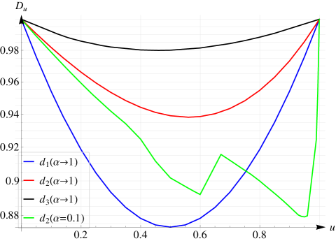
Refer to caption


Figure 7: The u𝑢u-divergence as a function of u𝑢u for the LFDs obtained for various pairs of distributions as well as uncertainty classes.

Refer to caption


Figure 8: KKT parameters for two pairs of nominal distributions and the KL-divergence neighborhood with ϵ0=ϵ1=0.1subscriptitalic-ϵ0subscriptitalic-ϵ10.1\epsilon_{0}=\epsilon_{1}=0.1.

VII-C Asymptotically Minimax Robust NP-tests

Dabak’s test is neither minimax robust nor asymptotically minimax robust as it was shown in Section VVI-A. This result can be demonstrated with an example. Let the nominal distributions be given as in Table I with d2subscript𝑑2d_{2} and let ϵ0=ϵ1=0.01subscriptitalic-ϵ0subscriptitalic-ϵ10.01\epsilon_{0}=\epsilon_{1}=0.01. The rate functions I0subscript𝐼0I_{0} and I1subscript𝐼1I_{1} are of interest for two cases; |a|_{a}^{\cdot} and |a|_{a^{*}}^{\cdot}, i.e. when the test is asymptotically minimax robust Type-I NP-test and Dabak’s test, respectively. Figures 9 and 10 illustrate the rate functions I0subscript𝐼0I_{0} and I1subscript𝐼1I_{1}. Both in Figure 9 and Figure 10 the performance of the (asuperscript𝑎a^{*})-test is degraded by the data samples obtained from the LFDs of the (a)𝑎(a)-test in comparison to those obtained from the LFDs of the (asuperscript𝑎a^{*})-test.

VII-D Band Model

Asymptotically minimax robust tests arising from the band model can similarly be simulated. Consider the lower bounding functions

g0L(y)=(1ϵ)f𝒩(y;1,4),g1L(y)=(1ϵ)f𝒩(y;1,4),formulae-sequencesuperscriptsubscript𝑔0𝐿𝑦1italic-ϵsubscript𝑓𝒩𝑦14superscriptsubscript𝑔1𝐿𝑦1italic-ϵsubscript𝑓𝒩𝑦14g_{0}^{L}(y)=(1-\epsilon)f_{\mathcal{N}}(y;-1,4),\quad g_{1}^{L}(y)=(1-\epsilon)f_{\mathcal{N}}(y;1,4),

where the contamination ratio is chosen to be ϵ=0.2italic-ϵ0.2\epsilon=0.2. Furthermore, let the upper bounding functions be

g0U(y)=(1+ε)f𝒩(y;1,4),g1U(y)=(1+ε)f𝒩(y;1,4),formulae-sequencesuperscriptsubscript𝑔0𝑈𝑦1𝜀subscript𝑓𝒩𝑦14superscriptsubscript𝑔1𝑈𝑦1𝜀subscript𝑓𝒩𝑦14g_{0}^{U}(y)=(1+\varepsilon)f_{\mathcal{N}}(y;-1,4),\quad g_{1}^{U}(y)=(1+\varepsilon)f_{\mathcal{N}}(y;1,4),

with the parameters ε=0.2𝜀0.2\varepsilon=0.2 (Type-I), ε=0.5𝜀0.5\varepsilon=0.5 (Type-II), ε=1.5𝜀1.5\varepsilon=1.5 (Type-III) or ε=19𝜀19\varepsilon=19 (Type-III), simulating three different types of robust LRFs resulting from the band model, cf. Section VI-E.
For this setup, and excluding ε=19𝜀19\varepsilon=19 for the sake of clarity, Figure 11 illustrates the corresponding LFDs together with the lower bounding functions, and the upper bounding functions for ε=1.5𝜀1.5\varepsilon=1.5. For ε=0.5𝜀0.5\varepsilon=0.5, the LFDs are overlapping around y=0𝑦0y=0, leading to l^=1^𝑙1\hat{l}=1. This type of overlapping has previously been reported by [10] for single-sample minimax robust tests obtained from the KL-divergence neighborhood. However, the test in [10] is not minimax robust unless a well defined randomized decision rule is used.
In Figure 12, the corresponding robust likelihood ratio functions are illustrated. Increasing ε𝜀\varepsilon transforms the corresponding robust LRF from Type-I to Type-II and then to Type-III. Further increasing ε𝜀\varepsilon, i.e. when ε=19𝜀19\varepsilon=19, the robust LRF tends to a clipped likelihood ratio test, which is the limiting LRF stated in Section VI-E. The robust LRFs can take different shapes depending on the bounding functions. Similar patterns were stated in [18] and also observed in [19].
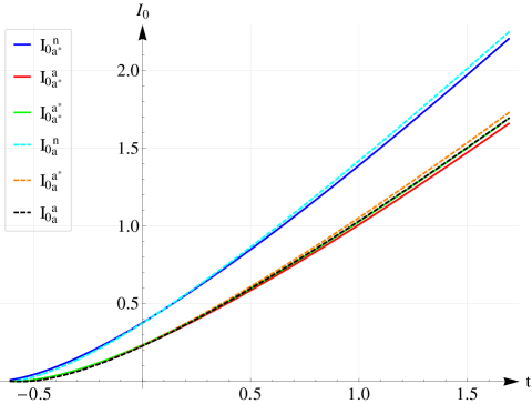
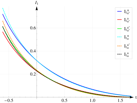
Refer to caption


Figure 9: Asymptotic decay rate of the false alarm probability I0subscript𝐼0I_{0} for the asymptotically minimax robust NP-test ((a)-test) and Dabak’s test ((a)-test).

Refer to caption


Figure 10: Asymptotic decay rate of the miss detection probability I1subscript𝐼1I_{1} for the asymptotically minimax robust NP-test ((a)-test) and Dabak’s test ((a)-test).

Refer to caption


Figure 11: Three different pairs of LFDs arising from the band model together with the bounding functions for ε{0.2,0.5,1.5}𝜀0.20.51.5\varepsilon\in\{0.2,0.5,1.5\}.

Refer to caption


Figure 12: Three different types of Robust LRFs arising from the band model for ε{0.2,0.5,1.5,19}𝜀0.20.51.519\varepsilon\in\{0.2,0.5,1.5,19\} together with the nominal LRF.

VII-E Moment Classes

The LFDs and robust LRFs arising from the moment classes can be exemplified by solving the convex optimization problem given in Section V-C numerically, by first replacing the constraints with the ones defined by the moment classes. Consider the constraints
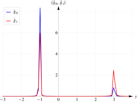
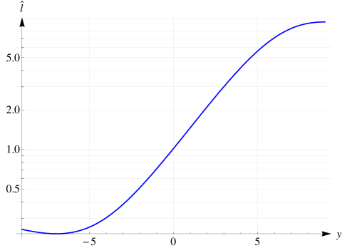
22absent\displaystyle-2\leq 𝔼G0[Y]0.5,subscript𝔼subscript𝐺0delimited-[]𝑌0.5\displaystyle\mathbb{E}_{G_{0}}[Y]\leq-0.5, 0.5𝔼G1[Y]2,0.5subscript𝔼subscript𝐺1delimited-[]𝑌2\displaystyle 0.5\leq\mathbb{E}_{G_{1}}[Y]\leq 2,
00absent\displaystyle 0\leq 𝔼G0[Y2]2,subscript𝔼subscript𝐺0delimited-[]superscript𝑌22\displaystyle\mathbb{E}_{G_{0}}[Y^{2}]\leq 2, 2𝔼G1[Y2]4,2subscript𝔼subscript𝐺1delimited-[]superscript𝑌24\displaystyle 2\leq\mathbb{E}_{G_{1}}[Y^{2}]\leq 4,

Refer to caption


Figure 13: Least favorable distributions arising from the moment classes in the given example.

Refer to caption


Figure 14: The robust LRF arising from the moment classes in the given example.

defined over the first and second moments of the probability density functions. Figures 13 and 14 illustrate the LFDs and the corresponding robust LRF, respectively.
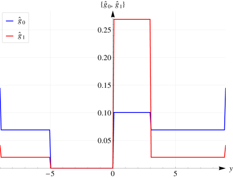
VII-F P-point Classes

Similarly, an example to the asymptotically minimax robust test arising from the p-point classes can be given. Consider the p-point classes defined by the constraints

53g0(y)𝑑y0.3,03g1(y)𝑑y0.8.formulae-sequencesuperscriptsubscript53subscript𝑔0𝑦differential-d𝑦0.3superscriptsubscript03subscript𝑔1𝑦differential-d𝑦0.8\displaystyle\int_{-5}^{3}g_{0}(y)dy\leq 0.3,\quad\int_{0}^{3}g_{1}(y)dy\geq 0.8.

Figures 15 and 16 illustrate the LFDs and the corresponding robust LRF, respectively.
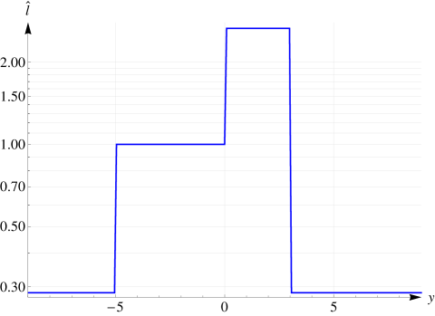
Refer to caption

Figure 15: Least favorable distributions arising from the p-point classes in the given example.

Refer to caption

Figure 16: The robust LRF arising from the p-point classes in the given example.

VIII Conclusions

Designing (asymptotically) minimax robust hypothesis tests for any reasonable construction of uncertainty classes was shown to be made via maximizing Du(G0,G1)subscript𝐷𝑢subscript𝐺0subscript𝐺1D_{u}(G_{0},G_{1}) over all (g0,g1)𝒢0×𝒢1subscript𝑔0subscript𝑔1subscript𝒢0subscript𝒢1(g_{0},g_{1})\in\mathscr{G}_{0}\times\mathscr{G}_{1} and minimizing u𝑢u over all u(0,1)𝑢01u\in(0,1). The uncertainty classes based on the KL-divergence, α𝛼\alpha-divergence, symmetrized α𝛼\alpha-divergence, total variation distance, as well as the band model, moment classes and p-point classes were considered. For the first six classes, the KKT multipliers were employed to derive the LFDs and the corresponding minimax robust tests in parametric forms. The related parameters can be determined by means of solving non-linear systems of equations. For the last two classes, asymptotically minimax robust tests were evaluated as a convex optimization problem.
In addition to the Bayesian formulation, Neyman-Pearson formulations of the asymptotically minimax robust hypothesis testing schemes were considered for the KL-divergence neighborhood. The resulting Neyman-Pearson tests of Type I and II correspond to a non-linear transformation of the nominal LRF, which involves the Lambert-W function. This result proves that Dabak’s test is not asymptotically minimax robust.
Existence of a deterministic single-sample minimax robust test implies existence of all-sample minimax robust tests. It is also known that a single-sample minimax robust test may fail to exist even for a simple example. Besides, randomized versions of single-sample minimax robust tests, if they exist, do not lead to finite-sample minimax robust tests. These results inevitably motivate considering asymptotical designs. Although the term asymptotic implies validity of the theory for very large sample sizes, it was shown that the proposed theory allows finding the finite-sample minimax robust test, if it exists and the asymptotically minimax robust test, otherwise. Therefore, in some sense, the asymptotic design may be called the best possible approach in terms of minimax robustness.
In order to evaluate theoretical findings and their applicability simulations were performed. In particular, the LFDs and the robust LRFs were exemplified for every uncertainty class considered. While clipping the nominal likelihood ratios has already been known to be a way of employing minimax robustness, it was first observed here that asymptotically minimax robustness may require amplifying the nominal likelihood ratios by a great factor. Additionally, a large number of constraints may be required such that the LFDs resulting from the moment and p-point classes are smooth enough. From this work the following questions are open:

  • Is it true that if f0(y)=f1(y)subscript𝑓0𝑦subscript𝑓1𝑦f_{0}(-y)=f_{1}(y) for all y𝑦y, then u=1/2𝑢12u=1/2 is the minimizer for all/some pairs of uncertainty classes?

  • How should the asymptotic design look like if each random variable Yksubscript𝑌𝑘Y_{k} is subjected to different uncertainties, or if Yksubscript𝑌𝑘Y_{k} are not mutually independent?

Appendix A Existence of a Saddle Value for (21)

Theorem A.1 (Application of Sion’s minimax theorem [37]).

A solution to (21) exists if the following conditions hold:

  • The objective function Dusubscript𝐷𝑢D_{u} is real valued, upper semi-continuous and quasi-concave on 𝒢0×𝒢1subscript𝒢0subscript𝒢1{\mathscr{G}}_{0}\times{\mathscr{G}}_{1} for all u[0,1]𝑢01u\in[0,1].

  • The objective function Dusubscript𝐷𝑢D_{u} is lower semi-continuous and quasi-convex on [0,1]01[0,1] for all (G0,G1)𝒢0×𝒢1subscript𝐺0subscript𝐺1subscript𝒢0subscript𝒢1(G_{0},G_{1})\in{\mathscr{G}}_{0}\times{\mathscr{G}}_{1}.

  • [0,1]01[0,1] is a compact convex subset of a linear topological space.

  • 𝒢0×𝒢1subscript𝒢0subscript𝒢1{\mathscr{G}}_{0}\times{\mathscr{G}}_{1} is a convex subset of a linear topological space.

Proof:

The objective function is real valued, continuous in u𝑢u and (g0,g1)subscript𝑔0subscript𝑔1(g_{0},g_{1}), jointly concave on 𝒢0×𝒢1subscript𝒢0subscript𝒢1{\mathscr{G}}_{0}\times{\mathscr{G}}_{1} for all u[0,1]𝑢01u\in[0,1], and convex on [0,1]01[0,1] for all (G0,G1)𝒢0×𝒢1subscript𝐺0subscript𝐺1subscript𝒢0subscript𝒢1(G_{0},G_{1})\in{\mathscr{G}}_{0}\times{\mathscr{G}}_{1}, see 222nd and 333rd properties of Dusubscript𝐷𝑢D_{u}. The set [0,1]01[0,1] is trivially convex and is closed and bounded, hence compact with respect to the standard topology by Heine-Borel theorem [50, Theorem 2.41]. Finally, 𝒢0subscript𝒢0{\mathscr{G}}_{0} and 𝒢1subscript𝒢1{\mathscr{G}}_{1} are convex sets, since Dfsubscript𝐷𝑓D_{f} is a convex distance. As a result 𝒢0×𝒢1subscript𝒢0subscript𝒢1{\mathscr{G}}_{0}\times{\mathscr{G}}_{1} is also convex. ∎

Appendix B Proof of Theorem IV.3

Proof:

For any t𝑡t, for which I1(t)>I0(t)subscript𝐼1𝑡subscript𝐼0𝑡I_{1}(t)>I_{0}(t) we have

PE(n,t)=P0CF(n)exp(nI0(t))asn,subscript𝑃𝐸𝑛𝑡subscript𝑃0subscript𝐶𝐹𝑛𝑛subscript𝐼0𝑡as𝑛P_{E}(n,t)=P_{0}C_{F}(n)\exp(-nI_{0}(t))\,\,\text{as}\,\,n\to\infty, (68)

since

PE(n,t)P0CF(n)exp(nI0(t))subscript𝑃𝐸𝑛𝑡subscript𝑃0subscript𝐶𝐹𝑛𝑛subscript𝐼0𝑡\displaystyle\frac{P_{E}(n,t)}{P_{0}C_{F}(n)\exp(-nI_{0}(t))} =P0CF(n)exp(nI0(t))+(1P0)CM(n)exp(nI1(t))P0CF(n)exp(nI0(t))absentsubscript𝑃0subscript𝐶𝐹𝑛𝑛subscript𝐼0𝑡1subscript𝑃0subscript𝐶𝑀𝑛𝑛subscript𝐼1𝑡subscript𝑃0subscript𝐶𝐹𝑛𝑛subscript𝐼0𝑡\displaystyle=\frac{P_{0}C_{F}(n)\exp(-nI_{0}(t))+(1-P_{0})C_{M}(n)\exp(-nI_{1}(t))}{P_{0}C_{F}(n)\exp(-nI_{0}(t))}
=1+C(n)exp(n(I1(t)I0(t)))1,absent1𝐶𝑛𝑛subscript𝐼1𝑡subscript𝐼0𝑡1\displaystyle=1+C(n)\exp(-n(I_{1}(t)-I_{0}(t)))\to 1, (69)

where

C(n)=(1P0)CM(n)P0CF(n).𝐶𝑛1subscript𝑃0subscript𝐶𝑀𝑛subscript𝑃0subscript𝐶𝐹𝑛C(n)=\frac{(1-P_{0})C_{M}(n)}{P_{0}C_{F}(n)}. (70)

This argument is true because I1(t)I0(t)>0subscript𝐼1𝑡subscript𝐼0𝑡0I_{1}(t)-I_{0}(t)>0 and C(n)𝐶𝑛C(n) is sub-exponential since from (16) we have

1n(log((1P0)CM(n))log(P0CF(n)))=0asn.1𝑛1subscript𝑃0subscript𝐶𝑀𝑛subscript𝑃0subscript𝐶𝐹𝑛0as𝑛\frac{1}{n}(\log((1-P_{0})C_{M}(n))-\log(P_{0}C_{F}(n)))=0\,\,\text{as}\,\,n\to\infty. (71)

Similarly, for the case I1(t)<I0(t)subscript𝐼1𝑡subscript𝐼0𝑡I_{1}(t)<I_{0}(t) we have

PE(n,t)=(1P0)CM(n)exp(nI1(t))asn.subscript𝑃𝐸𝑛𝑡1subscript𝑃0subscript𝐶𝑀𝑛𝑛subscript𝐼1𝑡as𝑛P_{E}(n,t)=(1-P_{0})C_{M}(n)\exp(-nI_{1}(t))\,\,\text{as}\,\,n\to\infty. (72)

Consequently, as n𝑛n\to\infty we have

PE(n,t)={P0CF(n)exp(nI0(t)),I1(t)>I0(t)(1P0)CM(n)exp(nI1(t)),I0(t)>I1(t),subscript𝑃𝐸𝑛𝑡casessubscript𝑃0subscript𝐶𝐹𝑛𝑛subscript𝐼0𝑡subscript𝐼1𝑡subscript𝐼0𝑡1subscript𝑃0subscript𝐶𝑀𝑛𝑛subscript𝐼1𝑡subscript𝐼0𝑡subscript𝐼1𝑡P_{E}(n,t)=\begin{cases}P_{0}C_{F}(n)\exp(-nI_{0}(t)),&I_{1}(t)>I_{0}(t)\\ (1-P_{0})C_{M}(n)\exp(-nI_{1}(t)),&I_{0}(t)>I_{1}(t)\end{cases}, (73)

which can be rewritten as

PE(n,t)=P0a(1P0)1aCF(n)aCM(n)1aexp(nmin{I0(t),I1(t)})subscript𝑃𝐸𝑛𝑡superscriptsubscript𝑃0𝑎superscript1subscript𝑃01𝑎subscript𝐶𝐹superscript𝑛𝑎subscript𝐶𝑀superscript𝑛1𝑎𝑛subscript𝐼0𝑡subscript𝐼1𝑡P_{E}(n,t)=P_{0}^{a}(1-P_{0})^{1-a}C_{F}(n)^{a}C_{M}(n)^{1-a}\exp(-n\min\{I_{0}(t),I_{1}(t)\}) (74)

where a=𝟏{I1>I0}𝑎subscript1subscript𝐼1subscript𝐼0a=\mathbf{1}_{\{I_{1}>I_{0}\}}. Hence, as n𝑛n\to\infty

mintPE(n,t)subscript𝑡subscript𝑃𝐸𝑛𝑡\displaystyle\min_{t}P_{E}(n,t) mintexp(nmin{I0(t),I1(t)})mintnmin{I0(t),I1(t)}absentsubscript𝑡𝑛subscript𝐼0𝑡subscript𝐼1𝑡subscript𝑡𝑛subscript𝐼0𝑡subscript𝐼1𝑡\displaystyle\equiv\min_{t}\exp(-n\min\{I_{0}(t),I_{1}(t)\})\equiv\min_{t}-n\min\{I_{0}(t),I_{1}(t)\}
maxtmin{I0(t),I1(t)}mintmax{I0(t),I1(t)},absentsubscript𝑡subscript𝐼0𝑡subscript𝐼1𝑡subscript𝑡subscript𝐼0𝑡subscript𝐼1𝑡\displaystyle\equiv\max_{t}\min\{I_{0}(t),I_{1}(t)\}\equiv\min_{t}\max\{I_{0}(t),I_{1}(t)\}, (75)

since P0a(1P0)1aCF(n)aCM(n)1asuperscriptsubscript𝑃0𝑎superscript1subscript𝑃01𝑎subscript𝐶𝐹superscript𝑛𝑎subscript𝐶𝑀superscript𝑛1𝑎P_{0}^{a}(1-P_{0})^{1-a}C_{F}(n)^{a}C_{M}(n)^{1-a} is positive and independent of t𝑡t. From [7, Remark. 5.2.2.], I0subscript𝐼0I_{0} and I1subscript𝐼1I_{1} are increasing and decreasing functions of u𝑢u, respectively. Let hj:ut:subscript𝑗maps-to𝑢𝑡h_{j}:u\mapsto t be the mapping between maximizing u𝑢u and t𝑡t in (15). It is easy to see that hjsubscript𝑗h_{j} is increasing because it is the derivative of a convex function logMX1j(u)superscriptsubscript𝑀subscript𝑋1𝑗𝑢\log M_{X_{1}}^{j}(u) [2, p. 77]. Hence, I0(t)=I0(h0(u))subscript𝐼0𝑡subscript𝐼0subscript0𝑢I_{0}(t)=I_{0}(h_{0}(u)) and I1(t)=I1(h1(u))subscript𝐼1𝑡subscript𝐼1subscript1𝑢I_{1}(t)=I_{1}(h_{1}(u)) are also increasing and decreasing functions respectively, as

dI0(h0(u))du𝑑subscript𝐼0subscript0𝑢𝑑𝑢\displaystyle\frac{dI_{0}(h_{0}(u))}{du} =I0(h0(u))h0(u)0,absentsubscriptsuperscript𝐼0subscript0𝑢superscriptsubscript0𝑢0\displaystyle=I^{{}^{\prime}}_{0}(h_{0}(u))h_{0}^{{}^{\prime}}(u)\geq 0,
dI1(h1(u))du𝑑subscript𝐼1subscript1𝑢𝑑𝑢\displaystyle\frac{dI_{1}(h_{1}(u))}{du} =I1(h1(u))h1(u)0.absentsubscriptsuperscript𝐼1subscript1𝑢superscriptsubscript1𝑢0\displaystyle=I^{{}^{\prime}}_{1}(h_{1}(u))h_{1}^{{}^{\prime}}(u)\leq 0.

Since I0subscript𝐼0I_{0} and I1subscript𝐼1I_{1} are also increasing and decreasing functions of t𝑡t, and furthermore, as MX11(u)=MX10(u+1)superscriptsubscript𝑀subscript𝑋11𝑢superscriptsubscript𝑀subscript𝑋10𝑢1M_{X_{1}}^{1}(u)=M_{X_{1}}^{0}(u+1) for Gj:=G^jassignsubscript𝐺𝑗subscript^𝐺𝑗G_{j}:=\hat{G}_{j} together with (15) implies I1(t)=I0(t)tsubscript𝐼1𝑡subscript𝐼0𝑡𝑡I_{1}(t)=I_{0}(t)-t, it is true that I0(0)=I1(0)subscript𝐼00subscript𝐼10I_{0}(0)=I_{1}(0) and together with {t:I1>I0}{t:t<0}conditional-set𝑡subscript𝐼1subscript𝐼0conditional-set𝑡𝑡0\{t:I_{1}>I_{0}\}\equiv\{t:t<0\} and {t:I1<I0}{t:t>0}conditional-set𝑡subscript𝐼1subscript𝐼0conditional-set𝑡𝑡0\{t:I_{1}<I_{0}\}\equiv\{t:t>0\} one can write

Im(t)=min{I0(t),I1(t)}={I0(t),t<0I1(t),t>0I0(0)=I1(0),t=0.subscript𝐼𝑚𝑡subscript𝐼0𝑡subscript𝐼1𝑡casessubscript𝐼0𝑡𝑡0subscript𝐼1𝑡𝑡0subscript𝐼00subscript𝐼10𝑡0I_{m}(t)=\min\{I_{0}(t),I_{1}(t)\}=\begin{cases}I_{0}(t),&t<0\\ I_{1}(t),&t>0\\ I_{0}(0)=I_{1}(0),&t=0\end{cases}. (76)

Hence, we have

argsuptIm(t)=0.subscriptsupremum𝑡subscript𝐼𝑚𝑡0\arg\sup_{t}I_{m}(t)=0. (77)

Notice that we need Gj:=G^jassignsubscript𝐺𝑗subscript^𝐺𝑗G_{j}:=\hat{G}_{j} in Theorem IV.1. Else, (76) and (77) do not necessarily hold. ∎

References

  • [1] S. M. Kay, Fundamentals of Statistical Signal Processing, Volume 2: Detection Theory.   Prentice Hall PTR, jan 1998.
  • [2] B. C. Levy, Principles of Signal Detection and Parameter Estimation, 1st ed.   Springer Publishing Company, Incorporated, 2008.
  • [3] S. Kassam, G. Moustakides, and J. Shin, “Robust detection of known signals in asymmetric noise,” IEEE Transactions on Information Theory, vol. 28, no. 1, pp. 84–91, January 1982.
  • [4] A. El-Sawy and V. VandeLinde, “Robust detection of known signals,” IEEE Transactions on Information Theory, vol. 23, no. 6, pp. 722–727, November 1977.
  • [5] J. D. Gibson and J. L. Melsa, Introduction to nonparametric detection with applications, ser. Mathematics in science and engineering.   New York, San Francisco, London: Academic Press, 1975.
  • [6] P. J. Huber and E. M. Ronchetti, Robust statistics; 2nd ed., ser. Wiley Series in Probability and Statistics.   Hoboken, NJ: Wiley, 2009.
  • [7] G. Gül, Robust and Distributed Hypothesis Testing, ser. Lecture Notes in Electrical Engineering.   Springer, 2017, vol. 414.
  • [8] B. C. Levy, “Robust hypothesis testing with a relative entropy tolerance,” IEEE Transactions on Information Theory, vol. 55, no. 1, pp. 413–421, 2009.
  • [9] G. Gül and A. M. Zoubir, “Robust hypothesis testing with α𝛼\alpha -divergence,” IEEE Transactions on Signal Processing, vol. 64, no. 18, pp. 4737–4750, Sept 2016.
  • [10] G. Gül and A. M. Zoubir, “Minimax robust hypothesis testing,” IEEE Transactions on Information Theory, vol. 63, no. 9, pp. 5572–5587, 2017.
  • [11] P. J. Huber, “A robust version of the probability ratio test,” Ann. Math. Statist., vol. 36, pp. 1753–1758, 1965.
  • [12] P. J. Huber and V. Strassen, “Minimax tests and the Neyman-Pearson lemma for capacities,” Ann. Statistics, vol. 1, pp. 251–263, 1973.
  • [13] A. G. Dabak and D. H. Johnson, “Geometrically based robust detection,” in Proceedings of the Conference on Information Sciences and Systems, Johns Hopkins University, Baltimore, MD, May 1994, pp. 73–77.
  • [14] C. Pandit and S. Meyn, “Worst-case large-deviation asymptotics with application to queueing and information theory,” Stochastic Processes and their Applications, vol. 116, no. 5, pp. 724 – 756, 2006.
  • [15] P. J. Huber and V. Strassen, “Robust confidence limits,” Z. Wahrcheinlichkeitstheorie verw. Gebiete, vol. 10, pp. 269–278, 1968.
  • [16] G. Gül, “Minimax robust decentralized hypothesis testing for parallel sensor networks,” IEEE Transactions on Information Theory, vol. 67, no. 1, pp. 538–548, 2021.
  • [17] K. Vastola and H. Poor, “On the p-point uncertainty class (corresp.),” IEEE Transactions on Information Theory, vol. 30, no. 2, pp. 374–376, March 1984.
  • [18] S. Kassam, “Robust hypothesis testing for bounded classes of probability densities (corresp.),” IEEE Transactions on Information Theory, vol. 27, no. 2, pp. 242–247, March 1981.
  • [19] M. Fauß and A. M. Zoubir, “Old bands, new tracks-revisiting the band model for robust hypothesis testing,” IEEE Transactions on Signal Processing, vol. 64, no. 22, pp. 5875–5886, Nov 2016.
  • [20] R. Martin and S. Schwartz, “Robust detection of a known signal in nearly Gaussian noise,” IEEE Transactions on Information Theory, vol. 17, no. 1, pp. 50–56, Jan 1971.
  • [21] S. Kassam and J. Thomas, “Asymptotically robust detection of a known signal in contaminated non-Gaussian noise,” IEEE Transactions on Information Theory, vol. 22, no. 1, pp. 22–26, January 1976.
  • [22] R. Martin and C. McGath, “Robust detection to stochastic signals (corresp.),” IEEE Transactions on Information Theory, vol. 20, no. 4, pp. 537–541, Jul 1974.
  • [23] J. E. Smith, “Generalized chebychev inequalities: Theory and applications in decision analysis,” Oper. Res., vol. 43, no. 5, pp. 807–825, oct 1995.
  • [24] F. Brichet and A. Simonian, “Conservative Gaussian models applied to measurement-based admission control,” in Quality of Service, 1998. (IWQoS 98) 1998 Sixth International Workshop on, May 1998, pp. 68–71.
  • [25] M. A. Johnson and M. R. Taaffe, “An investigation of phase-distribution moment-matching algorithms for use in queueing models,” Queueing Systems, vol. 8, no. 1, pp. 129–147, Dec 1991.
  • [26] A. El-Sawy and V. VandeLinde, “Robust sequential detection of signals in noise,” IEEE Transactions on Information Theory, vol. 25, no. 3, pp. 346–353, May 1979.
  • [27] D. Sakrison, “The rate of a class of random processes,” IEEE Transactions on Information Theory, vol. 16, no. 1, pp. 10–16, January 1970.
  • [28] L. Cimini and S. Kassam, “Robust and quantized wiener filters for p-point spectral classes,” in 14th Conf. on Inform. Sciences and Systems, Princeton University, Princeton, NJ, 1980, pp. 314–319.
  • [29] A. D. Pambudi, M. Fauß, F. Ahmad, and A. M. Zoubir, “Minimax robust landmine detection using forward-looking ground-penetrating radar,” IEEE Transactions on Geoscience and Remote Sensing, vol. 58, no. 7, pp. 5032–5041, 2020.
  • [30] M. R. Leonard and A. M. Zoubir, “Robust sequential detection in distributed sensor networks,” IEEE Transactions on Signal Processing, vol. 66, no. 21, pp. 5648–5662, 2018.
  • [31] A. Seifert, D. Reinhard, A. M. Zoubir, and M. G. Amin, “A robust and sequential approach for detecting gait asymmetry based on radar micro-doppler signatures,” in 2019 27th European Signal Processing Conference (EUSIPCO), 2019, pp. 1–5.
  • [32] E. Ollila and D. E. Tyler, “Distribution-free detection under complex elliptically symmetric clutter distribution,” in 2012 IEEE 7th Sensor Array and Multichannel Signal Processing Workshop (SAM), 2012, pp. 413–416.
  • [33] A. Kammoun, R. Couillet, F. Pascal, and M. Alouini, “Optimal design of the adaptive normalized matched filter detector using regularized tyler estimators,” IEEE Transactions on Aerospace and Electronic Systems, vol. 54, no. 2, pp. 755–769, 2018.
  • [34] E. Ollila, D. E. Tyler, V. Koivunen, and H. V. Poor, “Complex elliptically symmetric distributions: Survey, new results and applications,” IEEE Transactions on Signal Processing, vol. 60, no. 11, pp. 5597–5625, 2012.
  • [35] A. G. Dabak, “A geometry for detection theory,” Ph.D. dissertation, Rice University, May 1993.
  • [36] H. Chernoff, “A measure of asymptotic efficiency for tests of a hypothesis based on the sums of observations,” Annals of Mathematical Statistics, vol. 23, pp. 409–507, 1952.
  • [37] M. Sion, “On general minimax theorems.” Pacific Journal of Mathematics, vol. 8, no. 1, pp. 171–176, 1958.
  • [38] F. Österreicher and D. Feldman, “Divergenzen von wahrscheinlichkeitsverteilungen — integralgeometrisch betrachtet,” Acta Mathematica Academiae Scientiarum Hungarica, vol. 37, no. 4, pp. 329–337, Dec 1981.
  • [39] F. Osterreicher and I. Vajda, “Statistical information and discrimination,” IEEE Transactions on Information Theory, vol. 39, no. 3, pp. 1036–1039, May 1993.
  • [40] A. Guntuboyina, S. Saha, and G. Schiebinger, “Sharp inequalities for f𝑓f -divergences,” IEEE Transactions on Information Theory, vol. 60, no. 1, pp. 104–121, Jan 2014.
  • [41] H. Cramér, “Sur un nouveau théorème-limite de la théorie des probabilités,” Actualités Scientifiques et Industrielles, no. 736, 1938.
  • [42] T. van Erven and P. Harremos, “Rényi divergence and kullback-leibler divergence,” IEEE Transactions on Information Theory, vol. 60, no. 7, pp. 3797–3820, 2014.
  • [43] H. O, “Ueber einen mittelwertsatz,” Nachrichten von der Königl. Gesellschaft der Wissenschaften und der Georg-Augusts-Universität zu Göttingen, vol. 1889, p. 338–47, 1889.
  • [44] A. Cichocki and S. ichi Amari, “Families of alpha- beta- and gamma- divergences: Flexible and robust measures of similarities,” Entropy, vol. 12, no. 6, pp. 1532–1568, 2010.
  • [45] F. Liese and I. Vajda, “On divergences and informations in statistics and information theory,” IEEE Trans. Information Theory, vol. 52, no. 10, pp. 4394–4412, 2006.
  • [46] D. P. Bertsekas, A. Nedić, and A. Ozdaglar, Convex Analysis and Optimization, ser. Athena Scientific optimization and computation series.   Athena Scientific, 2003.
  • [47] F. Liese and I. Vajda, Convex Statistical Distances.   Teubner, Leipzig, 1987, vol. 130.
  • [48] D. Ralph, “Global convergence of damped newton’s method for nonsmooth equations via the path search,” Math. Oper. Res., vol. 19, no. 2, pp. 352–389, 1994.
  • [49] F. A. Potra and S. J. Wright, “Interior-point methods,” J. Comput. Appl. Math., vol. 124, no. 1-2, pp. 281–302, Dec 2000.
  • [50] W. Rudin, Principles of Mathematical Analysis, ser. International series in pure and applied mathematics.   Paris: McGraw-Hill, 1976.