Massive MIMO for Connectivity with Drones: Case Studies and Future Directions

Abstract

Unmanned aerial vehicles (UAVs), also known as drones, are proliferating. Applications such as surveillance, disaster management, and drone racing place high requirements on the communication with the drones in terms of throughout, reliability and latency. Existing wireless technologies, notably WiFi, that are currently used for drone connectivity are limited to short ranges and low-mobility situations. A new, scalable technology is needed to meet future demands on long connectivity ranges, support for fast-moving drones, and the possibility to simultaneously communicate with entire swarms of drones. Massive multiple-input and multiple-output (MIMO), a main technology component of emerging 5G standards, has the potential to meet these requirements.

I Drone Technology is Proliferating

Traditionally, unmanned aerial vehicles (UAVs) in the form of drones have been predominantly used for military applications such as battlefield and airspace surveillance, and border patrol. More recently, due to technological advancements in battery and control technology, and miniaturization of electronics, the use of drones for civilian applications is exploding. Such applications include traffic and crowd monitoring, wildlife conservation, search-and-rescue operations during natural disasters, inspection of non-reachable areas, and the transportation of goods [1, 2, 3, 4, 5]. Inexpensive lightweight quadcopter drones are widely available and routinely used for aerial photography and drone racing. More applications are likely to emerge [6, 5, 3, 4, 7]. Forecasts show that by 2022, the global market for drone-based business services will be over USD 100 billion per year [8].

Government bodies and standardization organizations across the world have taken initiatives towards spectrum allocation and safe drone operations [9, 7, 10, 11]. For example, in 2014, the United Nations Office for the Coordination of the Humanitarian Affairs (OCHA) released an important policy document on the use of civilian UAVs in humanitarian settings [12]. Several 5G use cases for drones were identified by 3GPP [13, 14, 11]: broadband access to under-developed areas, hotspot coverage during sport events, and rapidly deployable “on-demand” densification. Field trials have been carried out in cellular networks by major telecom companies including AT&T, Qualcomm, Nokia and China Telecom, Ericsson and China Mobile [15, 16, 17, 18]. Intel entered into the UAV market by introducing MODEM for drones [17]. In cellular communications, the uses of drones is twofold. On the one hand, the drones can act as flying base stations (BSs) to provide hot-spot coverage during emergency situations [15]. On the other hand, drones acting as user equipments (UEs) can be served by ground stations (GSs) or existing cellular BSs [19]. In this paper, we focus on applications and use cases in which the drones act as UEs.

The potential of multi-drone networks is particularly significant as many small drones can be deployed in a short time to cover a large geographical area [20, 21, 12, 22, 2, 23, 24, 25, 26]. In many applications, the drones, acting as UEs, would stream high-quality imagery to a GS [27, 22, 20]. As the required throughputs are very high, existing wireless technologies are incapable of providing adequate service. In this article, we make the case that massive multiple-input and multiple-output (MIMO) [28], a main 5G physical-layer technology component, can enable reliable high-rate communication with swarms of drones simultaneously. Note that only the GS would be equipped with a massive MIMO antenna array, and that each drone would have a single antenna, enabling light-weight drones.

II Drone communication requirements and challenges

TABLE I: Communication requirements for drones in different use cases [1, 3].

Use cases	Data type	Data rate per drone	Number of drones	Range	Mobility	Latency
Crowd Surveillance, Event coverage, Environment monitoring	Video	Hundreds of Mbps (uncompressed) Tens of Mbps (compressed)	10 – 100 depending on the size of the area	100 m – 3 km	10 – 20 m/s	10 – 100 ms
Agriculture	Image and video	Tens of Mbps	1 – 100 depending on the size of the area and, image and video resolution	5 m – 3 km	5 – 20 m/s	10 – 100 ms
Disaster management, Search and rescue operation	Video	Hundreds of Mbps (uncompressed) Tens of Mbps (compressed)	10 – 100 depending on the size of the area and, image and video resolution	50 m – several km	0 – 30 m/s	$<$40 ms
Aerial videography	Image and video	Hundreds of Mbps (uncompressed) Tens of Mbps (compressed)	1 – 10	100 m – 3 km	0 – 10 m/s	100 ms
Drone racing	Video	Tens of Mbps (uncompressed)	50 – 100	50 m – 1 km	55 m/s	$<$ 40 ms

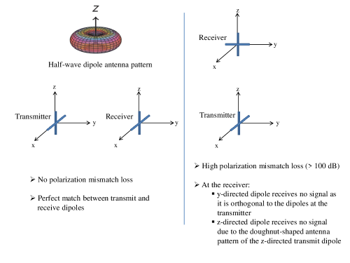
Figure 1: Illustration of polarization loss with different transmit and receive antenna orientations in LoS.

Table I exemplifies the communication requirements of drone networks for various use cases [1, 6, 3]. Some general issues are:

• The channel between the GS and the drones is predominantly line-of-sight (LoS). Since the drones are moving in 3D space, due to flight dynamics (roll, pitch, and yaw rotations), the gains and polarizations of the antennas vary with time. As a result, maintaining connectivity is challenging [29, 30]. Note that polarization mismatch is not a major problem in cellular communications, because due to the large number multi-path components in cellular environments, the probability of having a complete mismatch is negligible as the BSs employ dual-polarized antennas. In contrast, in drone communications, due to the absence of significant multi-path propagation, a drone’s dynamic movement in 3D space can result in very frequent polarization mismatch events. For example, Figure 1 illustrates a setup with a fixed transmit antenna (dual-polarized, half-wave dipole) and two different positions (and orientations) of the receiver antenna (dual-polarized, half-wave dipole). It can be noted that even with dual-polarized antennas the loss can be significant in LoS channel conditions (for more details, see [31]). Therefore, the transmit and the receive antennas must be designed to limit polarization losses.

• The throughput requirements depend on the type of mission, and, for image and video transmission applications, on the capability of the drone’s on-board image processing module. In some cases, it is preferable to transmit raw (uncompressed) video or images. For example, when machine learning is performed in the cloud, large amounts of raw imagery needs be transmitted.

  Throughput requirement in video applications

  Consider a scenario where it is required to scan a $3\times 4$ km area with 20 drones. A 4K (4096 x 2160) resolution video with 60 frames-per-second (FPS) requires a throughput of 64 Mbps per drone, yielding a sum throughput of 1.28 Gbps [31].

  Throughput requirement in image transmissions

  Consider a scenario where a drone has to cover an area of $A_{\mathrm{drone}}$ [m²] with a certain target spatial resolution (see Figure LABEL:GSD_Focal_Length_Illustration). The spatial resolution of the image depends on the ground sampling distance (GSD). The GSD is the distance between the centers of two neighboring pixels measured on the ground, as shown in Figure LABEL:GSD_Focal_Length_Illustration. The area covered by an image, say $A_{\mathrm{image}}$ [m²], depends on the altitude and the properties of the camera, specifically its aspect ratio, focal length, and angle of view (AOV). The flight duration, and the data rate required for transmitting an image with a certain target spatial resolution can be calculated as a function of altitude, GSD, and the properties of the camera (focal length (FL) and pixel size (PS)). The altitude for a given GSD is given by

  $$H=\frac{\mathrm{GSD}\times\mathrm{FL}}{\mathrm{PS}}.$$ (1)

  Let $r_{px}\times r_{py}$ ($r_{px}<r_{py}$) be the camera resolution in pixels. The area covered by an image is $A_{\mathrm{image}}=r_{px}\cdot r_{py}\cdot\mathrm{GSD}^{2}$. Then, for a given AOV, the field of view (FOV) is calculated as

  $$\mathrm{FOV}=2H\tan{\left(\frac{\mathrm{AOV}}{2}\right)}=\mathrm{GSD}\sqrt{r_{px}^{2}+r_{py}^{2}}.$$ (2)

  For example, assume that the target GSD of the mission is 2 cm/pixel, the camera’s AOV is 60 degrees, and $\mathrm{PS}~{}=~{}2.3\times 10^{-6}$ m. When $r_{px}\times r_{py}~{}=~{}$ 2664 $\times$ 1496, we have that the corresponding required $\mathrm{FOV}~{}=~{}$61 m, the required focal length $\mathrm{FL}~{}=~{}2\times~{}10^{-3}$ m, the required drone altitude $H~{}=~{}$53 m, and the resulting area covered by an image $A_{\mathrm{image}}~{}=~{}$1594 m².

  

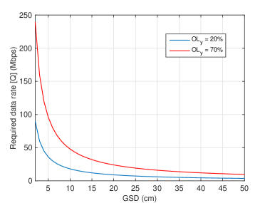
  Figure 3: Required data rate as a function of target GSD with $b~{}=~{}$24 bits/pixel, $\mathrm{CR}~{}=~{}$2:1, and $v~{}=~{}$20 m/s

  Assume that the camera is oriented with the longest edge of the sensor parallel to the flight direction (i.e. $y$-axis as shown in Figure LABEL:drone_image_overlap). Let $b$ be the number of bits per pixel and $\mathrm{CR}$ be the compression ratio. Let $\mathrm{OL}_{y}$ and $\mathrm{OL}_{x}$ be the front and side image overlap (in percent), respectively, required by the mission (see Figure LABEL:drone_image_overlap). Then the number of bits generated by an image is

  $$D_{\mathrm{image}}=\frac{r_{px}\cdot r_{py}\cdot b}{\mathrm{CR}}$$ (3)

  and the time difference between two consecutive image captures is

  $$t=\frac{r_{py}\cdot\mathrm{GSD}\cdot(1-\mathrm{OL}_{y})}{v},$$ (4)

  where $v$ is the drone speed.

  For simplicity, let us assume that $\mathrm{OL}_{x}=$0. Then the instantaneous data rate required by the drone is

  $$Q=\frac{D_{\mathrm{image}}}{t}=\frac{r_{px}\cdot b\cdot v}{\mathrm{GSD}\cdot\mathrm{CR}\cdot(1-\mathrm{OL}_{y})}.$$ (5)

  

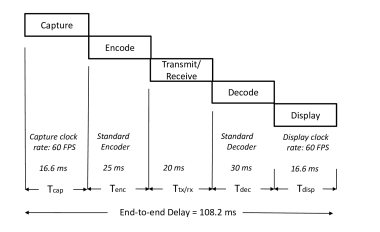
  Figure 4: End-to-end latency in video applications [32].

  Figure 3 shows the required data rate as function of the target GSD with two different values of the image overlap. It can be seen that a higher spatial resolution requires a higher-throughput communication link.

• Connectivity to multiple drones must be ensured simultaneously [20, 21, 12, 22, 2, 23, 24, 25, 26]. This requires either time- or frequency-sharing, which is inefficient. The spatial multiplexing capability of Massive MIMO can be exploited to simultaneously provide high throughput communication links to many drones.

• Reliability and latency are important concerns in many applications. For example, in drone racing, the end-to-end delay should stay below a few tens of milliseconds [33]. If a drone moves at 30 m/s, with a latency of 50 ms, when the pilot sees the video on the display the drone has moved 1.5 meters. Thus, the latency has to be kept as low as possible for drone control and navigation [34, 32]. Figure 4 illustrates the end-to-end latency in video applications. The main components that contribute to the increased latency are video encoding and decoding modules (greater than 50 ms processing time). By transmitting raw video (without any compression) via a high-throughput Massive MIMO based wireless link, it is possible to achieve low-latency in video applications.

• High-mobility support is important [6] as typical flying speeds of drones range from 5 m/s (agricultural crop monitoring, site inspection) to 30 m/s (disaster management).

II-A Inadequacy of existing technologies

Existing wireless technologies such as WiFi and XBee-PRO are unsuitable for drone networks that involve high mobility and a large number of drones. Since these technologies were originally designed for indoor wireless access with very low mobility, they perform poorly in high-mobility conditions [29]. Particularly, due to limitations in the PHY- and MAC-layer protocols, the latency is typically hundreds of milliseconds. Experimental results show that under LoS conditions, the maximum range of WiFi and XBee-PRO is 300–500 m (with 10 Mbps, single drone) and 1 km (with 250 kbps), respectively [21, 35]. Furthermore, more seriously, when multiple drones share resources, due to the limitations of the MAC protocols, the throughput achieved per drone will decrease proportionally [36].

Recently there has been interest in utilizing 4G/5G cellular networks such as LTE for aerial communication [37, 38, 39, 40, 19, 41, 42, 43, 44]. But cellular networks are not suitable for high throughput, long-range aerial communication purposes for the following reasons. Since the BS antennas typically tilted towards ground, measurement results show that, coverage is limited to low altitudes (below 100 m) and low elevation angles [42, 45, 38, 44, 46]. Furthermore, co-channel interference originating from neighboring cells will be a major problem [47, 41]. Since existing cellular BSs are connected to the power grid, they may be unavailable in relevant emergency situations such as earth-quakes or massive flooding. Furthermore, cellular networks are not available in many relevant mountainous and sea environments. In addition, the mobility pattern of drones is different from that of terminals in cellular communications. Pitch, roll and yaw angles of the drones can change rapidly, and may result in poor connectivity due to polarization mismatch.

A new, dedicated technology is required to provide connectivity to drones. A major advantage of developing a new technology for drone networks is that one can design the PHY- and MAC- layer protocols from a clean slate, accounting for the specific requirements of aerial communications.

Figure 5: Allocation of symbols in TDD frame structure

III Massive MIMO is a suitable technology for drone communications

Massive MIMO is a multi-antenna multi-user wireless technology originally developed for cellular communications [28]. The three main features of Massive MIMO are (i) array gain, which translates into a coverage extension; (ii) spatial multiplexing, which permits the service of many tens of terminals in the same time-frequency resource; and (iii) the handling of high mobility through exploitation of channel reciprocity and time-division duplex (TDD) operation [28, 48]. Substantially all signal processing complexity resides at the BS, rendering the terminals low-complexity. Massive MIMO works well both in rich scattering and LoS environments [28, 31, 49]. These features naturally make the technology suitable for drone communications.

While pilot contamination is known to be a limitation in multi-cell massive MIMO systems, for drone communications, due to high coherence bandwidth (assuming the antenna array is directed upwards into the sky) the coherence interval in samples is long and mutually orthogonal pilots to all drones can be afforded. Hence, pilot contamination is not a significant issue, particularly in scenarios where the drone density is low.

Field trials of Massive MIMO in high mobility have been performed for example in the pan-European FP7-MAMMOET project, and efficient hardware implementations have been demonstrated [50, 49]. In terms of digital circuit implementations, zero-forcing precoding and decoding of 8 terminals with 128 BS antennas over a 20 MHz bandwidth can be performed in real time at a power consumption of about 50 milliWatt [51]. Therefore, Massive MIMO GSs for drone communications can be realized at low cost and built from technology that is maturing [52].

In hard-to-reach areas (for example, in mountainous and sea environments) and during natural disaster situations, Massive MIMO-based high-throughput networks can be deployed quickly to cover a large geographical area. A master aircraft equipped with an antenna array can act as a control station to gather information from a swarm of light-weight drones equipped with a single antenna. In urban environments, for providing coverage for high-altitude drones, the antenna array can be placed on top of high-rise buildings. Otherwise, the antenna array can be placed in existing cellular towers, but with appropriate tilting towards the sky.

IV What and how much Massive MIMO can provide for drone communications?

The fundamental principle of Massive MIMO operation is to obtain channel state information (CSI) between the antenna array and all terminals, and then apply appropriate signal processing algorithms. During the uplink training phase, all terminals simultaneously transmit predefined orthogonal pilot sequences to the GS. Upon receiving these pilots, the GS estimates the channels between the GS array and the terminals. TDD operation is used, which permits the exploitation of uplink-downlink channel reciprocity, as long as the uplink and downlink transmissions take place within the channel coherence time.

If the maximum drone speed is $v$ m/s, then the corresponding coherence time is

$$T_{c}\approx\frac{c}{2\cdot v\cdot f_{c}}\ \ \ \text{(s)},$$ (6)

where $f_{c}$ is the carrier frequency and $c$ is the speed of light. With a coherence bandwidth of $B_{c}$ (Hz), the number of samples per coherence interval is

$$\tau=B_{c}T_{c}.$$ (7)

For example, a coherence bandwidth of 3 MHz, a drone speed of 30 m/s, and a carrier frequency of 2.4 GHz, yield $\tau~{}=$ 6250 samples.

Figure 6: Canonical geometric model. The elevation and azimuth angles determine the channel responses of the drones

TDD frame structure: Figure 5 illustrates the TDD-based frame structure where $\tau_{\mathrm{ctrl}}$, $\tau_{\mathrm{ul,p}}$, $\tau_{\mathrm{ul,d}}$, $\tau_{\mathrm{dl,p}}$, and $\tau_{\mathrm{dl,d}}$ denote the number of symbols used for control channel information, uplink pilot transmission, uplink data transmission, downlink pilot transmission, and downlink data transmission, respectively, and $\tau=\tau_{\mathrm{ctrl}}+\tau_{\mathrm{dl,p}}+\tau_{\mathrm{dl,d}}+\tau_{\mathrm{ul,p}}+\tau_{\mathrm{ul,d}}$.

Control information: The command and control information from the GS is transmitted through downlink control channels. The control information consists of important and critical data such as synchronization, scheduling information, and direction or trajectory control [53, 54]. With Massive MIMO, further functionalities can be added, for example: control signals for re-orienting drone’s antenna towards the GS and selection of antenna polarization. In order to achieve high reliability, instead of spatial multiplexing, it is preferred to transmit the control information on orthogonal resource elements [54].

Uplink pilot transmission: If there are $K$ drones in the system, then the number of symbols used for uplink pilot transmission should be greater than or equal to $K$ [28]. The pilot power of the drones is chosen based on the maximum possible distance and the worst-case combined effect of antenna gain and polarization mismatch factor (averaged over all antenna elements), so that a pre-determined received pilot signal-to-noise ratio (SNR) is maintained at the GS. Polarization mismatch losses, per antenna, can be severe in some cases. However, the overall loss can be made small by an appropriate choice of polarization and orientation of the GS array elements.

Uplink data transmission: During uplink data transmission, all drones apply channel inversion power control in order to maintain a pre-determined target data SNR at the GS (averaged over all GS antenna elements).

Downlink pilot transmission: Through broadcasting of (non-directional) pilots by the GS, the drones can measure their path loss. Note that one downlink pilot is sufficient in the downlink training phase.

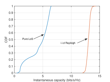
Figure 7: CDF of instantaneous uplink capacity with pure LoS and i.i.d. Rayleigh fading channels with $M=$100 antennas and $K=$20 terminals at 2.4 GHz carrier frequency. The terminal positions are assumed to be uniformly and independently distributed within a sphere of radius 500 m. Uplink channel inversion power control is applied to achieve equal SNR (0 dB) for all terminals.

For the examples presented next, we assume that the GS comprises a uniform linear or rectangular array with $M$ antennas. The drones, in contrast, are equipped with a single antenna. The GS uses fully digital maximum-ratio combining (MRC) processing to decode the data transmitted by the drones.

For given channel vectors of $K$ drones, the instantaneous uplink capacity achieved by the $k$-th drone is given by

$$S_{k}=\log_{2}\left(1+\frac{p_{uk}\left\lVert\boldsymbol{g}_{k}\right\rVert^{4}}{\sum_{j=1,j\neq k}^{K}p_{uj}|\boldsymbol{g}_{k}^{H}\boldsymbol{g}_{j}|^{2}+\left\lVert\boldsymbol{g}_{k}\right\rVert^{2}}\right),$$ (8)

where the $k$-th drone’s channel vector $\boldsymbol{g}_{k}=[g_{k1}\ g_{k2}\ ...\ g_{kM}]^{T}$ and $p_{uj}$ is the transmit power (normalized by the receiver noise power) of $j$-th drone. We consider that there is LoS propagation (no multipath) between the GS antenna array and the drones. The channel between the $l$-th GS antenna and the $k$-th drone’s antenna is given by

$$g_{kl}=\sqrt{\beta_{k}\chi_{kl}}\exp{\left(-\frac{i2\pi\left(d_{k}+(l-1)\delta\sin\theta_{k}\cos\phi_{k}\right)}{\lambda}\right)},$$ (9)

where $\beta_{k}$ represents free-space path loss, $\chi_{kl}$ represents polarization mismatch loss and antenna gain, $d_{k}$ is the distance between the first GS antenna and the drone (see Figure 6), $\delta$ is the antenna element spacing, and $\lambda$ is the operating wavelength.

In practice, the Massive MIMO system performance will lie between pure LoS and rich scattering (i.e., i.i.d. Rayleigh fading) environments. In rich scattering, which is typical of a cellular environment, the channel coefficients are given by

$$g_{kl}\sim\mathcal{CN}(0,\beta_{k}),\ \ l=1,2,...M.$$ (10)

Favorable channel conditions hold with high probability in rich scattering, where channels become asymptotically orthogonal as the number of antennas grows. Interestingly, favorable channel condition can be achieved with large numbers of antennas even in pure LoS scenarios as well [28, Chap. 7]. Figure 7 shows the CDF of the instantaneous capacity achieved by the terminals with two different channel models as given in (9) and (10). With pure LoS, since the channel vectors of different terminals are highly correlated, the capacity of the LoS channel is significantly lower than that of the i.i.d. Rayleigh fading channel. The practical air-to-ground channels are characterized by a small number of multi-path components which is close to the pure LoS channel [55, 56]. Thus, the LoS assumption considered in this paper provides worst-case system design for Massive MIMO based drone communication system.

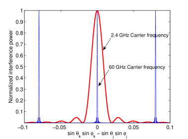
Figure 8: Interference as function of angular separation, quantified in terms of $\sin\theta_{k}\sin\phi_{k}-\sin\theta_{j}\sin\phi_{j}$ with 100 GS antennas. The aperture length is 6.25 m, the same for both carriers (2.4 and 60 GHz). The spacing between the elements is half a wavelength for 2.4 GHz and 12.5 wavelengths at 60 GHz. At 60 GHz, the mainlobe is 25 times narrower than at 2.4 GHz. Note that the actual range of this quantity is between -2 to 2 but for clarity, only the range [-0.1,0.1] is shown.

We use the ergodic rate as performance metric, that is, averaging the instantaneous throughput over all possible drone positions. The justification is that first, owing to the channel-inversion power control, the instantaneous throughput does not depend much on the range, and, second, that the multi-user interference experienced by a drone depends on the relative positions of the other drones and the strength of this interference fluctuates quickly as the drones move. For example, consider the geometric model in Figure 6. The normalized interference power caused by the $j$-th drone towards the $k$-th drone can be expressed as [31]

$$\frac{|\boldsymbol{g}_{k}^{H}\boldsymbol{g}_{j}|^{2}}{\beta_{k}\beta_{j}\chi_{k}\chi_{j}}= \frac{\mathrm{sinc}^{2}\left(M\frac{\delta}{\lambda}(\sin{\theta_{k}}\cos{\phi_{k}}-\sin{\theta_{j}}\cos{\phi_{j}})\right)}{\mathrm{sinc}^{2}\left(\frac{\delta}{\lambda}(\sin{\theta_{k}}\cos{\phi_{k}}-\sin{\theta_{j}}\cos{\phi_{j}})\right)},$$ (11)

where $\mathrm{sinc}(x)=\frac{\sin(\pi x)}{\pi x}$. As an illustration, for the geometric model in Figure 6, Figure 8 shows the strength of the interference that one drone is causing to another, as a function of their angular separation, i.e. $\sin\theta_{k}\sin\phi_{k}-\sin\theta_{j}\sin\phi_{j}$.

Simultaneous high-throughput transmission from a large number of drones

For analytical tractability reasons, assuming that the GS array elements are identically oriented (for the general case, see the next section), for a given distributions of the drones, a lower bound on the uplink ergodic rate (in bits/sec) achieved per drone is given by [31],

$$S=B \left(1-\frac{2\cdot v\cdot f_{c}\left(K+\tau_{\mathrm{dl}}+\tau_{\mathrm{ctrl}}\right)}{B_{c}\cdot c}\right)$$

$$\times\log_{2}\left(1+\frac{M\rho_{u}}{\rho_{u}(K-1)\left(1+\frac{\Omega}{M}\right)+1+\frac{\kappa\ \chi_{wc}}{\rho_{u}\rho_{p}}(1+K\rho_{u})}\right),$$ (12)

where $B$ is the bandwidth and $\tau_{\mathrm{dl}}=\tau_{\mathrm{dl,p}}+\tau_{\mathrm{dl,d}}$ is the number of symbols used for downlink transmission. $\chi_{wc}$ is the lowest possible value of the combined effect of antenna gain and polarization mismatch and $\kappa$ is the average antenna gain and polarization mismatch; $\kappa\ \chi_{wc}<1$.

The quantity $\Omega$ can be interpreted as the correlation between the spatial signatures of two different drones. Consider that the drone positions are distributed uniformly at random within a spherical shell with inner radius $R_{\mathrm{min}}$ and outer radius $R$, where the inner radius is much greater than the array aperture. When the inner radius of the sphere is comparable to the outer radius, the quantity $\Omega$ is given by

$$\Omega=\sum_{l=1}^{M}\sum_{l^{\prime}=1,l^{\prime}\neq l}^{M}\mathrm{sinc}^{2}\left(2(l-l^{\prime})\frac{\delta}{\lambda}\right).$$ (13)

Note that with element spacing equal to an integer multiple of one-half wavelength, the quantity $\Omega$ becomes zero. For any other distributions of the drone positions the rate expression as given in (IV) remains the same except that the quantity $\Omega$ which may be different. Therefore, the expression in (IV) can be used to estimate the throughput performance of practical deployment scenarios.

By virtue of the spatial multiplexing capability of Massive MIMO, many drones can simultaneously transmit high-resolution imagery to the GS. Figure LABEL:Mag_sumThroughput_K exemplifies the sum throughput for different numbers of drones, using a 20 MHz bandwidth and 100 GS antennas. The sum throughput increases up to a certain number of drones and then decreases. This is because the pilot overhead per coherence block is proportional to the number of drones, such that the number of samples available for uplink data transmission decreases with the number of drones. Moreover, it can be observed that the sum throughput is almost the same when the data SNR equals 0 dB and 10 dB. This is so because when increasing the SNR, the sum throughput saturates as the communication becomes interference limited.

Figure 10: Illustration of antenna array with pseudo-randomly oriented elements

Pseudo-randomly oriented circularly polarized antenna elements enable stable link conditions

Coverage in a 3D space requires careful antenna design [29, 6]. The GS array may comprise simple antennas such as cross-dipoles. If all antenna elements are independently oriented in arbitrary directions, then the probability of having a high mismatch loss to all antenna elements can be greatly reduced. Figure LABEL:Magazine_CDF_power shows the cumulative probability distribution of the required transmit power, assuming a noise spectral density of -167 dBm/Hz, and a target SNR of 0 dB. With an available power budget of 100 mW (20 dBm), the probability of coverage is 78% with identically oriented, linearly polarized antennas, but 99.99% with circularly polarized, pseudo-randomly oriented antennas.

The differences in coverage probability stem from signal losses due to polarization mismatches between the GS antennas and the antenna at the drone. By pseudo-randomly orienting the antennas in the GS array as shown in Figure 10, the coverage probability can be greatly improved irrespective of the location and orientation of the drones. To exemplify further, Figures LABEL:Mag_Eff_gain_Cir_I and LABEL:Mag_Eff_gain_Cir_NI show the effective antenna gain for varying azimuth and elevation angles with identically and pseudo-randomly oriented GS array elements, respectively. It can be observed that with identically oriented GS array elements, the effective antenna gain becomes very low (below $-30$ dB) at certain azimuth and elevation angles. Further, the antenna gain varies between -30 dB to 20 dB. On the other hand, with pseudo-randomly oriented GS array elements, the effective antenna gain stays within 10–20 dB.

The array geometry also determines the throughput performance, since it determines the angular resolvability. A rectangular array is preferred over linear and circular arrays due to its 3D resolution and reduced space occupancy. For 2.4 GHz and 60 GHz carrier frequencies, with half-wavelength spacing, the space occupied by a rectangular array with 400 elements is approximately 1.25 m x 1.25 m and 5 cm x 3 cm, respectively.

Moreover, in practice, the choice of element spacing is also important. It is observed that, for uniformly distributed drone positions inside a spherical shell, and MRC signal processing, the throughput is maximized when the GS array elements are spaced at a distance equal to an integer multiple of one-half wavelength [31]. For other distributions of drone positions, the optimal antenna spacing is in general different.

High mobility support

In many environments, the drone speed has only a slight impact on the data rate. For example, in over-water and mountainous settings, with 100 drones, at 2.4 GHz carrier frequency, 3 MHz coherence bandwidth, and if 90% of samples per coherence interval are used for uplink transmission, if we change the drone speed from 0 m/s to 30 m/s, from Eqn. (IV) we can observe that the reduction in throughput is less than 2%. In other environments and at larger carrier frequencies, this loss becomes more significant.

By exploiting the characteristics of LoS propagation, one might reduce the channel estimation overhead. For example, if a drone is moving along a known trajectory as shown in Figure LABEL:drone_image_overlap, the channel will experience a predictable phase shift. Hence, if the channel is known at a specific point in time, it may be predicted during many wavelengths of motion without the transmission of additional pilots. This could further increase the number of samples available for data transmission.

Sub-6 GHz versus mmWave frequencies

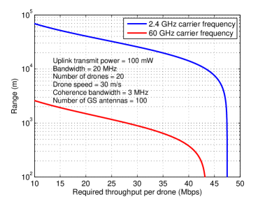
Figure 12: Range vs. required throughput per drone at 2.4 GHz and 60 GHz carrier frequencies. The distribution of the drone positions and the orientation of the GS elements are the same as in Figure LABEL:Mag_sumThroughput_K. Here, for simplicity, the polarization loss is neglected. “Range” refers to the coverage distance of the single antenna system for a given target data SNR.

Massive MIMO can be used for drone communications at both sub-6 GHz and mmWave frequencies. Here we make the following general observations:

• At mmWave frequencies, the energy efficiency is lower, due to decreased effective antenna areas. Suppose that the number of antennas and the target SNRs are fixed. Let $P_{1}$ and $P_{2}$ be the transmit powers required by a drone to maintain a target SNR at a particular distance with carrier frequencies $f_{c1}$ and $f_{c2}$, respectively. From Friis’s free-space equation, assuming unit antenna gains and perfect polarization match, the required transmit powers are related as

  $$P_{2}=P_{1}\left(\frac{f_{c2}}{f_{c1}}\right)^{2}.$$ (14)

  For example, if $f_{c1}=2.4$ GHz and $f_{c2}=60$ GHz, then $P_{2}=625P_{1}$.

• The coverage at mmWave and sub-6 GHz frequencies will be significantly different as the coverage range is inversely proportional to the carrier frequency. From Friis’s transmission formula, assuming unity antenna gains, for a given transmit power of $P_{t}$, bandwidth of $B$ Hz, and a target data SNR of $\rho_{u}$, the range is given by

  $$R=\frac{c}{4\pi f_{c}}\sqrt{\frac{P_{t}}{N_{0}B\rho_{u}}},$$ (15)

  where $N_{0}$ is noise power spectral density in Watts/Hz.

• Figure 12 shows the range supported at 2.4 and 60 GHz carrier frequency, respectively, for different throughput requirements with a 20 MHz bandwidth and a drone transmit power of 20 dBm. The range supported at 2.4 GHz is significantly higher than that at 60 GHz. For example, with a target throughput of 40 Mbps per drone, the supported range is 14 km and 370 m at 2.4 and 60 GHz, respectively. Note that here “range” refers to the coverage distance of the control channels. Since the control channel transmission takes place before and during the CSI acquisition, the range is the same as that of single antenna system and it remains constant irrespective of the number of GS antennas. In contrast, the range of data channels will depend on the number of GS antennas due to the coherent beamforming gain.

  Figure 15: Massive MIMO use cases

• The abundant bandwidth available at mmWave frequencies can be utilized for achieving high sum throughput (in the order of $10$ Gbps). However, due to limitations on the drones’ transmitted power, the coverage range might be limited.

Coverage extension removes the need for multi-hop solutions

Another important feature of Massive MIMO is the coverage extension offered by the coherent beamforming gain. When compared with a single-antenna system, if the GS is equipped with $M$ antennas and under conditions when the GS can obtain accurate channel estimates, the coverage distance of the data channels can be extended by a factor of $\sqrt{M}$. Thus Massive MIMO technology is a promising alternative to multi-hop solutions, which suffer from issues with reliability and latency, and difficulties in coordinating the transmissions [57].

Channel and interference hardening make low latency communication possible

In wireless links, variations in the channel lead to frequent retransmissions. This often results in increased latency. But in Massive MIMO, due to channel hardening, the effective channel gain becomes deterministic (both in LoS and in fading) [28, 58]. In multi-drone networks, similar to channel hardening, interference hardening takes place with large numbers of antennas even in LoS propagation conditions [59]. Therefore, an increased number of antennas at the GS reduces the variations in the SINR. Stable SINR conditions help satisfy low latency requirements.

V Case studies

In this section we detail three different case studies.

V-A Case study I: Emergency response and disaster management

After natural disasters such as earthquakes or massive flooding, drone swarms may be deployed rapidly and help rescue teams to assess the situation in real time (see Figure LABEL:Use-case1). The video received at the GS should have high quality, and in order to obtain high-resolution imagery the drones have to fly at low altitudes. For example, for a given dimension of the camera sensor (resolution ($r_{px}\times r_{py}$): 2664$\times$ 1496, focal length: 5$\times$ 10^-3 m and pixel size: 2.3$\times$ 10^-6 m), for achieving ground sampling distances (GSDs) of 2, 20 cm, and 1 m, from Eqn. (1) we observe that, the required drone altitudes are approximately equal to 44, 435, and 2174 m, respectively.

How many drones required for the mission?

Consider a geographical region to be covered with an area of 4 km $\times$ 4 km, a drone camera resolution of 2664$\times$ 1496, and a required GSD of 20 cm. The area covered by each camera image is 533 m $\times$ 300 m. With a single drone moving at 20 m/s, the total time required to cover the area is more than seven hours. As the flying time of small drones is often limited to 10–30 minutes, a single-drone mission would additionally require a frequent return to base. In contrast, a swarm of drones could cover the area in a short time. For example, to complete the mission in 20 minutes, about 23 drones working in parallel are sufficient.

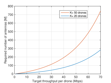
Figure 16: Number of antennas required vs. target throughput per drone at 2.4 GHz carrier frequency for drone speed $v=$ 30 m/s, coherence bandwidth $B_{c}=$ 300 KHz, bandwidth $B=$ 20 MHz and SNR $\rho=$ 0 dB

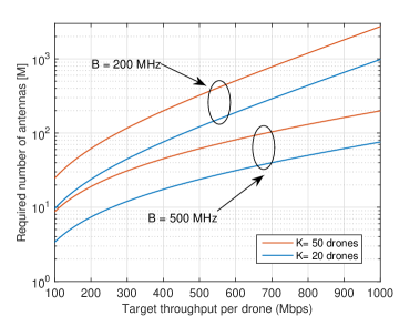
Figure 17: Number of antennas required vs. target throughput per drone at 60 GHz carrier frequency for drone speed $v=$ 20 m/s, coherence bandwidth $B_{c}=$ 3 MHz and SNR $\rho=$ 0 dB

How much data need to be transmitted by a drone?

The uplink (drone to GS) data rate requirement depends on the desired quality of the imagery. JPEG2000 is a loss-less compression standard which gives compression ratios of up to 4:1. H264 and STD are commonly used lossy video compression standards that achieve compression ratios in the range 20:1 to 200:1. For video transmission, the throughput required by a drone is [31]

$$S_{\mathrm{video}}=\frac{r_{px}\cdot r_{py}\cdot b\cdot\mathrm{FPS}}{\mathrm{CR}}\ \text{(bits/sec)},$$ (16)

where $b$ is the number of bits/pixel, $\mathrm{FPS}$ is the number of frames per second, and $\mathrm{CR}$ is the compression ratio. Table II gives the sum throughput requirement with a compression ratio of 200:1 and a GSD of 2 cm. A 4K resolution compressed video requires the sum throughput of 1.46 Gbps. Depending on the environment, more than 200 GS antennas are required to achieve this throughput. The number of required antennas given in Table II is obtained from Eqn. (IV) as

$$M_{\mathrm{req}}= \left((K-1)+\frac{1}{\rho_{u}}+\frac{\kappa\chi_{\mathrm{wc}}}{\rho_{u}^{2}\rho_{p}}(1+K\rho_{u})\right)$$

$$\hskip 28.45274pt\times\left(2^{\frac{Q_{\mathrm{tar}}}{\left(1-\frac{2\cdot v\cdot f_{c}\left(K+\tau_{\mathrm{dl}}\right)}{B_{c}\cdot c}\right)B}}-1\right)$$ (17)

and the range is obtained using (15).

TABLE II: Massive MIMO design parameters for different case studies

Case study	Drone parameters: Number of drones ($K$), Drone speed ($v$), Uplink transmit power ($P_{t}$)	Camera parameters: Pixel resolution (PR), Compression ratio (CR), Framers per second (FPS), Angle of View (AoV), Number of bits per pixel (NBP)	Required uplink sum Throughput ($K\times S$)	Channel parameters: Coherence bandwidth ($B_{c}$), Coherence time ($T_{c}$), Coherence interval ($\tau$)	Massive MIMO design parameters: Carrier frequency ($f_{c}$), Bandwidth ($B$), Number of samples for downlink transmission ($\tau_{\mathrm{dl}}$), Number of antennas ($M$), Data SNR ($\rho_{u}$), Range ($R$)
I. Disaster management	$K=$ 23 $v=$ 20 m/s Altitude = 100 m $P_{t}=$100 mW	PR = 4K CR = 200:1 FPS = 60 NBP = 24	1.39 Gbps	$B_{c}$ = 3 MHz in sea and mountain environments (300 kHz in urban) $T_{c}=3.125$ ms $\tau=9375$ symbols (937 in urban)	$f_{c}=$ 2.4 GHz, $B=$ 20 MHz $\tau_{\mathrm{ul,d}}=\frac{9\tau}{10}$ $M=$ 216 (230 in urban) $\rho_{u}=$ 0 dB $R=$ 5 Km
II. Sport streaming	$K=$ 20 $v=$ 20 m/s $P_{t}=$ 1 W	PR = 4K 360 VR CR = 200:1 FPS = 60 AoV = 90∘ NBP = 24	19.3 Gbps	$B_{c}=$ 3 MHz $T_{c}=$ 0.125 ms $\tau=$ 375 symbols	$f_{c}=$ 60 GHz, $B=$ 300 MHz $\tau_{\mathrm{ul,d}}=\frac{9\tau}{10}$ $M=$ 260 (1035 with $B=$ 200 MHz) $\rho_{u}=$ 0 dB $R=$ 160 m (200 m with $B=$ 200 MHz)
III. Drone racing	$K=25$ $v=30$ m/s $P_{t}=100$ mW	PR = $640\times 480$ CR = $1:1$ FPS = $30$ AoV = $120^{\circ}$ NBP = $8$	1.84 Gbps	$B_{c}=$ 3 MHz $T_{c}=$ 0.862 ms $\tau=$ 2586 symbols	$f_{c}=$ 5.8 GHz, $B=$ 20 MHz $\tau_{\mathrm{ul,d}}=\frac{9\tau}{10}$ $M=$ 420 (840 for $K=$ 50) $\rho_{u}=$ 0 dB $R=$ 2 Km

At 2.4 GHz carrier frequency, Figure 16 illustrates the number of antennas required for a given data rate per drone with 20 and 50 drones. At 60 GHz carrier frequency, Figure 17 shows the number of antennas required for a given data rate per drone with 200 MHz and 500 MHz bandwidths for 20 and 50 drones.

V-B Case study II: Real-time video streaming at sports events

At large-scale sports events, 20 or more quadcopters equipped with 4K (4096 $\times$ 2048) resolution 360-degree cameras can be used to capture the players’ actions at multiple angles (see Figure LABEL:Use-case2) [27]. The captured videos can be sent to an access point equipped with a massive antenna array. This enables real-time virtual reality for the viewers. However, it requires a very high throughput of the wireless link, depending on the desired AoV. For example, using a head-mounted display, with a horizontal AoV of 90 degrees, at any given moment the viewer can see only one-fourth of the scene (or one-third of the scene with a 120-degree AoV).Thus with 4K resolution and 90-degree AoV, each frame will have 16384$\times$ 8192 pixels. With 60 frames per second and 24 bits/pixel, every camera produces approximately 184 Gigabits per second. With a 200:1 compression ratio, the bit rate required by the wireless link is 920 Mbps. If there are 20 drones covering the event, the required sum throughput is 18.4 Gbps.

A typical radius of a large football stadium is approximately 230 m. If we consider that the antenna array is placed on the rooftop of the stadium, the distance between the array and drones will be between 50–100 m. Due to this short range, Massive MIMO technology at mmWave frequencies is a suitable choice. As shown in Table II, at 60 GHz frequency, over 300 MHz bandwidth, with a drone transmit power of 1 W, it is possible to achieve 0 dB SNR at 160 m distance (50 m with 100 mW transmit power). For 20 drones, the number of antennas required to achieve the sum throughput of 18.4 Gbps is 227.

V-C Case study III: Drone Racing

Drone racing, often referred as “the sport of the future,” is attracting big sponsorship deals and venues all over the world [22, 60]. In drone racing contests, see Figure LABEL:Use-case3, pilots wearing goggles control the movement of quadcopters via a First Person View (FPV) interface. The drones can fly at speeds exceeding 100 km/h. Control of the drone movement requires very low latency (tens of milliseconds). Currently, analog transmission is used to reduce the delay between the video capture and display. Due to limited capacity, the maximum number of drones in a race is also limited to 8. Using a massive GS antenna array, hundreds of drones could be simultaneously served on the same time-frequency resource with low latency.

What is the maximum acceptable latency for drone control and video transmission?

For video transmission, latency represents the time difference between the instant a frame is captured by the drone and the instant that frame is shown on the pilot’s display. Including the video capture time, and coding- and decoding delays, the overall end-to-end latency is more than 120 ms [32]. Specifically, standard compression techniques such as H264, STD introduce about 50 ms latency. This delay has serious impact as controlling a drone’s movement in a 3D space requires very low latency. For example, at 40 m/s, a quadcopter moves 2 meters during 50 ms. Adding this lag to the control loop for the pilot makes the flight extra challenging, especially in indoor environments.

The efficiency achieved by standard video compression schemes depends on the differences between subsequent frames. Thus, the successful delivery of a frame depends on the previous frames. As a result, the higher the compression, the greater the possibility of a frame error and frequent retransmissions increase latency. In such situations, one approach to reduce the end-to-end latency is to transmit uncompressed videos by avoiding compression and decompression modules. The end-to-end latency can be made negligible by the use of Massive MIMO enabled high throughput wireless link. To simultaneously support 25 drones in a racing contest, with a moderate video quality, the sum throughput required for transmitting raw video is 1.84 Gbps (with latency less than 70 ms). As shown in Table II about 415 antennas are required to achieve 1.84 Gbps sum throughput.

TABLE III: Air-to-ground channel measurement results

References	Scenario	Altitude	Antenna polarization	Frequency	No. of antennas	Measurement parameters
[61]	Over-sea	370 m - 1.83 km	Vertical	5.7 GHz	1 Tx - 1 Rx	Pathloss & RMS Delay spread
[62]	Over-sea	800 m	Vertical	968 MHz & 5.06 GHz	1 Tx - 1 Rx	Pathloss & RMS Delay spread
[63]	Hilly & Mountain	1 km - 4 km	Vertical	968 MHz & 5.06 GHz	1 Tx - 1 Rx	Pathloss & RMS Delay spread
[64]	Urban	750 m - 1 km	Vertical	968 MHz & 5.06 GHz	1 Tx - 1 Rx	Pathloss & RMS Delay spread
[65]	Desert	900 m - 1 km	Vertical	968 MHz & 5.06 GHz	1 Tx - 1 Rx	Air-frame shadowing loss
[41, 47]	Rural	1.5 m - 120 m	Vertical	800 MHz	1 Tx - 1 Rx	Signal-to-interference ratio
[29]	Outdoor	100 m	Horizontal & Vertical	5 GHz	1 Tx - 1 Rx	Received signal strength
[55]	Urban	450 m - 1 km	Vertical	2 GHz	1 Tx - 4 Rx	RMS Delay spread
[66]	Sub-urban	30 m - 120 m	N/A	700 MHz & 1.9 GHz	N/A	Received signal strength
[38]	Urban	50 m - 300 m	N/A	2.6 GHz	N/A	Latency & Received signal strength
[67]	Urban	50 m - 150 m	N/A	800 MHz	N/A	Received signal strength
[68]	Sub-urban	15 m - 120 m	N/A	800 MHz	N/A	Received signal strength
[6]	Indoor	N/A	Vertical & Circular	5 GHz	N/A	Received signal strength

VI Future Research Directions

A Massive MIMO-enabled drone communication system design involves many challenges. In this section we detail some of the potential research issues that need to be addressed in order to fully exploit the Massive MIMO technology.

Scheduling, resource optimization and 3D trajectory optimization

In practice, there are situations where the channel is changing very slowly (for example, consider two hovering drones at high altitudes with the same azimuth and elevation angles) or the drones positions are closely located [69]. In such conditions the antenna array at the GS might not be able to spatially resolve the channels of the drones and spatial multiplexing becomes impossible; the GS will have to schedule the interfering drones on different time-frequency resources [70]. An alternative approach, if bandwidth is limited and throughput requirements are high, could be to jointly plan the trajectories and the scheduling [19].

New MAC layer design

With Massive MIMO, the frequency of the effective interference variation depends on the GS array geometry, the flying speed and altitude, and range. Furthermore, if the mobility patterns of the drones are known, frequent pilot transmission for CSI estimation is not necessary. Also in many applications, uplink traffic is much higher than the downlink traffic. Thus, a flexible TDD frame structure may be designed taking into account these factors [71, 72].

New flexible MAC layer designs are possible, because unlike existing wireless standards, drone networks do not have backward-compatibility requirements. For video and image transmissions, along with Massive MIMO, efficient cross-layer designs can be utilized to enhance the performance of drone networks [73, 74, 75].

Air-to-ground channel models

The propagation conditions in aerial communications are different from terrestrial land-mobile radio environments. Especially, LoS conditions are generally prevalent with Rician K-factors typically exceeding 25 dB [62, 63, 64, 42, 76]. Table III shows a list of air-to-ground channel measurement results carried out in the recent years. For more detailed survey on air-to-ground channel models, see [77]. The root-mean-square (RMS) delay spread of the channel is an important parameter for Massive MIMO based system design as it determines the coherence interval. For example, measurement results in the C-band (5.03–5.091 GHz), show that the average RMS delay spread is on the order of 10 ns (with an average UAV altitude of 600 m and link ranges from 860 m to several kilometers) in over-water, hilly and mountainous terrain, and 10–60 ns in suburban and near-urban environments [64]. Hence, the coherence bandwidth, if defined as the frequency separation associated with a correlation of 0.5 [78], varies between 3 MHz and 20 MHz.

Although measurement results are unavailable at mmWave frequencies (30 GHz to 300 GHz), due to the reduced number of multipath components, one can expect even higher coherence bandwidths than at sub-6 GHz frequencies.

Currently, the measurement results are available only for linearly polarized (horizontal or vertical) antennas. Moreover, the measurements have been taken without altering the orientation of drone antennas. Measurement campaigns need to be carried out, preferably using circularly polarized antennas, over a wide range of carrier frequencies in various environments such as over-water, mountainous, and urban.

Spectrum management

A drone network’s bandwidth requirement depends on several factors, such as the environment, communication range, density of drones, carrier frequency, duplex mode, power source, and throughput requirements [34, 72]. In applications with low drone densities, the spectrum can be opportunistically shared with existing cellular and satellite communication systems. However, dedicated spectrum may be required in case of control and non- payload communications (CNPC) and applications that involve high drone densities [9]. Furthermore, unlicensed spectrum may be utilized [79]. The spatial multiplexing capabilities of Massive MIMO will be instrumental in reducing the spectrum requirements.

Which duplexing mode: FDD or TDD? TDD is generally more efficient in reciprocity-based MIMO systems [28, 48]. In FDD mode, the number of samples required for CSI acquisition is the limiting factor. The number of uplink pilot symbols per coherence interval is at least equal to the number of drones in TDD. On the other hand, in FDD, it is at least equal to the number of GS antennas plus the number of drones. However, due to the reduced number of multipath components in drone communication scenarios, beam tracking may be feasible, which would reduce the need for CSI acquisition. Detailed analysis is required of different duplexing modes in different environments and applications.

Networking challenges

Future aerial networks will be heterogeneous, and consist of different types of drones: high-altitude and long-endurance UAVs, medium-range UAVs, short-range UAVs, and mini-drones [29, 3, 80, 72]. Nodes in various parts of the network may move at different speeds and have different numbers of antennas. For example, in some applications, at mmWave frequencies, the drones themselves can be equipped with antenna arrays to achieve additional capacity gains [81, 82, 83]. In other applications, the antenna elements may be distributed over a large geographical region [54]. Massive MIMO technology in these cases poses new requirements on synchronization.

Moreover, if transmissions from different GSs are uncoordinated, the SINR may fluctuate unpredictably and create highly non-stationary interference, known as flashlight interference [84]. Suitable interference management techniques are required for efficient operation of Massive MIMO based drone networks with multiple GSs.

VII Summary

Massive MIMO technology is an enabler for wireless connectivity with swarms of drones in applications which require long-range and high-throughput links. This entails equipping the GS with a large antenna array, whereas each drone can have a single antenna. Compelling features of Massive MIMO for this application include: high throughput, spatial multiplexing, coverage extension and high-mobility support. We identified several new and important research problems that are relevant to future Massive MIMO-enabled drone communication networks.

References

- [1] S. Hayat, E. Yanmaz, and R. Muzaffar, “Survey on unmanned aerial vehicle networks for civil applications: A communications viewpoint,” IEEE Communications Surveys Tutorials, vol. 18, no. 4, pp. 2624–2661, Fourth-Quarter 2016.
- [2] L. Gupta, R. Jain, and G. Vaszkun, “Survey of important issues in UAV communication networks,” IEEE Communications Surveys Tutorials, vol. 18, no. 2, pp. 1123–1152, Second-Quarter 2016.
- [3] Y. Zeng, R. Zhang, and T. J. Lim, “Wireless communications with unmanned aerial vehicles: Opportunities and challenges,” IEEE Communications Magazine, vol. 54, no. 5, pp. 36–42, May 2016.
- [4] R. N. Akram, K. Markantonakis, K. Mayes, O. Habachi, D. Sauveron, A. Steyven, and S. Chaumette, “Security, privacy and safety evaluation of dynamic and static fleets of drones,” in Proc. IEEE/AIAA Digital Avionics Systems Conference, Sept. 2017, pp. 1–12.
- [5] M. Mozaffari, W. Saad, M. Bennis, Y. Nam, and M. Debbah, “A tutorial on UAVs for wireless networks: Applications, challenges, and open problems,” CoRR, vol. abs/1803.00680, 2018. [Online]. Available: http://arxiv.org/abs/1803.00680
- [6] M. Asadpour, B. Van den Bergh, D. Giustiniano, K. Hummel, S. Pollin, and B. Plattner, “Micro aerial vehicle networks: An experimental analysis of challenges and opportunities,” IEEE Communications Magazine, vol. 52, no. 7, pp. 141–149, July 2014.
- [7] “Spectrum policy challenges of UAV/Drones,” https://insight.ieeeusa.org/articles/spectrum-policy-challenges-of-uavdrones/, [Online], Accessed: .
- [8] “Drones,” https://www.goldmansachs.com/insights/technology-driving-innovation/drones/, [Online], Accessed: .
- [9] R. J. Kerczewski, J. D. Wilson, and W. D. Bishop, “Frequency spectrum for integration of unmanned aircraft,” in Proc. IEEE/AIAA Digital Avionics Systems Conference (DASC), Oct. 2013, pp. 6D5–1–6D5–9.
- [10] “Civil drones (unmanned aircraft),” https://www.easa.europa.eu/easa-and-you/civil-drones-rpas, [Online], Accessed: .
- [11] 3GPP, “Enhanced LTE support for aerial vehicles (3GPP TR 36.777),” ftp://www.3gpp.org/specs/archive/36_series/36.777, [Online], Accessed: .
- [12] “Unmanned Aerial Vehicles in Humanitarian Response,” https://docs.unocha.org/sites/dms/Documents/Unmanned%20Aerial%20Vehicles%20in%20Humanitarian%20Response%20OCHA%20July%202014.pdf, [Online], Accessed: .
- [13] Qualcomm, “SMARTER: Use case for local UAV collaboration,” http://www.3gpp.org/ftp/tsg_sa/WG1_Serv/TSGS1_71_Belgrade/Docs/S1-152278.zip, [Online], Accessed: .
- [14] “Updated scenarios, requirements and KPIs for 5G mobile and wireless system with recommendations for future investigations,” https://www.metis2020.com/wp-content/uploads/deliverables/METISD1.5v1.pdf, [Online], Accessed: .
- [15] AT&T, “Flying COW connects Puerto Rico,” http://about.att.com/inside_connections_blog/flying_cow_puertori, [Online], Accessed: .
- [16] X. Lin, V. Yajnanarayana, S. D. Muruganathan, S. Gao, H. Asplund, H. Maattanen, M. Bergstrom, S. Euler, and Y. . E. Wang, “The sky is not the limit: LTE for unmanned aerial vehicles,” IEEE Communications Magazine, vol. 56, no. 4, pp. 204–210, Apr. 2018.
- [17] “Aerial technology overview,” https://www.intel.co.uk/content/www/uk/en/technology-innovation/aerial-technology-overview.html, [Online], Accessed: .
- [18] Ericsson, “Drones and networks: Ensuring safe and secure operations,” https://www.ericsson.com/assets/local/publications/white-papers/10201110_wp_dronesandmobilenetworks_nov18.pdf, [Online], Accessed: .
- [19] E. Bulut and I. Guevenc, “Trajectory optimization for cellular-connected UAVs with disconnectivity constraint,” in Proc. IEEE International Conference on Communications Workshops, May 2018, pp. 1–6.
- [20] P. Olsson, J. Kvarnstrom, P. Doherty, O. Burdakov, and K. Holmberg, “Generating UAV communication networks for monitoring and surveillance,” in Proc. International Conference on Control Automation Robotics Vision (ICARCV), Dec. 2010, pp. 1070–1077.
- [21] T. Andre, K. Hummel, A. Schoellig, E. Yanmaz, M. Asadpour, C. Bettstetter, P. Grippa, H. Hellwagner, S. Sand, and S. Zhang, “Application-driven design of aerial communication networks,” IEEE Communications Magazine, vol. 52, no. 5, pp. 129–137, May 2014.
- [22] R. Northfield, “Indoor drone racing flies into London,” Engineering Technology, vol. 10, no. 11, pp. 12–13, Dec. 2015.
- [23] J. A. Kakar, “UAV communications: Spectral requirements, MAV and SUAV channel modeling, OFDM waveform parameters, performance and spectrum management,” https://vtechworks.lib.vt.edu/bitstream/handle/10919/53512/Kakar_JA_T_2015.pdf, [Online], Accessed: .
- [24] I. Mademlis, V. Mygdalis, N. Nikolaidis, M. Montagnuolo, F. Negro, A. Messina, and I. Pitas, “High-level multiple-UAV cinematography tools for covering outdoor events,” IEEE Transactions on Broadcasting, pp. 1–9, 2019.
- [25] M. Campion, P. Ranganathan, and S. Faruque, “A review and future directions of UAV swarm communication architectures,” in Proc. IEEE International Conference on Electro/Information Technology (EIT), May 2018, pp. 0903–0908.
- [26] D. Wu, D. I. Arkhipov, M. Kim, C. L. Talcott, A. C. Regan, J. A. McCann, and N. Venkatasubramanian, “ADDSEN: Adaptive data processing and dissemination for drone swarms in urban sensing,” IEEE Transactions Computers, vol. 66, no. 2, pp. 183 – 198, Feb. 2017.
- [27] X. Wang, A. Chowdhery, and M. Chiang, “Networked drone cameras for sports streaming,” in Proc. IEEE International Conference on Distributed Computing Systems (ICDCS), June 2017, pp. 308–318.
- [28] T. L. Marzetta, E. G. Larsson, H. Yang, and H. Q. Ngo, Fundamentals of Massive MIMO. Cambridge University Press, 2016.
- [29] E. Yanmaz, R. Kuschnig, and C. Bettstetter, “Achieving air-ground communications in 802.11 networks with three-dimensional aerial mobility,” in Proc. IEEE INFOCOM, Apr. 2013, pp. 120–124.
- [30] J. Chen, D. Raye, W. Khawaja, P. Sinha, and I. Guvenc, “Impact of 3D antenna radiation pattern on air-to-ground drone connectivity,” in Proc. IEEE Vehic. Technol. Conf. (VTC), Aug. 2018, pp. 1–5.
- [31] P. Chandhar, D. Danev, and E. G. Larsson, “Massive MIMO for communications with drone swarms,” IEEE Transactions on Wireless Communications, vol. 17, no. 3, pp. 1604–1629, Mar. 2018.
- [32] “Low-latency design considerations for video-enabled drones,” http://www.ti.com/lit/wp/spry301/spry301.pdf, [Online], Accessed: .
- [33] D. Schneider, “Wi-Fi + HD video + drones = still wobbly,” IEEE Spectrum, vol. 54, no. 9, pp. 19–20, Sept. 2017.
- [34] J. Kakar and V. Marojevic, “Waveform and spectrum management for unmanned aerial systems beyond 2025,” in Proc. IEEE International Symposium on Personal, Indoor and Mobile Radio Communications (PIMRC), Oct. 2017, pp. 1–5.
- [35] S. Hayat, E. Yanmaz, and C. Bettstetter, “Experimental analysis of multipoint-to-point UAV communications with IEEE 802.11n and 802.11ac,” in Proc. IEEE International Symposium on Personal, Indoor, and Mobile Radio Communications (PIMRC), Aug. 2015, pp. 1991–1996.
- [36] H. Wu, Y. Peng, K. Long, and S. Cheng, “Performance of reliable transport protocol over IEEE 802.11 wireless LAN: analysis and enhancement,” in Proc. Annual Joint Conference of the IEEE Computer and Communications Societies, June 2002, pp. 599–607.
- [37] I. Bor-Yaliniz and H. Yanikomeroglu, “Is 5g ready for drones?: A look into contemporary and prospective wireless networks from a standardization perspective,” IEEE Wireless Communications Magazine, vol. To Appear, pp. 48–55, Nov. 2019.
- [38] G. Yang, X. Lin, Y. Li, H. Cui, M. Xu, D. Wu, H. Ryden, and S. B. Redhwan, “A telecom perspective on the internet of drones: From LTE-Advanced to 5G,” CoRR, vol. abs/1803.11048, 2018. [Online]. Available: http://arxiv.org/abs/1803.11048
- [39] B. V. D. Bergh, A. Chiumento, and S. Pollin, “LTE in the sky: Trading off propagation benefits with interference costs for aerial nodes,” IEEE Communications Magazine, vol. 54, no. 5, pp. 44–50, May 2016.
- [40] H. C. Nguyen, A. Amorim, J. Wigars, I. Z. Kovacs, T. B. Sørensen, and P. E. Mogensen, “How to ensure reliable connectivity for aerial vehicles over cellular networks,” IEEE Access, vol. 5, pp. 12 304–12 317, Feb. 2018.
- [41] I. Kovacs, R. Amorim, H. C. Nguyen, J. Wigard, and P. Mogensen, “Interference analysis for UAV connectivity over LTE using aerial radio measurements,” in Proc. IEEE Vehicular Technology Conference (VTC-Fall), Sept. 2017, pp. 1–6.
- [42] R. Amorim, H. Nguyen, P. Mogensen, I. Z. Kovács, J. Wigard, and T. B. Sørensen, “Radio channel modeling for UAV communication over cellular networks,” IEEE Wireless Communications Letters, vol. 6, no. 4, pp. 514–517, Aug. 2017.
- [43] G. Geraci, A. Garcia-Rodriguez, L. G. Giordano, D. López-Pérez, and E. Björnson, “Understanding UAV cellular communications: From existing networks to Massive MIMO,” IEEE Access, vol. 6, pp. 67 853–67 865, 2018.
- [44] Y. Zeng, J. Lyu, and R. Zhang, “Cellular-connected UAV: Potential, challenges and promising technologies,” IEEE Wireless Communications, pp. 1–8, 2018.
- [45] G. Geraci, A. Garcia-Rodriguez, L. G. Giordano, D. Lopez-Perez, and E. Bjoernson, “Supporting UAV cellular communications through Massive MIMO,” in Proc. IEEE International Conference on Communications Workshops, May 2018, pp. 1–6.
- [46] B. Galkin, J. Kibilda, and L. A. DaSilva, “Coverage analysis for low-altitude UAV networks in urban environments,” in Proc. IEEE Global Communications Conference, Dec. 2017, pp. 1–6.
- [47] R. Amorim, H. Nguyen, J. Wigard, I. Z. Kovács, T. B. Sørensen, D. Z. Biro, M. Sørensen, and P. Mogensen, “Measured uplink interference caused by aerial vehicles in LTE cellular networks,” IEEE Wireless Communications Letters, vol. 7, no. 6, pp. 958–961, Dec. 2018.
- [48] J. Vieira, F. Rusek, O. Edfors, S. Malkowsky, L. Liu, and F. Tufvesson, “Reciprocity calibration for massive MIMO: Proposal, modeling, and validation,” IEEE Transactions on Wireless Communications, vol. 16, no. 5, pp. 3042–3056, May 2017.
- [49] P. Harris, S. Malkowsky, J. Vieira, E. Bengtsson, F. Tufvesson, W. B. Hasan, L. Liu, M. Beach, S. Armour, and O. Edfors, “Performance characterization of a real-time massive MIMO system with LOS mobile channels,” IEEE Journal on Selected Areas in Communications, vol. 35, no. 6, pp. 1244–1253, June 2017.
- [50] P. Harris, S. Zang, A. Nix, M. Beach, S. Armour, and A. Doufexi, “A distributed Massive MIMO testbed to assess real-world performance and feasibility,” in Proc. IEEE Vehicular Technology Conference (VTC Spring), May 2015, pp. 1–2.
- [51] H. Prabhu, J. N. Rodrigues, L. Liu, and O. Edfors, “3.6 a 60pj/b 300Mb/s 128 x 8 Massive MIMO precoder-detector in 28nm FD-SOI,” in Proc. IEEE International Solid-State Circuits Conference (ISSCC), Feb. 2017, pp. 60–61.
- [52] L. V. der Perre, L. Liu, and E. G. Larsson, “Efficient DSP and circuit architectures for Massive MIMO: State of the art and future directions,” IEEE Transactions on Signal Processing, vol. 66, no. 18, pp. 4717–4736, Setp. 2018.
- [53] NASA, “Control and non-payload communications links for integrated unmanned aircraft operations,” https://ntrs.nasa.gov/archive/nasa/casi.ntrs.nasa.gov/20120016398.pdf, [Online], Accessed: .
- [54] C. She, C. Liu, T. Q. S. Quek, C. Yang, and Y. Li, “Ultra-reliable and low-latency communications in unmanned aerial vehicle communication systems,” IEEE Transactions on Communications, pp. 1–1, 2019.
- [55] W. G. Newhall, R. Mostafa, C. Dietrich, C. R. Anderson, K. Dietze, G. Joshi, and J. H. Reed, “Wideband air-to-ground radio channel measurements using an antenna array at 2 GHz for low-altitude operations,” in IEEE Military Communications Conference (MILCOM), vol. 2, Oct. 2003, pp. 1422–1427 Vol.2.
- [56] R. Rajashekar, M. Di Renzo, K. V. S. Hari, and L. Hanzo, “A beamforming-aided full-diversity scheme for low-altitude air-to-ground communication systems operating with limited feedback,” IEEE Transactions on Communications, vol. 66, no. 12, pp. 6602–6613, Dec. 2018.
- [57] L. R. Pinto, L. Almeida, and A. Rowe, “Demo abstract: Video streaming in multi-hop aerial networks,” in Proc. ACM/IEEE International Conference on Information Processing in Sensor Networks, Apr. 2017, pp. 283–284.
- [58] T. L. Narasimhan and A. Chockalingam, “Channel hardening-exploiting message passing (CHEMP) receiver in large-scale MIMO systems,” IEEE Journal of Selected Topics in Signal Processing, vol. 8, no. 5, pp. 847–860, Oct. 2014.
- [59] P. Chandhar, D. Danev, and E. G. Larsson, “On the outage capacity in Massive MIMO with line-of-sight,” in Proc. IEEE International Workshop on Signal Processing Advances in Wireless Communications (SPAWC), July 2017, pp. 1–6.
- [60] D. Schneider, “Is U.S. drone racing legal? Maaaaybe,” IEEE Spectrum, vol. 52, no. 11, pp. 19–20, Nov. 2015.
- [61] Y. S. Meng and Y. H. Lee, “Measurements and characterizations of air-to-ground channel over sea surface at C-band with low airborne altitudes,” IEEE Transactions on Vehicular Technology, vol. 60, no. 4, pp. 1943–1948, May 2011.
- [62] D. W. Matolak and R. Sun, “Air-ground channel characterization for unmanned aircraft systems–Part I: Methods, measurements, and models for over-water settings,” IEEE Transactions on Vehicular Technology, vol. 66, no. 1, pp. 26–44, Jan. 2017.
- [63] R. Sun and D. W. Matolak, “Air-ground channel characterization for unmanned aircraft systems–Part II: Hilly and mountainous settings,” IEEE Transactions on Vehicular Technology, vol. 66, no. 3, pp. 1913–1925, Mar. 2017.
- [64] D. W. Matolak and R. Sun, “Air-ground channel characterization for unmanned aircraft systems–Part III: The suburban and near-urban environments,” IEEE Transactions on Vehicular Technology, vol. 66, no. 8, pp. 6607–6618, Aug. 2017.
- [65] R. Sun, D. W. Matolak, and W. Rayess, “Air-ground channel characterization for unmanned aircraft systems–Part IV: Airframe shadowing,” IEEE Transactions on Vehicular Technology, vol. PP, no. 99, pp. 1–1, 2017.
- [66] Qualcomm, “LTE unmanned aircraft systems - Trial report,” https://www.qualcomm.com/media/documents/files/lte-unmanned-aircraft-systems-trial-report.pdf, [Online], Accessed: .
- [67] X. Lin, R. Wiren, S. Euler, A. Sadam, H. Maattanen, S. D. Muruganathan, S. Gao, Y. E. Wang, J. Kauppi, Z. Zou, and V. Yajnanarayana, “Mobile networks connected drones: Field trials, simulations, and design insights,” CoRR, vol. abs/1801.10508, 2018. [Online]. Available: http://arxiv.org/abs/1801.10508
- [68] A. Al-Hourani and K. Gomez, “Modeling cellular-to-UAV path-loss for suburban environments,” IEEE Wireless Communications Letters, vol. 7, no. 1, pp. 82–85, Feb. 2018.
- [69] A. Kushleyev, D. Mellinger, C. Powers, and V. Kumar, “Towards a swarm of agile micro quadrotors,” Autonomous Robots, vol. 35, no. 4, pp. 287–300, Nov. 2013.
- [70] H. Yang, “User scheduling in Massive MIMO,” in Proc. IEEE International Workshop on Signal Processing Advances in Wireless Communications (SPAWC), June 2018, pp. 1–5.
- [71] K. Pedersen, F. Frederiksen, G. Berardinelli, and P. Mogensen, “A flexible frame structure for 5G wide area,” in Proc. IEEE Vehicular Technology Conference (VTC-Fall), Sept. 2015, pp. 1–5.
- [72] P. Si, F. R. Yu, R. Yang, and Y. Zhang, “Dynamic spectrum management for heterogeneous UAV networks with navigation data assistance,” in IEEE Wireless Communications and Networking Conference (WCNC), Mar. 2015, pp. 1078–1083.
- [73] R. Immich, E. Cerqueira, and M. Curado, “Towards the enhancement of UAV video transmission with motion intensity awareness,” in Proc. IFIP Wireless Days, Nov. 2014, pp. 1–7.
- [74] M. Karzand, D. J. Leith, J. Cloud, and M. Médard, “Design of FEC for low delay in 5G,” IEEE Journal on Selected Areas in Communications, vol. 35, no. 8, pp. 1783–1793, Aug. 2017.
- [75] M. C. Ilter and H. Yanikomeroglu, “Convolutionally coded SNR-Adaptive transmission for low-latency communications,” IEEE Transactions on Vehicular Technology, vol. 67, no. 9, pp. 8964–8968, Sept. 2018.
- [76] A. I. Alshbatat and L. Dong, “Adaptive MAC protocol for UAV communication networks using directional antennas,” in Proc. International Conference on Networking, Sensing and Control (ICNSC), Apr. 2010, pp. 598–603.
- [77] W. Khawaja, I. Guvenc, D. Matolak, U.-C. Fiebig, and N. Schneckenberger, “A survey of air-to-ground propagation channel modeling for unmanned aerial vehicles,” CoRR, vol. abs/1801.01656, 2018. [Online]. Available: https://arxiv.org/abs/1801.01656
- [78] S. Sesia, I. Toufik, and M. Baker, LTE, The UMTS Long Term Evolution: From Theory to Practice. Wiley Publishing, 2009.
- [79] “Drones, UTM and Spectrum – A review,” http://dronealliance.eu/wp-content/uploads/2016/06/Spectrum-Allocation-White-Paper-Drone-Alliance-Europe-fin.pdf, [Online], Accessed: .
- [80] J. Wang, C. Jiang, Z. Han, Y. Ren, R. G. Maunder, and L. Hanzo, “Taking drones to the next level: Cooperative distributed unmanned-aerial-vehicular networks for small and mini drones,” IEEE Vehicular Technology Magazine, vol. 12, no. 3, pp. 73–82, Sept. 2017.
- [81] Z. Guan, N. Cen, T. Melodia, and S. Pudlewski, “Self-organizing flying drones with Massive MIMO networking,” in Proc. Mediterranean Ad Hoc Networking Workshop (Med-Hoc-Net), June 2018, pp. 1–8.
- [82] T. Cuvelier and R. W. Heath, “MmWave MU-MIMO for aerial networks,” in Proc. International Symposium on Wireless Communication Systems (ISWCS), Aug. 2018, pp. 1–6.
- [83] Y. Hu, Y. Hong, and J. Evans, “Modelling interference in high altitude platforms with 3D LoS Massive MIMO,” in Proc. IEEE International Conference on Communications (ICC), May 2016, pp. 1–6.
- [84] T. Ihalainen, Z. L. Pekka Jänis, P. Lunden, M. Moisio, V. Nurmela, M. A. Uusitalo, C. Wijting, and O. N. Yilmaz, “Flexible scalable solutions for dense small cell networks,” in Proc. Wireless World Research Forum, vol. 30, Apr. 2013, pp. 1–4.