Magnetic neutron star cooling and microphysics

Abstract

Aims. We study the relative importance of several recent updates of microphysics input to the neutron star cooling theory and the effects brought about by superstrong magnetic fields of magnetars, including the effects of the Landau quantization in their crusts.

Methods. We use a finite-difference code for simulation of neutron-star thermal evolution on timescales from hours to megayears with an updated microphysics input. The consideration of short timescales ($\lesssim 1$ yr) is made possible by a treatment of the heat-blanketing envelope without the quasistationary approximation inherent to its treatment in traditional neutron-star cooling codes. For the strongly magnetized neutron stars, we take into account the effects of Landau quantization on thermodynamic functions and thermal conductivities. We simulate cooling of ordinary neutron stars and magnetars with non-accreted and accreted crusts and compare the results with observations.

Results. Suppression of radiative and conductive opacities in strongly quantizing magnetic fields and formation of a condensed radiating surface substantially enhance the photon luminosity at early ages, making the life of magnetars brighter but shorter. These effects together with the effect of strong proton superfluidity, which slows down the cooling of kiloyear-aged neutron stars, can explain thermal luminosities of about a half of magnetars without invoking heating mechanisms. Observed thermal luminosities of other magnetars are still higher than theoretical predictions, which implies heating, but the effects of quantizing magnetic fields and baryon superfluidity help to reduce the discrepancy.

1 Introduction

Heat stored in neutron stars after their birth is gradually lost to neutrino emission and surface radiation. The rate of these losses depends on the characteristics of a neutron star: its mass, magnetic field, and composition of heat-blanketing envelopes. Theoretically calculated luminosity of the star as a function of its age (the cooling curve) is sensitive to the details of the theory of matter in extreme conditions: high densities, temperatures, and magnetic fields, not reachable in the terrestrial laboratory. Therefore, a comparison of observed surface luminosity with theoretical predictions can potentially provide information not only on the characteristics of a given star, but also on the poorly known properties of matter in extreme conditions. The theory of neutron star cooling has been developed in many papers, starting from the pioneering works by Chiu & Salpeter (1964) and Tsuruta & Cameron (1966). For a recent review of this theory, see Potekhin et al. (2015).

Thermal or thermal-like radiation has been detected from several classes of neutron stars. Particularly interesting are isolated neutron stars with confirmed thermal emission, whose thermal X-ray spectra are not blended with emission from accreting matter or magnetosphere. A comprehensive list of such objects found before 2014 has been compiled by Viganò et al. (2013). Many neutron stars from this list are satisfactorily explained by the cooling theory (see, e.g., Yakovlev et al. 2008; Viganò et al. 2013, and Sect. 4 below). However, the magnetars, a special class of neutron star with superstrong magnetic fields (see Mereghetti et al. 2015; Turolla et al. 2015; Kaspi & Beloborodov 2017, for recent reviews), are much more luminous than ordinary cooling neutron stars of the same age. For example, at age $t\sim 10$ kyr, typical thermal luminosities are $\sim(10^{31}-10^{33}$) erg s^-1 for ordinary neutron stars and several times ($10^{33}-10^{35}$) erg s^-1 for magnetars. Their high luminosities are believed to be fed by magnetic energy stored in the neutron star (Duncan & Thompson 1992), but the mechanism of the release of this energy is uncertain. Several possible heating mechanisms suggested by different authors have recently been analyzed by Beloborodov & Li (2016).

The characteristic magnetic fields of magnetars, determined from their spindown according to the standard model of a rotating magnetic dipole in vacuum, range from $\sim 10^{13}$ G to $\approx 2\times 10^{15}$ G (Olausen & Kaspi 2014). In addition to the poloidal magnetic field at the surface, the magnetars are believed to have much stronger toroidal magnetic field embedded in deeper layers (Geppert et al. 2006; Pérez-Azorin et al. 2006), which is corroborated by observations of free precession of the magnetars (Makishima et al. 2014, 2016). For a characteristic poloidal component $B_{\mathrm{pol}}$ of a neutron-star magnetic field to be stable, a toroidal component $B_{\mathrm{tor}}$ must be present, such that, by order of magnitude, $B_{\mathrm{pol}}\lesssim B_{\mathrm{tor}}\lesssim 10^{16}\mbox{\leavevmode\nobreak\ G}\,({B_{\mathrm{pol}}/10^{13}\mbox{\leavevmode\nobreak\ G}})^{1/2}$ (Akgün et al. 2013). Moreover, theoretical arguments (e.g., Bonanno et al. 2005), numerical simulations (e.g., Braithwaite 2008; Lasky et al. 2011; Kiuchi et al. 2011; Mösta et al. 2015), and observational evidence (e.g., Tiengo et al. 2014) show that magnetars possess highly tangled, small-scale magnetic fields, which can be several times stronger than their dipole component (see also Mereghetti et al. 2015; Link & van Eysden 2016, and references therein).

In this paper, we analyze the relative importance of different microphysics inputs in cooling of ordinary neutron stars and magnetars. We model both neutron stars with ground-state and accreted envelopes. We study the sensitivity of the cooling to different microphysics ingredients of the theory, including the equation of state (EoS), baryon superfluidity, opacities, and neutrino emission mechanisms, putting emphasis on the role of recent updates of corresponding theoretical models. We demonstrate the importance of the effects of Landau quantization in the crust of the magnetars on the EoS and thermal conductivity tensor, as well as formation of a condensed radiating surface, possibly covered by a dense atmosphere. The latter effects make the heat-blanketing envelope much more transparent than predicted by the classical theory.

The paper is organized as follows. In Sect. 2, we state the main assumptions, recall the basic equations of the cooling theory, and describe our numerical cooling code. In Sect. 3 we briefly recall the essential physics of neutron star cooling and summarize physics input. In Sect. 4, we examine the influence of different physics input ingredients on cooling of nonmagnetized neutron stars, with special attention being paid to several modern microphysics updates. Section 5 is devoted to the cooling of strongly magnetized neutron stars and the role of Landau quantization. Conclusions are summarized in Sect. 6. Appendices A and B specify some details of our treatment of the EoSs of nonmagnetic and strongly magnetized neutron stars.

2 Simulation of thermal evolution

The most massive central part of a neutron star, its core, consists of a uniform mixture of baryons and leptons. The core is surrounded by the crust, where atomic nuclei form a crystalline lattice, and the electrons form almost ideal, strongly degenerate Fermi gas. In an inner part of the crust, the lattice of nuclei is immersed in a liquid of “dripped” (quasi-free) neutrons. The crust is covered by a liquid layer, the ocean, where the lattice is destroyed by thermal fluctuations. As the star cools down, the bottom layers of the ocean freeze into the crust. The ocean, in turn, is usually covered by a gaseous atmosphere, where the spectrum of outgoing thermal radiation is formed.

About a day after the birth of a neutron star, the temperature everywhere in its interior drops below $10^{10}$ K. At this temperature, the chemical potentials of nucleons at densities $\rho\gtrsim 10^{12}$ g cm^-3 and of electrons at $\rho\gtrsim 10^{8}$ g cm^-3 (without the rest energies) are much higher than their kinetic thermal energies. At these conditions, a good approximation is to describe the state of matter as cold nuclear matter in beta equilibrium, resulting in an effectively barotropic EoS. Therefore neutron-star cooling simulations are traditionally performed by treating the internal mechanical structure of the star as decoupled from its thermal structure. The outer boundary condition for simulations of thermal evolution is then provided by a solution of the stationary heat transport equation at $\rho<\rho_{\mathrm{b}}$, where the commonly accepted value $\rho_{\mathrm{b}}=10^{10}$ g cm^-3 (Gudmundsson et al. 1983) is a trade-off between the applicability of a barotropic EoS at $\rho>\rho_{\mathrm{b}}$ and the stationary approximation at $\rho<\rho_{\mathrm{b}}$.

This approach simplifies the cooling simulations, but it does not allow one to trace the rapid processes in the crust, accompanied by sudden heat release, which may result from accretion episodes, starquakes, magnetic reconnection events, and so on, and which are probably common in the magnetars (Mereghetti et al. 2015; Turolla et al. 2015; Kaspi & Beloborodov 2017). In this paper we follow a different approach, which is traditional for the nondegenerate, nonrelativistic stars, and which was extended to the case of general relativity by Richardson et al. (1979).

We assume the mechanical structure to be spherical. Appreciable deviations from the spherical symmetry can be caused by ultra-strong magnetic fields ($B\gtrsim 10^{17}$ G) or by rotation with ultra-short periods (less than a few milliseconds), but we will not consider such extreme cases. We also assume a spherically symmetric thermal structure. This assumption can be violated by local heat releases or by large-scale (e.g., dipolar) strong magnetic fields. For highly tangled small-scale fields, the spherical symmetry is a reasonable first approximation.

In the spherical symmetry, the thermal and mechanical structure are governed by six first-order differential equations for radius $r$, gravitational potential $\Phi$, gravitational mass $M_{r}$ inside a sphere of radius $r$, luminosity $L_{r}$ passing through this sphere, pressure $P$, and temperature $T$ as functions of the baryon number $a$ interior to a given shell (Richardson et al. 1979; cf. Thorne 1977). The time $t$ enters only the equation for $L_{r}$ in the form of the coordinate time derivative of the entropy per baryon.

The mechanical structure of the star is defined by equations

$$\frac{\mathrm{d}r}{\mathrm{d}a} = \frac{1}{4\pi r^{2}\bar{n}}\,\left(1-\frac{2GM_{r}}{rc^{2}}\right)^{1/2},$$ (1)

$$\frac{\mathrm{d}M_{r}}{\mathrm{d}a} = \frac{\rho}{\bar{n}}\,\left(1-\frac{2GM_{r}}{rc^{2}}\right)^{1/2},$$ (2)

$$\frac{\mathrm{d}\Phi}{\mathrm{d}a} = G\,\frac{M_{r}+4\pi r^{3}P/c^{2}}{4\pi r^{4}\bar{n}}\,\left(1-\frac{2GM_{r}}{rc^{2}}\right)^{-1/2},$$ (3)

$$\frac{\mathrm{d}P}{\mathrm{d}a} = -\left(\rho+\frac{P}{c^{2}}\right)\,\frac{\mathrm{d}\Phi}{\mathrm{d}a},$$ (4)

where $\bar{n}$ is the mean number density of baryons, $G$ is the Newtonian constant of gravitation and $c$ is the speed of light in vacuum. These equations are integrated from $r=0$ and $M_{r}=0$ at the center of the star outwards, starting from a predefined central baryon density and keeping $\rho$ and $P$ related to $\bar{n}$ via the EoS, until the outer boundary condition is satisfied (e.g., a predefined mass density at the outer boundary $\rho_{\mathrm{b}}$ is reached). The boundary condition for $\Phi$ is provided by the Schwarzschild metric outside the star,

$$\mathrm{e}^{2{\Phi(R)/c^{2}}}=1-2GM/c^{2}R,$$ (5)

where $R$ and $M=M_{R}$ are the stellar radius and mass. In practice, Eq. (3) is integrated for a shifted potential $\Phi(r)-\Phi(0)$, with the initial value equal to zero at the center of the star, and afterwards the value of the shift $\Phi(0)$ is found from Eq. (5).

The heat flux through a spherical surface is related to gradient of the redshifted temperature $\tilde{T}=\mathrm{e}^{\Phi/c^{2}}T$ by equation

$$L_{r}=-(4\pi r^{2})^{2}\,\bar{n}\,\kappa\,\mathrm{e}^{-{\Phi/c^{2}}}\,\frac{\mathrm{d}\tilde{T}}{\mathrm{d}a},$$ (6)

where $\kappa$ is the thermal conductivity measured in the local. Finally, time-dependence is introduced by equation (Richardson et al. 1979)

$$\frac{\mathrm{d}(L_{r}\mathrm{e}^{2\Phi/c^{2}})}{\mathrm{d}a}=\mathrm{e}^{2\Phi/c^{2}}\left(\mathcal{E}-T\,\mathrm{e}^{-\Phi/c^{2}}\frac{\partial s}{\partial t}\right),$$ (7)

where $\mathcal{E}$ is the net rate of energy generation per baryon and $\partial s/\partial t$ is the coordinate time derivative of the entropy per baryon ($\mathrm{e}^{-\Phi/c^{2}}{\partial s}/{\partial t}$ is the derivative evaluated in the local rest frame of matter). Equation (7) can be combined with Eq. (6) to form

$$\frac{c_{P}}{\bar{n}}\,\mathrm{e}^{\Phi/c^{2}}\,\frac{\partial T}{\partial t}=\frac{\partial}{\partial a}\,K(a)\,\frac{\partial\tilde{T}}{\partial a}+\frac{\tilde{H}-\tilde{Q}}{\bar{n}}.$$ (8)

Here, $c_{P}$ is the heat capacity per unit volume at constant pressure, $\tilde{H}=\mathrm{e}^{2{\Phi/c^{2}}}H$ and $\tilde{Q}=\mathrm{e}^{2{\Phi/c^{2}}}Q$ are redshifted powers of energy sources and sinks, respectively, per unit volume, and

$$K(a)\equiv(4\pi r^{2})^{2}\,\bar{n}\,\kappa\,\mathrm{e}^{\Phi/c^{2}}.$$ (9)

Equation (8) can be written in the form of the usual thermal diffusion equation

$$\frac{c_{P}}{\bar{n}}\,\frac{\partial\tilde{T}}{\partial t}=\frac{\partial}{\partial a}\,K(a)\,\frac{\partial\tilde{T}}{\partial a}+\frac{\tilde{H}-\tilde{Q}}{\bar{n}}+\frac{c_{P}}{\bar{n}}\,\tilde{T}\,\frac{\partial\Phi}{c^{2}\partial t}.$$ (10)

In practice, the last term on the right-hand side is small compared to typical values of the left-hand side. Therefore, in a finite-difference scheme of solution, this term can be treated as an external source, with $\partial\Phi/\partial t$ evaluated from the solution at the preceding time step. The boundary condition to Eq. (10) at the stellar center is $\partial\tilde{T}/\partial a=0$. The outer boundary condition follows from Eq. (6):

$$\left.\frac{\partial\tilde{T}}{\partial a}\right|_{a=a_{\mathrm{b}}}=-\frac{\mathrm{e}^{{\Phi/c^{2}}}\,{L}_{\mathrm{b}}}{(4\pi r^{2})^{2}\bar{n}\kappa},$$ (11)

where ${L}_{\mathrm{b}}$ is the energy flux through the outer boundary $a=a_{\mathrm{b}}$, which is provided by the quasi-stationary thermal structure of a thin envelope outside this boundary. Since we solve the nonstationary problem using the temperature-dependent EoS in the outer crust, the position of the boundary is not restricted by the requirement that the plasma should be degenerate at $\rho_{\mathrm{b}}=\rho(a_{\mathrm{b}})$. Therefore, the thickness of the quasi-stationary envelope can be adapted to an astrophysical problem of interest. In the present work, we choose the mass of the quasi-stationary envelope $\Delta M$ so as to ensure that plasma is fully ionized at $\rho>\rho_{\mathrm{b}}$. At $B=0$, this condition is guaranteed for the mass of an envelope $\Delta M=10^{-12}M_{\odot}$. In the case of strong magnetic fields we find it appropriate to increase the envelope mass to $\Delta M=(10^{-11}-10^{-9})M_{\odot}$, because the Landau quantization suppresses opacities (see Sect. 3.3), which results in quick thermal relaxation of such massive envelopes. We take the partial ionization into account in the outer quasi-stationary boundary layer only. In the deeper layers, where the time-dependent problem is being solved, we use the fully ionized plasma model.

We solve the set of equations (1) – (10) by a finite-difference scheme on a non-uniform, adaptive grid in $a$ and $t$. First, at $t=0$, we define a starting temperature profile (usually constant $\tilde{T}=10^{10}$ K, but we have checked that the start from $\tilde{T}=5\times 10^{10}$ K changes the surface temperature by $<1$% at $t\gtrsim 1$ hr) and solve the set of equations (1) – (4) by the Runge-Kutta method. In order to prevent accuracy loss in the outer crust and ocean, where $a$ is nearly constant as a function of $\rho$, we use the difference $(a_{\mathrm{b}}-a)$ as an independent variable. At each $t=t_{j}$, we introduce a nonuniform grid in this variable and choose a time step $\Delta t_{j}$ so as to ensure smallness of variations of $T$ and $P$ between the neighboring grid points and between the time $t_{j}$ and $t_{j+1}=t_{j}+\Delta t_{j}$. We solve the difference equation, that approximates Eq. (10), by a purely time-implicit energy-conservative scheme (Samarskii 2001, Chapter 8, Eqs. (35), (36), (39)). This scheme would be unconditionally stable if $c_{P}/\bar{n}$, $K(a)$, $(\tilde{H}-\tilde{Q})/\bar{n}$ were constant, so the time step $\Delta t_{j}$ is not limited by the Courant-Friedrichs-Lewy condition. The values of the coefficients are evaluated at the next layer $t_{j+1}$, so the scheme is nonlinear. Self-consistent solution for $\tilde{T}^{j+1}\equiv\tilde{T}(t_{j+1})$ and coefficients of the difference equation at $t=t_{j+1}$ is found by an iterative method. At each iteration, the coefficients of the equation, found on the previous iteration, are kept fixed, so that the scheme becomes linear and the values of $\tilde{T}^{j+1}$ on the new layer $t_{j+1}$ are found by the elimination method in terms of the function $\tilde{T}^{j}$ on the current layer $t_{j}$ (Samarskii 2001). If a variation of $\tilde{T}$ at the time step $\Delta t_{j}$ proves to be insufficiently small at some point, we diminish $\Delta t_{j}$ and repeat the calculation for a new layer $t_{j+1}$. After the solution is found for $\tilde{T}$ on a given layer, the mechanical structure is adjusted (if necessary) using Eqs. (1) – (4). After the adjustment, the values of $\tilde{T}$ on the new grid in $a$ are obtained by interpolation from the values on the previous grid. The overall accuracy of the solution has been checked by variation of the criteria for choosing steps in $t$ and $a$ and the number of iterations.

3 Physics input

3.1 The essential physics of neutron star cooling

The essential physics ingredients needed to build a model of a cooling neutron star, are the EoS (including $P$, $\rho$, and $c_{P}$ as functions of $\bar{n}$ and $T$), rates of different neutrino emission mechanisms responsible for the energy sink, and thermal conductivity. These ingredients are substantially different in different shells of the star: the atmosphere and outer ocean, where ionization of atoms can be incomplete; the inner ocean and outer crust, which consist of fully ionized electron-ion Coulomb plasmas, liquid or solid depending on $\rho$, $T$, and chemical composition; the inner crust at $\rho_{\mathrm{nd}}<\rho<\rho_{\mathrm{cc}}$, where free neutrons are present; and the core at $\rho>\rho_{\mathrm{cc}}$, consisting of a uniform matter. Here, $\rho_{\mathrm{nd}}\approx 4.3\times 10^{11}\leavevmode\nobreak\ \mbox{g cm${}^{-3}$}$ is the neutron drip density, and $\rho_{\mathrm{cc}}\approx(1.0-1.5)\times 10^{14}$ g cm^-3 is the density at the crust-core phase transition. For the present work, we have restricted ourselves by the $npe\mu$ matter, that is, matter composed of nucleons and leptons without free hyperons, mesons, or quarks.

The heat capacity, neutrino emissivity, and heat transport by nucleons can be strongly affected by nucleon superfluidity in the inner crust and the core, by many-body in-medium effects in the core, and by magnetic field in any region of the star, if the field is sufficiently strong (see Potekhin et al. 2015 for review).

In magnetic fields, the heat transport becomes anisotropic, so that the conductivity is a tensor. For the dominant electron heat conduction mechanisms, this effect is important if the Hall magnetization parameter $\omega_{\mathrm{g}}/\nu_{\mathrm{coll}}$ is large enough. Here, $\omega_{\mathrm{g}}$ is electron gyrofrequency and $\nu_{\mathrm{coll}}$ is an effective collision frequency of heat carriers (for quantitative estimates in different heat-transport regimes see, e.g., Potekhin et al. 2015). The scalar $\kappa$ that is needed in the spherically symmetric model, Eqs. (6) – (11), is an appropriate effective value. If the field is large-scale, for example dipolar, then a locally one-dimensional approximation can be applied with effective $\kappa=\kappa_{\|}\,\cos^{2}\theta_{B}+\kappa_{\perp}\,\sin^{2}\theta_{B}$, where $\kappa_{\|}$ and $\kappa_{\perp}$ are the conductivities along and across the field, respectively, and $\theta_{B}$ is the angle between the magnetic field and the normal to the surface. In the case of highly tangled magnetic fields, which we consider here, a more appropriate model is the local average, $\kappa=\kappa_{\|}/3+2\kappa_{\perp}/3$ (e.g., Potekhin et al. 2005).

In the $npe\mu$ matter of the core of a neutron star, heat is carried mainly by electrons, muons, neutrons, and protons. In the crust, the main heat carriers are electrons (contributions from neutrons in the inner crust and from phonons are less important). In the ocean and atmosphere, the competing heat transport mechanisms are the radiative and electron conduction.

If the magnetic field is nonquantizing, it does not affect heat transport by uncharged carriers (photons, phonons, and neutrons). It also does not affect the longitudinal transport by charged particles (electrons, muons, and protons), but suppresses the corresponding transverse heat transport. In the degenerate matter, the suppression factor is $\approx 1/[1+(\omega_{\mathrm{g}}/\nu_{\mathrm{coll}})^{2}]$. The nonquantizing magnetic field does not affect the EoS.

A quantizing magnetic field affects both longitudinal and transverse conductivities and the EoS. If the field is strongly quantizing, so that all particles reside on the ground Landau level, these effects are quite pronounced. For the electrons in the crust, the field is strongly quantizing if $T\ll T_{\mathrm{cycl}}=\hbar eB/m_{\mathrm{e}}ck_{\mathrm{B}}=1.3434\times 10^{8}\,B_{12}$ K and $\rho<\rho_{B}$, where

$$\rho_{B}=\frac{m_{\mathrm{u}}}{\pi^{2}\sqrt{2}\,Y_{\mathrm{e}}}\,\left(\frac{eB}{\hbar c}\right)^{3/2}=7045\,Y_{\mathrm{e}}^{-1}B_{12}^{3/2}\leavevmode\nobreak\ \mbox{g cm${}^{-3}$},$$ (12)

$m_{\mathrm{u}}$ is the unified atomic mass unit, $Y_{\mathrm{e}}$ is the number of electrons per baryon, and $B_{12}\equiv B/10^{12}$ G (see, e.g., Potekhin & Chabrier 2013, Sect. 4.2.2). For example, if the crust has the ground-state composition and $B=10^{16}$ G, then $\rho_{B}\approx 1.8\times 10^{10}$ g cm^-3. In practice, magnetic field can be considered as nonquantizing if either $\rho\gg\rho_{B}$ or $T\gg T_{\mathrm{cycl}}$.

3.2 Equation of state

The EoS for the core of neutron stars is sensitive to the details of fundamental physical theory of matter at extreme densities. There is thus an intrinsic connection between the macroscopic structure and evolution of the neutron stars and the underlying fundamental interactions between the constituent particles at the microscopic level. There is a large number of different theoretical approaches to construction of the EoS of superdense matter (see, e.g., the excellent recent review by Oertel et al. 2017). Here we mainly use the results by Pearson et al. (2017), who have developed a unified treatment of the outer and inner crusts and the core of a neutron star, calculating the zero-temperature equation of state in each region with the same energy-density functional from the “Brussels-Skyrme” (BSk) family of functionals. They considered three such functionals, labeled BSk22, BSk24 and BSk25, which are based on generalized Skyrme-type forces supplemented with realistic contact pairing forces. The parameters of these models are constrained by Goriely et al. (2013) to fit the database of 2353 nuclear masses (Audi et al. 2014) and to be consistent with the EoS of neutron-star core calculated by Li & Schulze (2008) within the Brueckner-Hartree-Fock approach, using the realistic Argonne v18 nucleon-nucleon potential (Wiringa et al. 1995) and the phenomenological three-body forces that employ the same meson-exchange parameters as the Argonne v18 potential. We have selected to use the EoS BSk24 as our basic model, because it provides the best agreement with various experimental constraints (nuclear mass measurements, restrictions derived from heavy-ion collision experiments, etc.). It is very similar to the BSk21 EoS model (Potekhin et al. 2013 and references therein), based on the generalized Skyrme functional fitted to the previous atomic mass evaluation.

In view of a considerable theoretical uncertainty in EoS properties at supranuclear densities $\rho\gtrsim\rho_{0}$, where $\rho_{0}\approx 2.7\times 10^{14}$ g cm^-3 is the normal nuclear density, we also use an alternative APR EoS (Akmal et al. 1998), based on variational calculations. We adopt the version of the APR model, named A18+$\delta$v+UIX^∗ in Akmal et al. (1998), where the Argonne v18 potential is supplemented by three-body force UIX^∗ and so-called relativistic boost interaction (Forest et al. 1995). The force UIX^∗ is the phenomenological Urbana UIX three-body force model (Pudliner et al. 1995), refitted to take account of the relativistic boost. The APR EoS is not unified: it is applicable only to the core but not to the crust. In the crust, therefore, we continue using the BSk24 model. For comparison, we also consider the ground-state nuclear composition of the crust calculated in the Hartree-Fock approximation by Negele & Vautherin (1973) (hereafter NV) and the EoS, calculated by Douchin & Haensel (2001) using the liquid-drop model with parameters derived from the Skyrme-Lyon effective potential SLy4.

Accretion of fresh material onto a neutron star can change the crust composition. We include this possibility by using the model of consecutive layers of H, ⁴He, ¹²C, and ¹⁶O, previously employed in Potekhin et al. (2003), but with more accurate ¹²C and ¹⁶O boundaries (Potekhin & Chabrier 2012), determined by the balance between the cooling due to neutrino emission and heating due to thermonuclear burning. Beyond the ¹⁶O boundary, we adopt the composition of the accreted crust obtained by Haensel & Zdunik (1990).

Most of the quantities related to the inner crust and the core that are needed for modeling thermal evolution of a nonmagnetized neutron star (pressure and energy density, number fraction of electrons in the core, characteristics of nuclei in the inner crust, effective masses of nucleons, etc.) are implemented in our code via explicit parametrizations (see Appendix A). They are based on the theoretical models (BSk, APR, SLy4) which neglect the effects of finite temperature and strong magnetic fields ($T=0$, $B=0$ approximation).

In the outer crust and the ocean, all thermodynamic functions at any $B$ and $T$ are provided by the model of a fully ionized magnetized Coulomb plasma (Potekhin & Chabrier 2013). This model is not directly applicable in the inner crust and the core, because it does not take into account thermodynamic effects of weak and strong interactions between free nucleons, which are important at $\rho>\rho_{\mathrm{nd}}$. In this density range, we use the nonmagnetic EoS models described above and add corrections due to the magnetic field according to an approximate model described in Appendix B. The same model is used to calculate specific heat contributions of all particles at all densities and magnetic fields (with the use of effective masses of neutrons and protons, $m_{\mathrm{n}}^{*}$ and $m_{\mathrm{p}}^{*}$).

Specific heat contributions of free baryons can be affected by their superfluidity. The principal types of superfluidity arise from the singlet Cooper pairing of protons in the core, triplet pairing of neutrons in the core, and singlet pairing of free neutrons in the inner crust of the star. The modifications of the heat capacity by these types of superfluidity are described by reduction factors, presented by Yakovlev et al. (1999) (with a typo fixed according to footnote 1 in Potekhin et al. 2015) as functions of $T/T_{\mathrm{crit}}$, where $T_{\mathrm{crit}}$ is the critical temperature for a given type of superfluidity. In the dense matter, different types of triplet pairs of neutrons can form a superposition (Leinson 2010). For simplicity hereafter we restrict ourselves by considering the ³P₂, $m_{J}=0$ superfluidity in the case of triplet pairing (“Type B superfluidity” of Yakovlev et al. 1999).

The critical temperatures $T_{\mathrm{crit}}$ are related to the gaps in the energy spectra of the baryons, which are sensitive to the details of underlying microscopic theory. A wealth of models have been developed in the literature, resulting in different dependencies $T_{\mathrm{crit}}$ on the number densities of neutrons $n_{\mathrm{n}}$ and protons $n_{\mathrm{p}}$. In general, these dependencies have an umbrella shape, with a maximum typically $\sim 10^{9}-10^{10}$ K for singlet type and $\lesssim 10^{9}$ K for triplet type of the Cooper pairs. We adopt the gap parametrization of Kaminker et al. (2001) and take the parameter values from Table 1 of Ho et al. (2015).

3.3 Heat transport

In the core of a neutron star, the heat is carried by baryons ($n$, $p$) and leptons ($e$, $\mu$). This heat transport is sensitive to the baryon superfluidity. The conduction by baryons is also affected by the in-medium effects.

The most advanced studies of these heat transport mechanisms with allowance for the effects of superfluidity have been performed by Shternin and Yakovlev (2007) (in the case of transport by leptons) and by Shternin et al. (2013) (in the case of transport by baryons). The results of Shternin and Yakovlev (2007) are given by analytical fits, which we have incorporated in the cooling code. The results of Shternin et al. (2013) are taken into account in an approximate manner, according to Potekhin et al. (2015), who find it sufficient to multiply the conductivities obtained in the effective-mass approximation (Baiko et al. 2001) by a factor of 0.6 to reproduce the thermal conductivity of Shternin et al. (2013) with an accuracy of several percent in the entire density range of interest.

The most important heat carriers in the crust and ocean of the neutron star are the electrons. In the atmosphere, the heat is carried mainly by photons. In general, the two mechanisms work in parallel, hence $\kappa=\kappa_{\mathrm{r}}+\kappa_{\mathrm{e}},$ where $\kappa_{\mathrm{r}}$ and $\kappa_{\mathrm{e}}$ denote the radiative (r) and electron (e) components of the thermal conductivity $\kappa$.

We calculate the electron thermal conductivities in the crust and ocean, including the effects of strong magnetic fields, as described in Potekhin et al. (2015). The radiative conductivity is calculated in the model of fully ionized plasma, taking into account free-free transitions and scattering,

$$\kappa_{\mathrm{r}}=\frac{16\sigma_{\mathrm{SB}}T^{3}}{3\rho K_{\mathrm{R}}},$$ (13)

where $K_{\mathrm{R}}$ is the Rosseland mean radiative opacity, and $\sigma_{\mathrm{SB}}$ is the Stefan-Boltzmann constant. For nondegenerate, nonrelativistic electron-ion plasma without a quantizing magnetic field, the photon-electron scattering opacity $K_{\mathrm{sc}}$ equals $n_{\mathrm{e}}\sigma_{\mathrm{T}}/\rho$, where $n_{\mathrm{e}}$ is the number density of electrons and $\sigma_{\mathrm{T}}$ is the Thomson cross section. Under the same conditions, the Rosseland opacities due to the free-free transitions $K_{\mathrm{ff}}$ and due to the combined action of both free-free transitions and scattering were calculated and fitted by analytical formulae (Potekhin & Yakovlev 2001), based on a fit to the frequency-dependent Gaunt factor obtained by Hummer (1988).

Quantizing magnetic fields reduce the Rosseland mean radiative opacities. The reduction factors for the nondegenerate, nonrelativistic plasmas were calculated by Silant’ev & Yakovlev (1980) and fitted by Potekhin & Yakovlev (2001).

Propagation of electromagnetic waves is quenched at photon frequencies below the plasma frequency. The resulting increase of the Rosseland opacity can be approximated by a density-dependent multiplication factor, which equals 1 at low $\rho$ and high $T$ and increases at high $\rho$ or low $T$ (Potekhin et al. 2003).

The scattering opacities are modified by the electron degeneracy at high $\rho$ and by the Compton effect at $T\gtrsim 10^{8}$ K. An accurate analytical description of both these effects is given by Poutanen (2017).

The free-free opacities are suppressed by electron degeneracy. In the absence of the Landau quantization, the free-free opacities at arbitrary degeneracy have been fitted by Schatz et al. (1999), based on numerical calculations of Itoh et al. (1991). The latter calculations, as well as the above-mentioned results of Hummer (1988), were based on the tables of free-free absorption coefficient as a function of the electron velocity and photon frequency, calculated by Karzas & Latter (1961).

The fit of Schatz et al. (1999) is inapplicable in the case of quantizing magnetic fields. On the other hand, the results of Silant’ev & Yakovlev (1980) and Potekhin & Yakovlev (2001) are only applicable for nondegenerate nonrelativistic plasmas. In practice, for the $T$ and $B$ values typical for neutron star crusts, the effects of electron degeneracy are most important at $\rho\gtrsim\rho_{B}$, where the field is only weakly quantizing. Therefore we neglect the effect of quantizing magnetic field on the radiative opacities of degenerate electrons and apply the magnetically modified opacities for nondegenerate electrons. A smooth transition between the two regimes is provided by the weight factor $\exp(-T/T_{\mathrm{F,e}})$, where $T_{\mathrm{F,e}}$ is the electron Fermi temperature in a strongly quantizing magnetic field (Potekhin & Chabrier 2013).

At high temperatures $T\gtrsim 10^{9}$ K, electron-positron pairs become abundant and contribute to the radiative opacities. We calculate the abundance of the $e^{+}e^{-}$ pairs from the standard relation $\mu_{+}+\mu_{-}=0$ (Landau & Lifshitz 1980), where $\mu_{\pm}$ are the chemical potentials of $e^{\pm}$, including the rest energy, calculated with allowance for the quantizing magnetic field.

Figure 1 shows examples of radiative opacities, calculated at different temperatures, densities, and magnetic field strengths in the model of a fully ionized iron plasma. We see that strong magnetic fields reduce the opacities at lower densities by orders of magnitude. At high densities, the plasma becomes degenerate, and the opacities merge with nonmagnetic ones. The increase of the opacities at small $\rho$ and high $T$ is due to the contribution of the $e^{+}e^{-}$ pairs. The sharp increase at high $\rho$ and at low $T$ is due to the plasma-frequency cutoff. However, the electron conduction anyway dominates at high $\rho$ and low $T$, so the cutoff is unimportant for cooling simulations. If we replace iron by light chemical elements, which is appropriate in the case of accreted envelopes, the opacities decrease (e.g., for He the decrease reaches nearly an order of magnitude at $T\lesssim 10^{8}$ K), but the picture remains qualitatively the same.

In the atmosphere, which provides the outer boundary condition to Eq. (10), plasma can be partially ionized. For the nonmagnetic atmospheres, we use the EoS and Rosseland mean opacities provided either by the Opacity Library (opal, Rogers & Iglesias 1998) or by the Opacity Project (op, Mendoza et al. 2007 and references therein). We have checked that the differences between the opal and op opacities are negligible for the conditions of our interest. For strongly magnetized atmospheres, we use the model of fully ionized plasma for iron and the EoS and opacities from Potekhin & Chabrier (2004) for hydrogen.

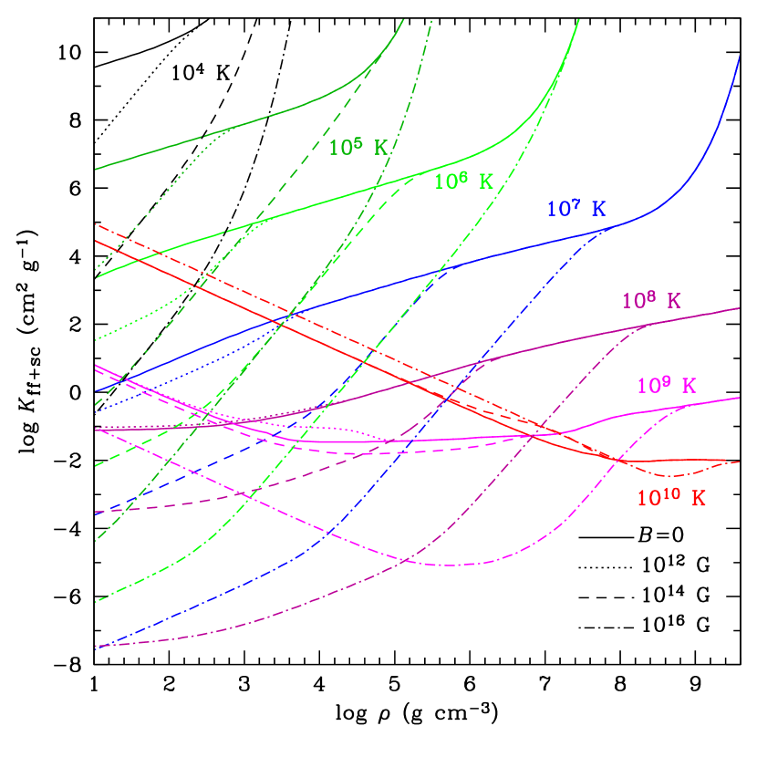
Figure 1: Rosseland mean radiative opacities due to the free-free transitions and Compton scattering in the model of fully ionized iron plasma as functions of mass density at different temperatures (marked near the curves) and magnetic fields $B=0$, $10^{12}$ G, $10^{14}$ G, and $10^{16}$ G (shown by different line styles).

3.4 Neutrino emission

Yakovlev et al. (2001) reviewed the rich variety of reactions with neutrino emission in the compact stars and presented convenient fitting formulae for applications. The rates of reactions with participation of free neutrons and protons are strongly changed if these particles are superfluid. Moreover, the very existence of nucleon superfluidity gives rise to a new neutrino emission mechanism by Cooper pair breaking and formation (PBF), most powerful at $T\sim T_{\mathrm{crit}}$.

The most important reactions in the neutron-star crust and $npe$ matter in the core with references to the appropriate fitting formulae are collected in Table 1 of Potekhin et al. (2015). In the crust, they are plasmon decay, electron-nucleus bremsstrahlung, and electron-positron annihilation. In the core, the most important reactions are different branches of direct and modified Urca processes, baryon bremsstrahlung, and the PBF at $T\sim T_{\mathrm{crit}}$. The reactions with participation of muons, fully analogous to those with the electrons, should be included for the $npe\mu$ matter. A strong magnetic field brings about additional neutrino emission processes: electron synchrotron radiation and, if protons are superconducting, bremsstrahlung due to scattering of electrons on fluxoids (Yakovlev et al. 2001).

The direct Urca processes are most powerful, but operate only if the proton fraction is large enough, which occurs above a certain threshold baryon density $\bar{n}_{\mathrm{DU}}$ (e.g., Haensel 1995). Therefore, those neutron stars whose mass $M$ exceeds a threshold $M_{\mathrm{DU}}$, where $\bar{n}$ exceeds $\bar{n}_{\mathrm{DU}}$ at the center of the star, rapidly cool down via the direct Urca processes (Lattimer et al. 1991; Page & Applegate 1992).

It is worthwhile noticing several updates in the relevant neutrino reaction rates that have been developed recently, which improve the results of Yakovlev et al. (2001). An improved fit to the emission rate due to plasmon decay, which has a larger validity range, has been constructed by Kantor & Gusakov (2007). Electron-nucleus bremsstrahlung rates for arbitrary (not only ground state) composition of the crust have been calculated and fitted by Ofengeim et al. (2014). The reduction of the neutrino emissivity of modified Urca and nucleon-nucleon bremsstrahlung processes by superfluidity of neutrons and protons in neutron-star cores has been revised by Gusakov (2002), who also presented a corrected phase-space factor for the modified Urca process in the case of a large proton fraction. Neutrino emission caused by the Cooper PBF has been recalculated by accurately taking into account conservation of the vector weak currents by Leinson & Pérez (2006) for the singlet Cooper pairing of baryons and by Kolomeitsev & Voskresensky (2008) for the triplet pairing. Leinson (2010) described a modification of the PBF neutrino emission rate due to the anomalous contribution to the axial current, arising from the off-diagonal components of the vertex matrix in the Nambu-Gorkov formalism for the nucleon interactions with the external neutrino field.

Not all of these improvements have been so far accurately included in the widely used neutron-star cooling codes and recent calculations (e.g., Page et al. 2009, 2011; Ho et al. 2015; Shternin & Yakovlev 2015; Page 2016; Taranto et al. 2016). For example, the anomalous axial PBF contribution results in a multiplication of the PBF neutrino-emission rate in the case of triplet pairing by a factor of 0.19 compared to Yakovlev et al. (2001), which is four times smaller than the factor 0.76 effectively used in the recent cooling calculations. Besides, the suppression of the contribution to the PBF emission rate in the vector channel of weak interactions (Leinson & Pérez 2006; Kolomeitsev & Voskresensky 2008) is usually taken into account by setting this contribution to zero, whereas a more accurate estimate is given by a small but non-zero multiplication factor $\sim(p_{\mathrm{F}}/m^{*}c)^{2}$, where $p_{\mathrm{F}}$ is the Fermi momentum of the relevant nucleons.

In the superdense matter of the core, the neutrino emission rates are affected by the many-body “in-medium effects” (e.g., Voskresensky 2001, and references therein). We take account of these effects following Shternin & Baldo (2017), who have obtained in-medium enhancement factors for the modified Urca emission rates. They also found an additional enhancement of the modified Urca emission rate near the threshold for the opening of the direct Urca process, which results in a non-standard temperature dependence of the emission rate $Q\propto T^{7}$, intermediate between $Q\propto T^{8}$ and $T^{6}$ for the modified and direct Urca processes, respectively.

Some neutrino emission rates can be modified by strong magnetic fields. For instance, Baiko and Yakovlev (1999) showed that the threshold for the opening of the direct Urca processes is smeared out over some $B$-dependent scale, and described this smearing by simple formulae, which we include in the present treatment of the cooling. They also showed that a strong magnetic field causes oscillations of the reaction rate in the permitted domain of the direct Urca reaction, but the latter effect, albeit interesting, appears to be unimportant for the cooling.

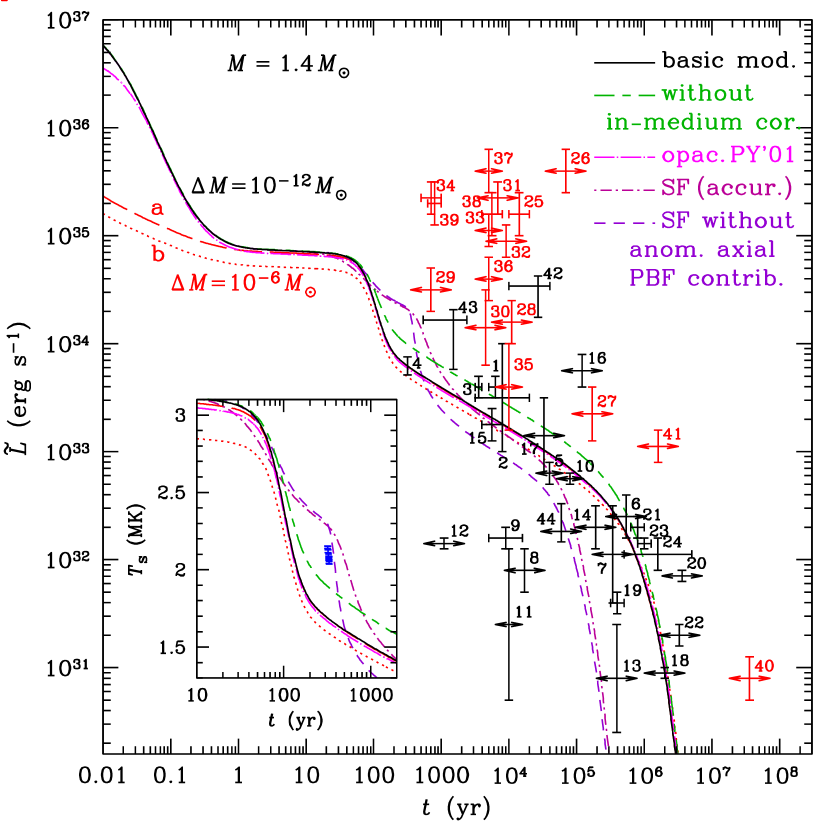
Figure 2: Theoretical cooling curves (redshifted thermal luminosity $\tilde{L}$ as a function of stellar age $t$) for a neutron star with mass $M=1.4\,M_{\odot}$, calculated using different microphysics inputs (see text for detail), versus observations of thermally emitting neutron stars. Vertical errorbars show estimated thermal luminosities, horizontal errorbars are estimated ranges of kinematic ages, short horizontal arrows replace the horizontal errorbars in the cases where no confidence interval for the kinematic age is found in the literature, and longer horizontal arrows are placed if no kinematic age is available (in such cases, the characteristic ages are adopted). Numbers 1 – 41 enumerate the entries in Table 3 of Potekhin et al. (2015). We have updated the data for object 4 according to Posselt et al. (2013) and added objects 42 (XMMU J173203.3$-$344518, Klochkov et al. 2015), 43 (CXOU J181852.0$-$150213, Klochkov et al. 2016), and 44 (PSR J0633+0632, Danilenko et al. 2015; Karpova et al. 2017). The errorbars and arrows for magnetars are drawn in red color. The inset shows the nonredshifted effective surface temperature $T_{\mathrm{eff}}$ as function of $t$ in a shorter time interval, which corresponds to the ages at which nucleon superfluidity is expected to develop in the interior of the neutron star. The symbols in the inset reproduce the data for the central compact object in the Cas A supernova remnant from Table I of Ho et al. (2015). The solid line shows the basic cooling curve, calculated using a thin quasi-stationary envelope and the most advanced physics input, except nucleon superfluidity; the long-dashed line is calculated using the same input but with a traditional (thicker) blanketing envelope treated as quasi-stationary; the dotted line is calculated using the traditional blanketing envelope and an alternative model of radiative opacities (see text); the dot-long-dashed line shows the result of replacement of the opacities shown in Fig. 1 by the simplified opacities of Potekhin & Yakovlev (2001); alternating long and short dashes demonstrate the result of neglect of the in-medium corrections; the dot-dashed cooling curve is calculated with allowance for nucleon superfluidity (one selected model for each of the three types of superfluidity: neutron singlet pairing in the crust, proton singlet and neutron triplet pairing in the core; see text for details); the short-dashed line is calculated for the same superfluidity model but without account of the anomalous axial contribution to the PBF neutrino emission.

4 Cooling of nonmagnetized neutron stars

Before considering the effects of superstrong magnetic fields on neutron star cooling, let us examine the role of the microphysics updates mentioned in Sect. 3. The solid black curve in Fig. 2 is the cooling curve of our fiducial basic model: neutron star mass $M=1.4\,M_{\odot}$, BSk24 EoS, which gives stellar radius $R=12.6$ km for this $M$, boundary layer of mass $\Delta M=10^{-12}\,M_{\odot}$, which is assumed quasi-stationary and may be partially ionized, and the physics input described in Sect. 3, but without baryon superfluidity. Although the absence of baryon superfluidity seems unrealistic, it is a convenient starting approximation for the basic model, to which all comparisons will be made.

In the main frame of the Figure we show evolution of the redshifted surface luminosity, $\tilde{L}=\mathrm{e}^{2{\Phi/c^{2}}}{L}_{R}$. Errorbars and arrows show observational estimates of the ages and thermal luminosities of 44 neutron stars with confirmed thermal emission. The first 41 sources are taken from Table 3 of Potekhin et al. (2015), and are numbered according to their order in that table, which was derived from the catalog of Viganò et al. (2013) with the addition of one source, PSR J1741$-$2054 (object number 13, Karpova et al. 2014; Marelli et al. 2014). For the thermal luminosity of the neutron star CXO J232327.9+584842 in the supernova remnant Cassiopeia A (object number 4, often dubbed Cas A NS) we have adopted improved observational data on $\tilde{L}$ (Posselt et al. 2013). We have supplemented this catalog with three neutron stars with recently measured thermal fluxes: two neutron stars with carbon envelopes (sources 42 and 43, Klochkov et al. 2015, 2016), and one pulsar (source 44, Danilenko et al. 2015; Karpova et al. 2017; in this case, we adopt the interpretation of the thermal spectrum with the model of a partially ionized magnetized hydrogen atmosphere nsmax, Ho et al. 2008). Objects 25 through 41 (red symbols) are magnetars.

The horizontal errorbars show estimates of the lower and upper bounds on the kinematic age of the star, determined from observations of the related supernova remnants. In the cases where only an estimate without errors is available, we replace the errorbar by a short double-sided arrow. In the cases where the kinematic age is unavailable, we use an estimate of the characteristic age, determined from the stellar spin period and its derivative in the canonical model of the rotating magnetic dipole in vacuum. The characteristic ages are measured very accurately, but they are rather poor estimators of a true age, therefore we plot longer horizontal arrows in these cases.

In the inset we show evolution of the nonredshifted effective temperature $T_{\mathrm{eff}}$ in a restricted time interval. Here, the points represent estimates of $T_{\mathrm{eff}}$ for the Cas A NS from Table I of Ho et al. (2015). The difference between the vertical position of these points in the inset and the errorbar 4 in the main frame is caused by the use of a different neutron star model, which gives a larger redshift and higher $T_{\mathrm{eff}}$ (see Elshamouty et al. 2013).

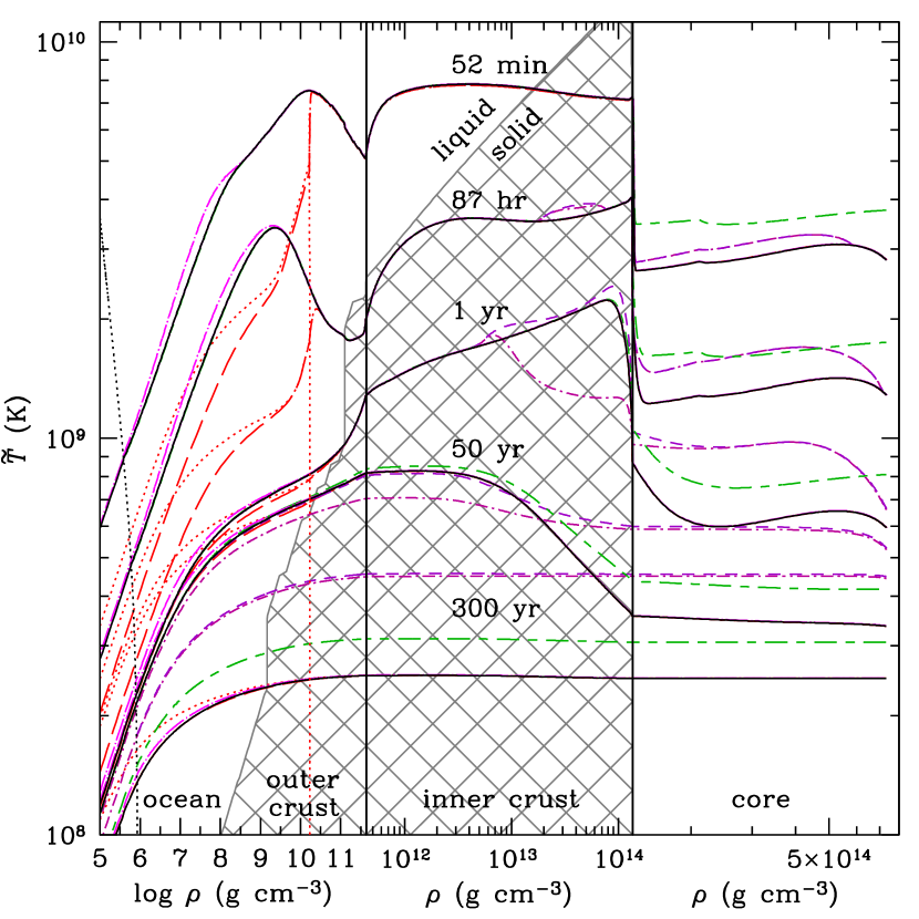
Figure 3: Redshifted temperature as a function of mass density inside a neutron star with $M=1.4\,M_{\odot}$ at different ages (marked near the curves) according to different theoretical models. Line styles correspond to theoretical models in the same way as in Fig. 2. The three parts of the Figure show the thermal structure of the envelopes comprising the ocean and the outer crust ((left), the inner crust (middle), and the core (right) at different density scales. In the gray-cross-hatched $\rho-\tilde{T}$ domain, the nuclei are arranged in a crystalline Coulomb lattice. The nearly vertical dotted lines in the left part of the Figure show the position of the outer boundary for the cooling code, beyond which (to the left in the figure) the heat transport problem is solved using quasi-stationary approximation: the left (black) and right (red) lines delimit a quasi-stationary envelope of mass $\Delta M=10^{-12}\,M_{\odot}$ and $\Delta M=10^{-6}\,M_{\odot}$, respectively.

4.1 Thickness of the quasi-stationary envelope

The cooling curves marked “a” and “b” in Fig. 2 are obtained for a model, which differs from the basic model by the thickness of the envelope that is treated in the quasi-stationary approximation, $\Delta M=10^{-6}\,M_{\odot}$ (in addition, curve “b” differs by the radiative opacity approximation, see Sect. 4.2). For the given $M$ and $R$, the mass density at the bottom of this “thick” envelope is $\rho\approx 1.7\times 10^{10}$ g cm^-3, which is close to the traditional $\rho_{\mathrm{b}}$ value. Comparison of the curve “a” with the basic cooling curve shows that the simulations with the traditional blanketing envelope are quite accurate on the timescales $t\gtrsim 1$ yr, but not on shorter timescales. The reason for this can be understood from inspection of Fig. 3, which shows temperature as function of density. At early ages the temperature profile in the thick envelope obtained in the quasi-stationary approximation (lines “a” and “b”) strongly differs from the profile calculated with the full account of time dependence in the thermal evolution equation (10) (the solid line, “basic model”). The solution of this equation in the quasi-stationary approximation is equivalent to setting $c_{P}=0$. Thus we see that the accurate evaluation of $c_{P}$ is important in the outer crust and ocean of a neutron star at relatively short timescales $t\lesssim 1$ yr.

4.2 Opacities

The influence of the model for radiative opacities on the cooling curves can be seen from comparison of the basic (solid) curve in Fig. 2 with the dot-long-dashed curve (marked “opac. PY’01”), which is calculated with simplified opacities following a model that does not include the plasma cutoff, electron-positron pairs, Compton effect, or electron degeneracy (Potekhin & Yakovlev 2001). The difference between the two cooling curves is noticeable only at high $\tilde{L}$ (the difference can exceed 10%, only if $\tilde{L}\gtrsim 10^{36.5}$ erg s^-1; in the latter case, the effect is mainly due to the importance of Compton scattering at high temperatures).

In the atmosphere, ionization can be incomplete, which is especially important in the case of heavy elements or strong magnetic fields. For the nonmagnetic iron atmosphere, we use the opal radiative opacities. There can be an ambiguity in connecting this opacity to the radiative opacity calculated in the model of a fully ionized plasma, shown in Fig. 1. In the case of the thick blanketing envelope, there are two curves in Fig. 2, long-dashed and dotted ones, corresponding to different prescriptions for the connection. The first one (curve “a”) is obtained by using the opal opacities in the density-temperature range where they are tabulated and replacing them by the fully ionized plasma model beyond the tables. The second one (curve “b”) is obtained with extrapolation of the tabular data to the bottom of the blanketing envelope, using the Kramers opacity law. The thermal structure of the envelopes with using these two prescriptions is illustrated in Fig. 3 by the red lines of the same styles (dotted and long-dashed) as corresponding lines “a” and “b” in Fig. 2. We see that these two ways of handling the radiative opacity data can result in noticeably different cooling curves, the difference being especially pronounced at $t\lesssim 100$ yr, because at early ages the radiative transport dominates in a large part of the envelope due to the high temperatures.

4.3 Anomalous axial PBF contribution

To check the importance of the recent advances in the treatment of the Cooper PBF neutrino emission mechanism, we first include the superfluidity with the accurate treatment of this emission mechanism according to Leinson (2010) (the dot-dashed lines in Figs. 2 and 3), and then switch off the anomalous contribution into the axial channel of weak interactions (the short-dashed lines). For illustration, we have chosen the superfluidity type SF081326. Here and hereafter, the first (08), second (13), and third (26) pair of digits compose the entry number in Table II of Ho et al. (2015). Thus, SF081326 stands for the superfluid gap model SFB for the neutron singlet superfluidity (Schwenk et al. 2003), CCDK for the proton singlet superfluidity (Chen et al. 1993; Elgarøy et al. 1996a), and TToa for the neutron triplet superfluidity (Takatsuka & Tamagaki 2004). This combination has been selected by Ho et al. (2015) as the best fit to the apparent surprisingly rapid decline of luminosity of the Cas A NS, first reported by Heinke & Ho (2010). In the inset of Fig. 2 we can see that the short-dashed curve $T_{\mathrm{eff}}(t)$ is indeed close to the plotted Cas A NS data in the common approximation neglecting the anomalous axial contribution, but it is not the case if the PBF emission is calculated accurately. This conclusion confirms the statement by Leinson (2016) about the importance of the latter contribution.

Let us note that Shternin et al. (2011) were the first who encountered the impossibility of fitting the apparent fast decline of the Cas A NS luminosity with the results of Leinson (2010). In order to obtain an acceptable fit to this decline, they (as later Elshamouty et al. 2013) arbitrarily increased the PBF reaction rate by changing the coefficient 0.19, mentioned in Sect. 3.4, to 0.4, which does not follow from any theory. This artificial enhancement of the PBF rate is however unnecessary, since the fast cooling of Cas A NS has been put in doubt by Posselt et al. (2013), who suggested possible alternative explanations to the observational data.

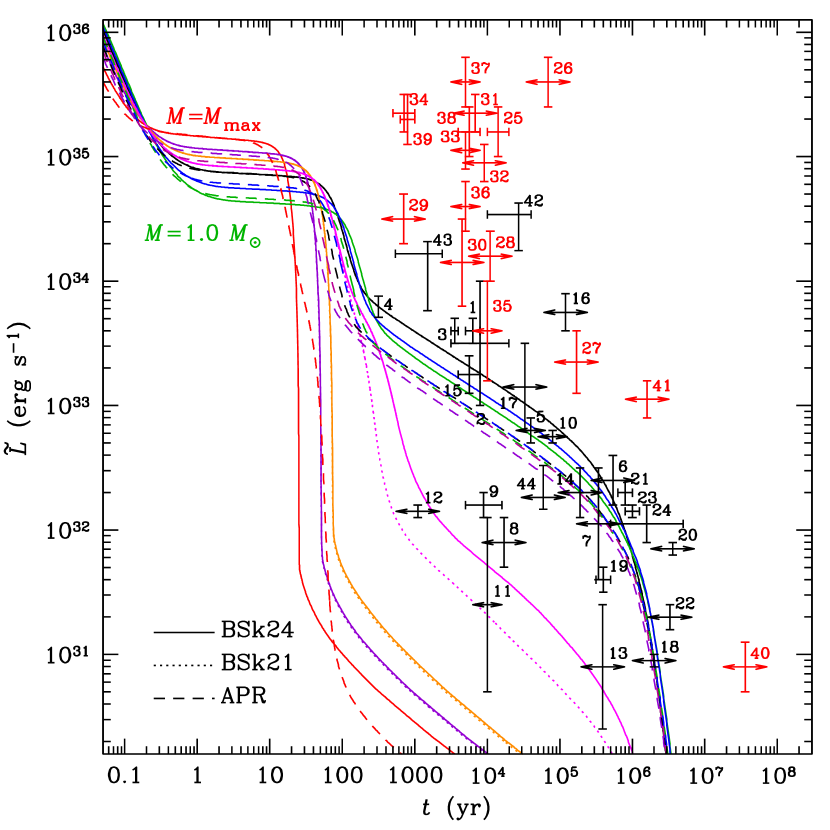
Figure 4: The cooling curves for neutron stars with $M=1.0$ (green), 1.2 (blue), 1.4 (black), 1.6 (magenta), 1.8 (orange), $2.0\,M_{\odot}$ (violet), and the maximum mass $M_{\mathrm{max}}$ (red lines), calculated using the same basic theoretical model as in Fig. 2, for the EoS models BSk24/21 (solid/dotted lines, $M_{\mathrm{max}}=2.28\,M_{\odot}$, $M_{\mathrm{DU}}=1.596/1.587\,M_{\odot}$) and APR+NV (dashed lines, $M_{\mathrm{max}}=2.21\,M_{\odot}$, $M_{\mathrm{DU}}=2.01\,M_{\odot}$) compared with observations (the same symbols as in Fig. 2).

4.4 In-medium effects

The importance of the in-medium effects can be seen from comparison of the corresponding cooling curves in Fig. 2 and temperature profiles in Fig. 3. Simulations without account of these effects substantially overestimate luminosities and effective temperatures of middle-aged neutron stars. We have checked that this effect is caused mainly by the in-medium enhancement of the modified Urca reactions (Shternin & Baldo 2017). The in-medium effects on thermal conductivities (Baiko et al. 2001; Shternin et al. 2013) turn out to be unimportant.

4.5 Equation of state and direct Urca processes

Figures 4 and 5 illustrate the effects of varying neutron star mass and equation of state on the cooling curves and thermal structure of neutron stars. In Fig. 4 we show a sequence of cooling curves for stellar masses $M$ from $1.0\,M_{\odot}$ to $2.0\,M_{\odot}$ and the maximum mass $M_{\mathrm{max}}$, according to two EoSs, BSk24 ($M_{\mathrm{max}}=2.28\,M_{\odot}$) and APR ($M_{\mathrm{max}}=2.21\,M_{\odot}$).

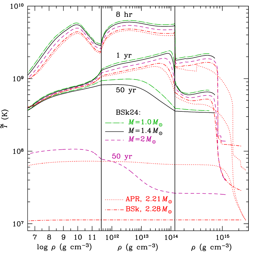
Figure 5: Redshifted temperature as function of mass density inside neutron stars with masses $M=1.0$ (dot-long-dash lines), 1.4 (solid lines), 2.0 (short-dashed lines), and $M_{\mathrm{max}}=2.28\,M_{\odot}$ (dot-short-dash lines) for the unified EoS model BSk24, and with mass $M_{\mathrm{max}}=2.21\,M_{\odot}$ for the APR+NV EoS model (dotted lines) at ages of $10^{-3}$, 1, and 50 years. The vertical lines separate three density regions: the ocean and outer crust, the inner crust, and the core, displayed using different density scales.

The cooling curves are close to the basic curve until $M$ exceeds the direct Urca threshold $M_{\mathrm{DU}}$, which is equal to $1.596\,M_{\odot}$ for BSk24 and to $2.01\,M_{\odot}$ for APR. The difference of $M_{\mathrm{DU}}$ for different EoSs is caused by different density-dependence of the electron fraction, which is obtained along with the thermodynamic functions while calculating the EoS by the free energy minimization. For $M>M_{\mathrm{DU}}$, a powerful cooling occurs in the central part of the core.

We have also performed analogous calculations for the EoS model BSk21, but found that the results are almost indistinguishable from those obtained with BSk24, except for values of $M$ close to $M_{\mathrm{DU}}$. In Fig. 4, the difference is noticeable only for $M=1.6\,M_{\odot}$ (the dotted curve). This is because the sensitivity of the cooling to the mass of the central region where the direct Urca processes operate. For BSk21, $M_{\mathrm{DU}}=1.587\,M_{\odot}$, the threshold at $M=1.6\,M_{\odot}$ is exceeded by $M-M_{\mathrm{DU}}=0.013\,M_{\odot}$, compared to $0.004\,M_{\odot}$ for BSk24. A change of $M$ by $-0.009\,M_{\odot}$ brings the dotted cooling curve in Fig. 4 to the solid one. Such a small difference in $M$ seems to be practically insignificant.

Figure 5 shows temperature profiles for several masses and ages. We see that some of the red and magenta lines go down towards the right edge of the Figure, indicating temperature decrease with increasing density towards the center of the most massive stars. At early ages ($t\lesssim 1$ yr), this temperature decrease exceeds an order of magnitude for the models with $M=2\,M_{\odot}$ and $M=M_{\mathrm{max}}$ using the BSk24 EoS and for the model with $M=M_{\mathrm{max}}$ using the APR EoS. Thus the central region of the massive neutron star works as a cooler. As seen from Fig. 5, it is effective until the temperature falls to $\sim 10^{7}$ K. Afterwards the neutrino cooling dyes away and the temperature profile flattens out.

The total neutrino emissivities for several neutron star models and two ages are shown in Fig. 6. We see that for $M=1.8\,M_{\odot}>M_{\mathrm{DU}}$(BSk24) the emission rate at $\rho>8.25\times 10^{14}$ g cm^-3 is enhanced by several orders of magnitude compared to the rates at lower densities.

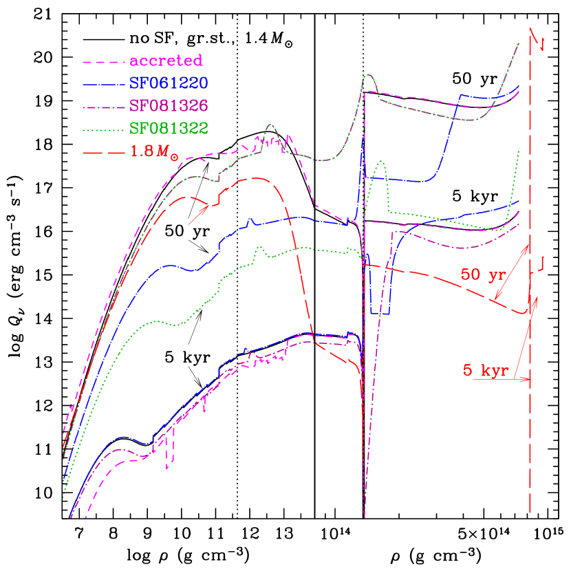
Figure 6: Neutrino emission power density as function of mass density at ages 50 yr (upper curves) and 5 kyr (lower curves of each type) for different neutron star models: the basic model (EoS BSk24, ground state composition, $M=1.4\,M_{\odot}$, no superfluidity; solid lines), the neutron star with fully accreted envelope (short-dashed lines), three different combinations of the three types of superfluidity (dot-long-dash, dot-short-dash, and dotted curves), and a model without superfluidity but with the direct Urca processes due to the higher mass $M=1.8\,M_{\odot}$ (long-dashed lines). The density scale is different in the left and right parts of the Figure, separated by the vertical solid line. The vertical dotted lines mark the outer and inner boundaries of the inner crust.

4.6 Superfluidity

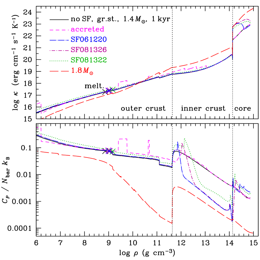
Figure 7: Thermal conductivity (upper panel) and heat capacity per baryon in units of $k_{\mathrm{B}}$ (lower panel) as functions of mass density at age $t=1$ kyr for the same neutron star models as in Fig. 6. The crosses mark the melting points for the models with $M=1.4\,M_{\odot}$: to the left of them, the Coulomb plasma forms a liquid ocean. For the $M=1.8\,M_{\odot}$ model, the crust does not melt in the displayed density range, because it is relatively cold at this age (cf. Fig. 4). The vertical dotted lines mark the outer and inner boundaries of the inner crust.

It is well known that superfluid energy gaps for different types of nucleon pairing have an important influence on the neutron star-cooling curves. When temperature falls substantially below $T_{\mathrm{crit}}$ for some kind of the baryons, the superfluidity reduces their heat capacity (Levenfish & Yakovlev 1994; Yakovlev et al. 1999). The baryon superfluidity may also either reduce or increase the conductivity in the core (Baiko et al. 2001). These effects are seen respectively in the lower and upper panels of Fig. 7.

The baryon superfluidity affects the neutrino emissivity in different ways (Yakovlev et al. 2001, and references therein). Neutrino emission by the modified and direct Urca processes and by baryon bremsstrahlung gets strongly suppressed at $T\ll T_{\mathrm{crit}}$. However, when $T$ is close to $T_{\mathrm{crit}}$, the total neutrino emission is greatly enhanced due to the PBF mechanism. Since $T_{\mathrm{crit}}$ for each type of superfluidity depends on baryon density, the overall picture is complicated, as we see in Fig. 6.

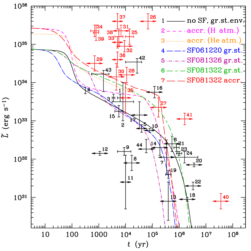
Figure 8: Cooling curves for a neutron star with $M=1.4\,M_{\odot}$ according to the BSk24 EoS model with iron (lines 1, 4, 5, 6) or accreted envelopes (lines 2, 3, 7), iron (lines 1, 4, 5, 6), hydrogen (lines 2, 7), or helium atmosphere (line 3), without nucleon superfluidity (lines 1 – 3) and with different models of nucleon superfluidity (lines 4 – 7; see text for explanation of the SF-notations), compared with observations (the same symbols as in Fig. 2).

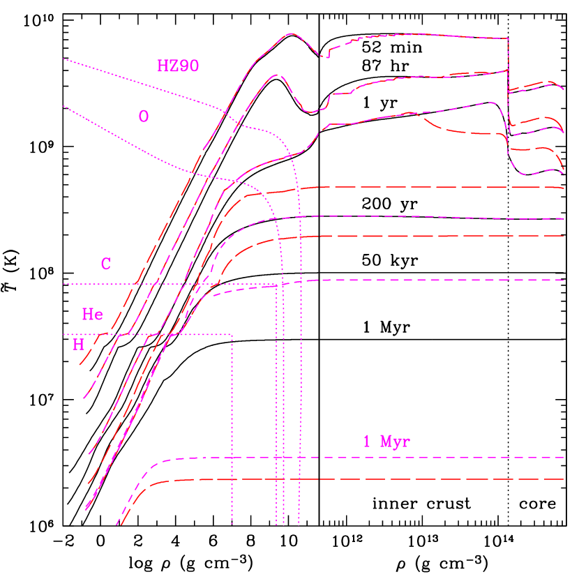
Figure 9: Redshifted temperature as a function of mass density inside a neutron star for three of the seven different models considered in Fig. 8 (namely, models 1, 2, and 7), plotted using the same line styles, at different ages marked near the curves. The two parts of the Figure, separated by the vertical solid line, show the regions before and after neutron drip at different density scales. The dotted lines in the left half of the Figure show the adopted density-temperature domains for different chemical elements (H, ⁴He, ¹²C, ¹⁶O) in the accreted envelope. To the right of the last of these lines, the composition of the accreted crust is adopted from Haensel & Zdunik (1990). For the nonaccreted crust, we use the ground-state composition of matter according to the BSk24 model. The vertical dotted line in the right half of the Figure separates the crust and the core.

As a result, some parts of a neutron star may have higher- while other parts lower temperature than it would be for a neutron star without superfluidity. We see this in Figs. 3 and 9, which show temperature profiles in superfluid and nonsuperfluid neutron stars of different ages. The cooling can be accelerated or decelerated, depending on the interplay of the superfluidity-related mechanisms, as we see in Fig. 8 where the effects of three different models of superfluidity are demonstrated.

The model SF081326, which is also used in Figs. 2 and 3, is characterized by a relatively weak neutron singlet-pairing superfluidity SFB in the crust (maximum of the critical temperature $\max T_{\mathrm{crit}}\sim 5\times 10^{9}$ K), rather strong proton singlet superfluidity CCDK in the core ($\max T_{\mathrm{crit}}\approx 7\times 10^{9}$ K), and moderate neutron triplet superfluidity TToa in the core ($\max T_{\mathrm{crit}}\approx 6\times 10^{8}$ K). In Fig. 8 we reproduce the corresponding cooling curve (line 4) and compare it with the curves calculated using two different combinations of the superfluidity models (lines 5 and 6). Retaining the same singlet-type superfluidities but replacing the moderate neutron triplet model TToa by the weak neutron triplet superfluidity model EEHOr with $\max T_{\mathrm{crit}}<2\times 10^{8}$ K (Elgarøy et al. 1996b), we effectively suppress the PBF neutrino emission at moderate ages, which helps to keep a neutron star relatively hot for a long time (curves 6 and 7 in Fig. 8). This model is sufficient for explanation of several sources showing luminosities above those predicted by the basic cooling curve; nevertheless, there remain many still hotter neutron stars, which require another explanation.

As another example, we choose model combination SF061220: the strong neutron singlet superfluidity MSH ($\max T_{\mathrm{crit}}>10^{10}$ K, Margueron et al. 2008; Gandolfi et al. 2009), moderate proton singlet superfluidity BS ($\max T_{\mathrm{crit}}\sim 5\times 10^{9}$ K, Baldo and Schulze 2007), and moderate neutron triplet superfluidity BEEHS ($\max T_{\mathrm{crit}}\sim 4\times 10^{8}$ K, Baldo et al. 1998). In this case, cooling is accelerated at early and late ages (line 4 in Fig. 8).

4.7 Accreted envelopes

The neutron star envelopes are more transparent to the heat flux if they are composed of light chemical elements. Previously we studied this effect in the quasi-stationary approximation for nonmagnetic (Potekhin et al. 1997) and strongly magnetized envelopes (Potekhin et al. 2003). The main effect is related to the $Z$-dependence of the electron-ion collision frequencies. The higher the ion charge number $Z$, the larger the collision frequency and the lower the conductivity. Another effect concerns radiative opacities in the photosphere, which are also smaller for light elements than for iron.

Here we more accurately simulate the cooling of neutron stars with accreted envelopes by relaxing the quasi-stationary approximation. The cooling curves for nonsuperfluid (lines 1 – 3) and superfluid (lines 4 – 7) neutron stars with nonaccreted (lines 1, 4, 5, 6) and accreted (lines 2, 3, 7) envelopes are compared in Fig. 8 and their thermal structures are shown in Fig. 9.

For the accreted envelopes, we use either hydrogen (lines 2 and 7) or helium (line 3) atmosphere models. An interesting effect, first noticed by Beznogov et al. (2016), is that the replacement of H by ⁴He increases the photon luminosity. This effect is caused by the different mass to charge ratio of H, which results in the discontinuity of $\rho$ and is related to the lower opacities of He at high $T$and fixed $\rho$, revealed in both op and opal tables. These discontinuities are seen in the left part of Fig. 9 at the H/He interface, which is set at $T=4\times 10^{7}$ K ($\tilde{T}\approx 3.3\times 10^{7}$ K), for the accreted-envelope models (dashed lines). On the other hand, the kinks at the temperature profiles for nonaccreted envelopes (solid lines in Fig. 9) at $\tilde{T}\lesssim 3\times 10^{7}$ K are caused by the switch to the fully ionized plasma model for radiative opacities at the boundary of the opal tables for iron (see Sect. 4.2).

The composition of the accreted crust at larger densities, beyond the C and O layers, is produced by a sequence of nuclear transformations during accretion (Haensel & Zdunik 1990). This leads to different thermal conductivities and heat capacities, as seen in Fig. 7, and to different rates of neutrino bremsstrahlung, as seen in Fig. 6. The latter differences, however, are not sufficiently strong to noticeably affect the cooling curves.

Figure 8 shows that the largest theoretical luminosities are obtained by the use of the model with strong proton singlet and weak neutron triplet superfluidity (SF081322) and the accreted He envelope.

4.8 Other effects

We have additionally tested a number of other updates to the neutron star microphysics, which however proved to be unimportant. Two examples, the in-medium corrections to thermal conductivities and the upgrade of the BSk21 to the BSk24 EoS, have been mentioned above. Another example is latent heat of the crust. As a neutron star cools down, its frozen crust grows, gradually replacing the ocean. We have included the latent heat released during this process as a heat source $\tilde{H}$ in Eq. (10), but found the cooling curves unchanged. This should have been anticipated, because the crust contains only a small fraction (less than 2%) of the total mass $M$ of a neutron star.

The replacement of the fit of Yakovlev et al. (2001) to bremsstrahlung neutrino energy losses in the crust by a more detailed fit of Ofengeim et al. (2014) also does not affect the cooling curves, even in the case of accreted crust

We have also checked that the replacement of the fit of Yakovlev et al. (2001) to the plasmon decay rate by the more accurate fit of Kantor & Gusakov (2007) does not have a noticeable effect on the cooling curves (this statement pertains to neutron stars, but not to white dwarfs, where the plasmon decay is an important channel of energy losses at early ages).

5 Cooling of magnetars

The effects of quantizing magnetic fields on the thermal structure of neutron-star envelopes were first studied by Hernquist (1985) and somewhat later by Van Riper (1988) and Schaaf (1990). Van Riper (1988) considered a neutron star with a constant radial magnetic field. In this model, the quantum enhancement of longitudinal electron conductivity $\kappa_{\|}$ at $\rho\sim\rho_{B}$ (where $\rho_{B}$ is given by Eq. (12)) results in an overall enhancement of the neutron-star photon luminosity at a fixed internal temperature. However, Shibanov & Yakovlev (1996) showed that, for the dipole field distribution, the effects of suppression of the heat conduction across the field near the magnetic equator compensate or even overpower the effect of the conductivity increase near the normal direction of the field lines. This conclusion was also shown to be valid for small-scale fields at $B\lesssim 10^{14}$ G (Potekhin et al. 2005). However, in superstrong fields $(B\gtrsim 10^{14}$ G) the quantum enhancement of the longitudinal conductivity and the corresponding increase of the stellar photon luminosity are more important. This enhancement overpowers the decrease of the luminosity in the regions of almost tangential field lines, so that overall photon luminosity increases (Kaminker et al. 2009, 2014). This may not be the case in the configurations where the field is nearly tangential over a significant portion of the stellar surface as, for example, in the case of a superstrong toroidal field (Pérez-Azorin et al. 2006; Page et al. 2007). We do not study the latter possibility in the present paper, assuming that the superstrong magnetar field is highly tangled.

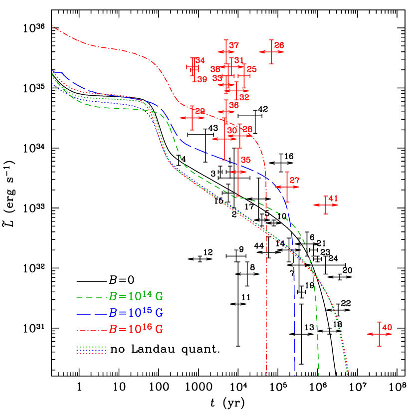
Figure 10: Cooling curves for neutron stars with $M=1.4\,M_{\odot}$ according to the BSk24 EoS model with $B=0$ (solid line), $10^{14}$ G (short-dashed line), $10^{15}$ G (long-dashed line), and $10^{16}$ G (dot-dashed line). The three dotted lines result from simulations with the same three strong fields, but treated classically.

Figure 10 shows cooling curves of neutron stars with $B=10^{14}$ G, $10^{15}$ G, and $10^{16}$ G, compared with the cooling of a nonmagnetic neutron star. We see the strong enhancement of the luminosity for middle-aged neutron stars with superstrong magnetic fields. As a consequence of rapid energy loss, the stored thermal energy is spent more rapidly, and the luminous lifetime of the magnetars becomes shorter. We intentionally leave aside additional heating by the magnetic energy consumption (e.g., by one of the mechanisms considered by Beloborodov & Li 2016), which may become the subject of a separate study. Here we aim at revealing the luminosity increase that can be provided by the effects of the quantizing magnetic fields on the crust of the star.

For comparison, we plot the cooling curves obtained using classical treatment of the magnetic fields (i.e., without allowance for the Landau quantization). At the middle ages of the stars, the latter curves pass below the nonmagnetic curve, which is explained by the magnetic suppression of the electron heat transport across the field lines.

Figure 11 shows thermal structure of magnetars at different ages. For comparison, we reproduce the thermal structure of a nonmagnetized neutron star with iron envelopes from Sect. 4. The temperature profiles of the strongly magnetized neutron stars reveal series of kinks, which are related to the magnetic quantization. They are located near the points where degenerate electrons fill consecutively excited Landau levels at densities $\rho\gtrsim\rho_{B}$. At these densities, the average conductivities have peaks and dips, as shown in Fig. 12.

Only part of the enhancement of luminosity in Fig. 10 is due to the above-mentioned increase of conductivity at $\rho\sim\rho_{B}$. Equally important is the magnetic condensation, the phenomenon predicted by Ruderman (1971) and studied by Lai & Salpeter (1997) and Medin & Lai (2006, 2007). In a nonmagnetized dense nonideal electron-ion plasma, the pressure of degenerate electrons overpowers the negative electrostatic pressure at high densities. In the superstrong fields of magnetars, however, the Fermi temperature is so strongly reduced at $\rho\ll\rho_{B}$, that the electrons become nondegenerate, and hydrostatic instability develops, leading to formation of a condensed surface at high density. The radiation escapes directly from this hot surface, without diffusion through a gaseous atmosphere. Such a neutron star is said to be “naked” (Turolla et al. 2004).

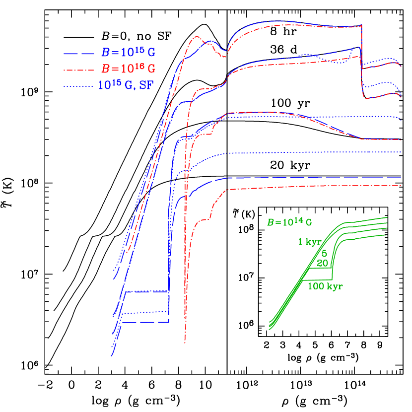
Figure 11: Redshifted temperature as a function of mass density inside neutron stars with $B=0$ (solid lines), $10^{15}$ G (long-dashed and dotted lines), and $10^{16}$ G (dot-dashed lines) at four ages $t$ from 8 hours to $2\times 10^{4}$ years, marked near the curves. The dotted line illustrates the model with superfluidity SF081322; the other lines are calculated without superfluidity. The two parts of the Figure, separated by the vertical solid line, show the regions before and after neutron drip at different density scales. Inset: temperature profiles in the envelopes of a neutron star with $B=10^{14}$ G at ages $t=1$, 5, 20, and 100 kyr.

The process of formation of the naked neutron star is elucidated by Fig. 11. At early times, when a magnetar is sufficiently hot, its thermal structure is smooth because it possesses a thick atmosphere. As the magnetar cools down, a sharp condensed surface appears. Nevertheless, in the case of $B=10^{15}$ G, we see that the neutron star retains a finite atmosphere with densities $\rho\gtrsim 10^{3}$ g cm^-3 above the condensed surface.

The inset in Fig. 11 illustrates the structure of the envelopes of a neutron star with $B=10^{14}$ G at the middle ages $t=10^{4\pm 1}$ yr, around the time of magnetic condensation. The two upper profiles are smooth, without a condensed surface, and the two lower curves reveal a density gap, which corresponds to an atmosphere and ocean above a dense solid crust. As the star cools down, the ocean depth decreases. The condensation is accompanied by increasing heat-transparency of the envelope. For this reason, the decrease of the surface luminosity stalls, and the two profiles in the middle (at $t=5$ kyr and 20 kyr, before and after the condensation) are close to each other at low densities. The slowdown of the luminosity decrease is clearly distinguishable on the cooling curve for $B=10^{14}$ G at $t\sim 10^{4}$ yr in Figs. 10 and 14.

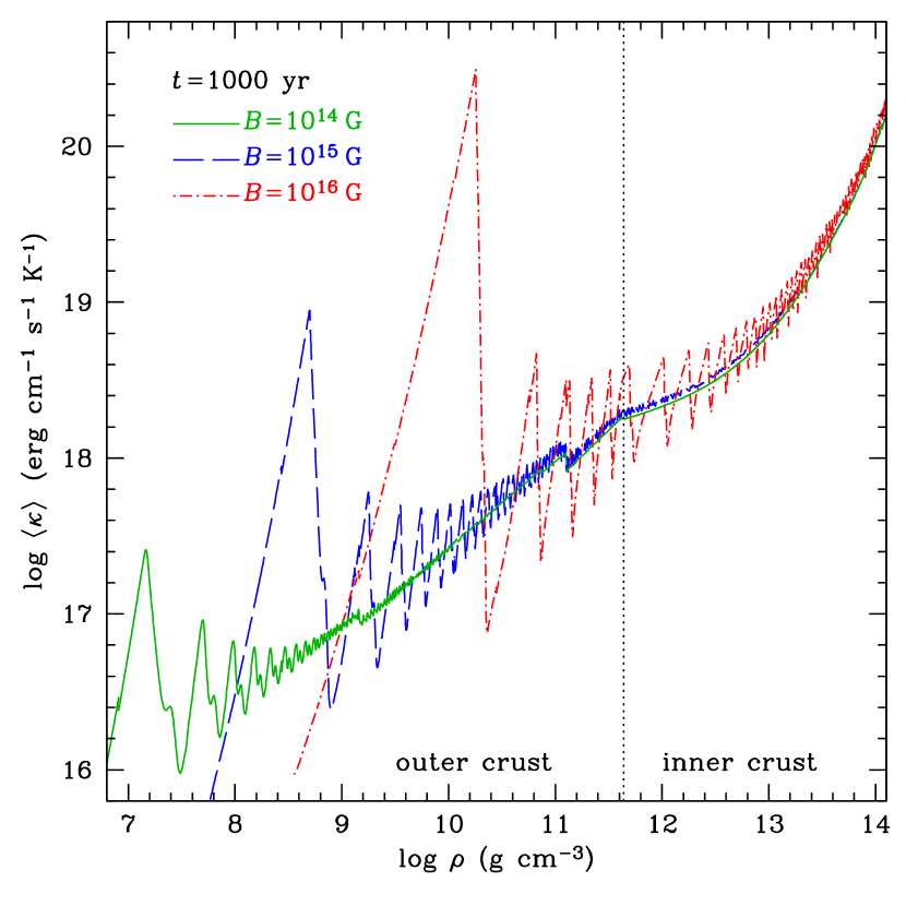
Figure 12: Effective thermal conductivity as a function of density in the ocean and crust of a kyr-old magnetar with magnetic fields $B=10^{14}$ G, $10^{15}$ G, and $10^{16}$ G. The vertical dotted line marks the neutron drip density.

Figure 13 shows neutrino emission rates inside nonsuperfluid magnetars with $B=10^{14}$ G, $10^{15}$ G, and $10^{16}$ G and a magnetar with superfluidity type SF081322 and $B=10^{16}$ G. For reference, neutrino emission of the basic nonmagnetic neutron star model is also shown. For ease of comparison with Fig. 6, we have chosen the same two ages, 50 yr and 5 kyr, and the same scale as in that Figure. The most remarkable difference is the enhanced emission in the inner crust for $B=10^{14}$ G and $10^{15}$ G. The increase is due to the contribution of the synchrotron neutrino emission. At the strongest considered field $B=10^{16}$ G, however, the synchrotron contribution disappears, which looks surprising at the first glance. Actually the synchrotron emission is quenched at $T\ll T_{B}=T_{\mathrm{cycl}}/\sqrt{1+x_{\mathrm{r}}^{2}}$ (Bezchastnov et al. 1997), where $T_{\mathrm{cycl}}$ is the electron cyclotron temperature defined in Sect. 3 and $x_{\mathrm{r}}=p_{\mathrm{F},\mathrm{e}}/m_{\mathrm{e}}c$ is the usual parameter of relativity. At $B=10^{16}$ G the condition $T\ll T_{B}$ is fulfilled in the inner crust. The quenching is described by a factor $S_{\mathrm{BC}}$ in Sect. 2.4b of Yakovlev et al. (2001), which is exponentially small at $T_{B}/T\gg 1$.

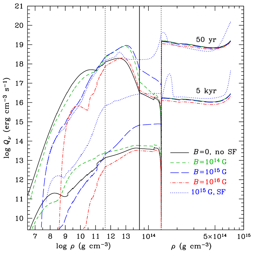
Figure 13: Neutrino emission power density as a function of mass density at ages 50 yr (upper curves) and 5 kyr (lower curves of each type) for nonsuperfluid magnetars with $B=10^{14}$ G (short-dashed lines), $10^{15}$ G (long-dashed lines), and $10^{16}$ G (dot-dashed lines) and for a magnetar with $B=10^{15}$ G and nucleon superfluidity (dotted lines), compared with neutrino emission of a nonmagnetic, nonsuperfluid neutron star (solid lines). The density scale is different in the left and right parts of the Figure, separated by the vertical solid line. The vertical dotted lines mark the outer and inner boundaries of the inner crust.

We have seen that strong proton superfluidity in the core, accreted envelopes, and superstrong magnetic fields enhance luminosities of neutron stars at $t\sim 10^{2}-10^{4}$ yr. One might expect that joint effect of these factors would help to explain observations of the most luminous magnetars. However, this is not the case. Figure 14 shows cooling of magnetars without and with strong proton superfluidity along with an example of a superfluid magnetar with an accreted envelope. We see that the stronger the magnetic field, the smaller the additional enhancement of the photon luminosity due to the superfluidity. Replacement of the iron envelope by an accreted envelope does not produce any appreciable effect on the cooling of those magnetars, whose luminosity has been already enhanced by a magnetic field $B\gtrsim 10^{15}$ G and strong proton superfluidity.

The cooling curves in Fig. 14 are compatible with the observed luminosities and estimated ages of several magnetars without involving heating mechanisms. However, most of the data on magnetars are barely compatible with the theoretical cooling curves, and several objects (e.g., objects number 26, 4U 0142+614; 37, SGR 0526$-$66; 40, SGR 0526-66) are clearly incompatible with them. This indicates that heating mechanisms are probably important for the thermal evolution of magnetars, in agreement with previously published conclusions (e.g., Kaminker et al. 2009; Viganò et al. 2013; Beloborodov & Li 2016). Nonetheless, Fig. 14 demonstrates that combined effects of Landau quantization, magnetic condensation, and strong proton superfluidity substantially reduce the discrepancies without resorting to accreted envelopes of light elements, which would hardly survive on the surface of magnetars, due to high temperatures and bursting activity.

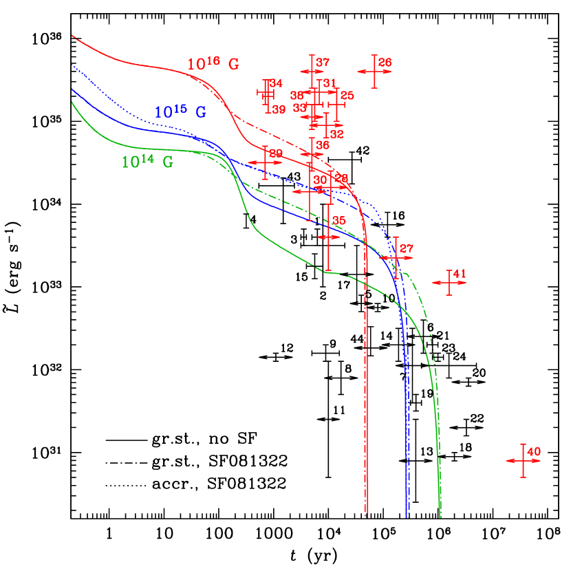
Figure 14: Comparison of cooling of nonsuperfluid (solid lines) and superfluid (dot-dashed lines) magnetars with superfluidity type SF081322 and magnetic fields $B=10^{14}$ G, $10^{15}$ G, and $10^{16}$ G. The dotted line shows the joint effect of superfluidity and accreted envelope for the magnetar with $B=10^{15}$ G.

6 Conclusions

We have performed simulations of cooling of nonmagnetic neutron stars and neutron stars with tangled superstrong magnetic fields. We have studied the influence of various recent updates to microphysics input and the effects brought about by superstrong magnetic fields of magnetars. We treat the fully ionized envelopes uniformly with the interior of the star while taking into account the $T$-dependence of the EoS in the outer crust. We have considered both neutron stars with ground-state composition and with accreted envelopes.

We demonstrate that cooling simulations based on the approximation of a quasi-stationary envelope, which extends to $\rho_{\mathrm{b}}\sim 10^{10}$ g cm^-3, are accurate on the timescales $\gtrsim 1$ yr, but not on the shorter timescales. The accurate treatment of the PBF neutrino emission, including the effect of suppression of axial channel for triplet type of Cooper pairing of neutrons, caused by contribution of the anomalous weak interaction (Leinson 2010), can be important. In particular, it is shown that the inclusion of this effect invalidates the tentative explanation of the apparent rapid cooling of the Cas A NS by the PBF emission mechanism (Page et al. 2011; Ho et al. 2015), in agreement with Leinson (2016). The enhancement of the Urca reactions by the in-medium effects (Voskresensky 2001; Shternin & Baldo 2017) are equally important.

On the other hand, the latent heat of the crust, the in-medium effects on baryon thermal conduction, the upgrade of BSk21 to BSk24 EoS model, and the recent improvements in treatments of neutrino bremsstrahlung and plasmon decay in the crust proved to have almost no effect on the cooling. Allowance for the electron-positron pairs, electron degeneracy, Compton effect, and plasma cutoff in the treatment of radiative opacities can noticeably (by $>10$%) improve accuracy of the simulations of thermal evolution only for very hot neutron stars, with photon luminosities above $10^{36}$ erg s^-1, and are unimportant for colder sources.

In agreement with previous studies, we find that accreted envelopes and superstrong magnetic fields make the neutron-star envelope more heat-transparent, which results in an increase of the surface luminosity at the neutrino cooling stage and quick fading at a later photon cooling stage. The cooling can be decelerated at the middle ages by a combination of weak neutron and strong proton superfluidities. However, the effects of the accreted envelopes and superstrong magnetic fields are not additive. Thus the highest luminosity of a cooling magnetar (without heating sources) at the middle ages $t\sim 10^{4}$ yr is provided by the superstrong magnetic field and superfluidity without an accreted envelope. This maximum luminosity is still not sufficient to explane observations of the most luminous magnetars, which implies the importance of heating. A study of the magnetar heating problem is beyond the scope of the present paper.

We did not consider magnetic fields stronger than $10^{16}$ G for two reasons; First, the strongest observed dipole component of a magnetic field of a neutron star, evaluated from the star spindown rate, is $2\times 10^{15}$ G. While several times stronger small-scale fields look plausible, orders of magnitude stronger fields do not. The second reason is more fundamental. At $B>10^{16}$ G, a number of physical effects come into play, which can be safely neglected at lower fields and have not been included in the present study. Examples of such effects are the $B$-dependence of the neutron drip transition pressure (Chamel et al. 2016), a possible influence of the field on nuclear shell energies and magic numbers, which may substantially change the composition and structure of the crust (Kondratiev et al. 2000, 2001; Stein et al. 2016), and the shift of the muon production threshold in the core (Suh & Mathews 2001).

Appendix A Analytical parametrizations at $B=0$

For modeling stellar structure and evolution, analytical parametrizations of the quantities of astrophysical interest can be useful. We have constructed such parametrizations for the BSk24 and APR EoS models, following the approach previously developed by Haensel & Potekhin (2004) for Sly4 EoS and Potekhin et al. (2013) for BSk21 EoS. The unified fits to pressure and energy density cover a broad density range including the inner crust and the core. These unified fits smear away all density discontinuities between layers of different composition. Other quantities that are required in modeling neutron-star structure and evolution, such as particle fractions, are given by separate parametrizations for the inner crust and the core.

In the case of BSk24, the analytical fitting formulae for pressure $P$ as a function of mass density $\rho$, energy per baryon as a function of baryon number density $\bar{n}$, number fractions of the electrons $Y_{\mathrm{e}}$ in the core and free nucleons ($Y_{\mathrm{n}}$, $Y_{\mathrm{p}}$) in the inner crust, sizes and shapes of nuclei in the inner crust, chemical potentials of neutrons and protons in the inner crust and the core will be presented in Pearson et al. (2017). We do not reproduce them here, but refer the reader to the web site, dedicated to Fortran implementations of the EoS fits mentioned in this Appendix.

For the APR EoS, we have constructed parametrizations of pressure and density in exactly the same form as those presented by Haensel & Potekhin (2004) for the SLy4 EoS model of Douchin & Haensel (2001) in a wide density range including the core and crust. Since APR does not apply in the crust, the present unified fits rely on the SLy4 EoS at $\bar{n}<\bar{n}_{\mathrm{cc}}$, where $\bar{n}_{\mathrm{cc}}$ is the baryon number density at the crust-core transition ($\bar{n}_{\mathrm{cc}}=0.075959$ fm^-3 according to Douchin & Haensel 2001).

The parametrization of pressure $P$ as a function of mass density $\rho$ is

$$\!\!\!\!\!\log_{10}\left(\frac{P}{\mbox{dyn cm${}^{-2}$}}\right)=\frac{6.22+6.121\xi+0.006035\,\xi^{3}}{(1+0.16354\,\xi)\big{[}\mathrm{e}^{4.73\,(\xi-11.5831)}+1\big{]}}$$

$$\qquad+\frac{12.589+1.4365\,\xi}{\mathrm{e}^{4.75\,(11.5756-\xi)}+1}+\frac{3.8175\,\xi-42.489}{\mathrm{e}^{2.3\,(14.81-\xi)}+1}$$

$$\qquad+\frac{29.80-2.976\,\xi}{\mathrm{e}^{1.99\,(14.93-\xi)}+1},$$ (14)

where $\xi\equiv\log_{10}(\rho/\textrm{g cm}^{-3})$. The typical fit error of $P$ is $\approx 1-2$% for $6\lesssim\xi\lesssim 16$; the maximum error of $\lesssim 4$% is due to the continuous fitting across the discontinuity of density at the phase boundary between the crust and the core.

The mass density $\rho$ and the baryon number density $\bar{n}$ are approximated as functions of each other by the formulae

$$\frac{n_{0}}{\bar{n}} = 1+\left(0.342\bar{n}^{2.23}+2.2\times 10^{-6}\bar{n}^{10.92}\right)\left(1+a_{\mathrm{n}}^{-1}\right)^{-1}$$ (15)

$$+\frac{\bar{n}\,(1+a_{\mathrm{n}})^{-1}}{\big{(}8\times 10^{-6}+2.1\,\bar{n}^{0.585}\big{)}},\quad a_{\mathrm{n}}=21.92\,\bar{n}^{0.3644}\leavevmode\nobreak\ ,$$

$$\frac{n_{0}}{\bar{n}} = 1+\frac{0.173n_{0}^{1.18}+9.97n_{0}^{3.787}}{(1+2.634n_{0})^{3}}\,\left(1+a_{\rho}^{-1}\right)^{-1}$$ (16)

$$+\frac{n_{0}\,(1+a_{\rho})^{-1}}{8\times 10^{-6}+2.1\,n_{0}^{0.585}}\,,\quad a_{\rho}=2.49\times 10^{-5}\rho^{0.3982},$$

where $\bar{n}$ is in fm^-3, $\rho$ is in g cm^-3, and $n_{0}=\rho/1.66\times 10^{15}$.

The APR model predicts a phase transition at $\bar{n}\approx 0.2$ fm^-3, which is accompanied by a drop of the charged fraction, as illustrated in Figs. 8 and 9 of Akmal et al. (1998). These results can be approximately described by the formulae

$$Y_{\mathrm{p}}=0.007+0.33\,\bar{n}\quad\mbox{at $\bar{n}_{\mathrm{cc}}<\bar{n}<0.2$},$$ (17)

$$Y_{\mu}=\bar{n}/4-0.03\quad\mbox{at $0.12<\bar{n}<0.2$};$$ (18)

$$Y_{\mathrm{p}}=\frac{0.62-\bar{n}}{1+2.5\,\bar{n}}\quad\mbox{and\leavevmode\nobreak\ \leavevmode\nobreak\ }Y_{\mu}=0.43\,Y_{\mathrm{p}}\quad\mbox{at $\bar{n}>0.2$},$$ (19)

where $\bar{n}$ is in fm^-3, $Y_{\mu}=0$ at $\bar{n}<0.12$, and $Y_{\mathrm{e}}=Y_{\mathrm{p}}-Y_{\mu}$.

Calculations of thermal conductivity in the core, the neutron and proton contributions to the specific heat, and some neutrino reaction rates require knowledge of the effective neutron and proton masses, $m_{\mathrm{n}}^{*}$ and $m_{\mathrm{p}}^{*}$. For the BSk family of models, the effective masses are readily provided in an explicit analytical form as functions of the baryon number density $\bar{n}$ and proton number fraction $Y_{\mathrm{p}}$ by the same generalized Skyrme parametrization that underlies the EoS calculations, according to Chamel et al. (2009). In the case of the APR model, the effective masses for the AV18+UIX^∗ forces that underlie the EoS are given at $\bar{n}\lesssim 1$ fm^-3 by (Baldo et al. 2014)

$$m_{\mathrm{p}}^{*} = 1-(1.56+1.31Y_{\mathrm{p}}-1.89Y_{\mathrm{p}}^{2})\,\bar{n}$$ (20)

$$+(3.17+1.26Y_{\mathrm{p}}-1.56Y_{\mathrm{p}}^{2})\,\bar{n}^{2}$$

$$-(0.79+3.78Y_{\mathrm{p}}-3.81Y_{\mathrm{p}}^{2})\,\bar{n}^{3},$$

$$m_{\mathrm{n}}^{*} = 1-(0.88+1.21Y_{\mathrm{p}}+1.07Y_{\mathrm{p}}^{2})\,\bar{n}$$ (21)

$$+(1.64+2.06Y_{\mathrm{p}}+2.87Y_{\mathrm{p}}^{2})\,\bar{n}^{2}$$

$$-(0.78+0.98Y_{\mathrm{p}}+1.62Y_{\mathrm{p}}^{2})\,\bar{n}^{3}.$$

Calculations of electron thermal conductivity (Potekhin et al. 2015, and references therein) and neutrino bremsstrahlung (Ofengeim et al. 2014) in the neutron star crust involve the proton equivalent size parameter $x_{\mathrm{p}}=R_{\mathrm{nuc}}/R_{\mathrm{WS}}=\sqrt{5/3}\,R_{\mathrm{ch}}/R_{\mathrm{WS}}$, where $R_{\mathrm{nuc}}$ is the nuclear radius in the model of the rectangular profile of proton charge distribution, $R_{\mathrm{ch}}$ is the root mean squared radius of the proton charge distribution, and $R_{\mathrm{WS}}$ is the equivalent Wigner-Seitz cell radius (the ion sphere radius). For the BSk24 model, the size parameter is given as function of $\bar{n}$ by the fit

$$x_{\mathrm{p}}=\frac{0.1034+2.005\,\bar{n}^{0.575}}{1+72.7\,\bar{n}^{2.45}}+1.06Z\bar{n}^{2.61},$$ (22)

where $\bar{n}$ is in fm^-3. This fit is accurate to within 1.8%, with typical residuals $\sim 0.4$%. For the NV model and the accreted crust model, we use the estimate $R_{\mathrm{nuc}}\approx 1.83Z^{1/3}$ fm by Itoh & Kohyama (1983). In the outer crust, we use the values of $R_{\mathrm{ch}}$ provided by the bruslib database (Xu et al. 2013).

Appendix B Equation of state of a strongly magnetized fermion plasma

The EoS of a fully degenerate nuclear matter in strong magnetic fields was studied by Broderick et al. (2000), using the relativistic mean field model. Here we apply an approximation, which is quite accurate at $B\lesssim 10^{16}$ G and is not bound to using a specific field-theoretical model of nucleon interactions. It relies on the fact that the magnetic field $B\lesssim 10^{16}$ G can be only weakly quantizing at $\rho>\rho_{\mathrm{nd}}$, and for this reason its effects on the EoS in the inner crust and the core can be treated perturbatively. We calculate these effects approximately by adding to the free energy at $B=0$, provided by a nonmagnetic EoS, the difference $\Delta F_{B}=F_{B}-F_{0}$ between the values for the given $B$ and for $B=0$, provided by a generalization of the fully ionized electron-ion plasma model.

The free energy $F_{B}$ includes contributions due to the electrons ($F_{B,\mathrm{e}}$), positrons ($F_{B,\mathrm{e}^{+}}$), neutrons ($F_{B,\mathrm{n}}$), nuclei in the inner crust ($F_{B,Z,A}$), protons ($F_{B,\mathrm{p}}$) in the core (and in the deepest inner crust layers, where free protons are present according to the BSk model), and muons ($F_{B,\mu}$) in the core at the densities where free muons exist. For $F_{B,Z,A}$, the known analytical formulae for the magnetized Coulomb crystal (Potekhin & Chabrier 2013) are directly applicable. The other contributions are computed using the model of free Dirac fermions with an addition of the anomalous magnetic moments. We employ the thermodynamic relation

$$F_{B,\alpha}=\mu_{\alpha}N_{\alpha}-P_{\alpha}V,$$ (23)

where $V$ is the volume, $\mu_{\alpha}$ is an effective chemical potential of the particles of type $\alpha$ ($\alpha=\mathrm{e},\leavevmode\nobreak\ \mathrm{e}^{+}$, p, n, $\mu$), $n_{\alpha}=Y_{\alpha}\bar{n}$ is their number density, $N_{\alpha}=n_{\alpha}V$, and $P_{\alpha}$ is their partial pressure.

Anomalous magnetic moments affect the energies of relativistic particles in a nontrivial way (see Broderick et al. 2000). Moreover, the $g$-factors of fermions are constant only in the perturbative QED regime (e.g., Schwinger 1988), that is at $b_{\alpha}\ll 1$, where

$$b_{\alpha}=\frac{\hbar\omega_{\alpha}}{m_{\alpha}c^{2}}=\left(\frac{m_{\mathrm{e}}}{m_{\alpha}}\right)^{2}\frac{B}{4.414\times 10^{13}\mbox{\leavevmode\nobreak\ G}},$$ (24)

$m_{\alpha}$ is the fermion mass, $\omega_{\alpha}=eB/m_{\alpha}c$, and $e$ is the elementary charge. For the leptons, however, the anomalous magnetic moments can be neglected (see Suh & Mathews 2001), while for baryons we always have $b_{\alpha}\ll 1$. Thus, in general, we have

$$|\hat{g}_{\alpha}|\,b_{\alpha}\ll 1,$$ (25)

where $\hat{g}_{\alpha}$ is the anomalous part of the g-factor (for protons $\hat{g}_{\mathrm{p}}=g_{\mathrm{p}}-2=3.586$, for neutrons $\hat{g}_{\mathrm{n}}=g_{\mathrm{n}}=-3.826$, and for leptons $\hat{g}_{\alpha}=g_{\alpha}-2\approx 0$). Under condition (25), the energy due to the anomalous magnetic moment can be approximately treated as an additive constant, positive of negative depending on the magnetic moment direction. In this approximation, the energy of a free charged relativistic fermion in a magnetic field, including rest energy $m_{\alpha}c^{2}$, can be written in a unified form,

$$\epsilon_{\alpha,n,\sigma}(p_{\|})=m_{\alpha}c^{2}\sqrt{1+2nb_{\alpha}+(p_{\|}/m_{\alpha}c)^{2}}-\sigma\,\hat{g}_{\alpha}\,\frac{\hbar\omega_{\alpha}}{4},$$ (26)

($\alpha=\mathrm{e}$, $\mathrm{e}^{+}$, $\mu$, p). Here, $p_{\|}$ is the momentum along the field and $n=n_{\rho}+(1+\sigma)/2$ is the conventional Landau quantum number, $n_{\rho}=0,1,2,\ldots$ being the radial Landau quantum number; $\sigma=\pm 1$ controls the spin projection on the magnetic field. A straightforward generalization of Eqs. (51) and (52) of Potekhin & Chabrier (2013) then reads

$$n_{\alpha} = \frac{1}{\pi^{3/2}\,a_{\mathrm{m}}^{2}\,\lambda_{\alpha}}\sum_{\sigma=\pm 1}\,\sum_{n=(1+\sigma)/2}^{\infty}(1+2nb_{\alpha})^{1/4}\,\frac{\partial I_{1/2}(\chi_{\alpha,n,\sigma},\tau_{\alpha,n})}{\partial\chi_{\alpha,n,\sigma}},$$

$$P_{\alpha} = \frac{k_{\mathrm{B}}T}{\pi^{3/2}\,a_{\mathrm{m}}^{2}\,\lambda_{\alpha}}\sum_{\sigma=\pm 1}\,\sum_{n=(1+\sigma)/2}^{\infty}(1+2nb_{\alpha})^{1/4}\,I_{1/2}(\chi_{\alpha,n,\sigma},\tau_{\alpha,n}),$$

where $\lambda_{\alpha}=\sqrt{{2\pi\hbar^{2}}/{m_{\alpha}k_{\mathrm{B}}T}}$ is the thermal de Broglie length, $a_{\mathrm{m}}=\sqrt{\hbar c/eB}$ is the magnetic length,

$$\tau_{\alpha,n}=\frac{k_{\mathrm{B}}T}{m_{\alpha}c^{2}\sqrt{1+2nb_{\alpha}}},$$ (29)

$$\chi_{\alpha,n,\sigma}=\frac{\mu_{\alpha}-m_{\alpha}c^{2}\sqrt{1+2nb_{\alpha}}}{k_{\mathrm{B}}T}+\frac{\sigma\hat{g}_{\alpha}\zeta_{\alpha}}{4},\quad\zeta_{\alpha}\equiv\frac{\hbar\omega_{\alpha}}{k_{\mathrm{B}}T},$$ (30)

and

$$I_{\nu}(\chi,\tau)\equiv\int_{0}^{\infty}\frac{x^{\nu}\,(1+\tau x/2)^{1/2}}{\exp(x-\chi)+1}\,{\mathrm{d}}x,$$ (31)

which is the relativistic Fermi-Dirac integral.

For neutrons, in the same approximation, the energy is

$$\epsilon_{\mathrm{n},\sigma}=\sqrt{(m_{\mathrm{n}}c^{2})^{2}+(pc)^{2}}-\sigma\hat{g}_{\mathrm{n}}\,\frac{\hbar\omega_{\mathrm{n}}}{4},$$ (32)

where $p$ is the momentum. This leads to

$$n_{\alpha} = \frac{2}{\sqrt{\pi}\,\lambda_{\alpha}^{3}}\sum_{\sigma=\pm 1}\left[I_{1/2}(\chi_{\alpha,0,\sigma},\tau_{\alpha,0})+\tau_{\alpha,0}I_{3/2}(\chi_{\alpha,0,\sigma},\tau_{\alpha,0})\right],$$

$$P_{\alpha} = \frac{4}{3\sqrt{\pi}}\,\frac{k_{\mathrm{B}}T}{\lambda_{\alpha}^{3}}\sum_{\sigma=\pm 1}\Big{[}I_{3/2}(\chi_{\alpha,0,\sigma},\tau_{\alpha,0})+\frac{\tau_{\alpha,0}}{2}I_{5/2}(\chi_{\alpha,0,\sigma},\tau_{\alpha,0})\Big{]}.$$

Equations (LABEL:n_e) and (LABEL:P_e) are valid not only for neutrons ($\alpha=\mathrm{n}$), but also for other fermions in a nonquantizing magnetic field or at $B=0$ (in the latter case, $\sum_{\sigma}$ amounts to the factor 2), so they yield $F_{0}$.

At given $n_{\alpha}$, $T$, and $B$, we find $\mu_{\alpha}$ by numerical inversion of Eqs. (LABEL:densmag) or (LABEL:n_e). Then the above expressions for $n_{\alpha}$ and $P_{\alpha}$ provide the partial free energy $F_{B,\alpha}$, from which we can derive the magnetic contributions of the fermions $\alpha$ into the total free energy $F$, entropy $S=-(\partial F/\partial T)_{V}$, internal energy $U=F+TS$, heat capacity at constant volume $C_{V}=(\partial S/\partial\ln T)_{V}$, derivatives of pressure $(\partial P/\partial T)_{V}$ and $(\partial P/\partial V)_{T}$, heat capacity at constant pressure $C_{P}=C_{V}-(\partial P/\partial T)_{V}^{2}/(\partial P/\partial V)_{T}$, and so on.

Analytical approximations for the Fermi-Dirac integrals $I_{\nu}(\chi,\tau)$ (see Potekhin & Chabrier 2013 and references therein) provide $n_{\alpha}(\mu_{\alpha},T)$, $P_{\alpha}(\mu_{\alpha},T)$, and consequently $F_{B,\alpha}(\mu_{\alpha},T)$ in an explicit form. Using relations

$$\left(\frac{\partial f(\mu_{\alpha},T)}{\partial T}\right)_{V}=\left(\frac{\partial f}{\partial T}\right)_{\!\mu_{\alpha}}\!\!+\left(\frac{\partial f}{\partial\mu_{\alpha}}\right)_{T}\,\left(\frac{\partial\mu_{\alpha}}{\partial T}\right)_{V},$$ (35)

$$\left(\frac{\partial f(\mu_{\alpha},T)}{\partial V}\right)_{T}\!\!=\left(\frac{\partial f}{\partial T}\right)_{\mu_{\alpha}}\,\left(\frac{\partial\mu_{\alpha}}{\partial V}\right)_{T}$$ (36)

$$\left(\frac{\partial\mu_{\alpha}}{\partial T}\right)_{V}=-\frac{(\partial n_{\alpha}/\partial T)_{\mu_{\alpha}}}{(\partial n_{\alpha}/\partial\mu_{\alpha})_{T}},\quad\left(\frac{\partial\mu_{\alpha}}{\partial V}\right)_{T}=-\frac{n_{\alpha}}{V}\left(\frac{\partial n_{\alpha}}{\partial\mu_{\alpha}}\right)_{T}^{-1},$$ (37)

we can now write explicit analytical approximations to first, second, and mixed partial derivatives of $F_{B,\alpha}$ over $V$ and $T$, which provide magnetic contributions to the above-mentioned thermodynamic functions.

In the particular case of nonrelativistic nondegenerate particles with spin 1/2, we have

$$F_{B,\alpha}=N_{\alpha}m_{\alpha}c^{2}+F_{B,\alpha}^{\mathrm{kin}}+F_{B,\alpha}^{\mathrm{spin}},$$ (38)

where

$$F_{B,\alpha}^{\mathrm{kin}}=N_{\alpha}k_{\mathrm{B}}T\left[\ln(2\pi\lambda_{\alpha}a_{\mathrm{m}}^{2})+\ln\left(\mathrm{e}^{\zeta_{\alpha}/2}-\mathrm{e}^{-\zeta_{\alpha}/2}\right)-1\right],$$ (39)

which is the kinetic contribution for charged particles,

$$F_{B,\alpha}^{\mathrm{kin}}=N_{\alpha}k_{\mathrm{B}}T\left[\ln(2\pi\lambda_{\alpha}^{3})-1\right]$$ (40)

which is the kinetic contribution for neutrons (or in nonquantizing magnetic field), and

$$F_{B,\alpha}^{\mathrm{spin}}=-\,N_{\alpha}k_{\mathrm{B}}T\left[\frac{g_{\alpha}\zeta_{\alpha}}{4}+\ln\left(\frac{1-\mathrm{e}^{-g_{\alpha}\zeta_{\alpha}}}{1-\mathrm{e}^{-g_{\alpha}\zeta_{\alpha}/2}}\right)\right]$$ (41)

which is the magnetic moment contribution in both cases. The pressure of nondegenerate particles is not affected by the magnetic field $(P_{\alpha}=n_{\alpha}k_{\mathrm{B}}T)$, but the internal energy $U_{\alpha}=N_{\alpha}m_{\alpha}c^{2}+U_{\alpha}^{\mathrm{kin}}+U_{\alpha}^{\mathrm{spin}}$ and heat capacity $C_{V\alpha}=C_{V\alpha}^{\mathrm{kin}}+C_{V\alpha}^{\mathrm{spin}}$ are affected by the $B$-dependent spin contributions

$$\frac{U_{\alpha}^{\mathrm{spin}}}{N_{\alpha}k_{\mathrm{B}}T}=-\frac{g_{\alpha}\zeta_{\alpha}}{4}\,\mathrm{tanh}\frac{g_{\alpha}\zeta_{\alpha}}{4},\quad\frac{C_{V\alpha}^{\mathrm{spin}}}{N_{\alpha}k_{\mathrm{B}}}=\left(\frac{g_{\alpha}\zeta_{\alpha}/4}{\mathrm{cosh}(g_{\alpha}\zeta_{\alpha}/4)}\right)^{2}\!\!,$$ (42)

and for charged particles also by the $B$-dependent kinetic contributions,

$$\frac{U_{\alpha}^{\mathrm{kin}}}{N_{\alpha}k_{\mathrm{B}}T}=\frac{1}{2}+\frac{\zeta_{\alpha}}{\mathrm{e}^{\zeta_{\alpha}}-1}+\frac{\zeta_{\alpha}}{2},\quad\frac{C_{V\alpha}^{\mathrm{kin}}}{N_{\alpha}k_{\mathrm{B}}}=\frac{1}{2}+\left(\frac{\zeta_{\alpha}}{\mathrm{e}^{\zeta_{\alpha}}-1}\right)^{2}\!\!.$$ (43)

In the opposite case of strongly degenerate fermions ($\mu_{\alpha}-m_{\alpha}c^{2}\gg k_{\mathrm{B}}T$), one can use the Sommerfeld expansion (e.g., Chandrasekhar 1957, Chapter X),

$$I_{\nu}(\chi,\tau) = \frac{2^{-1/2}}{\tau^{\nu+1}}\left(\mathcal{I}_{\nu}^{(0)}(\tilde{\mu})+\frac{\pi^{2}\tau^{2}}{6}\mathcal{I}_{\nu}^{(2)}(\tilde{\mu})+\frac{7\pi^{4}\tau^{4}}{360}\mathcal{I}_{\nu}^{(4)}(\tilde{\mu})+\ldots\right),$$

where $\tilde{\mu}\equiv\chi\tau$,

$$\mathcal{I}_{1/2}^{(0)}(\tilde{\mu})=\frac{\tilde{x}\,(1+\tilde{\mu})-\ln(\tilde{x}+1+\tilde{\mu})}{2},$$ (45)

$$\mathcal{I}_{3/2}^{(0)}(\tilde{\mu})=\frac{\tilde{x}^{3}}{3}-\mathcal{I}_{1/2}^{(0)}(\tilde{\mu}),$$ (46)

$$\mathcal{I}_{5/2}^{(0)}(\tilde{\mu})=\tilde{x}^{3}\,\frac{1+\tilde{\mu}}{4}-\frac{2\tilde{x}^{3}}{3}+\frac{5}{4}\,\mathcal{I}_{1/2}^{(0)}(\tilde{\mu}),$$ (47)

$$\mathcal{I}_{\nu}^{(k+1)}(\tilde{\mu})=\frac{\mathrm{d}\mathcal{I}_{\nu}^{(k)}(\tilde{\mu})}{\mathrm{d}\tilde{\mu}},$$ (48)

and $\tilde{x}\equiv\sqrt{\tilde{\mu}(2+\tilde{\mu})}$. At a fixed $n_{\alpha}$, to the lowest order in $T^{2}$, Eqs. (23), (LABEL:densmag), and (LABEL:Sommer) yield

$$\Delta\tilde{\mu}_{\alpha}\equiv\frac{\mu_{\alpha}-E_{\mathrm{F}\alpha}}{m_{\alpha}c^{2}} = -\frac{\pi^{2}\tau_{\alpha,0}^{2}}{6}\,\frac{\sum_{\sigma,n}(1+2nb_{\alpha})^{-1/2}\mathcal{I}_{1/2}^{(3)}(\tilde{\mu}_{\alpha,n,\sigma})}{\sum_{\sigma,n}(1+2nb_{\alpha})^{1/2}\mathcal{I}_{1/2}^{(2)}(\tilde{\mu}_{\alpha,n,\sigma})},$$

where summation indices run over the same values as before ($\sigma=\pm 1$; $n=0,1,2,\ldots$ for $\sigma=-1$ and $n=1,2,3,\ldots$ for $\sigma=1$),

$$\tilde{\mu}_{\alpha,n,\sigma}\equiv\frac{E_{\mathrm{F}\alpha}}{m_{\alpha}c^{2}}-\sqrt{1+2nb_{\alpha}}+\frac{\sigma\hat{g}_{\alpha}b_{\alpha}}{4},$$ (50)

and $E_{\mathrm{F}\alpha}$ is the Fermi energy, which is found from the condition

$$n_{\alpha}=\frac{m_{\alpha}c}{2\pi^{2}\hbar a_{\mathrm{m}}^{2}}\sum_{\sigma,n}\sqrt{1+2nb_{\alpha}}\,\mathcal{I}_{1/2}^{(1)}(\tilde{\mu}_{\alpha,n,\sigma}).$$ (51)

The pressure is given, to the same order of approximation, by

$$P_{\alpha}\approx P_{\alpha}^{(0)}+P_{\alpha}^{(1)},$$ (52)

where $P_{\alpha}^{(0)}=P(T=0)$ and $P_{\alpha}^{(1)}\propto T^{2}$ are given by

$$P_{\alpha}^{(0)} = \frac{m_{\alpha}^{4}c^{5}}{\hbar^{3}}\,\frac{b_{\alpha}}{2\pi^{2}}\,\sum_{\sigma,n}(1+2nb_{\alpha})\mathcal{I}_{1/2}^{(0)}(\tilde{\mu}_{\alpha,n,\sigma}),$$ (53)

$$P_{\alpha}^{(1)} = \frac{m_{\alpha}^{4}c^{5}}{\hbar^{3}}\,\frac{b_{\alpha}}{2\pi^{2}}\,\sum_{\sigma,n}\Big{[}\Delta\tilde{\mu}_{\alpha}(1+2nb_{\alpha})\,\mathcal{I}_{1/2}^{(1)}(\tilde{\mu}_{\alpha,n,\sigma})$$ (54)

$$+\frac{\pi^{2}\tau_{\alpha,0}^{2}}{6}\,\mathcal{I}_{1/2}^{(2)}(\tilde{\mu}_{\alpha,n,\sigma})\Big{]}.$$

For the degenerate neutrons, in the same approximation, Eq. (LABEL:Sommer) and Eqs. (23), (LABEL:n_e), and (LABEL:P_e) yield

$$\Delta\tilde{\mu}_{\alpha}=-\frac{\pi^{2}\tau_{\alpha,0}^{2}}{6}\,\frac{\sum_{\sigma}\left[\mathcal{I}_{1/2}^{(2)}(\tilde{\mu}_{\alpha,0,\sigma})+\mathcal{I}_{3/2}^{(2)}(\tilde{\mu}_{\alpha,0,\sigma})\right]}{\sum_{\sigma}\left[(\mathcal{I}_{1/2}^{(1)}(\tilde{\mu}_{\alpha,0,\sigma})+\mathcal{I}_{3/2}^{(1)}(\tilde{\mu}_{\alpha,0,\sigma})\right]},$$ (55)

where $E_{\mathrm{F}\alpha}$ is found from the condition

$$n_{\alpha}=\frac{1}{2\pi^{2}}\left(\frac{\hbar}{m_{\alpha}c}\right)^{3}\sum_{\sigma}\left[\mathcal{I}_{1/2}^{(0)}(\tilde{\mu}_{\alpha,0,\sigma})+\mathcal{I}_{3/2}^{(0)}(\tilde{\mu}_{\alpha,0,\sigma})\right].$$ (56)

Then the two lowest-order contributions to pressure are

$$P_{\alpha}^{(0)} = \frac{m_{\alpha}^{4}c^{5}}{3\pi^{2}\hbar^{3}}\,\sum_{\sigma}\left[\mathcal{I}_{3/2}^{(0)}(\tilde{\mu}_{\alpha,0,\sigma})+\frac{1}{2}\,\mathcal{I}_{5/2}^{(0)}(\tilde{\mu}_{\alpha,0,\sigma})\right],$$ (57)

$$P_{\alpha}^{(1)} = \frac{m_{\alpha}^{4}c^{5}}{3\pi^{2}\hbar^{3}}\,\Delta\tilde{\mu}_{\alpha}\sum_{\sigma}\left[\mathcal{I}_{3/2}^{(1)}(\tilde{\mu}_{\alpha,0,\sigma})+\frac{1}{2}\,\mathcal{I}_{5/2}^{(1)}(\tilde{\mu}_{\alpha,0,\sigma})\right]$$ (58)

$$+\frac{m_{\alpha}^{2}c}{18\hbar^{3}}\,(k_{\mathrm{B}}T)^{2}\sum_{\sigma}\left[\mathcal{I}_{3/2}^{(2)}(\tilde{\mu}_{\alpha,0,\sigma})+\frac{1}{2}\,\mathcal{I}_{5/2}^{(2)}(\tilde{\mu}_{\alpha,0,\sigma})\right].$$

These approximations give the free energy with the lowest-order $T$-dependent terms in the form

$$F_{B,\alpha}=F_{B,\alpha}^{(0)}+F_{B,\alpha}^{(1)},$$ (59)

$$F_{B,\alpha}^{(0)}=N_{\alpha}E_{\mathrm{F}\alpha}-VP_{\alpha}^{(0)}=F_{B,\alpha}\Big{|}_{T=0},$$ (60)

$$F_{B,\alpha}^{(1)}=N_{\alpha}m_{\alpha}c^{2}\Delta\tilde{\mu}_{\alpha}-P_{\alpha}^{(1)}V\propto T^{2},$$ (61)

from which the first- and second-order thermodynamic functions are easily derived. They take particularly simple forms for the nonrelativistic fermions, for which $E_{\mathrm{F}\alpha}-m_{\alpha}c^{2}\ll m_{\alpha}c^{2}$. Then we can consider $\tilde{\mu}\ll 1$ in Eqs. (45) – (48), and they simplify to

$$\mathcal{I}_{1/2}^{(0)}\approx\frac{\tilde{x}^{3}}{3},\quad\!\mathcal{I}_{3/2}^{(0)}\approx\frac{\tilde{x}^{5}}{10},\quad\!\mathcal{I}_{5/2}^{(0)}\approx\frac{\tilde{x}^{7}}{28},\quad\!\mathcal{I}_{\nu}^{(k+1)}\approx\frac{1}{\tilde{x}}\,\frac{\mathrm{d}\mathcal{I}_{\nu}^{(k)}}{\mathrm{d}\tilde{x}}.$$ (62)

Taking into account that for the baryons $b_{\alpha}\ll 1$, we find, for example, that the Fermi energy of strongly degenerate neutrons $E_{\mathrm{F}\mathrm{n}}(n_{\mathrm{n}},B)\approx E_{\mathrm{F}\mathrm{n}}(n_{\mathrm{n}},0)\left[1-(g_{\mathrm{n}}\hbar\omega_{\mathrm{n}}/8E_{\mathrm{F}\mathrm{n}})^{2}\right]$, and that the temperature corrections $\Delta\tilde{\mu}_{\mathrm{n}}$ and $P_{\mathrm{n}}^{(1)}$ are shifted relative to the nonmagnetic expressions [Eq. (6) in Potekhin & Chabrier 2010] by the same fractional order of magnitude $\sim(\hbar\omega_{\mathrm{n}}/E_{\mathrm{F}\mathrm{n}})^{2}$. Analogous corrections for nonrelativistic protons are, by order of magnitude, $\sim(\hbar\omega_{\mathrm{p}}/E_{\mathrm{F}\mathrm{p}})^{2}$. Thus the contributions to the thermodynamic functions (in particular, heat capacity) of strongly degenerate baryons, caused by their anomalous magnetic moments, prove to be unimportant, in contrast to the case of nondegenerate baryons.

References

- Akgün et al. (2013) Akgün, T., Reisenegger, A., Mastrano, A., & Marchant, P., 2013, MNRAS, 433, 2445
- Akmal et al. (1998) Akmal, A., Pandharipande, V. R., & Ravenhall, D. G., 1998, Phys. Rev. C, 58, 1804
- Audi et al. (2014) Audi, G., Wang, M., Wapstra, A. H., et al., 2014, Nuclear Data Sheets, 120, 1
- Baiko and Yakovlev (1999) Baiko, D. A., & Yakovlev, D. G., 1999, A&A, 342, 192
- Baiko et al. (2001) Baiko, D. A., Haensel, P., & Yakovlev, D. G., 2001, A&A, 374, 151
- Baldo and Schulze (2007) Baldo, M., & Schulze, H.-J., 2007, Phys. Rev. C, 75, 025802
- Baldo et al. (1998) Baldo, M., Elgarøy, Ø., Engvik, L., Hjorth-Jensen, M., & Schulze, H.-J., 1998, Phys. Rev. C, 58, 1921
- Baldo et al. (2014) Baldo, M., Burgio, G. F., Schulze, H.-J., & Taranto, G., 2014, Phys. Rev. C, 89, 048801
- Beloborodov & Li (2016) Beloborodov, A., & Li, X., 2016, ApJ, 833, 261
- Bezchastnov et al. (1997) Bezchastnov, V. G., Haensel, P., Kaminker, A. D., & Yakovlev, D. G., 1997, A&A, 328, 409
- Beznogov et al. (2016) Beznogov, M. V., Potekhin, A. Y., & Yakovlev, D. G., 2016, MNRAS, 459, 1569
- Bonanno et al. (2005) Bonanno, A., Urpin, V., & Belvedere, G., 2005, A&A, 440, 199
- Braithwaite (2008) Braithwaite, J., 2008, MNRAS, 386, 1947
- Broderick et al. (2000) Broderick, A., Prakash, M., & Lattimer, J. M., 2000, ApJ, 537, 351
- Chamel et al. (2009) Chamel, N., Goriely, S., & Pearson, J. M., 2009, Phys. Rev. C, 80, 065804
- Chamel et al. (2016) Chamel, N., Stoyanov, Zh. K., Mihailov, L. M., et al., 2016, Phys. Rev. C, 91, 065801
- Chandrasekhar (1957) Chandrasekhar, S. 1957, An Introduction to the Study of Stellar Structure (Dover, New York)
- Chen et al. (1993) Chen, J. M. C., Clark, J. W., Davé, R. D., & Khodel, V. V., 1993, Nucl. Phys. A, 555, 59
- Chiu & Salpeter (1964) Chiu, H.-Y., & Salpeter, E. E., 1964, Phys. Rev. Lett., 12, 413
- Danilenko et al. (2015) Danilenko, A., Shternin, P., Karpova, A., Zyuzin, D., & Shibanov, Yu., 2015, Publ. Astron. Soc. Australia, 32, e038
- Douchin & Haensel (2001) Douchin, F., & Haensel, P., 2001, A&A, 380, 151
- Duncan & Thompson (1992) Duncan, R. C., & Thompson, C., 1992, ApJ, 392, L9
- Elgarøy et al. (1996a) Elgarøy, Ø., Engvik, L., Hjorth-Jensen, M., & Schulze, H.-J., 1996a, Nucl. Phys. A, 604, 466
- Elgarøy et al. (1996b) Elgarøy, Ø., Engvik, L., Hjorth-Jensen, M., & Osnes, E., 1996, Phys. Rev. Lett., 77, 1428
- Elshamouty et al. (2013) Elshamouty, K. G., Heinke, C. O., Sivakoff, G. R., et al., 2013, ApJ, 777, 22
- Forest et al. (1995) Forest, J. L., Pandharipande, V. R., & Friar, J. L., 1995, Phys. Rev. C, 52, 568
- Gandolfi et al. (2009) Gandolfi, S., Illarionov, A. Yu., Pederiva, F., Schmidt, K. E., & Fantoni, S., 2009, Phys. Rev. C, 80, 045802
- Geppert et al. (2006) Geppert, U., Küker, M., & Page, D., 2006, A&A, 457, 937
- Goriely et al. (2013) Goriely, S., Chamel, N., Pearson, J. M., 2013, Phys. Rev. C, 88, 024308
- Gudmundsson et al. (1983) Gudmundsson, E. Y., Pethick, C. J., & Epstein, R. I., 1983, ApJ, 272, 286
- Gusakov (2002) Gusakov, M. E., 2002, A&A, 389, 702
- Haensel (1995) Haensel, P., 1995, Space Sci. Rev., 74, 427
- Haensel & Potekhin (2004) Haensel, P., & Potekhin, A. Y., 2004, A&A, 428, 191
- Haensel & Zdunik (1990) Haensel, P., & Zdunik, J. L., 1990, A&A, 229, 117
- Heinke & Ho (2010) Heinke, C. O., & Ho, W. C. G., 2010, ApJ, 719, L167
- Hernquist (1985) Hernquist, L., 1985, MNRAS, 213, 313
- Ho et al. (2008) Ho, W. C. G.,Potekhin, A. Y., & Chabrier, G., 2008, ApJS, 178, 102
- Ho et al. (2015) Ho, W. C. G., Elshamouty, K. G., Heinke, C. O., & Potekhin, A. Y., 2015, Phys. Rev. C, 91, 015806
- Hummer (1988) Hummer, D. G., 1988, ApJ, 327, 477
- Itoh & Kohyama (1983) Itoh, N., & Kohyama, Y., 1983, ApJ, 275, 858
- Itoh et al. (1991) Itoh, N., Kuwashima, F., Ichihashi, K., & Mutoh, H., 1991, ApJ, 382, 636
- Kaminker et al. (2001) Kaminker, A. D., Haensel, P., & Yakovlev, D. G., 2001, A&A, 373, L17
- Kaminker et al. (2009) Kaminker, A. D., Potekhin, A. Y., Yakovlev, D. G., & Chabrier, G., 2009, MNRAS, 395, 2257
- Kaminker et al. (2014) Kaminker, A. D., Kaurov, A. A., Potekhin, A. Y., & Yakovlev, D. G., 2014, MNRAS, 442, 3484
- Kantor & Gusakov (2007) Kantor, E. M., Gusakov, M. E., 2007, MNRAS, 381, 1702
- Karpova et al. (2014) Karpova, A., Danilenko, A., Shibanov, Yu., Shternin, P., & Zyuzin, D., 2014, ApJ, 789, 97
- Karpova et al. (2017) Karpova, A., Zyuzin, D., Danilenko, A., & Shibanov, Yu., 2017, in Proc. of the International Conference “Physics of Neutron Stars – 2017. 50 years after the Pulsar Discovery” (Saint Petersburg, Russia, July 10–14, 2017); J. Phys. Conf. Ser., accepted
- Karzas & Latter (1961) Karzas, W. J., & Latter, R., 1961, ApJS, 6, 167
- Kaspi & Beloborodov (2017) Kaspi, V. M., & Beloborodov, A., 2017, ARA&A, 55, 261
- Kiuchi et al. (2011) Kiuchi, K., Yoshida, S., & Shibata, M., 2011, A&A, 532, A30
- Klochkov et al. (2015) Klochkov, D., Suleimanov, V., Pühlhofer, G., et al., 2015, A&A, 573, A53
- Klochkov et al. (2016) Klochkov, D., Suleimanov, V., Sasaki, M., & Santangelo, A., 2016, A&A, 592, L12
- Kolomeitsev & Voskresensky (2008) Kolomeitsev, E. E., & Voskresensky, D. N., 2008, Phys. Rev. C, 77, 065808
- Kondratiev et al. (2000) Kondratiev, V. N., Maruyama, T., & Chiba, S., 2000, Phys. Rev. Lett., 84, 1086
- Kondratiev et al. (2001) Kondratiev, V. N., Maruyama, T., & Chiba, S., 2001, ApJ, 546, 1137
- Lai & Salpeter (1997) Lai, D., & Salpeter, E. E., 1997, ApJ, 491, 270
- Landau & Lifshitz (1980) Landau, L. D., & Lifshitz, E. M. 1980, Statistical Physics, Part 1 (Course of Theoretical Physics, Vol. 5), 3rd ed. (Butterworth-Heinemann, Oxford)
- Lasky et al. (2011) Lasky, P. D., Zink, B., Kokkotas, K.,& Glampedakis, K., 2011, ApJ, 735, L20
- Lattimer et al. (1991) Lattimer, J. M., Prakash, M., Pethick, C. J., & Haensel, P., 1991, Phys. Rev. Lett., 66, 2701
- Leinson (2010) Leinson, L. B., 2010, Phys. Rev. C, 81, 025501
- Leinson (2016) Leinson, L. B., 2016, arXiv:1611.03794
- Leinson & Pérez (2006) Leinson, L. B., & Pérez, A., 2006, Phys. Lett. B, 638, 114
- Levenfish & Yakovlev (1994) Levenfish, K. P., & Yakovlev, D. G., 1994, Astron. Rep., 38, 247
- Li & Schulze (2008) Li, Z. H., & Schulze, H. J., 2008, Phys. Rev. C, 78, 028801
- Link & van Eysden (2016) Link, B., van Eysden, C. A., 2016, ApJ, 823, L1
- Makishima et al. (2014) Makishima, K., Enoto, T., Hiraga, J. S., et al., 2014, Phys. Rev. Lett., 112, 171102
- Makishima et al. (2016) Makishima, K., Enoto, T., Murakami, H., et al., 2016, PASJ, 68, S12
- Marelli et al. (2014) Marelli, M., Belfiore, A., Saz Parkinson, P., et al., 2014, ApJ, 790, 51
- Margueron et al. (2008) Margueron, J., Sagawa, H., & Hagino, K., 2008, Phys. Rev. C, 77, 054309
- Medin & Lai (2006) Medin, Z., & Lai, D., 2006, Phys. Rev. A, 74, 062508
- Medin & Lai (2007) Medin, Z., & Lai, D., 207, MNRAS, 382, 1833
- Mendoza et al. (2007) Mendoza, C., Seaton, M. J., Buerger, P., et al., 2007, MNRAS, 378, 1031; opacity database URL http://opacities.osc.edu/rmos.shtml
- Mereghetti et al. (2015) Mereghetti, S., Pons, J. A., & Melatos, A., 2015, Space Sci. Rev., 191, 315
- Mösta et al. (2015) Mösta, P., Ott, C. D., Radice, D., et al., 2015, Nature, 528, 376
- Negele & Vautherin (1973) Negele, J. W., & Vautherin, D., 1973, Nucl. Phys. A, 207, 298
- Oertel et al. (2017) Oertel, M., Hempel, M., Klahn, T., & Typel, S., 2017, Rev. Mod. Phys., 89, 015007
- Ofengeim et al. (2014) Ofengeim, D. D., Kaminker, A.D., & Yakovlev, D. G., 2014, Europhys. Lett., 108, 31002
- Olausen & Kaspi (2014) Olausen, S. A., & Kaspi, V. M., 2014, ApJS, 212, 6; magnetar catalog URL http://www.physics.mcgill.ca/~pulsar/magnetar/main.html
- Page (2016) Page, D., 2016, Astrophysics Source Code Library, record ascl:1609.009
- Page & Applegate (1992) Page, D., & Applegate, J. H., 1992, ApJ, 394, L17
- Page et al. (2007) Page, D., Geppert, U., & Küker, M., 2007, Ap&SS, 308, 403
- Page et al. (2009) Page, D., Lattimer, J. M., Prakash, M., & Steiner, A. W., 2009, ApJ, 707, 1131
- Page et al. (2011) Page, D., Prakash, M., Lattimer, J. M., & Steiner, A. W., 2011, Phys. Rev. Lett., 106, 081101
- Pearson et al. (2017) Pearson, J. M., Chamel, N., Fantina, A., & Potekhin, A. Y., 2017 (in preparation)
- Pérez-Azorin et al. (2006) Pérez-Azorin, J. F., Miralles, J. A., & Pons, J. A., 2006, A&A, 451, 1009
- Posselt et al. (2013) Posselt, B., Pavlov, G. G., Suleimanov, V., & Kargaltsev, O., 2013, ApJ, 779, 186
- Potekhin & Chabrier (2004) Potekhin, A. Y., & Chabrier, G., 2004, ApJ, 600, 317
- Potekhin & Chabrier (2010) Potekhin, A. Y., & Chabrier, G., 2010, Contrib. Plasma Phys., 50, 82
- Potekhin & Chabrier (2012) Potekhin, A. Y., & Chabrier, G., 2012, A&A, 538, A115
- Potekhin & Chabrier (2013) Potekhin, A. Y., & Chabrier, G., 2013, A&A, 550, A43
- Potekhin & Yakovlev (2001) Potekhin, A. Y., & Yakovlev, D. G., 2001, A&A, 374, 213
- Potekhin et al. (1997) Potekhin, A. Y., Chabrier, G., & Yakovlev, D. G., 1997, A&A, 323, 415
- Potekhin et al. (2003) Potekhin, A. Y., Yakovlev, D. G., Chabrier, G., & Gnedin, O. Y., 2003, ApJ, 594, 404
- Potekhin et al. (2005) Potekhin, A. Y., Urpin, V. A., & Chabrier, G., 2005, A&A, 443, 1025
- Potekhin et al. (2013) Potekhin, A. Y., Fantina, A. F., Chamel, N., Pearson, J. M., & Goriely, S., 2013, A&A, 560, A48
- Potekhin et al. (2015) Potekhin, A. Y., Pons, J. A, & Page, D. 2015, Space Sci. Rev., 191, 239; open conductivity codes URL http://www.ioffe.ru/astro/conduct/
- Poutanen (2017) Poutanen, J., 2017, ApJ, 835, 119
- Pudliner et al. (1995) Pudliner, B. S., Pandharipande, V. R., Carlson J., Wiringa R. B., 1995, Phys. Rev. Lett., 74, 4396
- Richardson et al. (1979) Richardson, M. B., Van Horn, H. M., & Savedoff, M. P., 1979, ApJS, 39, 29
- Rogers & Iglesias (1998) Rogers, F. J., & Iglesias, C. A., 1998, Space Sci. Rev., 85, 61
- Ruderman (1971) Ruderman, M. A., 1971, Phys. Rev. Lett., 27, 1306
- Samarskii (2001) Samarskii, A. A., 2001, The Theory of Difference Schemes (Marcel Dekker, Inc., New York – Basel)
- Schaaf (1990) Schaaf, M. E., 1990, A&A, 227, 61
- Schatz et al. (1999) Schatz, H., Bildsten, L., Cumming, A., & Wiescher, M., 1999, ApJ, 524, 1014
- Schwenk et al. (2003) Schwenk, A., Friman, B., & Brown, G., 2003, Nucl. Phys. A, 713, 191
- Schwinger (1988) Schwinger, J. 1988, Particles, Sources, and Fields (Redwood: Addison-Wesley)
- Shibanov & Yakovlev (1996) Shibanov, Yu. A., & Yakovlev, D. G., 1996, A&A, 309, 171
- Shternin & Baldo (2017) Shternin, P. S., & Baldo, M., 2017 (in preparation); Shternin, P. S., private communication (2017)
- Shternin and Yakovlev (2007) Shternin, P. S., & Yakovlev, D. G., 2007, Phys. Rev. D, 75, 103004
- Shternin & Yakovlev (2015) Shternin, P. S., & Yakovlev, D. G., 2015, MNRAS, 446, 3621
- Shternin et al. (2011) Shternin, P. S., Yakovlev, D. G., Heinke, C. O., Ho, W. C. G., & Patnaude, D. J., 2011, MNRAS, 412, L108
- Shternin et al. (2013) Shternin, P. S., Baldo, M., & Haensel, P., 2013, Phys. Rev. C, 88, 065803
- Silant’ev & Yakovlev (1980) Silant’ev, N. A., & Yakovlev, D. G., 1980, Ap&SS, 71, 45
- Stein et al. (2016) Stein, M., Maruhn, J., Sedrakian, A., & Reinhard, P.-G., 2016, Phys. Rev. C, 94, 035802
- Suh & Mathews (2001) Suh, I.-S., & Mathews, G. J., 2001, ApJ, 546, 1126
- Takatsuka & Tamagaki (2004) Takatsuka, T., & Tamagaki, R., 2004, Progr. Theor. Phys., 48, 1517
- Taranto et al. (2016) Taranto, G., Burgio, G. F., & Schulze, H.-J., 2016, MNRAS, 456, 1451
- Thorne (1977) Thorne, K. S., 1977, ApJ, 212, 825
- Tiengo et al. (2014) Tiengo, A., Esposito, P., Mereghetti, S., et al., 2014, Astron. Nachr., 335, 274
- Tsuruta & Cameron (1966) Tsuruta, S., & Cameron, A. G. W., 1966, Can. J. Phys., 44, 1863
- Turolla et al. (2004) Turolla, R., Zane, S., & Drake, J. J., 2004, ApJ, 603, 265
- Turolla et al. (2015) Turolla, R., Zane, S., & Watts, A. L., 2015, Rep. Prog. Phys., 78, 116901
- Viganò et al. (2013) Viganò, D., Rea, N., Pons, J. A., Aguilera, D. N., & Miralles, J. A., 2013, MNRAS, 434, 123; thermally emitting neutron star catalog URL http://www.neutronstarcooling.info/
- Van Riper (1988) Van Riper, K. A., 1988, ApJ, 329, 339
- Voskresensky (2001) Voskresensky, D. N., 2001, Lecture Notes in Physics, 578, 467
- Wiringa et al. (1995) Wiringa, R. B., Stoks, V. G. B, & Schiavilla, R., 1995, Phys. Rev. C, 51, 38
- Xu et al. (2013) Xu, Y., Goriely, S., Jorissen, A., Chen, G., & Arnould, M., 2013, A&A, 49, A106; nuclear isotope properties database URL http://www.astro.ulb.ac.be/bruslib/index.html
- Yakovlev et al. (1999) Yakovlev, D. G., Levenfish, K. P., & Shibanov, Yu. A., 1999, Phys. Usp., 42, 737
- Yakovlev et al. (2001) Yakovlev, D. G., Kaminker, A. D., Gnedin, O. Y., & Haensel, P., 2001, Phys. Rep., 354, 1
- Yakovlev et al. (2008) Yakovlev, D. G., Gnedin, O. Y., Kaminker, A. D., & Potekhin, A. Y., 2008, in 40 Years of Pulsars: Millisecond Pulsars, Magnetars and More, eds. C. Bassa, Z. Wang, A. Cumming, & V. M. Kaspi, AIP Conf. Proc., 983, 379