Robust Environmental Mapping by Mobile Sensor Networks

Abstract

Constructing a spatial map of environmental parameters is a crucial step to preventing hazardous chemical leakages, forest fires, or while estimating a spatially distributed physical quantities such as terrain elevation. Although prior methods can do such mapping tasks efficiently via dispatching a group of autonomous agents, they are unable to ensure satisfactory convergence to the underlying ground truth distribution in a decentralized manner when any of the agents fail. Since the types of agents utilized to perform such mapping are typically inexpensive and prone to failure, this results in poor overall mapping performance in real-world applications, which can in certain cases endanger human safety. This paper presents a Bayesian approach for robust spatial mapping of environmental parameters by deploying a group of mobile robots capable of ad-hoc communication equipped with short-range sensors in the presence of hardware failures. Our approach first utilizes a variant of the Voronoi diagram to partition the region to be mapped into disjoint regions that are each associated with at least one robot. These robots are then deployed in a decentralized manner to maximize the likelihood that at least one robot detects every target in their associated region despite a non-zero probability of failure. A suite of simulation results is presented to demonstrate the effectiveness and robustness of the proposed method when compared to existing techniques.

I Introduction

This paper studies environmental mapping via a team of mobile robots equipped with ad-hoc communication and sensing devices which we refer to as a Mobile Sensor Network (MSN). In particular, this paper focuses on the challenge of trying to estimate some unknown, spatially distributed target of interest given some a priori measurements under the assumption that each robot in this network has limited sensing/processing capabilities. MSNs have been an especially popular tool to perform environmental mapping due to their inexpensiveness which enables large-scale deployments [1, 2, 3, 4, 5, 6]; however, this economical price-point betrays their susceptibility to hardware failures such as erroneous sensor readings. This paper aims to develop a class of cooperative detection and deployment strategies that enable MSNs to autonomously and collectively obtain an accurate representation of an arbitrary environmental map efficiently while certifying robustness to a bounded number of sensor failures.

Figure 1: An illustration of the application of the robust, mobile sensor network deployment and reconstruction algorithm developed in this paper (top right, robots are shown in stars, robots with failed sensors are shown in red, sensor footprints are drawn in dotted lines, and the partition is drawn as polygons) when applied to $100$ robots that are trying to build an elevation map of a mountainous region in Oregon USA (top left) when $20$ sensors have failed (red stars). Despite the sensor failures, the root mean square error of the reconstructed map when compared to the ground truth using the method presented in this paper (bottom right) is significantly better than existing methods (bottom left).

Few methods have been proposed to accurately perform environmental mapping using a large number of mobile robots that can guarantee robustness to hardware failures while making realistic assumptions about a MSN. For example, one of the most popular methods for addressing environmental mapping via MSNs has utilized the notion of mutual information to design controllers that follow an information gradient [3, 4, 2, 5]. These approaches focus on linear dynamics and Gaussian noise models. Recently this technique was utilized to enable MSNs to estimate a map of finite events in the environments while avoiding probabilistic failures that arose due to nearby encounters with unknown hazards [2]. The computational complexity for computing this information gradient is exponential in the number of robots, sensor measurements, and environmental discretization cells [2, 5]. More problematically, the computation of the gradient requires that every robot be omniscient, i.e., have current knowledge of every other robot’s position and sensor measurements. For this reason, mutual information-based methods are generally restricted to small groups of robots with fully connected communication networks which has limited their potential real-world application.

To overcome this computational complexity related problem, others have focused on devising relaxed techniques to perform information gathering. For instance, some have proposed a fully decentralized strategy where the gradient of mutual information is used to drive a network of robots to perform environmental mapping [5]. To improve computational efficiency they relied on a sampling technique; however this restricted their ability to perform mapping of a general complex environment instead they focus on cell environments. Others have tried to develop particle filter based techniques to enable the application of nonlinear and non-Gaussian target state and sensor models while approximating the mutual information [7]. This method is shown to localize a target efficiently. However this approach still assumes the existence of a centralized algorithm to fuse together the information from multiple sensors.

Rather than rely on the information gradient, others have employed algorithms that use information diffusion through communication network for environmental modeling [6]. By utilizing the Average Consensus filter to share information among the robots in the network, this approach is scalable to large numbers of agents, is fully decentralized, and can even work under a switching network topology as long as the network is connected; however the approach is not spatially distributed and requires an additional connectivity maintenance algorithm [8] to ensure its convergence.

This paper presents a class of computationally efficient, scalable, decentralized deployment strategy that is robust to sensor failures. We employ classical higher order Voronoi tessellation [9] to achieve a spatially distributed allocation of MSNs for efficient environmental mapping. In particular each region from the partition is assigned to multiple robots to provide robustness to sensor failures. Although others have employed ordinary Voronoi tessellation for robot-target assignment towards efficient information gathering [3, 10, 11, 12], these approaches are not guaranteed to converge to an underlying distribution in the case of even a single sensor failure [13]. To best of our knowledge, almost all studies about environmental mapping by MSNs have not take into account such adversarial scenarios, nor presented performance guarantees in terms of convergence to some ground truth value. In addition, we consider a broad class of sensor failures which are not restricted to just failures associated with proximity to a hazard. Our cost function is the likelihood that the MSN will fail to make reliable measurement of the spatially distributed environmental parameters. We use gradient descent on the cost to design a decentralized deployment strategy for the MSN. By doing so, each robot can compute its gradient using merely local information without requiring communication with a central server. In this paper, a central entity is only required to fuse and update the information gathered from MSNs, but not to generate control policies for robots as in typical mutual information gathering approaches [2, 5]. To generate an estimate for the underlying target distribution of the environment, this paper employs a particle filter with low discrepancy sampling.

In addition, this paper presents a novel combined sensor model that assigns different weights to robots by taking into account the spatial relationship between robots and a target state. This detection model is based on a classical binary model that depends on the configuration of robots [14, 15]. To connect the detection model to the measurement model we rely on a nonrestrictive assumption that if a robot fails to discern one target from another, it may not provide the correct sensor reading for the target. This assumption is similar to one used in a previous approach that also built a combined sensor model that was experimentally verified with the laser range finder and a panoramic camera measurement [16]. This sensor model enables one to decouple the information state from the detection task, which can make computing the gradient computationally sound with a complexity that is linear with respect to the number of sensors.

The main contributions of this paper are three-fold: First, we adopt a higher order Voronoi tessellation for optimal robots-to-target assignment to provide robustness under a general class of sensor failures whose number is bounded. Second, we present a novel sensor model, to remove the computational burden of maintaining mutual information in MSNs by decoupling information gathering and detection, while ensuring satisfactory mapping performance. Finally, we propose a scalable, spatially distributed, computationally efficient, decentralized controller for MSNs which can perform environmental mapping task rapidly.

Organization: The rest of the paper is organized as follows. Section II presents notation used in the remainder of the paper, formally defines the problem of interest. Section III presents our combined probabilistic sensor model, and the deployment strategy is formally presented in Section IV. Section V discusses an approximate belief update method via particle filters. The robustness of our deployment and effectiveness of the belief update approach is evaluated via numerical simulations in Sections VI. Finally, Section VII concludes the paper.

II Problem Description

This section presents the notation used throughout the paper, an illustrative example, and the problem of interest.

II-A Notations and Our System Definition

The italic bold font is used to describe random quantities, a subscript $t$ indicates that the value is measured at time step $t$, and $\mathbb{Z}_{\geq 0}$ denotes non-negative integers. Given a continuous random variable $\bm{x}$, if it is distributed according to a Probability Density Function (PDF), we denote it by $f_{\bm{x}}$. Given a discrete random variable $\bm{y}$, if it is distributed according to a Probability Mass Function (PMF), we denote it by $p_{\bm{y}}$. Consider a group of $m$ mobile robots deployed in a workspace, i.e., ambient space, $\mathcal{Q}\subseteq\mathbb{R}^{d}$ where $d=2,3$. This paper assumes $d=2$ though the presented framework generalizes to $d=3$. Let $\mathbb{S}^{d-1}=\{s\in\mathbb{R}^{d}\mid\left\|s\right\|=1\}$ be a unit circle/sphere, then the state of $m$ robots is the set of locations and orientations at time $t$, and it is represented as an $m$-tuple $x_{t}=(x_{t}^{1},\dots,x_{t}^{m})$, where $x_{t}^{i}\in\mathcal{Q}\times\mathbb{S}^{d-1}$. The state of robots are assumed completely known. We denote by the set ${x}_{0:t}\coloneqq\{{x}_{0},\dots,{x}_{t}\}$ the robot states up to time $t$.

We assume that subsequent states satisfy some controlled dynamical system where $u_{t}\in\mathcal{U}\subseteq\mathbb{R}^{d}$ is the control that takes a system from $x_{t}$ to $x_{t+1}$. We define a target to be a physical object or some measurable quantity that is spatially distributed over a bounded domain. Let $\bm{z}$ be the random vector representing target state which consists of locations, $\bm{q}\in\mathcal{Q}$, and an information state (i.e., quantitative information about the target), $\bm{I}\in\mathcal{I}\subseteq\mathbb{R}$ where we let $\mathcal{I}=[I_{\min},\,I_{\max}]$. We define $\mathcal{Z}=\mathcal{Q}\times\mathcal{I}$ as the target state space. Finally, we let $\mathcal{F}\subsetneq\{1,\dots,m\}$ be the index set of robots whose sensors have failed.

Example 1 (Airborne LIDARs for DEM generation)

Consider a group of autonomous aerial vehicles trying to acquire an accurate Digital Elevation Model (DEM) of some bounded region using airborne LIDAR measurements. Suppose the state of the robot is some 2D location at some fixed height above the terrain. In this instance, the target state space would be made up of a longitude and latitude, $q\in\mathcal{Q}$ and an elevation at that point which belongs to the set $\mathcal{I}\subset\mathbb{R}$. This paper explores how to determine the best way to deploy a finite number of agents to minimize the probability that they fail to detect a set of targets dispersed over a region. Unfortunately, the LIDAR measurements from a part of the fleet may be corrupt or unreliable. To ensure that we can guarantee the optimal target detection performance in adversarial scenarios, we develop a robust deployment strategy. Subsequently, this paper explores how to efficiently reconstruct the terrain map (i.e. the distribution over the target state space) from a set of deployed robots.

II-B Robust Deployment Strategy

Suppose we are given $z\in\mathcal{Z}$, then we let $\bm{y_{t}}|z=(\bm{y}_{t}^{1}|z,\dots,\bm{y}_{t}^{m}|z)$ be a binary random $m$-tuple which indicates whether an observation is made by $m$ robots at time step $t$ at a given target state $z$, where $\bm{y}_{t}^{i}|z\in\{0,\,1\}$ for each $i$. Let the set $\bm{y}_{1:t}|z\coloneqq\{\bm{y}_{1}|z,\dots,\bm{y}_{t}|z\}$ denote the observations made by robots up to time $t$. For a given $q\in\mathcal{Q}$ and robot state $x_{t}\in\mathcal{Q}\times\mathbb{S}^{1}$, let $\bm{y}_{D,t}|x_{t},q:=(\bm{y}_{D,t}^{1}|x_{t},q,\dots,\bm{y}_{D,t}^{m}|x_{t},q)$ be a binary random $m$-tuple which indicates whether $m$ robots with state $x_{t}$ are able to detect a target located at $q$. We let $\bm{y}_{D,t}^{i}|x_{t},q\in\{0,\,1\}$ for each $i$. We let $p(\bm{y}_{D,t}=\bm{0}\mid x_{t},\bm{q}=q)$ be the probability of a joint event that a group of $m$ robots with location and orientation given by $x_{t}$ fail to detect a target at time $t$ if it is located at $q$, where $\bm{0}$ is an $m$-tuple of zeros. For the case when each sensor belonging to the index set $\mathcal{F}$ has failed at time $t$, our aim is to find an optimal configuration that solves:

$$\min_{x_{t}\in\mathcal{Q}^{m}}p(\bm{y}_{D,t}=\bm{0}\mid x_{t})$$

$$\,\,\,\,\,\,\textup{s.t. }\,\,\,p(\bm{y}_{D,t}=\bm{0}\mid x_{t},\bm{q}=q,\mathcal{F})<1,\,\,\,\,\,\,\,\forall q\in\mathcal{Q},$$ (1)

where a given $\mathcal{F}$ and a target, there must be at least one robot that is able to make a reliable measurement. Unfortunately, obtaining the global solution to this problem is proven to be NP-Hard by reduction from the simpler static “locational” optimization problem, the $m$-median problem. To overcome the computational complexity, we apply a gradient descent approach where the control policy at each time step minimizes the missed-detection probability of targets by robots at their future locations (one-step look-ahead). We utilize the higher order Voronoi tessellation for robot target assignment, which guarantees that the solution to (1) is found under such an assignment [9].

II-C Combined Sensor Model

We assume that a sensor can correctly measure a given target only if the sensor can detect the target a priori. We further assume that, if a sensor can detect a target, a measurement of the target by the sensor may be corrupted by noise. These assumptions have been experimentally validated for example on a mobile robot that uses a laser range finder and a panoramic camera measurement [16].

II-D Evaluation of Mapping Performance

We derive a particle filter to recursively update approximate beliefs on a particular unknown environment. Let $\hat{b}_{t}$ represent the approximate posterior probability distribution of the target state at time $t\in\mathbb{Z}_{\geq 0}$, the initial belief $\hat{b}_{0}$ is assumed to be a uniform density if no prior information on the target is available. We let $\hat{b}^{\star}$ be the PMF estimate of the true posterior belief. To this end, we quantify the difference between the true posterior belief, $b^{\star}$ and our method via the Kullback-Leibler (K-L) divergence. We demonstrate via a suite of numerical simulations in Section VI that for a given $\epsilon>0$ and $\mathcal{F}\neq\emptyset$, there is a $T>0$ such that if robots use the proposed deployment strategy, $t>T$ implies $D_{\text{KL}}(\hat{b}_{t}||\hat{b}^{\star})<\epsilon$.

III Probabilistic Range-limited Sensor Model

This sections present our combined sensor model. Each mobile robot is equipped with a range-limited sensor that can measure quantitative information from afar and a radio to communicate with other nodes to share its belief. We assume that a sensor can correctly measure a given target only if the sensor can detect the target a priori, and if a sensor can detect a target, a measurement of the target by the sensor may be corrupted. The combined sensor model joins the generic noisy sensor model with the binary detection model which generalizes existing methods [14, 15, 16] to large-scale MSNs. In fact, this combined sensor model has been experimentally validated during an object mapping and detection task using a laser scanner [16]. We postulate that this model is general enough to model other range-limited sensors as long as the sensor is capable of distinguishing the target from the environment and has uniform sensing range, i.e. 360-degree camera, wireless antenna, Gaussmeter, heat sensor, olfactory receptor, etc. While performing the detection task, we assume that each sensor returns a $1$ if a target is detected or $0$ otherwise. The ability to detect a target for each $i^{\textup{th}}$ robot at time $t$ is a binary random variable $\bm{y}_{D,t}^{i}$ with a distribution that depends on the relative distance between the target and robot. This binary detection model, however, does not account for false positive or negatives. For example, the probability of the event that all $m$ sensors with configuration $x_{t}$ fail to detect the target located at $q\in\mathcal{Q}$ is:

$$p\left(\bm{y}_{D,t}=\bm{0}\mid{x}_{t},\bm{z}=(q,I)\right)=\prod_{i=1}^{m}p\left(\bm{y}_{D,t}^{i}=0\mid x_{t},\bm{q}=q\right).$$

For measuring a quantity of interest from a given environment, we consider a generic, noisy sensor model, where each sensor reports binary output given a target state consisting of information and location. The likelihood function at time $t$ is:

$$p(\bm{y}_{t}=\bm{1}\mid x_{t},\bm{z}=(q,I)),$$ (2)

which is the probability that $i$th robot measured the target with intensity value of $I$ at location $q$, i.e., positive measurement. A general example of the likelihood function is a Gaussian, $\omega\mathcal{N}(I^{\star},\sigma_{I}^{2})$ where $I^{\star}$ the ground truth intensity value at $q$, $\sigma_{I}^{2}$ is the variance of the intensity at the target located at $q$, and $\omega$ is a normalization constant. Note that since the observations made by $m$ robots are independent,

$$p(\bm{y}_{t}=\bm{1}\mid x_{t},\bm{z}=(q,I))=\prod_{i=1}^{m}p(\bm{y}_{t}^{i}=1\mid x_{t},\bm{z}=(q,I)),$$

or (2) can also be obtained via other distributed sensor fusion techniques (see e.g., [17]). In our sensor model, we assume that at each $t$, the random vector $\bm{y}_{t}$ depends on $\bm{y}_{D,t}$, so that the conditional PDF can be computed as:

$$p( \bm{y_{t}}=\bm{1}\mid x_{t},z)$$

$$= p(\bm{y_{t}}=\bm{1}\mid x_{t},\bm{y}_{D,t}\neq\mathbf{0},z)\,p(\bm{y}_{D,t}\neq\mathbf{0}\mid x_{t},z)$$

$$+ p(\bm{y_{t}}=\bm{1}\mid x_{t},\bm{y}_{D,t}=\mathbf{0},z)\,p(\bm{y}_{D,t}=\mathbf{0}\mid x_{t},z),$$

where $\bm{y}_{D,t}\neq\mathbf{0}$ means there is $j\in\{1,\dots,m\}$ such that $\bm{y}_{D,t}^{j}=1$ and $\bm{y}_{D,t}=\mathbf{0}$ means $\bm{y}_{D,t}^{j}=0$ for all $j\in\{1,\dots,m\}$. If the target cannot be detected, i.e., $\bm{y}_{D,t}=\bm{0}$, the measurement is taken as random and the likelihood function is modeled by uniform distribution, i.e., $p(\bm{y}_{t}=\bm{1}\mid z,x_{t},\bm{y}_{D,t}=\mathbf{0})=\mathcal{U}(\mathcal{I})$ supported on an interval $\mathcal{I}=[I_{\min},I_{\max}]$. By the law of total probability,

$$p(\bm{y}_{t}=\bm{1}\mid x_{t},z)=(1-\underbrace{p(\bm{y}_{D,t}=\mathbf{0}\mid x_{t},z)}_{(\star)})$$

$$\times\underbrace{p(\bm{y}_{t}=\bm{1}\mid x_{t},\bm{y}_{D,t}\neq\mathbf{0},z)}_{\textup{likelihood of reliable measurements}}+\mathcal{U}(\mathcal{I})\underbrace{p(\bm{y}_{D,t}=\mathbf{0}\mid z,x_{t})}_{(\star)}.$$

For the given target $z\in\mathcal{Z}$, by minimizing $(\star)$, the probability of missed-detection, one can ensure that the reliable measurements on the target state has been given more weight than the unreliable ones.

IV Deployment Strategy

This section presents a class of deployment strategies for target detection capable of providing relative robustness. At each time, $m$ robots move to new locations so as to minimize the missed-detection probability to promote the next observations. Since the set of robots with faulty sensors is unknown, we chose not to pose our problem to deal with the worst-case sensor failure scenarios which could be too conservative (e.g., the probability that multiple sensors fail at the same time is low). Instead, we adopt a provably optimal robot–target assignment method which can ensure that every target will be detected by at least one robot. This so called partitioned-based deployment is common to multi-robot coverage problems [18, 13, 19]. The most popular one is based on the Voronoi tessellations (see e.g., [18], which we call a non-robust deployment). There are, in fact more general methods, which partition the workspace into $l$ regions and assign $k\in\{1,\dots,m\}$ robots at each region (note that if $k=m$, the method becomes centralized) [13]. By doing so, one can ensure that each target has a chance to be detected by at least one of the $k$ sensors. This approach, which we call the robust deployment, can provide relative robustness by varying the value of $k$ from $2$ to $m$.

IV-A The Higher-Order Voronoi Partition for Robust Deployment

Recall that given $\mathcal{F}$, we want to ensure that at least one robot is detecting each target. One possible way of handling such robot–target assignment problem is the $k$-coverage method [20] which will guarantee that every target is covered by at least $k$ sensors. Another way is to use the higher order Voronoi partition, under which, for a given number of sensors (generators), exactly $k$ number of sensors are assigned to every region from the partition. As long as $k\geq f+1$, if either of the two methods is used for the robot–target assignment, the constraint from (1) will be satisfied. Due to the bounded availability of sensor nodes, we will adopt the second approach in this study.

Consider $m$ sensors and a workspace partition of $\mathcal{Q}$ into $l$ disjoint regions $W=(W^{1},\dots,W^{l})$, where $\cup_{i}W^{i}=\mathcal{Q}$, and $W^{i}\cap W^{j}=\emptyset$ for all $i\neq j$. Suppose the target location is a random variable $\bm{q}$ with a PDF, $f_{\bm{q}}:\mathcal{Q}\rightarrow\mathbb{R}_{\geq 0}$. For a given target at $q\in\mathcal{Q}$, we define the probability that a sensor located at $x_{i}\in\mathcal{Q}$ can detect target, by using a real-valued function $h(\left\|q-x^{i}\right\|)$ as a probability measure, which is assumed to decrease monotonically as a function of the distance between the target and the $i^{\textup{th}}$ sensor. Consider a bijection ${}^{k}G$ that maps a region to a set of $k$-points where the pre-superscript $k$ explicitly states that the region is mapped to exactly $k$ points. Additionally we make the following definitions:

Definition 1 (An Order$-k$ Voronoi Partition [9])

Let $x$ be a set of $m$ distinct points in $\mathcal{Q}\subseteq\mathbb{R}^{d}$. The order-$k$ Voronoi partition of $\mathcal{Q}$ based on $x$, namely ${}^{k}V$, is the collection of regions that partitions $\mathcal{Q}$ where each region is associated with the $k$ nearest points in $x$.

Note that there is an $O(k^{2}n\log n)$ algorithm [21] to construct the order-$k$ Voronoi diagram for a set of $n$ points in $\mathbb{R}^{2}$. We define another bijection ${}^{k}G^{\star}$ that maps a region to a set of $k$ nearest points (out of $x$) to the region. The total probability that all $m$ sensors fail to detect a target drawn by a distribution $f_{\bm{q}}$ from $\mathcal{Q}$ is:

$$\int_{\mathcal{Q}}p_{\bm{y}_{D}\mid x,\bm{q}}\left(\bm{y}_{D}=\mathbf{0}\mid x,\bm{q}=q\right)f_{\bm{q}}(q)\,{dq}.$$ (3)

By substituting $\mathcal{Q}$ with the workspace partition $W$, and $p_{\bm{y}_{D}\mid x,\bm{q}}\left(\bm{y}_{D}=\mathbf{0}\mid x,\bm{q}=q\right)$ with $h$, we have

$$H(x,W,{}^{k}G):=$$

$$\sum_{j=1}^{l}\int_{W^{j}}\left(\prod_{x^{i}\in{}^{k}G(W^{j})}\left(1-h\left(\left\|q-x^{i}\right\|\right)\right)\right)f_{\bm{q}}(q)\,dq$$ (4)

where we note again that the joint missed-detection events are conditionally independent, if conditioned on $x$. In fact, the order-$k$ Voronoi tessellation is the optimal workspace partition which minimizes $H$ for each choice of $x$ and $k$:

Theorem 1 ([19])

For a given $x$ and $k$, $H(x,{}^{k}V,{}^{k}G^{\star})\leq H(x,W,{}^{k}G)$ for all $W$, ${}^{k}G$.

Note that the order-$k$ Voronoi partition $V_{k}$, along with the map ${}^{k}G^{\star}$ are uniquely determined given $x$, $f_{\bm{q}}$, and $\mathcal{Q}$.

In addition, we introduce an additional constraint for the model, the effective sensing radius, $r_{\text{eff}}>0$, to take into account the fact that each sensor has its own maximum sensing range. For a given $k$, $x$, $i$, and the target at $z=(q,I)$, our range-limited binary detection model in its final form becomes:

$$p_{\bm{y}_{D}^{i}\mid\bm{q},x}\left(\bm{y}_{D}^{i}=1\mid x,\bm{q}=q\right)$$

$$=\begin{cases}h\left(\left\|q-x^{i}\right\|\right),&\textup{if }q\in{}^{k}G^{\star}(x^{i})\cap\mathcal{B}(x^{i},r_{\text{eff}}),\\ 0,&\textup{otherwise},\end{cases}$$

where $\mathcal{B}(p,r)$ is an open ball with radius $r$ centered at $p$.

IV-B Gradient Algorithm for Deployment

This section will present gradient descent-based deployment strategy. Given the current configurations, robots solve decentralized counterpart of the original problem (1), move towards the solution, and the posterior belief is updated at robots’ new locations given the information collected from their sensors. By using $f_{\bm{q}}$, and (4), for a given $x_{t}$, we want to obtain the next way-point $x_{t}^{\star}$ by

$$x_{t}^{\star}\leftarrow\arg\min_{x_{t}}\Biggl{\{}\mathcal{L}(x_{t}):=\Biggr{.}$$

. $$\sum_{j=1}^{l}\int_{W_{t}^{j}}\prod_{x_{t}^{i}\in{}^{k}G^{\star}(W_{t}^{j})}\left(1-h\left(\left\|q-x_{t}^{i}\right\|\right)\right){f}_{\bm{q}}(q)\,dq\Biggr{\}}.$$ (5)

where $\mathcal{L}(x_{t})$ takes the identical form as (4) by adding subscript $t$ to $x^{i}$s and $W^{i}$s. If $h$ is differentiable, our deployment strategy can use the gradient $\nabla\mathcal{L}(x_{t})=\left[\frac{\partial\mathcal{L}(x_{t})}{\partial x_{1}^{t}},\dots,\frac{\partial\mathcal{L}(x_{t})}{\partial x_{m}^{t}}\right]$ where for each $i$,

$$\frac{\partial\mathcal{L}(x_{t})}{\partial x_{t}^{i}} =-\sum_{j\in\{1,\dots,l\}:\atop W_{t}^{j}\in{}^{k}G^{\star-1}(x_{t}^{i})}\int_{W_{t}^{j}}\frac{\partial h(\left\|q-x_{t}^{i}\right\|)}{\partial x_{t}^{i}}$$

$$\,\,\,\,\,\,\,\times\prod_{l\in\{1,\dots,m\}:\atop x_{t}^{l}\in{}^{k}G^{\star}(W_{t}^{j}),l\neq i}\left(1-h\left(\left\|q-x_{t}^{i}\right\|\right)\right){f}_{\bm{q}}(q)\,dq,$$

to find the desirable way-points of the robots as described in Algorithm 1. For each $t$, Algorithm 1 uses coordinate gradient descent in cyclic fashion to converge to a sub-optimal solution, namely, $\hat{x}_{t}^{\star}$.

Input: $\mathcal{L}_{k},\,\hat{x}_{t},\,\epsilon>0$

Output: $\hat{x}_{t}^{\star}$

$k\leftarrow 0$, $\Delta\leftarrow\epsilon$

while $\Delta>\epsilon$ do

       foreach $i\in\{1,\dots,m\}$ do

             $x_{t,k+1}^{i}\leftarrow x_{t,k}^{i}-\alpha_{t,k}^{i}\nabla_{i}\mathcal{L}_{k}(x_{t,k})$

             // $\alpha_{t,k}^{i}$ is a step-size obtained using a line search method

            

      $\Delta\leftarrow\mathcal{L}_{k}(x_{t,k})-\mathcal{L}_{k}(x_{t,k+1})$

       $k\leftarrow k+1$

$\hat{x}_{t}^{\star}\leftarrow x_{t,k}$, return $\hat{x}_{t}^{\star}$

Algorithm 1 Gradient Algorithm

V Implementation: Environmental Mapping

In this section, we first introduce Bayesian filtering equations for our particular target distribution, and then present a particle filter to reduce the complexity of the map construction process.

V-A Recursive Bayesian Filter

We present a brief overview of the Bayesian filter, and the derivation of the filtering equations for our primary goal: environmental mapping by $m$ robots. Recall that $b_{t}(z)$ represent a belief on target state—the posterior probability distribution of the target state described by a random vector $\bm{z}\in\mathcal{Z}$—at time $t\in\mathbb{Z}_{\geq 0}$. In a similar manner, the belief of target information state $I$ given the target located at $q$ is

$$b_{t}(I\mid\bm{q}=q)=f_{\bm{I}\mid b_{0},{x}_{0:t}\bm{y}_{1:t},\bm{q}}\left(I\mid b_{0},{x}_{0:t},y_{1:t},\bm{q}=q\right)$$ (6)

where we denote the initial belief on target state by $b_{0}$. The belief on the complete target state $\bm{z}$ is:

$$b_{t}(z) =f_{\bm{z}\mid b_{0},{x}_{0:t},\bm{y}_{1:t}}\left(z\mid b_{0},{x}_{0:t},y_{1:t}\right)=b_{t}(I\mid\bm{q}=q)f_{\bm{q}}(q).$$ (7)

In our problem, the observation $\bm{y}_{t}$ is conditionally independent of $b_{0}$, $\bm{y}_{1:t-1}$, and $x_{0:t-2}$ when it is conditioned on $\bm{z}$ and $x_{t}$. Applying Bayes’ Theorem, (6) becomes:

$$b_{t}(I\mid\bm{q}=q)=$$

$$\eta_{t}\,f_{\bm{y}_{t}\mid\bm{z},{x}_{t}}\left(\bm{y}_{t}=\bm{1}\mid\bm{z}=(I,q),{x}_{t}\right)b_{t-1}(I\mid\bm{q}=q)$$ (8)

where $\eta_{t}\coloneqq\left(f_{\bm{y}_{t}\mid\bm{q},b_{0},{x}_{t}}\left(\bm{y}_{t}=\bm{1}\mid\bm{q}=q,b_{0},{x}_{t}\right)\right)^{-1}$ is a normalization constant. By joining the (7) and (8), one can obtain a simplified form of the filtering equation:

$$b_{t}(z) =\eta_{t}\,f_{\bm{y}_{t}\mid\bm{z},{x}_{t}}\left(\bm{y}_{t}=\bm{1}\mid z,{x}_{t}\right)b_{t-1}(z)$$

$$=\left(\prod_{i=1}^{t}\eta_{i}f_{\bm{y}_{i}\mid\bm{z},{x}_{i}}\left(\bm{y_{i}}=\bm{1}\mid z,{x}_{i}\right)\right)b_{0}(z).$$

V-B Belief Approximation via SIR Particle Filter

For our numerical simulations, we consider a low discrepancy sampling method, namely, Halton-Hammersley sequence, to sample continuously distributed targets in $\mathcal{Z}$. This approach has been used for sampling-based algorithms for robot motion planning [22]. We consider Sequential Importance Resampling (SIR) for the particle filtering process. For a given distribution on target locations, $f_{\bm{q}}(q)$, at each time $t$, based on the observations, the locations belief hypothesis is populated for $N_{1}$ samples initially generated with Halton-Hammersley sequence. In a similar manner, for each sample $q^{i}$ the information belief hypothesis is populated for $N_{2}$ samples from $\mathcal{I}$ initially generated by the Halton-Hammersley sequence. $q^{1},\dots,q^{N_{1}}$ Thus, for each $i\in\{1,\dots,N_{1}\}$, $j\in\{1,\dots,N_{2}\}$,

$$\widetilde{w}_{t}^{ij}\propto f_{\bm{y}_{t}\mid\bm{z}_{t},x_{t}}(\bm{y}_{t}=\bm{1}\mid\hat{x}_{t},\,\bm{z}=(q^{i},I^{ij})).$$

If we let $z_{t}^{ij}\coloneqq(q^{i},I_{t}^{ij})$, then the collection of $N\coloneqq N_{1}\times N_{2}$ tuples—where each tuple is a particle-weight pair—is:

$$\{\{(z^{i1},\widetilde{w}_{t}^{i1}),\dots,(z^{iN_{2}},\widetilde{w}_{t}^{iN_{2}})\}_{i\in\{1,\dots,N_{1}\}}\}$$

where for each $t$ and $i=1,\dots,N_{1}$, $\sum_{j=1}^{N_{2}}\widetilde{w}_{t}^{ij}=1$. After resampling and normalizing, the approximate belief becomes

$$\hat{b}_{t}(z)=\sum_{k=1}^{N}w_{t}^{k}\delta(z-z^{k})$$

where the $w_{t}^{1},\dots,w_{t}^{N}$ are resampled, normalized weight such that $\sum_{k=1}^{N}w_{t}^{k}=1$, and $\delta(z-z^{k})$ is Dirac-delta function evaluated at $z^{k}$. The whole filtering process is depicted in Algorithm 2. Note that as discussed in previous studies [23], our particle filter uses a standard re-sampling scheme to ensure the convergence of the mean square error toward zero with a convergence rate of $1/N_{2}$ for all $q\in\mathcal{Q}$.

Input: $\hat{b}_{t-1}=\{z^{l},\,w_{t-1}^{l}\}_{l=1}^{N},y_{t},\hat{x}_{t},\,I_{\textup{range}}$

Output: $\hat{b}_{t}$

// SIR Particle Filter

// 1) Update using the observation model

foreach $i\in\{1,\dots,N_{1}\}$ do

       foreach $j\in\{1,\dots,N_{2}\}$ do

             $\widetilde{w}_{t}^{ij}\leftarrow p_{\bm{y}_{D,t}\mid\bm{q},\hat{x}_{t}}(\bm{y}_{D,t}=\mathbf{0}\mid\bm{q}=q^{i},\hat{x}_{t})(I_{\textup{range}}^{-1}-w_{t-1}^{ij}f_{\bm{y}_{t}\mid\bm{z},\hat{x}_{t},\bm{y}_{D,t}}(\bm{y}_{t}=\bm{1}\mid\bm{z}=z_{t}^{ij},\hat{x}_{t},\bm{y}_{D,t}\neq\mathbf{0}))+w_{t-1}^{ij}f_{\bm{y}_{t}\mid\bm{z},\hat{x}_{t},\bm{y}_{D,t}}(\bm{y}_{t}=\bm{1}\mid z,\hat{x}_{t},\bm{y}_{D,t}\neq\mathbf{0})$

      

// 2) Resample and Normalize

$\{w_{t}^{l}\}_{l=1}^{N}\leftarrow$ Resample$(\{\widetilde{w}_{t}^{l}\}_{l=1}^{N},\,\{w_{t-1}^{l}\}_{l=1}^{N})$

return $\hat{b}_{t}\leftarrow\{z^{l},w_{t}^{l}\}_{l=1}^{N}$

// Low Variance Resampling [24]

function $\text{Resample}{(}\{\widetilde{w}_{t}^{l}\}_{l=1}^{N},\,\{w_{t-1}^{l}\}_{l=1}^{N}{)}$

      

      forall $i\in\{1,\dots,N\}$ do

             $\overline{w}_{t}^{i}\leftarrow\frac{\widetilde{w}_{t}^{i}\cdot w_{t-1}^{i}}{\sum_{i=1}^{N}\widetilde{w}_{t}^{i}\cdot w_{t-1}^{i}}$

      

      foreach $i\in\{1,\dots,N_{1}\}$ do

             $\delta\leftarrow\textup{rand}((0;N_{2}^{-1}))$

             $cdf\leftarrow 0,$ $k\leftarrow 0,$ $c_{j}\leftarrow[]$ for all $j$

             for $j=0,\,j<N_{2}$ do

                   $u\leftarrow\delta+j\cdot{N_{2}}^{-1}$

                   while $u>\text{cdf}$ do

                         $k\leftarrow k+1$

                         $cdf\leftarrow cdf+\overline{w}_{t}^{ik}$

                  $c_{j+1}\leftarrow k$

            for $j=1;\,j\leq N_{2}$ do

                   $w_{t}^{ij}\leftarrow\frac{c_{j}}{N_{2}}$

            

      return $\hat{b}_{t}=\{z^{l},\,w_{t}^{l}\}_{l=1}^{N}$

Algorithm 2 Filtering Algorithm

VI Numerical Simulations

This section presents a suite of numerical simulations to validate both our sensor model and deployment strategy under sensor failures.

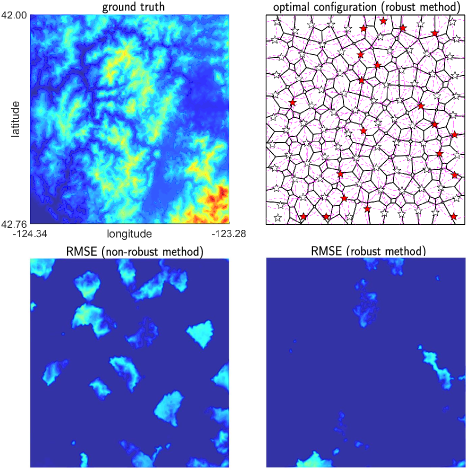
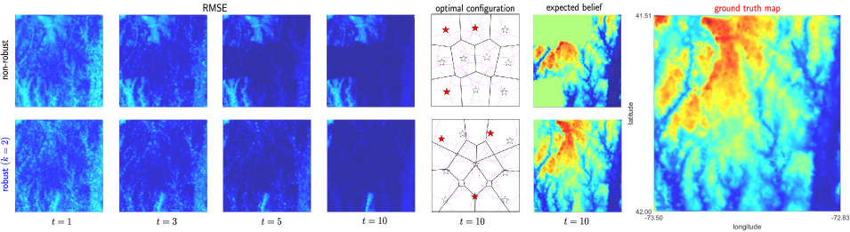
Simulation Settings: Let $\mathcal{Q}$ be a rectangular space $[42.00,41.51]\times[-73.49,-72.83]$ in $\mathbb{R}^{2}$ which corresponds to a mountainous region in Connecticut, U.S.A, where each coordinate corresponds to latitude and longitude, respectively. We let $\mathcal{I}=[-1000,\,4000]$ be a range of elevations in feet. Targets are uniformly distributed over $\mathcal{Q}$, and the ground truth target information over $\mathcal{Q}$ is depicted in Fig. 4 (right). The robots have no prior knowledge of the target information. A number of particles used for the SIR filter is $N=N_{1}\times N_{2}=5000\times 100$. We consider Gaussian distribution to for both the perception and the detection model. Each sensor’s measurement noise covariance matrix is $\Sigma_{I}=0.5\mathbf{I}$, and the binary detector’s noise covariance matrix is $\Sigma_{B}=0.04\mathbf{I}$ where $\mathbf{I}\in\mathbb{R}^{d\times d}$ is an identity matrix. In our simulation, we compare the three methods summarized in Table I.

TABLE I: Summary of deployment methods considered in current section.

algorithm type:	gradient computation	related studies
non-robust	fully decentralized	[3, 10, 11]
robust ($k=2$)	decentralized	current paper
max. information gain	centralized	[1, 2, 4, 5, 6]

Figure 2: An illustration of the convergence of two different deployment strategies, top: non-robust, bottom: robust ($k=2$) (stars: positions of robots, polygons: partition).

(a)

(b)

Figure 3: (a) convergence test for one-time deployment with different methods, (b) comparison of K-L divergence values between different methods.

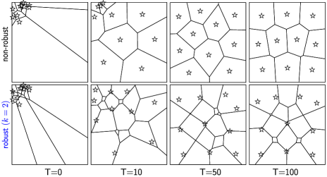
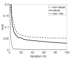
Convergence of Our Deployment Strategy: First, the behavior of the deployment strategy is discussed. Given a uniform initial prior belief and an initial configuration at $t=0$ (Fig. 2 (top-left)), three algorithms, summarized in Table I, were tested. Fig. 2 shows positions of robots after the $T$ number of iterations with (a) the non-robust method and (b) robust method ($k=2$). Fig. 3(a) compares the convergence speeds between the three methods. The cost on the $y$-axis corresponds to the probability of missed detection. Notice that the maximum information algorithm has a lower cost, but it relies on a centralized scheme that is typically impossible to realize in practice.

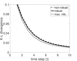
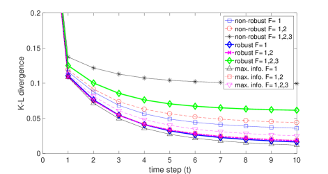
Environmental Mapping/Filtering Performance Without Sensor Failure: Next, we present the evolution of the belief to build an estimate of the elevation map after the deployment strategy has been completed. Fig. 3(b) compares the K-L divergence values between the different strategies during the filtering process. While the maximum information gain approach shows the best result, the robust deployment strategy has competitive mapping performance relative to the ground truth despite being a decentralized approach.

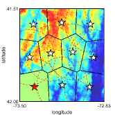
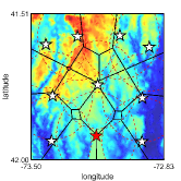
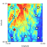
Robustness to Sensor Failure: We next present several examples with varying numbers of sensor failures wherein the robust method clearly illustrates appealing behavior when compared to its less robust counterparts. In this experiment, the number of sensor failures was varied by $\mathcal{F}\in\{\{1\},\,\{1,2\},\,\{1,2,3\}\}$. Results for robots configuration and target distributions after the $10^{\textup{th}}$ step with the non-robust, robust, and maximum information methods in the case when $\mathcal{F}=\{1\}$ are shown in Fig. 5. Fig. 4 shows the time evolutions of root-mean-square error (RMSE) between constructed map and the ground truth map for the non-robust (top) and robust (bottom) methods when $\mathcal{F}=\{1,2,3\}$. Fig. 6 compares the K-L divergence between different methods when $\left|\mathcal{F}\right|$ was varied between $1$ and $3$. As can be seen from Fig 5–6, the map retrieved by the proposed method when $k=2$ is consistently more robust to sensor failure when compared to existing methods. Note in Fig 5 (middle and right) the unmapped area is due to the limited sensing range.

Figure 4: An illustration of the time evolution of the root-mean-square error (RMSE) (in ft) between the constructed map and the ground truth map for non-robust method (top) and robust method (bottom) where 3 nodes have randomly failed (left 4 images). An illustration of the robot deployment (depicted with stars, where the red stars are failed sensors) sensor footprint (dashed lines), and partition (polygons) for the non-robust (top) and robust method (bottom) is also shown (5th column). The computed expected belief is also depicted from the non-robust (top) and robust (bottom) methods (6th column) and the ground truth image is depicted (right). The colormap is using MATLAB’s jet colormap.

Figure 5: The expected beliefs at $t=10$ from the non-robust method (left), robust method (middle), and max. information gain method (right) along with robot configurations (stars are robot locations and red stars are robots whose sensors have failed), footprints (dashed line), and partition (polygons) is depicted. The ground truth elevation map is on the right of Fig. 4. The colormap is using MATLAB’s jet colormap.

Figure 6: Comparison of K-L divergence of the ground truth distribution between different methods during belief propagation when a component of the nodes have failed.

Statistical Results with Varying Initial Conditions and Fault Compositions: Statistical results shows that our method can be used to estimate an arbitrary target distribution given a randomly chosen initial configuration, with different fault compositions well. Fig. 7 shows a distribution of K-L divergence values at $t=10$ for $100$ test examples consisting of random initial configurations with uniformly sampled number of faults between $1$ and $5$ with $10$ robots.

Figure 7: Comparison of robustness between different methods on $100$ randomly generated tests at $t=10$.

Scalability of our Method: Fig. 3 shows an example with $100$ robots (with $20$ sensors failures) where the robust method outperforms the non-robust method. This is due to the presence of central information fusion server which requires a full communication throughout the MSN. This is typically infeasible in real-world applications.

VII Conclusions and Future Work

This paper presents a deployment strategy for a mobile sensor network to enable the recovery of an environmental map over a bounded space in a manner that is robust to sensor failures. We plan to employ multi-agent patrolling [25, 12] or sweep coverage [26] to resolve problems associated with not having enough sensors to fully cover a target space. Also, as reported in the literature [16], our combined sensor model has been adopted to emulate the real-world laser scanner’s behavior; nevertheless, we plan to conduct extensive real world multi-robot experiments for further validation of our range sensor model.

References

- [1] D. Connor, P. Martin, and T. Scott, “Airborne radiation mapping: overview and application of current and future aerial systems,” International Journal of Remote Sensing, vol. 37, no. 24, pp. 5953–5987, 2016.
- [2] M. Schwager, P. Dames, D. Rus, and V. Kumar, “A multi-robot control policy for information gathering in the presence of unknown hazards,” in Robotics Research. Springer, 2017, pp. 455–472.
- [3] R. A. Cortez, H. G. Tanner, R. Lumia, and C. T. Abdallah, “Information surfing for radiation map building,” International Journal of Robotics and Automation, vol. 26, no. 1, p. 4, 2011.
- [4] C. D. Pahlajani, I. Poulakakis, and H. G. Tanner, “Networked decision making for poisson processes with applications to nuclear detection,” IEEE Transactions on Automatic Control, vol. 59, no. 1, pp. 193–198, 2014.
- [5] B. J. Julian, M. Angermann, M. Schwager, and D. Rus, “Distributed robotic sensor networks: An information-theoretic approach,” The International Journal of Robotics Research, vol. 31, no. 10, pp. 1134–1154, 2012.
- [6] K. M. Lynch, I. B. Schwartz, P. Yang, and R. A. Freeman, “Decentralized environmental modeling by mobile sensor networks,” IEEE Transactions on Robotics, vol. 24, no. 3, pp. 710–724, 2008.
- [7] J. A. Hoffman, J. R. Cunningham, A. J. Suleh, A. Sundsmo, D. Dekker, F. Vago, K. Munly, E. K. Igonya, and J. Hunt-Glassman, “Mobile direct observation treatment for tuberculosis patients: a technical feasibility pilot using mobile phones in nairobi, kenya,” American journal of preventive medicine, vol. 39, no. 1, pp. 78–80, 2010.
- [8] P. Yang, R. A. Freeman, G. J. Gordon, K. M. Lynch, S. S. Srinivasa, and R. Sukthankar, “Decentralized estimation and control of graph connectivity for mobile sensor networks,” Automatica, vol. 46, no. 2, pp. 390–396, 2010.
- [9] M. I. Shamos and D. Hoey, “Closest-point problems,” in Foundations of Computer Science, 1975., 16th Annual Symposium on. IEEE, 1975, pp. 151–162.
- [10] S. Bandyopadhyay and E. J. Coyle, “An energy efficient hierarchical clustering algorithm for wireless sensor networks,” in INFOCOM 2003. 23nd Annual Joint Conference of the IEEE Computer and Communications., vol. 3. IEEE, 2003, pp. 1713–1723.
- [11] T. Patten, R. Fitch, and S. Sukkarieh, “Large-scale near-optimal decentralised information gathering with multiple mobile robots,” in Proceedings of Australasian Conference on Robotics and Automation, 2013.
- [12] S. Kemna, J. G. Rogers, C. Nieto-Granda, S. Young, and G. S. Sukhatme, “Multi-robot coordination through dynamic voronoi partitioning for informative adaptive sampling in communication-constrained environments,” in Robotics and Automation (ICRA), 2017 IEEE International Conference on. IEEE, 2017, pp. 2124–2130.
- [13] S. Hutchinson and T. Bretl, “Robust optimal deployment of mobile sensor networks,” in Robotics and Automation (ICRA), 2012 IEEE International Conference on, 2012, p. 671–676.
- [14] R. Viswanathan and P. K. Varshney, “Distributed detection with multiple sensors part i. fundamentals,” Proceedings of the IEEE, vol. 85, no. 1, pp. 54–63, 1997.
- [15] P. M. Djuric, M. Vemula, and M. F. Bugallo, “Target tracking by particle filtering in binary sensor networks,” IEEE Transactions on Signal Processing, vol. 56, no. 6, pp. 2229–2238, 2008.
- [16] D. Anguelov, D. Koller, E. Parker, and S. Thrun, “Detecting and modeling doors with mobile robots,” in Robotics and Automation, 2004. Proceedings. ICRA’04. 2004 IEEE International Conference on, vol. 4. IEEE, 2004, pp. 3777–3784.
- [17] A. W. Stroupe, M. C. Martin, and T. Balch, “Distributed sensor fusion for object position estimation by multi-robot systems,” in Robotics and Automation, 2001. Proceedings 2001 ICRA. IEEE International Conference on, vol. 2. IEEE, 2001, pp. 1092–1098.
- [18] J. Cortés, S. Martínez, T. Karatas, and F. Bullo, “Coverage control for mobile sensing networks,” Robotics and Automation, IEEE Transactions on, vol. 20, no. 2, p. 243–255, 2004.
- [19] H. Park and S. Hutchinson, “Robust optimal deployment in mobile sensor networks with peer-to-peer communication,” in Robotics and Automation (ICRA), 2014 IEEE International Conference on. IEEE, 2014, pp. 2144–2149.
- [20] S. Kumar, T. H. Lai, and J. Balogh, “On k-coverage in a mostly sleeping sensor network,” in Proceedings of the 10th annual international conference on Mobile computing and networking. ACM, 2004, pp. 144–158.
- [21] D.-T. Lee, “On k-nearest neighbor voronoi diagrams in the plane,” IEEE Trans. Computers, vol. 31, no. 6, pp. 478–487, 1982.
- [22] S. M. LaValle, Planning algorithms. Cambridge university press, 2006.
- [23] D. Crisan and A. Doucet, “A survey of convergence results on particle filtering methods for practitioners,” IEEE Transactions on signal processing, vol. 50, no. 3, pp. 736–746, 2002.
- [24] H. M. Choset, Principles of robot motion: theory, algorithms, and implementation. MIT press, 2005.
- [25] D. Portugal and R. Rocha, “A survey on multi-robot patrolling algorithms,” in Doctoral Conference on Computing, Electrical and Industrial Systems. Springer, 2011, pp. 139–146.
- [26] I. Rekleitis, V. Lee-Shue, A. P. New, and H. Choset, “Limited communication, multi-robot team based coverage,” in Robotics and Automation, 2004. Proceedings. ICRA’04. 2004 IEEE International Conference on, vol. 4. IEEE, 2004, pp. 3462–3468.