A matrix analysis approach to discrete comparison principles for nonmonotone PDE

Abstract.

We consider a linear algebra approach to establishing a discrete comparison principle for a nonmonotone class of quasilinear elliptic partial differential equations. In the absence of a lower order term, we require local conditions on the mesh to establish the comparison principle and uniqueness of the piecewise linear finite element solution. We consider the assembled matrix corresponding to the linearized problem satisfied by the difference of two solutions to the nonlinear problem. Monotonicity of the assembled matrix establishes a maximum principle for the linear problem and a comparison principle for the nonlinear problem. The matrix analysis approach to the discrete comparison principle yields sharper constants and more relaxed mesh conditions than does the argument by contradiction used in previous work.

1. Introduction

We consider a linear algebra approach to develop a discrete comparison principle for the equation

$$-{\operatorname{div}}(\kappa(x,u)\nabla u)+g(x,u)=f,\text{ in }\Omega\subset{\mathbb{R}}^{2},$$ (1.1)

with homogeneous Dirichlet conditions

$$u=0\text{ on }\Gamma_{D}=\partial\Omega.$$ (1.2)

The discrete comparison principle directly implies uniqueness of the discrete solution, in agreement with the comparison principle and uniqueness for the continuous problem.

The PDE (1.1) is both nonmonotone and nonvariational (see, e.g., [12]); and, as demonstrated in [2], uniqueness of solutions to its finite element approximation can fail if the mesh is too coarse, even where the PDE solution is known to be unique. Asympototic error estimates for a finite element approximation as the meshsize $h\rightarrow 0$ were first shown in 1975 in [7]. More recently, similar results were shown to hold under integration by quadrature in [1]. In [2], an argument by contradiction related to the approach used in the continuous case is used to establish a discrete comparison principle based on the condition that the mesh partition is globally fine enough. The current authors used similar ideas in [14, 15] to demonstrate that a local verifiable condition based on the variance of the solution over each element, rather than a global meshize condition, is sufficient for uniqueness of solutions in the absence of a lower order term. Here, we improve the constant appearing in the condition and also relax the angle condition on the mesh.

This manuscript is motivated by the linear algebra approach used to establish a discrete maximum principle in [4], demonstrated to improve previously established constants. The current authors also showed in [14] that the maximum principle for the linear reaction-diffusion equation developed in [4, Theorem 3.8] has a direct application to a discrete comparison principle for the semilinear problem, $-\Delta u+g(x,u)=f$; and, the matrix analysis approach yields an improved constant. Here, we extend the analysis to quasilinear problems. In the semilinear case, the argument follows by showing that the assembled matrix in question is a Stieltjes matrix, which is a symmetric positive definite matrix with nonpositive off-diagonal entries. The particulars of the analysis do not apply in the quasilinear case, as the corresponding coefficient matrix for the linearization of (1.1) is easily seen to be nonsymmetric, hence not Stieltjes.

In this paper, we develop conditions under which the assembled coefficient matrix $A$ corresponding to the PDE satisfied by the difference between a subsolution and supersolution of (1.1) is monotone. We proceed by first showing it is a $Z$-matrix, one with nonpositive off-diagonal entries; then, showing there is a diagonal matrix $D$ such that $AD$ is strictly diagonally dominant, satisfying a condition for monotonicity found in [10, 13]. The first main contribution of this work is improving the constants in the local condition for the discrete comparison principle hence uniqueness to hold. The second main contribution is establishing the discrete comparison principle holds for problem (1.1) on meshes with at least some right angles.

In previous work by the authors [14, 15], the mesh was assumed acute, meaning all interior angles were bounded below $\pi/2$. In the current results, interior angles can be no greater than $\pi/2$, and opposite angles across each edge must sum to less that $\pi$. It is well known (see, for instance [19, Lemma 2.1]), that for the assembled matrix for the Laplacian, monotonicity holds under the condition that the mesh is Delaunay, meaning the angles opposite each edge sum to no more than $\pi$. More general geometric conditions for a discrete maximum principle for Poisson’s equation are developed in [9], in which certain refinements of meshes satisfying monotonicity conditions are shown to remain monotone. The stronger condition on the geometry in this work comes from the variable-dependence in the principal part of the linearized problem, so that improved conditions for Laplace operators do not directly apply.

The theory of monotone matrices in numerical analysis has been well-studied, largely with respect to the convergence of iterative methods [17, 20]. In [13], a collection of 40 conditions for a $Z$-matrix to be a nonsingular $M$-matrix, hence monotone, is drawn from the literature. We use one of those conditions, which appears earlier in [10], to establish our results. The main technical challenge of this work is to understand the monotonicity of the coefficient matrix arising from the discretization of a linear convection-diffusion, or reaction-convection-diffusion equation. This matrix is nonsymmetric, and lacks strict diagonal dominance. The failure in the linear case for a convection-diffusion coefficient matrix to have strictly positive row-sums is also discussed in [19].

The comparison principle for (1.1) is equivalent to a maximum principle for a linearized equation satisfied by the difference of a subsolution and supersolution to (1.1), which is demonstrated here by the monotonicity of the assembled coefficient matrix. This relationship and its implication for the uniqueness of the finite element solution is summarized in Theorem 3.3.

The remainder of the paper is structured as follows. In Section 2, the discretization and discrete comparison principle are introduced. Then, the linearized problem used to investigate the comparison principle is derived. Theorem 3.3 summarizes the relationship between the monotonicity of the assembled matrix for the linearized problem and the comparison principle for the nonlinear problem. The definitions of $Z$, $L$ and $M$ matrices, and the relevant theorems on their relationships are recalled from the literature. Section 4 contains the technical estimates used to show the assembled matrix $A$ is monotone.

2. Preliminaries

We make the following assumptions on the problem data $\kappa(\cdot\,,\cdot)$ and $g(\cdot\,,\cdot)$.

Assumption 2.1.

Assume $\kappa(x,\eta)$ and $g(x,\eta)$ are Carathéodory functions, measurable in $x$ for each $\eta\in{\mathbb{R}}$, and $C^{1}$ in $\eta$ for $\text{a.e.\,}x\in\Omega$. Assume there are constants $0<k_{\alpha}<k_{\beta}$ with

$$k_{\alpha}\leq\kappa(x,\eta)\leq k_{\beta},$$ (2.1)

for all $\eta\in{\mathbb{R}}$, and $\text{a.e.\,}x\in\Omega$. Assume there is a positive $K_{\eta}$ with

$$\left|\frac{\partial\kappa}{\partial\eta}(x,\eta)\right|\leq K_{\eta},$$ (2.2)

for all $\eta\in{\mathbb{R}}$ and $\text{a.e.\,}x\in\Omega$. Assume $g(x,\eta)$ is nondecreasing with respect to its second argument, and there is a constant $G_{\eta}$ with

$$0\leq\frac{\partial g}{\partial\eta}(x,\eta)\leq G_{\eta},$$ (2.3)

for all $\eta\in{\mathbb{R}}$ and $\text{a.e.\,}x\in\Omega$.

Under Assumption 2.1, the PDE is known to satisfy a comparison principle and have a unique solution, as demonstrated in [8, 16] and [11, Chapter 10]. Additionally, the weak form of (1.1) is given as follows for $V=H_{0}^{1}(\Omega)$, the closed subspace of $H^{1}$ with vanishing trace on $\partial\Omega$. Find $u\in V$ such that

$$\int_{\Omega}\kappa(x,u)\nabla u\!\cdot\!\nabla v+g(x,u)v\,{\operatorname{d}}x=\int_{\Omega}fv\,{\operatorname{d}}x,\text{ for all }v\in V.$$ (2.4)

The functional setting of the weak form can be understood in the context of the Leray-Lions conditions for pseudomonotonicity. We refer interested readers to [5, Chapter 2-3] for further details. We note that the class of problems defined by the assumptions in this section is called nonmonotone because the inequality

$$\int_{\Omega}(\kappa(x,w)\nabla w-\kappa(x,v)\nabla v)\!\cdot\!\nabla(w-v)\,{\operatorname{d}}x\geq 0,$$

does not in general hold for all $w,v\in V$, even for $\kappa=\kappa(u)$, with $\kappa^{\prime}(u)\geq 0$.

2.1. Discretization

Let ${\mathcal{T}}$ be a conforming simplicial partition of domain $\Omega$ that exactly captures the boundary. Let $\overline{\mathcal{Q}}$ be the collection of vertices or nodes of ${\mathcal{T}}$, and let ${\mathcal{Q}}=\overline{\mathcal{Q}}\setminus\partial\Omega$ be the set nodes that do not lie on the Dirichlet boundary, corresponding to the mesh degrees of freedom. Let ${\mathcal{V}}\subsetneq V$ be the discrete space spanned by the piecewise linear basis functions $\{\varphi_{j}\}$ that satisfy $\varphi_{i}(q_{i})=1$ and $\varphi_{i}(q_{j})=0$ for each $q_{j}\in\overline{\mathcal{Q}}$ with $q_{j}\neq q_{i}$. Define the non-negative subset of ${\mathcal{V}}$ by ${\mathcal{V}}^{+}\coloneqq\{v\in{\mathcal{V}}~{}\big{|}~{}v\geq 0\}$.

Let $\omega_{i}$ be the support of the basis function $\varphi_{i}$. Define the intersection of support for any two basis functions with respect to a global numbering by $\omega_{ij}=\omega_{i}\cap\omega_{j}$. In terms of the corresponding nodes $q_{i}$ and $q_{j}$, it follows that $\omega_{ij}$ is the union of elements that share both $q_{i}$ and $q_{j}$ as vertices.

$$\omega_{ij}=\bigcup\{T\in{\mathcal{T}}~{}\big{|}~{}q_{i}\in T~{}\text{ and }q_{j}\in T\}.$$

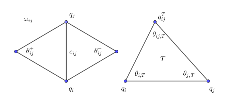
Additional notation for the discretization is summarized as follows, and illustrated in Figure 1.

• $e_{ij}$, denotes the edge connecting vertices $q_{i}$ and $q_{j}$.

• $\theta_{ij}^{+}$ and $\theta_{ij}^{-}$ denote the two respective angles opposite edge $e_{ij}$ in $\omega_{ij}$.

• $\theta_{j,T}$ denotes the interior angle of triangle $T$ at vertex $q_{j}$, and $\theta_{ij,T}$ denotes the interior angle opposite vertices $q_{i}$ and $q_{j}$ in triangle $T$.

• $q_{ij}^{T}$ denotes the vertex opposite both $q_{i}$ and $q_{j}$ in triangle $T$.

• $\varphi_{ij}^{T}$ denotes the basis function associated with $q_{ij}^{T}$ in triangle $T$.

• $\delta^{e}_{ij}(v)=|v(q_{i})-v(q_{j})|$ is the absolute difference of nodal values over edge $e_{ij}$.

• $\delta_{\omega}^{(i)}(v)=\max\{\delta_{jk}^{e}(v)~{}\big{|}~{}q_{j},q_{k}\in\omega,~{}j,k\neq i\}$ is the maximum difference between neighboring nodal values of $v$ in $\omega$, over each edge not touching vertex $q_{i}$.

• $\delta_{\omega}(v)=\max\{\delta_{jk}^{e}(v)~{}\big{|}~{}q_{j},q_{k}\in\omega\}$ denotes the maximum difference between neighboring nodal values of $v$ in $\omega$.

• $|T|$ denotes the area of triangle $T\in{\mathcal{T}}$.

• $|T_{\mathcal{T}}|=\max_{T\in{\mathcal{T}}}|T|$.

• $\overline{\mathcal{Q}}_{i}=\{q_{j}\in\overline{\mathcal{Q}}~{}\big{|}~{}q_{j}\in\omega_{i},~{}j\neq i\}$, denotes the set of vertices neighboring $q_{i}$, including those on $\Gamma_{D}$.

• ${\mathcal{Q}}_{i}=\overline{\mathcal{Q}}_{i}\setminus\Gamma_{D}$, the set of non-Dirichlet vertices neighboring $q_{i}$.

Figure 1. Left: Schematic of a patch. Right: Schematic of an element.

Assumption 2.2.

It is assumed any interior angle of the mesh satisfies $\theta\leq\pi/2$, and that any two angles opposite an edge must sum to less than $\pi$. In particular, there is a constant $\beta_{m}>0$ for which

$$\cot\theta_{ij}^{+}+\cot\theta_{ij}^{-}>\beta_{m},~{}\text{ for each }~{}\omega_{ij}\subset{\mathcal{T}}.$$ (2.5)

It is also assumed that the mesh satisfies a smallest-angle condition over each neighborhood $\omega_{ij}$. There is a constant $\beta_{M}>0$ for which

$$\cot\theta_{ij}^{+}+\cot\theta_{ij}^{-}+\sum_{T\in\omega_{ij}}\cot\theta_{i,T}\leq\beta_{M}~{}\text{ for each }~{}\omega_{ij}\subset{\mathcal{T}}.$$ (2.6)

2.2. Comparison framework

Consider the problems: Find $u_{i}\subset{\mathcal{V}}$ such that

$$\int_{\Omega}\kappa(x,u_{i})\nabla u_{i}\!\cdot\!\nabla v+g(x,u_{i})v\,{\operatorname{d}}x=\int_{\Omega}f_{i}v\,{\operatorname{d}}x,\text{ for all }v\in{\mathcal{V}},$$ (2.7)

for $f_{i}\in L_{2}(\Omega)$, $i=1,2$. The discrete comparison principle for (2.7) states that whenever $f_{1}\leq f_{2}$, ($\text{a.e.\,}x\in\Omega$), meaning $\int_{\Omega}(f_{1}-f_{2})v\,{\operatorname{d}}x\leq 0$, for each $v\in{\mathcal{V}}^{+}$, then it holds that $u_{1}\leq u_{2}$.

The comparison principle can be restated in terms of a maximum principle for $w=u_{1}-u_{2}$. The discrete problem satisfied by $w$ can be understood by applying Taylor’s theorem to the difference of (2.7) with $i=1$ and $i=2$.

$$\int_{\Omega}\left(\kappa(x,u_{1})\nabla u_{1}\!\cdot\!\nabla v+g(x,u_{1})v\right)\,{\operatorname{d}}x-\int_{\Omega}\left(\kappa(x,u_{2})\nabla u_{2}\!\cdot\!\nabla v+g(x,u_{2})v\right)\,{\operatorname{d}}x$$

$$=\int_{\Omega}\kappa(x,u_{1})\nabla(u_{1}-u_{2})\!\cdot\!\nabla v-(\kappa(x,u_{2})-\kappa(x,u_{1}))\nabla u_{2}\!\cdot\!\nabla v\,{\operatorname{d}}x$$

$$+\int_{\Omega}(g(x,u_{1})-g(x,u_{2}))v\,{\operatorname{d}}x$$

$$=\int_{\Omega}\kappa(x,u_{1})\nabla(u_{1}-u_{2})\!\cdot\!\nabla v\,{\operatorname{d}}x-\int_{\Omega}\left(\int_{0}^{1}\frac{\partial\kappa}{\partial\eta}(x,z(t))(u_{1}-u_{2})\,dt\right)\nabla u_{2}\!\cdot\!\nabla v\,{\operatorname{d}}x$$

$$+\int_{\Omega}\left(\int_{0}^{1}\frac{\partial g}{\partial\eta}(x,z(t))(u_{1}-u_{2})\,dt\right)v\,{\operatorname{d}}x,$$ (2.8)

where $z(t)=tu_{1}+(1-t)u_{2}$, for $0\leq t\leq 1$. Letting $w=u_{1}-u_{2}$, the equation satisfied by $w$ is then

$$\int_{\Omega}\kappa(x,u_{1})\nabla w\!\cdot\!\nabla v\,{\operatorname{d}}x+\int_{\Omega}\left(\int_{0}^{1}\frac{\partial\kappa}{\partial\eta}(x,z(t))\,dt\right)w\nabla u_{2}\!\cdot\!\nabla v\,{\operatorname{d}}x$$

$$+\int_{\Omega}\left(\int_{0}^{1}\frac{\partial g}{\partial\eta}(x,z(t))w\,dt\right)v\,{\operatorname{d}}x=\int_{\Omega}(f_{1}-f_{2})v\,{\operatorname{d}}x,~{}\text{ for all }v\in{\mathcal{V}}.$$ (2.9)

The comparison principle for $u_{1}$ and $u_{2}$ in (2.7) is then equivalent to the weak maximum principle for $w=u_{1}-u_{2}$ in (2.2), namely $w\leq 0$ whenenever $f_{1}-f_{2}\leq 0$. We now turn our attention to establishing the weak maximum principle for $w$.

3. Discrete maximum principle

From (2.2), the linear equation for $w$ is a general second order elliptic equation with convection and reaction terms

$$\int_{\Omega}\kappa(x,u_{1})\nabla w\cdot\nabla v\,{\operatorname{d}}x+\int_{\Omega}\vec{b}(x,u_{2})w\!\cdot\!\nabla v\,{\operatorname{d}}x+\int_{\Omega}c(x)wv\,{\operatorname{d}}x=\int_{\Omega}(f_{1}-f_{2})v\,{\operatorname{d}}x,$$ (3.1)

for all $v\in{\mathcal{V}}$, with

$$\vec{b}(x) \coloneqq b(x)\nabla u_{2}(x),~{}\text{ with }~{}b(x)\coloneqq\int_{0}^{1}\frac{\partial\kappa}{\partial\eta}(x,z(t))\,{\operatorname{d}}t,$$ (3.2)

$$c(x) \coloneqq\int_{0}^{1}\frac{\partial g}{\partial\eta}(x,z(t))\,{\operatorname{d}}t.$$ (3.3)

We now turn our attention to the properties of the assembled system (3.1)-(3.3). The discrete function $w\in{\mathcal{V}}$ has the expansion in basis functions $w=\sum_{j=1}^{n}W_{j}\varphi_{j}$, where $n$ is the number of mesh degrees of freedom. Choosing the test functions $v=\varphi_{i}$ for each $i=1,\cdots,n$ in Equation (3.1), we obtain the equivalent matrix problem $AW=F$. In particular, $W=(W_{1},\cdots,W_{n})^{T}$, $F=(F_{1},\cdots,F_{n})^{T}$ with $A=(a_{ij})$ and $F_{i}$ defined entrywise by

$$a_{ij} =\int_{\omega_{ij}}\kappa(x,u_{1})\nabla\varphi_{j}\!\cdot\!\nabla\varphi_{i}\,{\operatorname{d}}x+\int_{\omega_{ij}}\vec{b}(x,u_{2})\varphi_{j}\!\cdot\!\nabla\varphi_{i}\,{\operatorname{d}}x+\int_{\omega_{ij}}c(x)\varphi_{j}\varphi_{i}\,{\operatorname{d}}x$$ (3.4)

$$F_{i} =\int_{\omega_{i}}(f_{1}-f_{2})\varphi_{i}\,{\operatorname{d}}x.$$ (3.5)

We now investigate the maximum principle for $w$ through the monotonicity of matrix $A$ given by (3.4).

Definition 3.1 (Monotone matrix).

A real square matrix $A$ is monotone (in the sense of [6, Section 23] ) if for all real vectors $v$, $Av\geq 0$ implies $v\geq 0$, where $\geq$ is the element-wise ordering.

By this definition, a monotone matrix is nonsingular because if $A$ is a monotone matrix and $x$ is a vector in its nullspace, then both $x\geq 0$ and $-x\geq 0$, implying $x=0$. We mention another relevant property of monotone matrices.

Proposition 3.2.

$A$ is monotone iff $A$ is invertible and $A^{-1}\geq 0$.

Proof.

If $A$ is monotone, then $A$ is nonsingular and $A^{-1}$ exists. Let $x$ be the $i$th column of $A^{-1}$, so we have $Ax=e_{i}$, the $i$-th standard basis vector. This shows $Ax\geq 0$ which implies $x\geq 0.$ Therefore $A^{-1}\geq 0.$

Reversely, suppose $A$ has an inverse and $A^{-1}\geq 0.$ If $Ax\geq 0$, then $x=A^{-1}Ax\geq A^{-1}0=0.$ Hence $A$ is monotone. ∎

The next theorem summarizes how monotonicity of the assembled matrix for $w$ implies the comparison principle, hence uniqueness of the solution.

Theorem 3.3.

Suppose the functions $\kappa(x,\eta)$ and $g(x,\eta)$ are each measurable with respect to the first argument, and $C^{1}$ with respect to the second. Let $u_{i}\subset{\mathcal{V}}$ solve

$$\int_{\Omega}\kappa(x,u_{i})\nabla u_{i}\!\cdot\!\nabla v+g(x,u_{i})v\,{\operatorname{d}}x=\int_{\Omega}f_{i}v\,{\operatorname{d}}x,\text{ for all }v\in{\mathcal{V}},$$ (3.6)

for $f_{i}\in L_{2}(\Omega)$, $i=1,2$, with $\int_{\Omega}(f_{1}-f_{2})v\,{\operatorname{d}}x\leq 0$, for all $v\in{\mathcal{V}}^{+}$. Let $A$ be the coefficient matrix defined by (3.4), and $F$ the vector defined by (3.5). Then if $A$ is monotone, $u_{1}\leq u_{2}$. Moreover, if $f_{1}=f_{2}$, then $u_{1}=u_{2}$.

Proof.

Let the discrete function $w\in{\mathcal{V}}$ be given by $w=\sum_{j=1}^{n}W_{j}\varphi_{j}$, with $W=(W_{1},\cdots,W_{n})^{T}$, where $n=\text{card}({\mathcal{Q}})$, the number of mesh degrees of freedom. The monotonicity of $A$ implies its invertibility. By equations (2.2)-(2.2), and the definitions of $A$ and $F$, the vector $W$ that solves $AW=F$ uniquely defines $w\in{\mathcal{V}}$ that satisfies $w=u_{1}-u_{2}$.

Since $A$ is monotone, $F\leq 0$ implies $W\leq 0$ which by the nonnegativity of basis functions implies $w\leq 0$ implying $u_{1}\leq u_{2}$. If $f_{1}=f_{2}$, it follows that $u_{1}=u_{2}$. ∎

Remark 3.4.

The monotonicity of matrix $A$ given by (3.4) also, by the reasoning above, establishes a discrete maximum principle for the linear problem (3.1).

In the remainder of the paper we develop conditions under which the assembled matrix (3.4) is monotone. Three related classes of matrices we enounter in the proof are $Z$-matrices, $L$-matrices and $M$-matrices, defined as follows.

Definition 3.5 ($Z$-matrix).

A matrix $A$ is called an $Z$-matrix if $a_{ij}\leq 0$ when $i\neq j$ (see [10, Definition 4,1],[13]).

A $Z$-matrix with positive diagonal entries is also called an $L$-matrix.

Definition 3.6 ($L$-matrix).

A matrix $A$ is called an $L$-matrix if $a_{ii}>0$ for all $i$ , and $a_{ij}\leq 0$ when $i\neq j$ (see [18, Definition 2.9], [20, Chapter 2, Definition 7.1])

A monotone $Z$-matrix is an $M$-matrix.

Definition 3.7 ($M$-matrix, see [17, Definition 3.22]).

A real $n\times n$ matrix $A=(a_{ij})$ with $a_{ij}\leq 0$ for all $i\neq j$ is an $M$-matrix if $A$ is nonsingular and $A^{-1}\geq 0$.

We note the equivalence of this definition to [20, Definition 7.3], and to a nonsingular $M$-matrix, as in [13]. If the off-diagonal entries of $A$ are nonpositive, then $A$ is monotone if and only if $A$ is an $M$-matrix. This is clear from the Proposition 3.2 of the monotone matrix, and the definition of the $M$-matrix.

In what follows, we will show the monotonicity of the coefficient matrix $A$ given by (3.4), by first showing $A$ is a $Z$-matrix: the off-diagonal entries are nonpositive; then showing it is monotone, by the following 1962 result of M. Fiedler and V. Pták. We first recall the standard definition of (strict) diagonal dominance.

Definition 3.8.

An $n\times n$ matrix is strictly diagonally dominant if

$$|a_{ii}|>\sum_{j=1,j\neq i}^{n}|a_{ij}|,~{}\text{ for all }~{}i=1,\ldots,n.$$ (3.7)

Strict diagonal dominance may also be called strong diagonal dominance [20, p.41]. A matrix is called diagonally dominant (or weakly diagonally dominant) if equality is allowed in (3.7), with a strict inequality for at least one index $i$.

The full theorem of [10] presents 13 equivalent statements, here we paraphrase the two most relevant to our purposes.

Theorem 3.9.

[10, Theorem 4,3.4],[13, Theorem 1 (N39)] Let $A$ be a $Z$-matrix. Then $A$ is monotone if and only if there exists a diagonal matrix $D$ with positive diagonal elements such that the matrix $AD$ is strictly diagonally dominant.

Along the way to showing the monotonicity, we also show $A$ is an $L$-matrix: the diagonal entries are strictly positive. As as consequence of the monotonicity, $A$ is then also an $M$-matrix, as in the corresponding result of [13]. There are many characterizations of $Z$-matrices as $M$-matrices, as in the review paper [13], the references therein, and [17, Chapter 3]. Further discussion on the conditions relating $Z$-matrices, $L$-matrices and $M$-matrices may be found in [20, Chapter 2], and [18, Chapter 2]. For completeness, we also mention the results of F. Bouchon [3], which depend explicity on irreducibility properties of the assembled matrix. Referring to the counterexample of [9], the irreducibility can fail to hold in certain situations, even on a connected mesh. As the assembled matrix from (3.4) is not itself strictly diagonally dominant, and it is not obvious how to compute the spectral radius by direct means, we choose Theorem 3.9 as the simplest condition to demonstrate based on computationally verifiable conditions.

4. Properties of the assembled matrix

In this section, we develop conditions under which $A$, the coefficient matrix from (3.4), is a $Z$-matrix that satisfies Theorem 3.9, hence is monotone. Our main comparison result then follows from Theorem 3.3. Each entry $a_{ij}$ of matrix $A$ is given by (3.4) with $\vec{b}$ and $c$ given by (3.2) and (3.3), respectively. We now consider the conditions under which matrix $A$ has non-positive off-diagonal entries, meaning $A$ is a $Z$-matrix.

Lemma 4.1.

Let Assumption 2.1 and Assumption 2.2 hold. Let $A=(a_{ij})$ be given by (3.4). On satisfaction of the condition on the nodal values of $u_{2}$ and meshsize $|T_{\mathcal{T}}|$

$$\frac{1}{3\beta_{m}}\left\{K_{\eta}\beta_{M}\delta_{\omega_{ij}}(u_{2})+G_{\eta}|T_{\mathcal{T}}|\right\}\leq k_{\alpha},~{}\text{ for each }~{}\omega_{ij}\subset{\mathcal{T}},$$ (4.1)

it holds that $a_{ij}\leq 0$ for each $i\neq j$.

Proof.

Equivalently, and for convenience of later calculations, we consider the entry $a_{ji}$. By direct calculation, it holds for $i\neq j$ that.

$$\nabla\varphi_{i}\!\cdot\!\nabla\varphi_{j}\big{|}_{T}=\frac{-1}{2|T|}\cot\theta_{ij,T},$$ (4.2)

where $\theta_{ij,T}$ is the angle opposite edge $e_{ij}$ in triangle $T$. Equation (4.2) together with (2.1) and (2.5) implies

$$\int_{\omega_{ij}}\kappa(x,u_{1})\nabla\varphi_{i}\!\cdot\!\nabla\varphi_{j}\,{\operatorname{d}}x\leq k_{\alpha}\sum_{T\in\omega_{ij}}\int_{T}\nabla\varphi_{i}\!\cdot\!\nabla\varphi_{j}\,{\operatorname{d}}x=-\frac{k_{\alpha}}{2}(\cot\theta_{ij}^{+}+\cot\theta_{ij}^{-}),$$ (4.3)

for interior nodes, $q_{i},q_{j}\in{\mathcal{Q}}$. For the reaction term, $\int_{T}\varphi_{i}\varphi_{j}\,{\operatorname{d}}x={|T|}/{12}$. Together with (2.3) and (3.3), this implies

$$\int_{\omega_{ij}}c(x)\varphi_{i}\varphi_{j}\,{\operatorname{d}}x\leq\sum_{T\in\omega_{ij}}\frac{G_{\eta}|T|}{12},$$ (4.4)

for $q_{i},q_{j}\in{\mathcal{Q}}$.

To bound the nonsymmetric term, the following decomposition is useful. Over each triangle $T$ with vertices $q_{i},q_{i},q_{k}$ and discrete function $v\in{\mathcal{V}}$, we have

$$\nabla v=(v(q_{i})-v(q_{j}))\nabla\varphi_{i}+(v(q_{k})-v(q_{j}))\nabla\varphi_{k}.$$ (4.5)

Applying (4.2) and (4.5) with $v=u_{2}$ and $q_{k}=q_{ij}^{T}$ for each $T\in\omega_{ij}$ yields

$$\int_{\omega_{ij}}b(x)\nabla u_{2}\!\cdot\!\nabla\varphi_{j}\varphi_{i}\,{\operatorname{d}}x =(u_{2}(q_{i})-u_{2}(q_{j}))\int_{\omega_{ij}}\nabla\varphi_{i}\!\cdot\!\nabla\varphi_{j}\,b(x)\varphi_{i}\,{\operatorname{d}}x$$

$$+\sum_{T\in\omega_{ij}}(u_{2}(q_{ij}^{T})-u_{2}(q_{j}))\int_{T}\nabla\varphi_{ij}^{T}\!\cdot\!\nabla\varphi_{j}\,b(x)\varphi_{i}\,{\operatorname{d}}x$$

$$\leq\frac{K_{\eta}}{6}|u_{2}(q_{i})-u_{2}(q_{j})|(\cot\theta_{ij}^{+}+\cot\theta_{ij}^{-})$$

$$+\frac{K_{\eta}}{6}\sum_{T\in\omega_{ij}}|u_{2}(q_{ij}^{T})-u_{2}(q_{j})|\cot\theta_{i,T},$$ (4.6)

where the inequality follows from (2.2) of Assumption 2.1 and (3.2). For interior nodes $q_{i},q_{j}\in{\mathcal{Q}}$, we then have

$$\left|\int_{\omega_{ij}}\vec{b}(x)\!\cdot\!\nabla\varphi_{j}\varphi_{i}\,{\operatorname{d}}x\right|\leq\frac{K_{\eta}}{6}\left(\delta_{ij}^{e}(u_{2})(\cot\theta_{ij}^{+}+\cot\theta_{ij}^{-})+\delta_{\omega_{ij}}^{(i)}(u_{2})\sum_{T\in\omega_{ij}}\cot\theta_{i,T}\right).$$ (4.7)

Applying (4.3), (4.4) and (4.7) to (3.4), it holds for each $i,j$ for with $q_{i},q_{j}\in{\mathcal{Q}}$ that

$$a_{ji} \leq\frac{1}{2}\left(-k_{\alpha}+\frac{K_{\eta}}{3}\delta^{e}_{ij}(u_{2})\right)(\cot\theta_{ij}^{+}+\cot\theta_{ij}^{-})+\frac{1}{2}\sum_{T\in\omega_{ij}}\!\!\left(\frac{K_{\eta}}{3}\delta_{\omega_{ij}}^{(i)}(u_{2})\cot\theta_{i,T}+\frac{G_{\eta}|T|}{6}\right)$$

$$\leq\frac{1}{2}\left\{-k_{\alpha}\beta_{m}+\frac{K_{\eta}\beta_{M}}{3}\delta_{\omega_{ij}}(u_{2})+\frac{G_{\eta}|T_{\mathcal{T}}|}{3}\right\},$$ (4.8)

where the last inequality follows from the application of both angle conditions (2.5) and (2.6) from Assumption 2.2. If either $q_{i}$ or $q_{j}$ lies on the boundary $\partial\Omega$, then the contribution of each term is zero, and $a_{ij}=0$. The conclusion $a_{ij}\leq 0$ then follows under the condition (4.1). ∎

In the next lemma, we show the diagonal entries of $A$ are positive, under the given condition which bounds the difference of nodal values connecting each edge in the mesh. The local condition (4.9) for each $a_{ii}$ to be positive is weaker than (4.1), used above to determine the off-diagonal entries of $A$ are nonpositive, implying that matrix $A$ is an $L$-matrix as well as a $Z$-matrix.

Lemma 4.2.

Let Assumption 2.1 and Assumption 2.2 hold. Let $A=(a_{ij})$ be given by (3.4). Then under the condition

$$\delta_{ij}^{e}(u_{2})<\frac{3k_{\alpha}}{K_{\eta}},$$ (4.9)

it holds that $a_{ii}>0$, for each $i$.

Proof.

First consider the diffusion term. Summing integrals over each $\omega_{ij}\subset\omega_{i}$ integrates twice over $\omega_{i}$. Applying the identity $\nabla\varphi_{i}\!\cdot\!\nabla\varphi_{i}=-\nabla\varphi_{j}\!\cdot\!\nabla\varphi_{i}-\nabla\varphi_{ij}^{T}\!\cdot\!\nabla\varphi_{i}$, over each element $T\in\omega_{i}$ with nodal indices $q_{i},q_{j},q_{ij}^{T}$, and combining like terms to integrate each product once per element we have

$$\int_{\omega_{i}}\kappa(x,u_{1})\nabla\varphi_{i}\!\cdot\!\nabla\varphi_{i}\,{\operatorname{d}}x =\frac{1}{2}\sum_{\omega_{ij}\subset\omega_{i}}\int_{\omega_{ij}}\kappa(x,u_{1})\nabla\varphi_{i}\!\cdot\!\nabla\varphi_{i}\,{\operatorname{d}}x$$

$$=-\sum_{\omega_{ij}\subset\omega_{i}}\int_{\omega_{ij}}\kappa(x,u_{1})\nabla\varphi_{j}\!\cdot\!\nabla\varphi_{i}\,{\operatorname{d}}x$$

$$\geq\frac{k_{\alpha}}{2}\sum_{\omega_{ij}\subset\omega_{i}}(\cot\theta_{ij}^{-}+\cot\theta_{ij}^{+}),$$ (4.10)

where the last inequality follows from (2.1) and Assumption 2.2. Next, consider the nonsymmetric term. Summing integrals over each $\omega_{ij}\subset\omega_{i}$ then combining like terms as above we have

$$\int_{\omega_{i}}b(x)\nabla u_{2}\!\cdot\!\nabla\varphi_{i}\varphi_{i}\,{\operatorname{d}}x =\frac{1}{2}\sum_{\omega_{ij}\subset\omega_{i}}\int_{\omega_{ij}}b(x)\nabla u_{2}\!\cdot\!\nabla\varphi_{i}\varphi_{i}\,{\operatorname{d}}x$$

$$=\sum_{\omega_{ij}\subset\omega_{i}}(u_{2}(q_{j})-u_{2}(q_{i}))\int_{\omega_{ij}}\nabla\varphi_{j}\!\cdot\!\nabla\varphi_{i}b(x)\varphi_{i}\,{\operatorname{d}}x$$

$$\geq-\frac{K_{\eta}}{6}\sum_{\omega_{ij}\subset\omega_{i}}|u_{2}(q_{j})-u_{2}(q_{i})|(\cot\theta_{ij}^{+}+\cot\theta_{ij}^{-}),$$ (4.11)

where the last inequality follows from (2.2), Assumption 2.2, and the integration of $\varphi_{i}$ over each element. From (3.2) and (4) we have

$$\int_{\omega_{i}}\vec{b}(x)\!\cdot\!\nabla\varphi_{i}\varphi_{i}\,{\operatorname{d}}x\geq-\frac{K_{\eta}}{6}\sum_{\omega_{ij}\subset\omega}\delta_{ij}^{e}(u_{2})(\cot\theta_{ij}^{+}+\cot\theta_{ij}^{-}).$$ (4.12)

The lowest order term from (3.4) satisfies $\int_{\omega_{i}}c(x)\varphi_{i}^{2}\,{\operatorname{d}}x\geq 0,$ for $c(x)\geq 0$ as in (3.3) under the condition (2.3). Putting together (4) and (4.12) into (3.4), we have under Assumption 2.1

$$a_{ii} \geq\frac{1}{2}\sum_{\omega_{ij}\subset\omega_{i}}(\cot\theta_{ij}^{+}+\cot\theta_{ij}^{-})\left(-\frac{K_{\eta}}{3}\delta_{ij}^{e}(u_{2})+k_{\alpha}\right)$$

$$\geq\frac{\beta_{m}}{2}\left(-\frac{K_{\eta}}{3}\delta_{ij}^{e}(u_{2})+k_{\alpha}\right),$$ (4.13)

from which the result follows under condition (4.9). ∎

By the conditions of the previous two lemmas, and the computations of the next lemma, the matrx $A$ can be seen to have positive row-sums for each index $i$ such that vertex $q_{i}$ neighbors the Dirichlet boundary. In the next lemma, we constuct a diagonal matrix $D_{\varepsilon}^{\prime}$ for which the positivity of row-sums of $AD_{\varepsilon}^{\prime}$ is extended to indices $j$ such that $q_{j}$ neighbors a vertex which neighbors $\Gamma_{D}$. This is not sufficient to establish the comparison result which requires strict diagonal dominance of $AD$ for some $D$. However, it indicates how to construct a diagonal matrix $D$ with positive diagonal entries such that the positivity of row-sums of $AD$ can be extended to rows corresponding to interior vertices. We present this lemma first because it contains the main ideas and estimates, and is simpler in its presentation. Lemma 4.5 then contains the full construction of a diagonal matrix $D_{\varepsilon}$ for which $AD_{\varepsilon}$ is strictly diagonally dominant.

Lemma 4.3.

Let Assumption 2.1 and Assumption 2.2 hold. Let $A=(a_{ij})$ be given by (3.4), and let $A^{T}=\alpha_{ij}$. Assume the conditions of Lemma 4.1 and 4.2 hold true, and for some $\bar{\varepsilon}>0$ it holds that

$$\frac{K_{\eta}\beta_{M}\delta_{\omega_{ij}}(u_{2})}{3\beta_{m}}<k_{\alpha}-\bar{\varepsilon}.$$ (4.14)

Let $D_{\varepsilon}^{\prime}$ be the diagonal matrix with entries $d_{i}$ given by

$$d_{i}=\left\{\begin{array}[]{ll}1,&~{}\text{ if }~{}{\mathcal{Q}}_{i}=\overline{\mathcal{Q}}_{i},\\ d_{\varepsilon}<1,&~{}\text{ otherwise. }\end{array}\right.$$ (4.17)

Then, as $d_{\varepsilon}\rightarrow 1$ but $d_{\varepsilon}<1$, the matrix $A^{T}D_{\varepsilon}^{\prime}$ is diagonally dominant, and has positive row-sums for each index $i$ for which $q_{i}$ neighbors $\Gamma_{D}$, or has a neighbor that does.

The idea behind the construction of $D_{\varepsilon}^{\prime}$ relates to the stiffness matrix $S$ for the Laplacian. For any row $i$ such that corresponding vertex $q_{i}$ has a neighbor on the Dirichlet boundary, the row-sum of $S$ is positive, and otherwise zero. This leaves enough room to scale down the columns corresponding to vertices with neighbors on the Dirichlet boundary so that all row-sums containing nonzero terms from these columns are also positive. The construction of $D_{\varepsilon}$ so that $A^{T}D_{\varepsilon}$ is strictly diagonally dominant follows from scaling each column closer to one as its distance from the Dirichlet boundary increases, and is addressed Lemma 4.5. The monotonicity of $A$ follows from the monotonicity of $A^{T}$.

Proof.

By the established positivity of the diagonal elements, and nonpositivity of the off-diagonal elements, the row-$i$ requirement for diagonal dominance of $A^{T}D_{\varepsilon}^{\prime}$ is

$$d_{i}\alpha_{ii}+\sum_{j=1,j\neq i}^{n}d_{j}\alpha_{ij}\geq 0,$$ (4.18)

where the inequality must be strict for at least one index $i$. By slight abuse of notation, let $j\in{\mathcal{Q}}_{i}$ mean index $j$ such that $q_{j}\in{\mathcal{Q}}_{i}$. Let $n=\text{card}({\mathcal{Q}})$, the number of mesh degrees of freedom. Expanding (4.18) by (3.4) and rearranging terms yields

$$d_{i}\alpha_{ii}+\sum_{j=1,j\neq i}^{n}d_{j}\alpha_{ij} =d_{i}\int_{\omega_{i}}\kappa(x,u_{1})\nabla\varphi_{i}\!\cdot\!\nabla\varphi_{i}\,{\operatorname{d}}x+\sum_{j\in{\mathcal{Q}}_{i}}d_{j}\int_{\omega_{ij}}\kappa(x,u_{1})\nabla\varphi_{i}\!\cdot\!\nabla\varphi_{j}\,{\operatorname{d}}x$$

$$+d_{i}\int_{\omega_{i}}\vec{b}(x)\!\cdot\!\nabla\varphi_{i}\varphi_{i}\,{\operatorname{d}}x+\sum_{j\in{\mathcal{Q}}_{i}}d_{j}\int_{\omega_{ij}}\vec{b}(x)\!\cdot\!\nabla\varphi_{j}\varphi_{i}\,{\operatorname{d}}x$$

$$+d_{i}\int_{\omega_{i}}c(x)\varphi_{i}^{2}\,{\operatorname{d}}x+\sum_{j\in{\mathcal{Q}}_{i}}d_{j}\int_{\omega_{ij}}c(x)\varphi_{j}\varphi_{i}\,{\operatorname{d}}x.$$ (4.19)

Similarly to the calculations of (4.3) and (4) the contribution from the first line of (4) is

$$d_{i}\int_{\omega_{i}}\kappa(x,u_{1})\nabla\varphi_{i}\!\cdot\!\nabla\varphi_{i}\,{\operatorname{d}}x+\sum_{j\in{\mathcal{Q}}_{i}}d_{j}\int_{\omega_{ij}}\kappa(x,u_{1})\nabla\varphi_{i}\!\cdot\!\nabla\varphi_{j}\,{\operatorname{d}}x$$

$$=-d_{i}\sum_{j\in\overline{\mathcal{Q}}_{i}\setminus{\mathcal{Q}}_{i}}\int_{\omega_{ij}}\kappa(x,u_{1})\nabla\varphi_{i}\!\cdot\!\nabla\varphi_{j}\,{\operatorname{d}}x+\sum_{j\in{\mathcal{Q}}_{i}}(d_{j}-d_{i})\int_{\omega_{ij}}\kappa(x,u_{1})\nabla\varphi_{i}\!\cdot\!\nabla\varphi_{j}\,{\operatorname{d}}x.$$ (4.20)

It is noted that the contribution from the second term on the left of (4) is restricted to $j\in{\mathcal{Q}}_{i}$, the mesh degrees of freedom.

Recalling that $\vec{b}(x)=b(x)\nabla u_{2},$ the contribution from the second line of (4) is

$$d_{i}\int_{\omega_{i}}\vec{b}(x)\!\cdot\!\nabla\varphi_{i}\varphi_{i}\,{\operatorname{d}}x+\sum_{j\in{\mathcal{Q}}_{i}}d_{j}\int_{\omega_{ij}}\vec{b}(x)\!\cdot\!\nabla\varphi_{j}\varphi_{i}\,{\operatorname{d}}x$$

$$=d_{i}\sum_{j\in\overline{\mathcal{Q}}_{i}\setminus{\mathcal{Q}}_{i}}(u_{2}(q_{j})-u_{2}(q_{i}))\int_{\omega_{ij}}\nabla\varphi_{j}\cdot\nabla\varphi_{i}b(x)\varphi_{i}\,{\operatorname{d}}x$$

$$+\sum_{j\in{\mathcal{Q}}_{i}}(d_{j}-d_{i})(u_{2}(q_{i})-u_{2}(q_{j}))\int_{\omega_{ij}}\nabla\varphi_{i}\!\cdot\!\nabla\varphi_{j}b(x)\varphi_{i}\,{\operatorname{d}}x$$

$$+\sum_{j\in{\mathcal{Q}}_{i}}d_{j}\sum_{T\in\omega_{ij}}(u_{2}(q_{ij}^{T})-u_{2}(q_{j}))\int_{T}\nabla\varphi_{ij}^{T}\!\cdot\!\nabla\varphi_{j}b(x)\varphi_{i}\,{\operatorname{d}}x.$$ (4.21)

Let ${\mathcal{K}}_{ij}^{T}\coloneqq(u_{2}(q_{ij}^{T})-u_{2}(q_{j}))\int_{T}\nabla\varphi_{ij}^{T}\!\cdot\!\nabla\varphi_{j}b(x)\varphi_{i}\,{\operatorname{d}}x.$ The last line of (4) can be expanded as

$$\left(d_{i}\sum_{j\in\overline{\mathcal{Q}}_{i}}\sum_{T\in\omega_{ij}}{\mathcal{K}}_{ij}^{T}\right)+\left(\sum_{j\in{\mathcal{Q}}_{i}}(d_{j}-d_{i})\sum_{T\in\omega_{ij}}{\mathcal{K}}_{ij}^{T}\right)-\left(d_{i}\sum_{j\in\overline{\mathcal{Q}}_{i}\setminus{\mathcal{Q}}_{i}}\sum_{T\in\omega_{ij}}{\mathcal{K}}_{ij}^{T}\right)$$

$$=\left(\sum_{j\in{\mathcal{Q}}_{i}}(d_{j}-d_{i})\sum_{T\in\omega_{ij}}{\mathcal{K}}_{ij}^{T}\right)-\left(d_{i}\sum_{j\in\overline{\mathcal{Q}}_{i}\setminus{\mathcal{Q}}_{i}}\sum_{T\in\omega_{ij}}{\mathcal{K}}_{ij}^{T}\right),$$ (4.22)

as the first term in the left of (4) is zero because the ${\mathcal{K}}_{ij}^{T}$ terms cancel pairwise when summed over the entire patch $\overline{\mathcal{Q}}_{i}$.

The contribution from the third line of (4) can be written as

$$\frac{d_{i}}{2}\sum_{j\in\overline{\mathcal{Q}}_{i}\setminus{\mathcal{Q}}_{i}}\int_{\omega_{ij}}c(x)\varphi_{i}^{2}\,{\operatorname{d}}x+\sum_{j\in{\mathcal{Q}}_{i}}\int_{\omega_{ij}}c(x)\varphi_{i}\left(\frac{d_{i}}{2}\varphi_{i}+d_{j}\varphi_{j}\right){\operatorname{d}}x\geq 0.$$

This term is clearly nonnegative and need not be further considered. Recombining the remaining terms of (4), (4) and (4) into (4) we have

$$d_{i}\alpha_{ii}+\sum_{j=1,j\neq i}^{n}d_{j}\alpha_{ij}$$

$$\geq\sum_{j\in\overline{\mathcal{Q}}_{i}\setminus{\mathcal{Q}}_{i}}d_{i}\Bigg{\{}\int_{\omega_{ij}}\left(\kappa(x,u_{1})-(u_{2}(q_{j})-u_{2}(q_{i}))b(x)\varphi_{i})\right)\nabla\varphi_{i}\!\cdot\!\nabla\varphi_{j}\,{\operatorname{d}}x$$

$$-\sum_{T\in\omega_{ij}}(u_{2}(q_{ij}^{T})-u_{2}(q_{j}))\int_{T}\nabla\varphi_{ij}^{T}\!\cdot\!\nabla\varphi_{j}b(x)\varphi_{i}\,{\operatorname{d}}x\Bigg{\}}$$

$$+\sum_{j\in{\mathcal{Q}}_{i}}(d_{j}-d_{i})\Bigg{(}\int_{\omega_{ij}}(\kappa(x,u_{1})+(u_{2}(q_{i})-u_{2}(q_{j}))b(x)\varphi_{i})\nabla\varphi_{i}\!\cdot\!\nabla\varphi_{j}\,{\operatorname{d}}x$$

$$+\sum_{T\in\omega_{ij}}(u_{2}(q_{ij}^{T})-u_{2}(q_{j}))\int_{T}\nabla\varphi_{ij}^{T}\!\cdot\!\nabla\varphi_{j}b(x)\varphi_{i}\,{\operatorname{d}}x\Bigg{)}.$$ (4.23)

The last two lines of (4) are controlled by the hypothesis (4.14), cf. (4). In particular

$${\mathcal{J}}_{ij} \coloneqq\int_{\omega_{ij}}(\kappa(x,u_{1})+(u_{2}(q_{i})-u_{2}(q_{j}))b(x)\varphi_{i})\nabla\varphi_{i}\!\cdot\!\nabla\varphi_{j}\,{\operatorname{d}}x$$

$$+\sum_{T\in\omega_{ij}}(u_{2}(q_{ij}^{T})-u_{2}(q_{j}))\int_{T}\nabla\varphi_{ij}^{T}\!\cdot\!\nabla\varphi_{j}b(x)\varphi_{i}\,{\operatorname{d}}x$$

$$\leq\frac{1}{2}\left(-k_{\alpha}\beta_{m}+\frac{K_{\eta}\beta_{M}\delta_{\omega_{ij}}(u_{2})}{3}\right)<-\frac{\beta_{m}\bar{\varepsilon}}{2}<0.$$ (4.24)

It is also important to note that taking into consideration the upper bound on $\kappa$ given in (2.1), we have finite numbers ${\mathcal{J}}_{L},{\mathcal{J}}^{U}$ for which

$$\frac{\beta_{m}\bar{\varepsilon}}{2}\leq{\mathcal{J}}_{L}\leq|{\mathcal{J}}_{ij}|\leq{\mathcal{J}}^{U}.$$ (4.25)

Applying (4), the angle conditions (2.5) and (2.6), and the bounds on the data as above, inequality (4) implies

$$d_{i}\alpha_{ii}+\sum_{j=1,j\neq i}^{n}d_{j}\alpha_{ij}$$

$$\geq\frac{1}{2}\sum_{j\in\overline{\mathcal{Q}}_{i}\setminus{\mathcal{Q}}_{i}}\left\{d_{i}\left(k_{\alpha}-\frac{K_{\eta}\delta_{ij}^{e}(u_{2})}{3}\right)(\cot\theta_{ij}^{+}+\cot\theta_{ij}^{-})-d_{j}\frac{K_{\eta}\delta_{\omega_{ij}}^{(i)}}{3}\sum_{T\in\omega_{ij}}\cot\theta_{i}^{T}\right\}$$

$$+\sum_{j\in{\mathcal{Q}}_{i}}(d_{j}-d_{i}){\mathcal{J}}_{ij}.$$ (4.26)

In the case that $\overline{\mathcal{Q}}_{i}\setminus{\mathcal{Q}}_{i}=\emptyset$, meaning vertex $q_{i}$ has no neighbors on $\Gamma_{D}$, the first term on the RHS of (4) does not appear, and $d_{i}=1$. Either $d_{j}=1$, in which case the second term on the RHS of (4) is zero, or $d_{j}=d_{\varepsilon}<1$, for some $j\in{\mathcal{Q}}_{i}$, meaning $(d_{j}-d_{i})<0$, and the second term is positive.

In the case that $\overline{\mathcal{Q}}_{i}\setminus{\mathcal{Q}}_{i}\neq\emptyset$, the vertex $q_{i}$ has at least one neighbor on the Dirichlet boundary, and $d_{i}=d_{\varepsilon}$. The second term of (4) is either zero or negative and goes to zero, because applying the upper-bound on $|{\mathcal{J}}_{ij}|$ from (4.25), we have $|{\mathcal{J}}_{ij}(d_{j}-d_{i})|\leq{\mathcal{J}}^{U}(1-d_{\varepsilon})\rightarrow 0$ as $d_{\varepsilon}\rightarrow 1$. Moreover, the first term in brackets is strictly positive under condition (4.14). Specifically, for $d_{i}=d_{\varepsilon}$ we have

$$d_{i}a_{ii}+\sum_{j=1,j\neq i}^{n}d_{j}a_{ij} \geq\frac{d_{i}\beta_{m}}{2}\sum_{j\in\overline{\mathcal{Q}}_{i}\setminus{\mathcal{Q}}_{i}}\left(k_{\alpha}-\frac{K_{\eta}\beta_{M}\delta_{ij}(u_{2})}{3\beta_{m}}\right)+\sum_{j\in{\mathcal{Q}}_{i}}(d_{j}-d_{i}){\mathcal{J}}_{ij}$$

$$\geq\frac{d_{\varepsilon}\beta_{m}\bar{\varepsilon}}{2}+\sum_{j\in{\mathcal{Q}}_{i}}(1-d_{\varepsilon}){\mathcal{J}}^{U},$$ (4.27)

which is clearly positive for any fixed $\bar{\varepsilon}>0$ as $d_{\varepsilon}\rightarrow 1$, minding the angle condition (2.6) strictly bounds the number of neighbors for any vertex ${\mathcal{Q}}_{i}$, so the sum on the right has a maximum $m$ number of terms.

These arguments together show all row-sums are nonnegative; and, row-sums are strictly positive for vertices with neighbors on $\Gamma_{D}$, or that have neighbors that neighbor $\Gamma_{D}$. As there is at least one Dirichlet node, the conclusion follows. ∎

We now construct a slightly more complicated diagonal matrix $D_{\varepsilon}$ to establish strict diagonal dominance of $A^{T}D_{\varepsilon}$. The proof is similar to Lemma 4.3, with some additional arguments. Instead of defining the diagonal elements $d_{i}$ of $D_{\varepsilon}$ corresponding to nodes without neighbors on the Dirichlet boundary to be unity, they are defined as an increasing sequence based on their distance from $\Gamma_{D}$. This prevents the case of the zero row-sum corresponding to vertices sufficiently far from the boundary as in Lemma 4.3. First, we require a notion of distance from the boundary.

Definition 4.4.

Let $p_{i}$ denote the length of the shortest path to a neighborhood of the Dirichlet boundary from vertex $q_{i}$. In particular, if $\overline{\mathcal{Q}}_{i}\setminus{\mathcal{Q}}_{i}\neq\emptyset$, then $p_{i}=0$. Otherwise, $p_{i}$ is defined to be the least number of edges traversed between $q_{i}$ and any vertex $q_{j}$ with $p_{j}=0$.

Lemma 4.5.

Let Assumption 2.1 and Assumption 2.2 hold. Let $A=(a_{ij})$ be given by (3.4), and let $A^{T}=\alpha_{ij}$. Assume the conditions of Lemma 4.1 and 4.2 hold true, and for some $\bar{\varepsilon}>0$ it holds that

$$\frac{K_{\eta}\beta_{M}\delta_{\omega_{ij}}(u_{2})}{3\beta_{m}}<k_{\alpha}-\bar{\varepsilon},$$ (4.28)

as in Lemma 4.3. Let $D_{\varepsilon}$ be the diagonal matrix with entries $d_{i}$ given by

$$d_{i}=1-\varepsilon_{p_{i}},\quad\varepsilon_{p_{i}}=\varepsilon_{p_{i}-1}-r^{p_{i}-1}\delta_{0},~{}p_{i}\geq 1,$$ (4.29)

for $p_{i}$ given by Definition 4.4, fixed $0<\varepsilon_{0}<1$, and $0<r,\delta_{0}<1$, to be defined below. Then, matrix $A^{T}D_{\varepsilon}$ is strictly diagonally dominant, and the condition (4.28) relaxes to the condition (4.1) for $A$ to be a $Z$-matrix, as $\bar{\varepsilon}\rightarrow 0$.

Proof.

First it is noted that the sequence $\{\varepsilon_{j}\}$ from (4.17) is a strictly decreasing sequence. By summing the geometric terms in (4.29), we also see the sequence $\{\varepsilon_{j}\}$ is strictly positive if $\varepsilon_{0}>\delta_{0}/(1-r)$, which will be assured as $\bar{\varepsilon}\rightarrow 0$ for fixed $\varepsilon_{0}$. As a result, the coefficients $d_{i}$ are ordered by the distance of each $q_{i}$ to the boundary with respect to Definition 4.4, and $d_{i}\rightarrow 1+\delta_{0}/(1-r)-\varepsilon_{0},$ for increasing $p_{i}$.

Similarly to (4.18), we require for each row $i$ of the product $AD_{\varepsilon}$ that

$$d_{i}\alpha_{ii}+\sum_{j=1,j\neq i}^{n}d_{j}\alpha_{ij}>0,$$ (4.30)

where the row-sum is given explicity by (4). Each line of (4) is now considered with respect to the membership of each $q_{j}\in\overline{\mathcal{Q}}_{i}$ in one of three sets.

Define the sets

$${\mathcal{Q}}_{i}^{p}\coloneqq\{q_{j}\in\overline{\mathcal{Q}}_{i}~{}\big{|}~{}p_{j}=p\}.$$ (4.31)

We also denote ${\mathcal{Q}}_{i}^{-1}=\overline{\mathcal{Q}}_{i}\setminus{\mathcal{Q}}_{i}$. A first key observation for the following analysis is for each vertex $q_{j}\in\overline{\mathcal{Q}}_{i}$, $q_{j}$ is in exactly one of ${\mathcal{Q}}_{i}^{p_{i}-1},{\mathcal{Q}}_{i}^{p_{i}},{\mathcal{Q}}_{i}^{p_{i}+1}$. A second key observation is at least one $q_{j}$ in $\overline{\mathcal{Q}}_{i}$ is in ${\mathcal{Q}}_{i}^{p_{i}-1}$, meaning at least one neighbor of $q_{i}$ is closer in the sense of Definition 4.31 to $\Gamma_{D}$. We now partition the terms of (4) into sums over each of these three sets. As before, the contribution to the total sum from the terms in the last line of (4) is strictly nonnegative, so we only consider the terms in the first two lines.

Again, let $j\in{\mathcal{Q}}_{i}^{p}$ mean index $j$ for which $q_{j}\in{\mathcal{Q}}_{i}^{p}$. For simplicity of notation, let $p$ denote $p_{i}$. If $p=0$, meaning vertex $q_{i}$ neighbors the Dirichlet boundary, the contribution from the first line on the RHS of (4) is then

$$-d_{i}\sum_{j\in{\mathcal{Q}}_{i}^{-1}}\int_{\omega_{ij}}\kappa(x,u_{1})\nabla\varphi_{i}\nabla\varphi_{j}\,{\operatorname{d}}x+\sum_{j\in{\mathcal{Q}}_{i}}(d_{j}-d_{i})\int_{\omega_{ij}}\kappa(x,u_{1})\nabla\varphi_{i}\nabla\varphi_{j}\,{\operatorname{d}}x.$$ (4.32)

For $p>0$, meaning vertices $q_{i}$ without neighbors on $\Gamma_{D}$, we have

$$\sum_{j\in{\mathcal{Q}}_{i}}(d_{j}-d_{i})\int_{\omega_{ij}}\kappa(x,u_{1})\nabla\varphi_{i}\nabla\varphi_{j}\,{\operatorname{d}}x.$$ (4.33)

For $p=0$, the contribution from the second line of (4) can be written as

$$d_{i}\sum_{j\in{\mathcal{Q}}_{i}^{-1}}(u_{2}(q_{j})-u_{2}(q_{i}))\int_{\omega_{ij}}\nabla\varphi_{j}\cdot\nabla\varphi_{i}b(x)\varphi_{i}\,{\operatorname{d}}x$$

$$+\sum_{j\in{\mathcal{Q}}_{i}}(d_{j}-d_{i})(u_{2}(q_{i})-u_{2}(q_{j}))\int_{\omega_{ij}}\nabla\varphi_{i}\!\cdot\!\nabla\varphi_{j}b(x)\varphi_{i}\,{\operatorname{d}}x$$

$$+\sum_{j\in{\mathcal{Q}}_{i}}d_{j}\sum_{T\in\omega_{ij}}(u_{2}(q_{ij}^{T})-u_{2}(q_{j}))\int_{T}\nabla\varphi_{ij}^{T}\!\cdot\!\nabla\varphi_{j}b(x)\varphi_{i}\,{\operatorname{d}}x.$$ (4.34)

As in (4), the third line of (4) can be expanded as

$$\sum_{j\in{\mathcal{Q}}_{i}}(d_{j}-d_{i})\sum_{T\in\omega_{ij}}(u_{2}(q_{ij}^{T})-u_{2}(q_{j}))\int_{T}\nabla\varphi_{ij}^{T}\!\cdot\!\nabla\varphi_{j}b(x)\varphi_{i}\,{\operatorname{d}}x$$

$$-d_{i}\sum_{j\in{\mathcal{Q}}_{i}^{-1}}\sum_{T\in\omega_{ij}}(u_{2}(q_{ij}^{T})-u_{2}(q_{j}))\int_{T}\nabla\varphi_{ij}^{T}\!\cdot\!\nabla\varphi_{j}b(x)\varphi_{i}\,{\operatorname{d}}x.$$ (4.35)

For $p>0$, the contribution from the second line of (4) can be written as

$$\sum_{j\in{\mathcal{Q}}_{i}}(d_{j}-d_{i})(u_{2}(q_{i})-u_{2}(q_{j}))\int_{\omega_{ij}}\nabla\varphi_{i}\!\cdot\!\nabla\varphi_{j}b(x)\varphi_{i}\,{\operatorname{d}}x$$

$$+\sum_{j\in{\mathcal{Q}}_{i}}d_{j}\sum_{T\in\omega_{ij}}(u_{2}(q_{ij}^{T})-u_{2}(q_{j}))\int_{T}\nabla\varphi_{ij}^{T}\!\cdot\!\nabla\varphi_{j}b(x)\varphi_{i}\,{\operatorname{d}}x.$$ (4.36)

As in (4) and (4), the second line of (4) can then be written as

$$\sum_{j\in{\mathcal{Q}}_{i}}(d_{j}-d_{i})\sum_{T\in\omega_{ij}}(u_{2}(q_{ij}^{T})-u_{2}(q_{j}))\int_{T}\nabla\varphi_{ij}^{T}\!\cdot\!\nabla\varphi_{j}b(x)\varphi_{i}\,{\operatorname{d}}x.$$ (4.37)

For the case $p=0$, applying expansions (4.32), (4) and (4) to (4) we have

$$d_{i}\alpha_{ii}+\sum_{j=1,j\neq i}d_{j}\alpha_{ij}$$

$$\geq\sum_{j\in{\mathcal{Q}}_{i}^{-1}}\Bigg{\{}-d_{i}\int_{\omega_{ij}}\left(\kappa(x,u_{1})-(u_{2}(q_{j})-u_{2}(q_{i}))b(x)\varphi_{i})\right)\nabla\varphi_{i}\!\cdot\!\nabla\varphi_{j}\,{\operatorname{d}}x$$

$$-d_{j}\sum_{T\in\omega_{ij}}(u_{2}(q_{ij}^{T})-u_{2}(q_{j}))\int_{T}b(x)\varphi_{i}\nabla\varphi_{ij}^{T}\!\cdot\!\nabla\varphi_{j}\,{\operatorname{d}}x\Bigg{\}}+\sum_{j\in{\mathcal{Q}}_{i}}(d_{j}-d_{i}){\mathcal{J}}_{ij},$$ (4.38)

with ${\mathcal{J}}_{ij}<0$ given by (4). The strict positivity of (4) follows as in the previous lemma, up to the last term of (4). To control the additional term, let $m$ be the maximum number of neighbors of any given vertex. A fixed maximum $m$ is implied by the smallest-angle condition (2.6). Minding $\{\varepsilon_{j}\}$ is a decreasing sequence, the last term in (4) is bounded as

$$\sum_{j\in{\mathcal{Q}}_{i}}(d_{j}-d_{i}){\mathcal{J}}_{ij}=\sum_{j\in{\mathcal{Q}}_{i}^{1}}(\varepsilon_{0}-\varepsilon_{1}){\mathcal{J}}_{ij}\geq-(m-1)(\varepsilon_{0}-\varepsilon_{1}){\mathcal{J}}^{U}.$$ (4.39)

The sum over ${\mathcal{Q}}_{i}^{-1}$ contains at least one term, and similarly to (4), the estimates (4) and (4.39) with the condition (4.28), and $d_{i}=1-\varepsilon_{0}$, imply

$$d_{i}\alpha_{ii}+\sum_{j\neq i}d_{j}\alpha_{ij} \geq\frac{(1-\varepsilon_{0})\beta_{m}}{2}\sum_{j\in{\mathcal{Q}}_{i}^{-1}}\left(k_{\alpha}-\frac{K_{\eta}\beta_{M}\delta_{ij}(u_{2})}{3\beta_{m}}\right)+\sum_{j\in{\mathcal{Q}}_{i}^{1}}(d_{j}-d_{i}){\mathcal{J}}_{ij}$$

$$\geq\frac{(1-\varepsilon_{0})\bar{\varepsilon}\beta_{m}}{2}-(m-1)(\varepsilon_{0}-\varepsilon_{1}){\mathcal{J}}^{U}.$$ (4.40)

From (4.29), $\varepsilon_{0}-\varepsilon_{1}=\delta_{0}$, so setting

$$\delta_{0}\coloneqq\frac{\bar{\varepsilon}\beta_{m}(1-\varepsilon_{0})}{2m{\mathcal{J}}^{U}},$$ (4.41)

forces the row-sum in (4) to be strictly positive for the case $p=0$.

For the case $p>0$, applying expansions (4.33), (4) and (4.37) to (4), and ${\mathcal{J}}_{ij}<0$ from (4), we have

$$d_{i}\alpha_{ii}+\sum_{j=1,j\neq i}d_{j}\alpha_{ij} =\sum_{j\in{\mathcal{Q}}_{i}^{p-1}}(d_{j}-d_{i}){\mathcal{J}}_{ij}+\sum_{j\in{\mathcal{Q}}_{i}^{p+1}}(d_{j}-d_{i}){\mathcal{J}}_{ij}$$

$$=\sum_{j\in{\mathcal{Q}}_{i}^{p-1}}(\varepsilon_{p}-\varepsilon_{p-1}){\mathcal{J}}_{ij}+\sum_{j\in{\mathcal{Q}}_{i}^{p+1}}(\varepsilon_{p}-\varepsilon_{p+1}){\mathcal{J}}_{ij}$$

$$\geq(\varepsilon_{p-1}-\varepsilon_{p}){\mathcal{J}}_{L}-(m-1)(\varepsilon_{p}-\varepsilon_{p+1}){\mathcal{J}}^{U},$$ (4.42)

where the first sum must be nonempty because at least one vertex $q_{j}\in{\mathcal{Q}}_{i}$ must be closer to the boundary than $q_{i}$. From the construction (4.29), (4) then implies

$$d_{i}\alpha_{ii}+\sum_{j=1,j\neq i}d_{j}\alpha_{ij} \geq r^{p-1}\delta_{0}{\mathcal{J}}_{L}-(m-1)r^{p}\delta_{0}{\mathcal{J}}^{U}>0,$$ (4.43)

for $r<{\mathcal{J}}_{L}/((m-1){\mathcal{J}}^{U})$. In particular, inequality (4.43) is satisfied for

$$r\coloneqq\frac{{\mathcal{J}}_{L}}{m{\mathcal{J}}^{U}}<1.$$ (4.44)

It is finally noted for the sequence $\{\varepsilon_{i}\}$ given by (4.29),

$$\varepsilon_{i}>\varepsilon_{0}-\frac{\delta_{0}}{1-r}=\varepsilon_{0}\left(1+\frac{\bar{\varepsilon}\beta_{m}}{2(m{\mathcal{J}}^{U}-{\mathcal{J}}_{L})}\right)-\frac{\bar{\varepsilon}\beta_{m}}{2(m{\mathcal{J}}^{U}-{\mathcal{J}}_{L})}>0,$$

for $\bar{\varepsilon}$ small enough.

These arguments together show the matrix $A^{T}D_{\varepsilon}$ is strictly diagonally dominant, for diagonal matrix $D_{\varepsilon}$ defined by (4.29) with $\delta_{0}$ given by (4.41) and $r$ given by (4.44). The remainder of the result follows by sending $\bar{\varepsilon}\rightarrow 0$. ∎

We summarize our results in a corollary.

Corollary 4.6.

Assume satisfaction of the hypotheses and conditions of Lemma 4.5. Then $A=(a_{ij})$ given by (3.4) is monotone. Moreover if the conditions given on the supersolution $u_{2}$ are satisfied by any solution $u\in{\mathcal{V}}$ to (3.6), the solution is unique.

Proof.

Apply the conclusions of Lemma 4.5 to Theorem 3.9 to establish the monotonicity of $A^{T}$ which directly implies the monotonicity of $A$. The second conclusion follows by Theorem 3.3. ∎

As a final remark, the conditions given in Lemma 4.5 which imply the comparison theorem and uniqueness of the solution, improve the conditions found in previous work by the authors.

Remark 4.7.

To ilustrate this, consider an equilateral mesh. Then the minimum ratio of sines is equal to one, and the cosine of each angle is $c_{T}=1/2$. Then the condition for unqiueness found in [15, Theorem 3.4] for the 2D case reduces to

$$\delta_{T}(u)<\frac{3k_{\alpha}}{14K_{\eta}}.$$

To put the result in the current notation, the Lipschitz constant $L_{0}$ is taken as $K_{\eta}$. The conditions found in this investigation for the same problem (1.1) without the lower order term on an equilateral mesh are found by noting $\beta_{m}=1/\sqrt{3}$, and $\beta_{M}=4/\sqrt{3}$. Then as $\varepsilon\rightarrow 0$, the requirement is

$$\delta_{T}(u)<\frac{3k_{\alpha}}{4K_{\eta}},$$

which improves the constant by a factor of $7/2$.

5. Conclusion

In this article, we established a discrete comparison theorem for (1.1), a quasilinear PDE with a solution-dependent lower order term. We established sufficient local and global conditions for the monotonicity of the assembled coefficient matrix for the PDE corresponding to the difference of two solutions. The monotonicity then implies uniqueness of the finite element solution under the given conditions. This argument was seen to relax the angle conditions to allow some right triangles in the mesh, so long as the sum of angles opposite each edge remains bounded below $\pi$. Considering the elements of the assembled matrix rather than the integral over each individual element further allows an improved local condition on the maximum difference between neighboring nodal values. As in previous work, we find the mesh should be globally fine if the PDE contains a lower-order solution-dependent nonlinearity. Otherwise, the mesh is required to be fine where the gradient of the solution is steep.

References

- [1] A. Abdulle and G. Vilmart. A priori error estimates for finite element methods with numerical quadrature for nonmonotone nonlinear elliptic problems. Numer. Math., 121(3):397–431, 2012.
- [2] N. André and M. Chipot. Uniqueness and nonuniqueness for the approximation of quasilinear elliptic equations. SIAM J. Numer. Anal., 33(5):1981–1994, 1996.
- [3] F. Bouchon. Monotonicity of some perturbations of irreducibly diagonally dominant M-matrices. Numer. Math., 105(4):591–601, 2007.
- [4] J. H. Brandts, S. Korotov, and M. Kr̆íz̆ek. The discrete maximum principle for linear simplicial finite element approximations of a reaction-diffusion problem. Linear Algebra Appl., 429(10):2344–2357, 2008. Special Issue in honor of Richard S. Varga.
- [5] S. Carl, V. K. Le, and D. Motreanu. Nonsmooth variational problems and their inequalities: Comparison principles and applications. Springer monographs in mathematics. New York : Springer Science+Business Media, 2007.
- [6] L. Collatz. Functional analysis and numerical mathematics. Translated from the German by Hansjörg Oser. Academic Press, New York, 1966.
- [7] J. Douglas and T. Dupont. A Galerkin method for a nonlinear Dirichlet problem. Mathematics of Computation, (131):689–696, 1975.
- [8] J. Douglas, T. Dupont, and J. Serrin. Uniqueness and comparison theorems for nonlinear elliptic equations in divergence form. Arch. for Ration. Mech. Anal., 42(3):157–168, 1971.
- [9] A. Drăgănescu, T. F. Dupont, and L. R. Scott. Failure of the discrete maximum principle for an elliptic finite element problem. Math. Comp., 74(249):1–23, 2005.
- [10] M. Fiedler and V. Pták. On matrices with non-positive off-diagonal elements and positive principal minors. Czechoslovak Mathematical Journal, 12(3):382–400, 1962.
- [11] D. Gilbarg and N. S. Trudinger. Elliptic partial differential equations of second order. Grundlehren der mathematischen Wissenschaften: 224. Berlin ; New York : Springer-Verlag, 1983.
- [12] I. Hlavác̆ek, M. Kr̆íz̆ek, and J. Malý. On Galerkin approximations of a quasilinear nonpotential elliptic problem of a nonmonotone type. J. Math. Anal. Appl., 184(1):168–189, 1994.
- [13] R. J. Plemmons. Linear Algebra Appl., 18:175–188, 1977.
- [14] S. Pollock and Y. Zhu. Discrete comparison principles for quasilinear elliptic PDE, 2017. Submitted.
- [15] S. Pollock and Y. Zhu. Uniqueness of discrete solutions of nonmonotone PDEs without a globally fine mesh condition, 2017. Submitted.
- [16] N. S. Trudinger. On the comparison principle for quasilinear divergence structure equations. Arch. for Ration. Mech. and Anal., 57(2):128–133, Jun 1974.
- [17] R. S. Varga. Matrix iterative analysis, volume 27 of Springer Series in Computational Mathematics. Springer-Verlag, Berlin, expanded edition, 2000.
- [18] G. Windisch. -matrices in numerical analysis, volume 115 of Teubner-Texte zur Mathematik [Teubner Texts in Mathematics]. BSB B. G. Teubner Verlagsgesellschaft, Leipzig, 1989. With German, French and Russian summaries.
- [19] J. Xu and L. Zikatanov. A monotone finite element scheme for convection diffusion equations. Mathematics of Computation, 68:1429–1446, 1999.
- [20] D. Young. Iterative solution of large linear systems. Academic Press, Inc., New York, 1971.