Determining the Elemental and Isotopic Composition of the preSolar Nebula from Genesis Data Analysis: The Case of Oxygen

Abstract

We compare element and isotopic fractionations measured in solar wind samples collected by NASA’s Genesis mission with those predicted from models incorporating both the ponderomotive force in the chromosphere and conservation of the first adiabatic invariant in the low corona. Generally good agreement is found, suggesting that these factors are consistent with the process of solar wind fractionation. Based on bulk wind measurements, we also consider in more detail the isotopic and elemental abundances of O. We find mild support for an O abundance in the range 8.75 - 8.83, with a value as low as 8.69 disfavored. A stronger conclusion must await solar wind regime specific measurements from the Genesis samples.

1. Introduction

Solar system bodies formed from the pre-solar nebula, but at different places, at different times and through different processes. Variations in their elemental and isotopic compositions observed today give clues to the mechanisms of formation of these different bodies. A major problem has been our lack of knowledge of the original composition of the solar nebula. Although the Sun represents 99.86% of the known mass of the solar system, its elemental composition revealed by remotely sensed spectroscopy of its photosphere is not determined with sufficient precision to meet planetary science needs, and its isotopic composition hardly known at all.

NASA^′s Genesis mission (Burnett, 2013; Burnett et al., 2017) was designed to solve these problems by collecting samples of solar wind which were then returned to Earth for analysis in laboratory mass spectrometers at far higher precision and better calibration than can be achieved in flight. Genesis orbited the L1 Lagrange Point between 2001 December 3 and 2004 April 1 collecting solar wind ions in various different collector materials. Despite the setback caused by the crash of the Sample Return Capsule upon return to Earth, high accuracy element abundance results now exist for bulk solar wind samples for over a dozen elements. Additionally, isotopic abundances have been measured in the bulk solar wind for N, O, He, Ne, Ar, Kr, and Xe, and isotopic fractionation between fast and slow solar wind regimes has been measured for a subset of these elements (He, Ne, Ar).

This suite of data represents an opportunity to compare precise and accurate solar wind composition with that of the underlying solar composition. Elemental fractionation between the solar photosphere and corona and wind has been known since 1963 (Pottasch, 1963). Elements with first ionization potential (FIP) below about 10 eV (e.g. Mg, Si, Fe; those that are predominantly ionized in the solar chromosphere) are seen to be enhanced in abundance in the corona by a factor of about 3-4 relative to the so-called high FIP elements (e.g. H, O, Ar) which are mainly neutral below the corona. Similar fractionation is seen in the solar wind, although it varies with solar wind regime; the fast wind being less fractionated in this manner than the slow speed wind (e.g. Bochsler, 2007a; Pilleri et al., 2015)

This FIP fractionation is now understood as being due to the action of the ponderomotive force (Laming, 2004, 2009, 2012, 2015, 2017). This arises as magnetohydrodynamic (MHD) waves propagate through, or reflect from the solar chromosphere. If, as recent observations suggest (e.g. De Pontieu et al., 2007), these waves carry significant energy and momentum in the solar atmosphere, then any change in their direction of propagation due to density gradients in the Sun must result in a net force on the plasma. Since the waves of interest here are fundamentally oscillations of the magnetic field (Alfvén and fast mode waves, collectively known as “Alfvénic” when close to parallel propagation), they only interact with the ionized fraction of the plasma. Hence the ponderomotive force separates ions from neutrals.

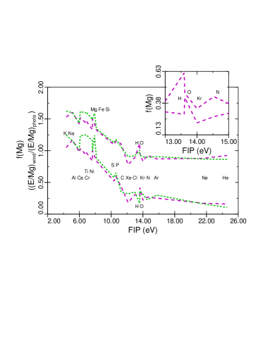
Figure 1.— Left: Schematic showing FIP fractionation in open and closed field regions. In both cases, waves impinge on footpoints from below, but the closed field can also have wave generation within the corona. Right: Model element fractionation in open (top, shifted up by 0.5 for clarity) and closed field (bottom). The result shown here is for model 1 (see Table 1). Green short dash lines show ponderomotive acceleration only; purple long dash lines show combined effect of ponderomotive acceleration and adiabatic invariant conservation. The inset shows the region around H, O, Kr, and N in more detail, for fast wind (top) and slow wind (bottom), for the combined model only. Note that the fractionation ratio O/H $>1$ in the slow wind, but is $<1$ in the fast wind.

The FIP fractionation, including the depletion of He, is most faithfully reproduced in a model of a closed coronal loop where the Alfvén waves are resonant (Laming, 2012, 2017; Rakowski & Laming, 2012), so that the coronal loop acts as a resonant cavity, where the Alfvén wave travel time from one footpoint to the other is an integral number of wave half periods. Although it is possible for waves ultimately deriving from convection within the solar envelope to enter coronal loops at footpoints and propagate into the corona, typically the periods of these waves (three or five minutes) are too long for resonance. Resonant waves are most plausibly excited within the coronal loop itself, most likely as a byproduct of the mechanism(s) that heat the corona (Dahlburg et al., 2016). In open field regions, such a resonance does not exist, and only waves propagating up from footpoints are possible. In such a scenario, the difference in fractionation between fast wind which originates in open magnetic field structures on the Sun, and slow wind which originates in closed coronal loops which are subsequently opened up by interchange reconnection (e.g. Lynch et al., 2014), arises naturally due to the extra resonant waves. Figure 1 (left panel) gives a schematic illustration of the open and closed field models, and the right panel illustrates the different fractionation patterns (see below for fuller discussion).

2. Model Calculations

The fractionation is calculated in each case by solving Alfvén wave transport equations in a model coronal structure. In the open field region a spectrum of Alfvén waves is chosen to match those given in Cranmer & van Ballegooijen (2005) and Cranmer et al. (2007) high up in the corona, and integrated back to the chromosphere. In the closed loop, we take a single Alfvén wave corresponding to the fundamental of a 75,000 km long loop having a 10 G coronal magnetic field, combined with two additional photospheric waves with periods of three and five minutes (e.g. Heggland et al., 2011). All waves are taken to be shear (planar) Alfvén waves (Laming, 2017). The instantaneous ponderomotive acceleration, $a$, is given by

$$a={c^{2}\over 2}{\partial\over\partial z}\left(\delta E^{2}\over B^{2}\right)$$ (1)

where $\delta E$ is the wave electric field, $B$ the ambient magnetic field, $c$ the speed of light, and $z$ is a coordinate along the magnetic field. The element fractionation, $f_{p}$, is calculated from ratios of densities $\rho_{k}$ for element $k$ at upper and lower boundaries of the fractionation region $z_{u}$ and $z_{l}$ respectively, as given by the equation (Laming, 2017)

$$f_{p} = {\rho_{k}\left(z_{u}\right)\over\rho_{k}\left(z_{l}\right)}$$ (2)

$$= \exp\left\{\int_{z_{l}}^{z_{u}}{2\xi_{k}a\nu_{kn}/\left[\xi_{k}\nu_{kn}+\left(1-\xi_{k}\right)\nu_{ki}\right]\over 2k_{\rm B}T/m_{k}+v_{||,osc}^{2}+2u_{k}^{2}}dz\right\},$$

where $\xi_{k}$ is the element ionization fraction, $\nu_{ki}$ and $\nu_{kn}$ are collision frequencies of ions and neutrals with the background gas (mainly hydrogen and protons), $k_{\rm B}T/m_{k}\left(=v_{z}^{2}\right)$ represents the square of the element thermal velocity along the $z$-direction, $u_{k}$ is the upward flow speed and $v_{||,osc}$ a longitudinal oscillatory speed, corresponding to upward and downward propagating sound waves. Because $\nu_{ki}>>\nu_{kn}$ in the fractionation region at the top of the chromosphere, small departures of $\xi_{k}$ from unity can result in large decreases in the fractionation.

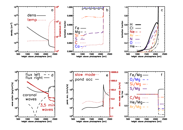
Figure 2.— The chromospheric model. (a) shows the density and temperature structure of the chromosphere. (b) shows chromospheric ionization fractions for low FIP elements and (c) for high FIP elements. (d) shows the wave energy fluxes in each direction for the three waves in the closed loop model. (e) shows the ponderomotive acceleration (solid line) and the amplitude of slow mode waves induced by the Alfvén wave driver. (f) shows the fractionations resulting for selected elements relative to Mg. Gas pressure and magnetic field pressure are equal at about 1000 km, magnetic field pressure dominating at higher altitudes.

Isotopic fractionation between fast and slow solar wind has also been observed in the Genesis data. Specifically, lighter isotopes are more abundant relative to heavy ones of the same element in the slow wind compared to the fast (Heber et al., 2012a). This is the opposite of what would be expected from equation 2, where with increased ponderomotive acceleration, $a$, a heavier isotope would have a smaller thermal speed and hence a higher value of $f_{p}$. An extra mass dependent fractionation (MDF) mechanism must be present. Inefficient Coulomb drag (ICD) has frequently been discussed, especially in connection with the depletion of He in the solar wind (Bodmer & Bochsler, 1998; Bochsler, 2007b). This depletion is now part of the FIP fractionation. During the Genesis data collection period, there is little other evidence for ICD in data collected by Genesis, Wind (Kasper et al., 2012), or the Advanced Composition Explorer (ACE; Pilleri et al., 2015) in element abundances (the solar minimum of 2007-8 might be a different matter). ICD should be strongest in the fast wind emanating along open field lines in coronal holes, with slow wind originating in closed loops more fully mixed by waves and turbulence; the opposite of what we see.

We argue therefore that the MDF of isotopes is most likely due to the conservation of the first adiabatic invariant, in conditions where the ion gyrofrequency $\Omega=eB/m_{k}c>>1/\tau_{coll}>>v_{ex}/R$. The first inequality means that an ion executes many gyro-orbits around the magnetic field line in the time between Coulomb collisions with other ions, $\tau_{coll}$, and thus the magnetic flux enclosed by its orbit is conserved. Hence $Br_{g}^{2}\propto\left(v_{x}^{2}+v_{y}^{2}\right)/B=v_{\perp}^{2}/B$ is constant ($r_{g}$ is the particle gyroradius), giving rise to an acceleration

$${dv_{z}\over dt}=-{1\over 2}{dB\over dz}{v_{\perp}^{2}\over B}$$ (3)

in conditions where $v^{2}=v_{z}^{2}+v_{\perp}^{2}$ is constant. The second inequality expresses the condition that the plasma remain otherwise collisional, in that Coulomb collision frequencies are much greater than the expansion rate (wind speed, $v_{ex}$, divided by radius, $R$) of the solar wind, and local abundance enhancements in the corona can be sustained by increased diffusion up from the solar photosphere. This is necessarily a loose concept, and so our approach is to calculate the FIP fractionation for open and closed field according to the models outlined above, and then the add in mass dependent fractionation (which arises because the thermal speeds $v_{\perp}^{2}$ and $2k_{\rm B}T/m_{k}$ are proportional to $1/m_{k}$, while $v_{||,osc}^{2}$ and $u_{k}^{2}$ representing fluid motions are not, and are usually much larger)

$$f_{a}=\exp\left\{-\int{{dB/dz}\left(v_{\perp}^{2}/B\right)\over 2k_{\rm B}T/m_{k}+v_{||,osc}^{2}+2u_{k}^{2}}dz\right\},$$ (4)

to match the isotopic differences between high speed and low speed solar wind. The region of integration in equation 4 is in the corona, out to a heliocentric distance of $1.5-2R_{\sun}$, where the corona is sufficiently collisionless to allow solar wind acceleration to commence (Cranmer et al., 1999; Miralles et al., 2001). Figure 1 (right panel) shows the resulting fractionations relative to Mg for open (top curves, shifted upwards by 0.5 for clarity) and closed field (bottom). The green lines indicate the effect of the ponderomotive acceleration only, the purple curves show the combined effect of ponderomotive acceleration and the adiabatic invariant conservation. Elements lighter (heavier) than Mg are enhanced (depleted) in abundance by the adiabatic invariant.

Figure 2 illustrates some important features of the FIP fractionation in closed loops, based on the chromospheric model of Avrett & Loeser (2008). Top left (a) shows the density and temperature structure of the chromosphere. Top middle (b) shows chromospheric ionization fractions for low FIP elements, and top right (c) for high FIP elements. Bottom left (d) shows the wave energy fluxes in each direction for the three wave frequencies considered, the wave resonant with the coronal loop, and three and five minute waves propagating up from the photosphere. Bottom middle (e) shows the ponderomotive acceleration (solid line) and the amplitude of slow mode waves induced by the Alfvén wave driver. Bottom right (f) shows the fractionations resulting for selected elements relative to Mg. The ponderomotive acceleration has a strong “spike” at an altitude of 2150 km, where the chromospheric density gradient is steep (see top left), resulting in strong fractionation at this height.

Table 1Isotopic Fractionations

Ratio	Model 1 (low MDF)	Model 2 (high MDF)	Observations
3He/4He	-4.6%	-5.3%	$6.31\pm 0.21$% 1
20Ne/22Ne	0.46% amu-1	0.41% amu-1	$0.42\pm 0.05$% amu-1 1
36Ar/38Ar	0.25% amu-1	0.20% amu-1	$0.26\pm 0.05$% amu-1 1
$f_{FIP,slow}$	2.69	2.73	2.652
$f_{FIP,fast}$	1.91	1.99	2.032
$B_{freeze,slow}/B_{\sun}$	0.1353	0.1053	0.0944
$B_{freeze,fast}/B_{\sun}$	0.3683	0.2353	0.1734

3. Results & Discussion

We compare the measured fractionations from Genesis samples with models designed to match the solar wind conditions during the Genesis period, and seek a “best fit”. In this paper, as a short cut, we construct individual fast and slow wind models (including the adiabatic invariant), given above in Figure 1 (right panel). These have been tuned to match the observed FIP fractionations given by Pilleri et al. (2015), defined as the sum of the FIP fractionations for Fe, Mg, and Si divided by the sum of those for C, O, and Ne. We assume a time fraction 0.35 during this time period due to fast wind, and 0.65 from slow wind and coronal mass ejections (CMEs), assumed to be similarly fractionated (Pilleri et al., 2015). This then matches the ratio of Mg fluences in fast and slow wind/CMEs, $\left(0.35f_{FIPfast}\right)/\left(0.65f_{FIPslow}\right)$ given by Heber et al. (2014).

Further details of these models are given in Table 1. The assumed diminution of magnetic field, which controls the adiabatic invariant acceleration, is compared to that estimated from Wang & Sheeley (1990). These authors give values for $B_{s}\left(R_{s}\right)$ at $R_{s}=2.5R_{\sun}$ relative to its value on the solar surface. We estimate the magnetic field decrease at $1.5-2.0R_{\sun}$ where the solar wind decouples collisonally from the sun to be approximately $\sqrt{B_{S}\left(R_{S}=2.5R_{\sun}\right)/B_{\sun}}$ and compare this with our assumed model values in Table 1. We assume representative speeds of 450 and 600 km s^-1 for slow and fast wind respectively (Pilleri et al., 2015). We emphasize that this magnetic field decrease represents the least constrained free parameter in the model, and is chosen to match existing solar observations, and in combination with the FIP fractionation reproduce data from both ACE and Genesis simultaneously.

We give two models with differing amounts of mass dependent fractionation (MDF) corresponding to different magnetic field expansions, $B_{freeze}/B_{\sun}$, yielding different isotopic fractionations. Both models have been specified to reproduce the observed fractionation between fast and slow wind in ²⁰Ne/²²Ne and ³⁶Ar/³⁸Ar, as given in Heber et al. (2012a). The ratio ³He/⁴He shows similar behaviour that is not accounted for, due to other by now well known processes involving the resonant absorption of ion-cyclotron waves that arises for ${}^{3}He$ alone because of its unusual charge to mass ratio of 2/3. These enhance the ³He abundance (e.g. Bučik et al., 2014) and are currently not included in our model. Table 1 shows that the adjusted model slow-fast wind difference in both Ne and Ar isotopic compositions match well with Genesis data.

In Table 2 we compare isotopic fractionations derived by application of models 1 and 2 to the Genesis results with previous inferences in the literature. The modeled fractionations of ¹⁴N/¹⁵N, ¹⁶O/¹⁸O and ²⁵Mg/²⁶Mg are given for the combined fast and slow, i.e. bulk solar wind observed by Genesis, and compared with observations where they exist. Agreement is quite good, with the Sun isotopically lighter than other solar system bodies (c.f. Ayres et al., 2013). By combining our N model fractionations with the Genesis solar wind ¹⁴N/¹⁵N of Marty et al. (2011) we calculate photospheric ¹⁴N/¹⁵N ratios (Table 2) which can be compared with values for Jupiter and Saturn, often presumed to have formed from the the same pre-solar nebula material accreting the same N₂ as the Sun.

Figure 3 shows the predicted elemental fractionation for bulk (i.e. time integrated) solar wind collected by Genesis. The left and right panels give results for models 1 and 2 as given in Table 1, which have lesser and greater degrees of mass dependent fractionation by conservation of the first adiabatic invariant respectively. The two models give very similar FIP plots. The symbols in Figure 3 (same in both panels) give the measured Genesis fractionations relative to the photospheric abundances of Asplund et al. (2009), Scott et al. (2015a, b) and Grevesse et al. (2015). The Genesis results are K, Na, Rieck et al. (2016); Ca, Al, Cr, Heber et al. (2014); Fe, Mg, Jurewicz et al. (2011); C, N, O, Heber et al. (2013); Kr, Xe, Meshik et al. (2014); and H, Koeman-Shields et al. (2016).

The overall agreement between theory and data on Figure 3 is quite good. Inclusion of the adiabatic invariant is a non-negotiable part of the model; it is required to provide the good matches in isotopic ratios shown in Table 1. Exclusion of the adiabatic invariant makes little difference for high FIP elements in Figure 3. The results excluding the adiabatic invariant better match the magnitude of the observed f(Mg) in Figure 3 for the low FIP range between Na and Mg; however the low FIP trend of the Genesis data is better matched by including the adiabatic invariant but the predicted magnitudes low FIP F(Mg) between Na and Mg are slightly too low relative to the data. Both models predict a small Fe/Mg fractionation that is not present in the data.

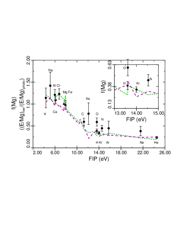
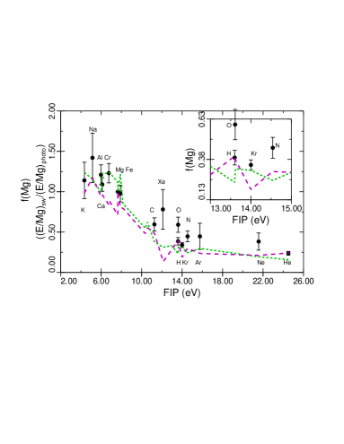
Figure 3.— Modeled fractionation patterns for Models 1 (left; low MDF) and 2 (right; high MDF) from Table 1. In each plot, the short dashed green line shows fractionation due to the ponderomotive acceleration alone, and long dashed purple curve shows the effect of ponderomotive acceleration and adiabatic invariant conservation. Symbols with error bars show results from Genesis data analysis. Model 2 assumes a higher mass dependent fractionation from the adiabatic invariant conservation. Model results for Kr and Xe assume the same ionization balance as for Ar.

Table 2Solar N and O Isotopic Abundances

Ratio	Model 1	Model 2	Observations
	(low MDF)	(high MDF)
16O/18O1	0.8 - 0.9	1.57 - 1.62	2.23	3.24
25Mg/26Mg1	0.5 - 0.8	1.14 - 1.40	$\simeq 1$ 5
14N/15N1	0.8 - 1.0	1.63 - 1.68	6
14N/15N2	4557	4527	400 - 714	$>500^{8}$

Our models are based on fractionations relative to Asplund et al. (2009) as observed with ACE by Pilleri et al. (2015). The most accurate Genesis data are for Ca, Mg, Fe, H, and He, and we have emphasized the match to these in tuning our models. There are no true photospheric abundances for Ar and Ne; Kr is accurate, but is based on an interpolated CI chondrite solar abundance. As noted, the adiabatic invariant model is only slightly below the low FIP (+C) data. The model agrees well with the high FIP H and He (plus Kr) data; it is distinctly below the O and N points.

The upward displacement of the O and N fractionations above the model curves in Fig. 3 may indicate that the photospheric abundances assumed for these elements are too small. The latest revision of CNO photospheric abundances (Asplund et al., 2009; Grevesse et al., 2015; Scott et al., 2015a, b) has recently been challenged by von Steiger & Zurbuchen (2016), who argue that fast solar wind from polar coronal holes is unfractionated and can be used to determine solar metallicity. A solar model based on this composition (Vagnozzi et al., 2017) has been criticized by Serenelli et al. (2016). Although fast wind from polar coronal holes can be considerably less fractionated than the fast wind seen in the ecliptic by Genesis, a complete absence of FIP effect is not always supported by coronal hole models of FIP fractionation, (Laming, 2012, 2015). However the application of our FIP models to the Genesis data analyzed to date supports the conclusion of von Steiger & Zurbuchen (2016), and is also more consistent with higher values obtained previously by Caffau et al. (2008), or even earlier by Grevesse & Sauval (1998).

The minimum amount by which the O abundance should increase to bring the error bar into contact with the model is 0.06-0.14 dex (for Models 1 and 2 respectively), which moves the abundance from 8.69 of Asplund et al. (2009) to 8.75 - 8.83, in better agreement with Caffau et al. (2008) and/or Grevesse & Sauval (1998). For comparison, Ayres et al. (2013) give an O abundance of 8.75, and more recently Cubas Armas et al. (2017) give $8.86\pm 0.04$, both based on spectroscopy.

The error bars on the Genesis data are one sigma, thus it is important to await further analyses, especially of low and high speed regime samples. The model result is driven by the fast wind model, for which the fractionation ratio O/H $<1$ (see Figure 1b), but this is fundamentally a polar coronal hole model applied to fast wind observed in the ecliptic. Measurements of the slow wind abundance ratio O/H would remove this uncertainty. The possibility exists once this is done of achieving a rather complete assessment of the elemental and isotopic composition of the solar photosphere as a proxy for the pre-solar nebula, by methods completely independent of those employed to date.

References

- Asplund et al. (2009) Asplund, M., Grevesse, N., Sauval, A. J., & Scott, P. 2009, Ann. Rev. Astron. Astrophys. 47, 481
- Avrett & Loeser (2008) Avrett, E. H., & Loeser, R. 2008, ApJS, 175, 229
- Ayres et al. (2013) Ayres, T. R., Lyons, J. R., Ludwig, H.-G., Caffau, E., & Wedemeyer-Böhm, S. 2013, ApJ, 765, 46
- Bochsler (2007a) Bochsler, P. 2007, A&A Rev, 14, 1
- Bochsler (2007b) Bochsler, P. 2007, A&A, 471, 315
- Bodmer & Bochsler (1998) Bodmer, R., & Bochsler, P. 1998, A&A, 337, 921
- Bučik et al. (2014) Bučik, R., Innes, D. E., Mall, U., Korth, A., Mason, G. M., & Gómez-Herrero, R. 2014, ApJ, 786, 71
- Burnett (2013) Burnett, D. S. 2013, Meteoritics & Planetary Science, 48, 2351
- Burnett et al. (2017) Burnett, D. S., Guan, Y., Heber, V. S. et al. 2017, LPI, 48, 1532
- Caffau et al. (2008) Caffau, E., Ludwig, H.-G., Steffen, M., Ayres, T. R., Bonifacio, P., Cayrel, R., Freytag, B., & Plez, B. 2008, A&A, 488, 1031
- Cranmer et al. (1999) Cranmer, S. R., Kohl, J. L., Noci, G., et al. 1999, ApJ, 511, 481
- Cranmer & van Ballegooijen (2005) Cranmer, S. R., & van Ballegooijen, A. A. 2005, ApJS, 156, 265
- Cranmer et al. (2007) Cranmer, S. R., van Ballegooijen, A. A., & Edgar, R. J. 2007, ApJS, 171, 520
- Cubas Armas et al. (2017) Cubas Armas, M., Asensio Ramos, A., & Socas-Navarro, H. 2017, A&A, 600, A45
- Dahlburg et al. (2016) Dahlburg, R. B., Laming, J. M., Taylor, B. D., & Obenschain, K. 2016, ApJ, 831, 160
- De Pontieu et al. (2007) De Pontieu, B., McIntosh, S., Carlsson, M. et al. 2007,2007, Science, 318, 1574
- Fletcher et al. (2014) Fletcher, L. N., Greathouse, T. K., Orton, G. S., Irwin, P. G., Mousis, O., Sinclair, J. A., & Giles, R. S. 2014, Icarus, 238, 170
- Grevesse & Sauval (1998) Grevesse, N., & Sauval, A. J. 1998, Space Sci. Rev. 85, 161
- Grevesse et al. (2015) Grevesse, N., Scott, P., Asplund, M., & Sauval, A. J. 2015, A&A, 573, A26
- Heber et al. (2009) Heber, V. S., Vogel, N., Wieler, R., & Burnett, D. S. 2009, Geochimica et Cosmochimica Acta Supp., 73, A509
- Heber et al. (2012a) Heber, V. S., Baur, H., Bochsler, P., McKeegan, K. D., Neugebauer, M., Reisenfeld, D. B., Wieler, R., & Wiens, R. C. 2012a, ApJ, 759, 121
- Heber et al. (2012b) Heber, V. S., Jurewicz, A. J. G., Janney, P., Wadhwa, M., McKeegan, K. D., & Burnett, D. S. 2012b, LPI, 43, 2921
- Heber et al. (2013) Heber, V. S., Burnett, D. S., Duprat, J., Guan, Y., Jurewicz, A. J. G., Marty, B., & McKeegan, K.D. 2013, LPI, 44, 2540
- Heber et al. (2014) Heber, V. S., McKeegan, K. D., Smith, S., Jurewicz, A. J. G., Olinger, C., Burnett, D. S., & Guan, Y. 2014, LPI, 45, 1203
- Heggland et al. (2011) Heggland, L., Hansteen, V. H., De Pontieu, B., & Carlsson, M. 2011,ApJ, 743, 142
- Jurewicz et al. (2011) Jurewicz, A. J. G., Burnett, D. S., Woolum, D. S., McKeegan, K. D., Heber, V. S., Guan, Y., Humayun, M., & Hervig, R. 2011, LPI, 42, 1917
- Kasper et al. (2012) Kasper, J. C., Stevens, M. L., Korreck, K. E., Maruca, B. A., Kiefer, K. K., Schwadron, N. A., & Lepri, S. T. 2012, ApJ, 745, 162
- Koeman-Shields et al. (2016) Koeman-Shields, E. C., Huss, G. R., Ogliore, R. C., Jurewicz, A. J. G., Burnett, D. S., Nagashiima, K., & Olinger, C. Y. 2016, LPI, 47, 2800
- Laming (2004) Laming, J. M. 2004, ApJ, 614, 1063
- Laming (2009) Laming, J. M. 2009, ApJ, 695, 954
- Laming (2012) Laming, J. M. 2012, ApJ, 744, 115
- Laming (2015) Laming, J. M. 2015, LRSP, 12, 2
- Laming (2017) Laming, J. M. 2017, ApJ, 844, 153
- Lynch et al. (2014) Lynch, B. J., Edmondson, J. K., & Li, Y. 2014, Solar Phys., 289, 3043
- Marty et al. (2011) Marty, B., Chaussidon, M., Wiens, R. C., Jurewicz, A. J. G., & Burnett, D. S. 2011, Science, 332, 1533
- McKeegan et al. (2011) McKeegan, K. D., Kallio, A. P. A., Heber, V. S., et al. 2011, Science, 332, 1528
- Meshik et al. (2014) Meshik, A., Hohenberg, C., Pravdivtseva, O., & Burnett, D. 2014, Geochim. Cosmochim, 127, 326
- Miralles et al. (2001) Miralles, M. P., Cranmer, S. R., & Kohl, J. L. 2001, ApJ, 560, L193
- Pilleri et al. (2015) Pilleri, P., Reisenfeld, D. B., Zurbuchen, T. H., Lepri. S. T., Shearer, P., Gilbert, J. A., von Steiger, R., & Wiens, R. C. 2015, ApJ, 812, 1
- Pottasch (1963) Pottasch, S. R. 1963, ApJ, 137, 945
- Rakowski & Laming (2012) Rakowski, C. E., & Laming, J. M., 2012, ApJ, 754, 65
- Rieck et al. (2016) Rieck, K., Jurewicz, A. J. G., Burnett, D. S., Hervig, R. L., Williams, P., & Guan, Y. 2016, LPI, 47, 2922
- Scott et al. (2015a) Scott, P., Asplund, M., Grevesse, N., Bergemann, M., & Sauval, A. J. 2015, A&A, 573, A26
- Scott et al. (2015b) Scott, P., Grevesse, N., Asplund, M., et al. 2015, A&A, 573, A25
- Serenelli et al. (2016) Serenelli, A., Scott, P., Villante, F. L., Vincent, A. C., Asplund, M., Basu, S., Grevesse, N., & Peña-Garay, C. 2016, MNRAS, 463, 2
- Vagnozzi et al. (2017) Vagnozzi, S., Freese, K., & Zurbuchen, TY. H. 2017, ApJ, 839, 55
- von Steiger & Zurbuchen (2016) von Steiger, R., & Zurbuchen, T. H. 2016, ApJ, 816, 13
- Wang & Sheeley (1990) Wang, Y.-M., & Sheeley, N. R. 1990, ApJ, 355, 726