Quasiparticle anisotropic hydrodynamics for ultrarelativistic heavy-ion collisions

Abstract:

In this proceedings contribution, we will review the basics of quasiparticle anisotropic hydrodynamics. Then, we will present some recent phenomenological results of 3+1d quasiparticle anisotropic hydrodynamics and Pb-Pb $2.76$ TeV collisions from the ALICE collaboration. We show that 3+1d quasiparticle anisotropic hydrodynamics model is able to describe the experimental results for Pb-Pb collisions at $2.76$ TeV quite well for many observables such as the spectra, the elliptic flow, and HBT radii in many centrality classes.

1 Introduction

The quark-gluon plasma (QGP) can be created and studied using heavy-ion collision experiments at the Relativistic Heavy Ion Collider (RHIC) and Large Hadron Collider (LHC). Their results show that in a broad energy range the collective behavior of the created QGP may be described within ideal or, even more precisely, with viscous relativistic hydrodynamics. [1, 2, 3, 4]. However, to properly account for the high-momentum anisotropies that exists in the QGP, anisotropic hydrodynamics was introduced [5, 6, 7, 8, 9, 10, 11]. In the recent few years, there have been many theoretical advancements in anisotropic hydrodynamics, but with limited phenomenological comparisons. Earlier this year, we were able to present some phenomenological comparisons using non-conformal anisotropic hydrodynamics. For recent reviews about anisotropic hydrodynamics, we refer the reader to [12, 13].

In this proceedings contribution, we will introduce anisotropic hydrodynamics and then focus on a specific approache, quasiparticle anisotropic hydrodynamics. In quasiparticle anisotropic hydrodynamics, one introduces a single finite-temperature dependent quasiparticle mass. This thermal mass can be determined using the realistic equation of state (EoS) which is provided by lattice measurements. Then, by some modification on the conformal EoS formalism of anisotropic hydrodynamics [10, 14] one can make a self-consistent non-conformal framework called quasiparticle anisotropic hydrodynamics (aHydroQP). As usual, the dynamical equations are obtained by taking moments of the Boltzmann equation with the appropriate bulk variables for the quasiparticles. After obtaining the dynamical equations, we present some phenomenological comparisons between aHydroQP and ALICE collaboration data for a few observables.

2 Anisotropic hydrodynamics

In anisotropic hydrodynamics, one assumes the one-particle distribution function to be of the form

$$f(x,p)=f_{\rm iso}\!\left(\frac{1}{\lambda}\sqrt{p_{\mu}\Xi^{\mu\nu}p_{\nu}}\right)+\delta f(x,p),$$ (1)

where $\lambda$ is the scale parameter which can be identified with the temperature in the isotropic equilibrium limit and $\xi^{\mu\nu}$ is the anisotropy tensor [10]

$$\Xi^{\mu\nu}=u^{\mu}u^{\nu}+\xi^{\mu\nu}-\Delta^{\mu\nu}\Phi\,,$$ (2)

where $u^{\mu}$ is the fluid four-velocity, $\xi^{\mu\nu}$ is a symmetric and traceless anisotropy tensor, and $\Phi$ is the degree of freedom associated with the bulk pressure since our system in this case is non-conformal. Within leading-order anisotropic hydrodynamics considered here one assumes $\delta f=0$, thus we ignore $\delta f$ contributions. We also assume $\xi^{\mu\nu}$ to be diagonal since the off-diagonal elements of $\xi^{\mu\nu}$ are small [12].

In the local rest frame the distribution function in Eq. (1) takes the following compact form

$$f(x,p)=f_{\rm eq}\!\left(\frac{1}{\lambda}\sqrt{\sum_{i}\frac{p_{i}^{2}}{\alpha_{i}^{2}}+m^{2}}\right),$$ (3)

where $i\in\{x,y,z\}$ and $\alpha_{i}\equiv(1+\xi_{i}+\Phi)^{-1/2}\,$. We note that by taking $\alpha_{x}=\alpha_{y}=\alpha_{z}=1$ and $\lambda=T$ one recovers the isotropic equilibrium distribution function which, in the classical case, is given by $f_{e\rm q}(T)=\exp(-E/T)$.

3 Quasiparticle anisotropic hydrodynamics (aHydroQP)

In this approach, in order to take into account the non-conformality of the QGP, we assume that the QGP can be described as an ensemble of massive quasiparticles with a single temperature-dependent mass $m(T)$. Since lattice QCD results [15] provide us with the equilibrium energy density and pressure one may use the following thermodynamic identity to find $m(T)$

$$\epsilon_{\rm eq}+P_{\rm eq}=TS_{\rm eq}=4\pi\tilde{N}T^{4}\,\hat{m}_{\rm eq}^{3}K_{3}\left(\hat{m}_{\rm eq}\right),$$ (4)

with $\hat{m}_{\rm eq}=m/T$. Since we will have extra terms generated by the gradients of the mass, we need to add a background field to the energy-momentum tensor to ensure thermodynamic consistency. In this case, the energy momentum tensor is defined by

$$T^{\mu\nu}_{\rm eq}=T^{\mu\nu}_{\rm kinetic,eq}+g^{\mu\nu}B_{\rm eq}\,,$$ (5)

where $B_{\rm eq}$ is the equilibrium background field which can be easily determined by integrating the following equation [16]

$$\frac{dB_{\rm eq}}{dT}=-4\pi\tilde{N}m^{2}TK_{1}(\hat{m}_{\rm eq})\frac{dm}{dT}\,,$$ (6)

We refer the reader to [16, 17, 18, 19, 20] for more details about aHydroQP framework.

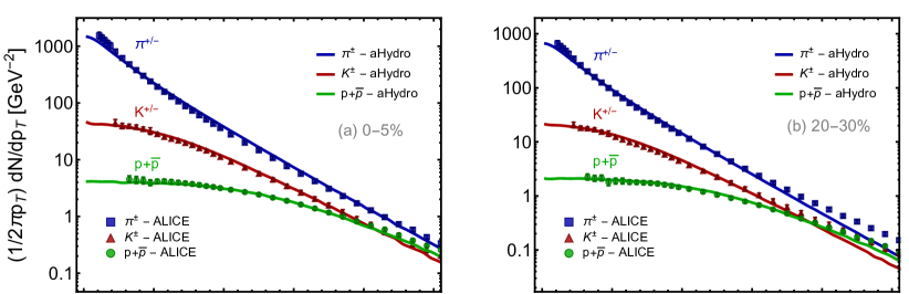
Figure 1: Transverse momentum spectra of $\pi^{\pm}$, $K^{\pm}$, and $p+\bar{p}$ in 0-5% and 20-30% centrality classes as shown in each panel. Solid lines are aHydroQP predictions and data are taken from [21].

4 3+1d quasiparticle anisotropic hydrodynamics

Next, we turn to our quasiparticle anisotropic hydrodynamics dynamical equations for 3+1d relativistic massive quasiparticle systems. To obtain the dynamical equations, one takes moments of the Boltzmann equation for particles with masses which depend on the local environment, e.g. the temperature [16]

$$p^{\mu}\partial_{\mu}f(x,p)+\frac{1}{2}\partial_{i}m^{2}\partial^{i}_{(p)}f(x,p)=-C[f(x,p)]\,,$$ (7)

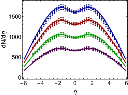
Figure 2: In the left panel, $\langle p_{T}\rangle$ of pions, kaons, and protons is shown as a function of centrality. In the right panel, the charged-hadron multiplicity as a function of pseudorapidity is shown in 0-5%, 5-10%, 10-20%, and 20-30% centrality classes. Data are from the ALICE collaboration Ref. [21] and Refs. [22, 23] for left panel and right panel respectively.

where $f(x,p)$ is the anisotropic distribution function specified in Eq. (3) and $C[f(x,p)]$ is the collisional kernel. As we can see in the Boltzmann equation, the second term on the left-hand side corresponds to the gradients of the mass since it is a function of temperature and $T$ is a function of space-time. In practice, it suffices to take the lower-order moments, i.e., zeroth, first, and second moments to obtain the dynamical equations

$$\partial_{\mu}J^{\mu} = -\int\!dP\,\,C[f]\,,$$ (8)

$$\partial_{\mu}T^{\mu\nu} = -\int\!dP\,p^{\nu}\,C[f]\,,$$ (9)

$$\partial_{\mu}I^{\mu\nu\lambda}-J^{(\nu}\partial^{\lambda)}m^{2} = -\int\!dP\,p^{\nu}p^{\lambda}\,C[f]\,,$$ (10)

where $J^{\mu}$, $T^{\mu\nu}$, and $I^{\mu\nu\lambda}$ are the particle four-current, the energy-momentum tensor, and the rank-three tensor, respectively, defined by

$$J^{\mu} \equiv \int\!dP\,p^{\mu}f(x,p)\,,$$ (11)

$$T^{\mu\nu} \equiv \int\!dP\,p^{\mu}p^{\nu}f(x,p)+B({\bm{\alpha}},\lambda)g^{\mu\nu},$$ (12)

$$I^{\mu\nu\lambda} \equiv \int\!dP\,p^{\mu}p^{\nu}p^{\lambda}f(x,p)\,.$$ (13)

with $B({\bm{\alpha}},\lambda)$ being the non-equilibrium background field which can be found requiring thermodynamic consistency similar to the equilibrium case by this differential equation

$$\partial_{\mu}B=-\frac{1}{2}\partial_{\mu}m^{2}\int\!dPf(x,p)\,.$$ (14)

Below we will list the dynamical equations in 3+1d aHydroQP. Taking the projections of the energy momentum tensor $u_{\nu}\partial_{\mu}T^{\mu\nu}$, $X_{\nu}\partial_{\mu}T^{\mu\nu}$, $Y_{\nu}\partial_{\mu}T^{\mu\nu}$, and $Z_{\nu}\partial_{\mu}T^{\mu\nu}$ one gets the following four equations

$$D_{u}\epsilon+\epsilon\theta_{u}+P_{x}u_{\mu}D_{x}X^{\mu}+P_{y}u_{\mu}D_{y}Y^{\mu}+P_{z}u_{\mu}D_{z}Z^{\mu} = 0\,,$$ (15)

$$D_{x}P_{x}+P_{x}\theta_{x}-\epsilon X_{\mu}D_{u}u^{\mu}-P_{y}X_{\mu}D_{y}Y^{\mu}-P_{z}X_{\mu}D_{z}Z^{\mu} = 0\,,$$ (16)

$$D_{y}P_{y}+P_{y}\theta_{y}-\epsilon Y_{\mu}D_{u}u^{\mu}-P_{x}Y_{\mu}D_{x}X^{\mu}-P_{z}Y_{\mu}D_{z}Z^{\mu} = 0\,,$$ (17)

$$D_{z}P_{z}+P_{z}\theta_{z}-\epsilon Z_{\mu}D_{u}u^{\mu}-P_{x}Z_{\mu}D_{x}X^{\mu}-P_{y}Z_{\mu}D_{y}Y^{\mu} = 0\,.$$ (18)

Figure 3: The identified elliptic flow coefficient as a function of $p_{T}$ is shown for $\pi^{\pm}$, $K^{\pm}$, and $p+\bar{p}$ in 20-30% and 30-40% centrality classes. The experimental data shown are from the ALICE collaboration  [24].

where $D_{u}=u_{\mu}\partial^{\mu}$, $D_{x}=X_{\mu}\partial^{\mu}$, $D_{y}=Y_{\mu}\partial^{\mu}$, $D_{z}=Z_{\mu}\partial^{\mu}$, $\theta_{u}=\partial_{\mu}u^{\mu}$, $\theta_{x}=\partial_{\mu}X^{\mu}$, $\theta_{y}=\partial_{\mu}Y^{\mu}$, and $\theta_{z}=\partial_{\mu}Z^{\mu}$. Another three equations are obtained from the diagonal projections of the second moment, i,e., $X_{\nu}X_{\lambda}\partial_{\mu}I^{\mu\nu\lambda}$, $Y_{\nu}Y_{\lambda}\partial_{\mu}I^{\mu\nu\lambda}$, and $Z_{\nu}Z_{\lambda}\partial_{\mu}I^{\mu\nu\lambda}$

$$D_{u}I_{x}+I_{x}(\theta_{u}+2u_{\mu}D_{x}X^{\mu}) = \frac{1}{\tau_{\rm eq}}(I_{\rm eq}-I_{x})\,,$$ (19)

$$D_{u}I_{y}+I_{y}(\theta_{u}+2u_{\mu}D_{y}Y^{\mu}) = \frac{1}{\tau_{\rm eq}}(I_{\rm eq}-I_{y})\,,$$ (20)

$$D_{u}I_{z}+I_{z}(\theta_{u}+2u_{\mu}D_{z}Z^{\mu}) = \frac{1}{\tau_{\rm eq}}(I_{\rm eq}-I_{z})\,.$$ (21)

Finally, one can use the matching condition to get the last equation which relates the scale parameter $\lambda$ and the effective temperature $T$

$$\epsilon_{\rm kinetic}(\lambda)=\epsilon_{\rm kinetic,eq}(T)\,.$$ (22)

For the definitions of $I_{u}$, $I_{i}$, $I_{\rm eq}$, one can refer to Ref. [16].

5 Phenomenological results

We now turn to the phenomenological results. We show comparisons between 3+1d quasiparticle anisotropic hydrodynamics and the experimental data from ALICE collaboration for 2.76 TeV Pb+Pb collisions. For more comparisons, see Refs. [19, 20]. In this model we assumed that $\eta/s={\rm const}$, we used smooth Glauber initial conditions, and we used isotropic initial conditions $\alpha_{i}(\tau=0)=1$. To perform the hadronic freeze-out we used a customized version of THERMINATOR 2 [25].

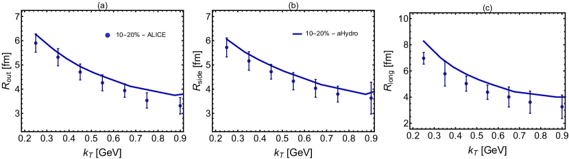
Figure 4: The femtoscopic Hanbury-Brown-Twiss (HBT) radii as a function of the pair mean transverse momentum for $\pi^{+}\pi^{+}$ is shown for 10-20% centrality class. In the top row, the left, middle, right panels show $R_{\rm out}$, $R_{\rm side}$, and $R_{\rm long}$ respectively. In the bottom row, the left, middle, right panels show $R_{\rm out}/R_{\rm side}$, $R_{\rm out}/R_{\rm long}$, and $R_{\rm side}/R_{\rm long}$ respectively. All results are for 2.76 TeV Pb+Pb collisions where data shown are for $\pi^{\pm}\,\pi^{\pm}$ combined from the ALICE collaboration [26].

Let us start by showing the spectra of pions, kaons, and protons as a function of the transverse momentum $p_{T}$ in Fig. 1. In this figure, we show the spectra in 0-5% and 20-30% centrality classes. As can be seen from Fig. 1, our model provides a good description of the spectra and shows the mass splitting between different hadron species. Next, in Fig. 2-a, the average transverse momentum as a function of centrality is shown where aHydroQP agrees with the data quite well. In Fig. 2-b, we show the multiplicity as a function of pseudorapidity in four centrality classes as shown in the figure. As we can see from this figure, aHydroQP describes the multiplicity very well compared with experimental data.

We next show the identified elliptic flow as a function of $p_{T}$ in two different centrality classes 20-30% and 30-40% in Fig. 3. As can be seen from this figure, our model shows a good agreement with experimental results up to $p_{T}\sim 1.5$ GeV. Finally, in the top row and bottom row of Fig. 4, we show comparisons of HBT radii $R_{\rm out}$, $R_{\rm side}$, and $R_{\rm long}$ and HBT radii ratios $R_{\rm out}/R_{\rm side}$, $R_{\rm out}/R_{\rm long}$, and $R_{\rm side}/R_{\rm long}$, respectively, as a function of the average transverse momentum. For results of other centrality classes see Ref. [20]. As can be seen from this figure, aHydroQP predictions are in a good agreement with the experimental data.

Finally, we would like to list the extracted fitting parameters that we used in these comparisons which are $T_{0}(\tau_{0}=0.25$ fm/c$)=600$ MeV, $\eta/s=0.159$, and $T_{\rm FO}=130$ MeV. In Fig. 5, we show the bulk viscosity predicted by our model aHydroQP compared with other two models: Bayesian analysis and black hole engineering where they all have good agreement “magnitude wise”. We note here that we used $\eta/s=0.159$ in this plot.

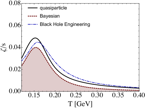
Figure 5: We show the temperature dependence of the bulk viscosity scaled by the entropy density ($\zeta/S$) obtained using quasiparticle anisotropic hydrodynamics (solid-black line). For sake of comparison, we show some other model predictions: Bayesian analysis [27], and black hole engineering [28].

6 Conclusions and outlook

In this proceedings contribution, we showed how one can derive the dynamical equations of 3+1d quasiparticle anisotropic hydrodynamics. And how one can enforce thermodynamic consistency using the quasiparticle description in kinetic theory approaches (anisotropic hydrodynamics was an example here). We next showed some experimental comparisons with ALICE collaboration data and listed our fitting parameters extracted from fits to ALICE experimental data. Then we showed some observables like the spectra, the mean transverse momentum as a function of centrality, the elliptic flow as a function of the mean transverse momentum, and HBT radii. In most observables, our model (aHydroQP) was able to describe the data quite well with only a few fit parameters.

Looking to the future, we are working on a few improvements to our model. For example, we are working on including temperature-dependent shear viscosity to entropy density ratio, i.e., $\eta/s(T)$. We are also planning to compare with RHIC highest energies in the near future. Moreover, we are setting up the pipeline for using fluctuating initial conditions in our code.

References

- [1] P. Huovinen, P. F. Kolb, U. W. Heinz, P. V. Ruuskanen and S. A. Voloshin, Radial and elliptic flow at RHIC: further predictions, Phys. Lett. B503 (2001) 58–64, [hep-ph/0101136].
- [2] P. Romatschke and U. Romatschke, Viscosity Information from Relativistic Nuclear Collisions: How Perfect is the Fluid Observed at RHIC?, Phys. Rev. Lett. 99 (2007) 172301, [0706.1522].
- [3] S. Ryu, J. F. Paquet, C. Shen, G. S. Denicol, B. Schenke, S. Jeon et al., Importance of the Bulk Viscosity of QCD in Ultrarelativistic Heavy-Ion Collisions, Phys. Rev. Lett. 115 (2015) 132301, [1502.01675].
- [4] H. Niemi, G. S. Denicol, P. Huovinen, E. Molnár and D. H. Rischke, Influence of the shear viscosity of the quark-gluon plasma on elliptic flow in ultrarelativistic heavy-ion collisions, Phys.Rev.Lett. 106 (2011) 212302, [1101.2442].
- [5] W. Florkowski and R. Ryblewski, Highly-anisotropic and strongly-dissipative hydrodynamics for early stages of relativistic heavy-ion collisions, Phys.Rev. C83 (2011) 034907, [1007.0130].
- [6] M. Martinez and M. Strickland, Dissipative Dynamics of Highly Anisotropic Systems, Nucl. Phys. A848 (2010) 183–197, [1007.0889].
- [7] M. Martinez, R. Ryblewski and M. Strickland, Boost-Invariant (2+1)-dimensional Anisotropic Hydrodynamics, Phys.Rev. C85 (2012) 064913, [1204.1473].
- [8] R. Ryblewski and W. Florkowski, Highly-anisotropic hydrodynamics in 3+1 space-time dimensions, Phys. Rev. C85 (2012) 064901, [1204.2624].
- [9] D. Bazow, U. W. Heinz and M. Strickland, Second-order (2+1)-dimensional anisotropic hydrodynamics, Phys.Rev. C90 (2014) 054910, [1311.6720].
- [10] M. Nopoush, R. Ryblewski and M. Strickland, Bulk viscous evolution within anisotropic hydrodynamics, Phys.Rev. C90 (2014) 014908, [1405.1355].
- [11] M. Nopoush, R. Ryblewski and M. Strickland, Anisotropic hydrodynamics for conformal Gubser flow, Phys. Rev. D91 (2015) 045007, [1410.6790].
- [12] M. Strickland, Anisotropic Hydrodynamics: Three lectures, Acta Phys. Polon. B45 (2014) 2355–2394, [1410.5786].
- [13] M. Alqahtani, M. Nopoush and M. Strickland, “Relativistic anisotropic hydrodynamics - A review.” forthcoming, 2017.
- [14] M. Nopoush, M. Strickland, R. Ryblewski, D. Bazow, U. Heinz and M. Martinez, Leading-order anisotropic hydrodynamics for central collisions, Phys. Rev. C92 (2015) 044912, [1506.05278].
- [15] S. Borsanyi, G. Endrodi, Z. Fodor, A. Jakovac, S. D. Katz et al., The QCD equation of state with dynamical quarks, JHEP 1011 (2010) 077, [1007.2580].
- [16] M. Alqahtani, M. Nopoush and M. Strickland, Quasiparticle equation of state for anisotropic hydrodynamics, Phys. Rev. C92 (2015) 054910, [1509.02913].
- [17] M. Alqahtani, M. Nopoush and M. Strickland, Quasiparticle anisotropic hydrodynamics for central collisions, Phys. Rev. C95 (2017) 034906, [1605.02101].
- [18] M. Alqahtani and M. Strickland, Quasiparticle anisotropic hydrodynamics, in Hot Quarks 2016: Workshop for Young Scientists on the Physics of Ultrarelativistic Nucleus-Nucleus Collisions (HQ2016) South Padre Island, Texas, September 12-17, 2016, 2016, 1610.07643, http://inspirehep.net/record/1494418/files/arXiv:1610.07643.pdf.
- [19] M. Alqahtani, M. Nopoush, R. Ryblewski and M. Strickland, 3+1d quasiparticle anisotropic hydrodynamics for ultrarelativistic heavy-ion collisions, Phys. Rev. Lett. 119 (2017) 042301, [1703.05808].
- [20] M. Alqahtani, M. Nopoush, R. Ryblewski and M. Strickland, Anisotropic hydrodynamic modeling of 2.76 TeV Pb-Pb collisions, Phys. Rev. C96 (2017) 044910, [1705.10191].
- [21] ALICE collaboration, B. Abelev et al., Centrality dependence of , K, p production in Pb-Pb collisions at = 2.76 TeV, Phys. Rev. C88 (2013) 044910, [1303.0737].
- [22] ALICE collaboration, E. Abbas et al., Centrality dependence of the pseudorapidity density distribution for charged particles in Pb-Pb collisions at = 2.76 TeV, Phys. Lett. B726 (2013) 610–622, [1304.0347].
- [23] ALICE collaboration, J. Adam et al., Centrality evolution of the charged-particle pseudorapidity density over a broad pseudorapidity range in Pb-Pb collisions at 2.76 TeV, Phys. Lett. B754 (2016) 373–385, [1509.07299].
- [24] ALICE collaboration, B. B. Abelev et al., Elliptic flow of identified hadrons in Pb-Pb collisions at TeV, JHEP 06 (2015) 190, [1405.4632].
- [25] M. Chojnacki, A. Kisiel, W. Florkowski and W. Broniowski, THERMINATOR 2: THERMal heavy IoN generATOR 2, Comput. Phys. Commun. 183 (2012) 746–773, [1102.0273].
- [26] ALICE collaboration, A. K. Graczykowski, Pion femtoscopy measurements in ALICE at the LHC, EPJ Web Conf. 71 (2014) 00051, [1402.2138].
- [27] S. A. Bass, J. E. Bernhard and J. S. Moreland, Determination of Quark-Gluon-Plasma Parameters from a Global Bayesian Analysis, in 26th International Conference on Ultrarelativistic Nucleus-Nucleus Collisions (Quark Matter 2017) Chicago,Illinois, USA, February 6-11, 2017, 2017, 1704.07671, http://inspirehep.net/record/1594915/files/arXiv:1704.07671.pdf.
- [28] R. Rougemont, R. Critelli, J. Noronha-Hostler, J. Noronha and C. Ratti, Dynamical versus equilibrium properties of the QCD phase transition: A holographic perspective, Phys. Rev. D96 (2017) 014032, [1704.05558].