Estimates for the best constant in a Markov $L_{2}$–inequality with the assistance of computer algebra

Abstract

We prove two-sided estimates for the best (i.e., the smallest possible) constant $\,c_{n}(\alpha)\,$ in the Markov inequality

$$\|p_{n}^{\prime}\|_{w_{\alpha}}\leq c_{n}(\alpha)\|p_{n}\|_{w_{\alpha}}\,,\qquad p_{n}\in{\cal P}_{n}\,.$$

Here, ${\cal P}_{n}$ stands for the set of algebraic polynomials of degree $\leq n$, $\,w_{\alpha}(x):=x^{\alpha}\,e^{-x}$, $\,\alpha>-1$, is the Laguerre weight function, and $\|\cdot\|_{w_{\alpha}}$ is the associated $L_{2}$-norm,

$$\|f\|_{w_{\alpha}}=\left(\int_{0}^{\infty}|f(x)|^{2}w_{\alpha}(x)\,dx\right)^{1/2}\,.$$

Our approach is based on the fact that $\,c_{n}^{-2}(\alpha)\,$ equals the smallest zero of a polynomial $\,Q_{n}$, orthogonal with respect to a measure supported on the positive axis and defined by an explicit three-term recurrence relation. We employ computer algebra to evaluate the seven lowest degree coefficients of $\,Q_{n}\,$ and to obtain thereby bounds for $\,c_{n}(\alpha)$. This work is a continuation of a recent paper [5], where estimates for $\,c_{n}(\alpha)\,$ were proven on the basis of the four lowest degree coefficients of $\,Q_{n}$.

Keywords: Markov type inequalities, orthogonal polynomials, Laguerre weight function, three-term recurrence relation, computer algebra.

2000 Math. Subject Classification: 41A17

1 Introduction and statement of the results

Throughout this paper $\,{\cal P}_{n}\,$ will stand for the set of algebraic polynomials of degree at most $~{}n$, assumed, without loss of generality, with real coefficients. Let $\,w_{\alpha}(x):=x^{\alpha}\,e^{-x}$, where $\alpha>-1$, be the Laguerre weight function, and $\,\|\cdot\|_{w_{\alpha}}\,$ be the associated $L_{2}$-norm,

$$\|f\|_{w_{\alpha}}=\left(\int_{0}^{\infty}|f(x)|^{2}w_{\alpha}(x)\,dx\right)^{1/2}\,.$$

We study the best constant $\,c_{n}(\alpha)\,$ in the Markov inequality in this norm

$$\|p_{n}^{\prime}\|_{w_{\alpha}}\leq c_{n}(\alpha)\|p_{n}\|_{w_{\alpha}}\,,\qquad p_{n}\in{\cal P}_{n}\,,$$ (1.1)

namely the constant

$$c_{n}(\alpha):=\sup_{p_{n}\in{\cal P}_{n}}\frac{\|p_{n}^{\prime}\|_{w_{\alpha}}}{\|p_{n}\|_{w_{\alpha}}}\,.$$

Before formulating our results, let us give a brief account on the results known so far.

It is only the case $\,\alpha=0\,$ where the best Markov constant is known, namely, Turán [9] proved that

$$c_{n}(0)=\Big{(}2\sin\frac{\pi}{4n+2}\Big{)}^{-1}\,.$$

Dörfler [2] showed that $c_{n}(\alpha)={\cal O}(n)$ for every fixed $\,\alpha>-1\,$ by proving the estimates

$$c_{n}^{2}(\alpha)\geq\frac{n^{2}}{(\alpha+1)(\alpha+3)}+\frac{(2\alpha^{2}+5\alpha+6)\,n}{3(\alpha+1)(\alpha+2)(\alpha+3)}+\frac{\alpha+6}{3(\alpha+2)(\alpha+3)}\,,\vspace*{2mm}$$ (1.2)

$$c_{n}^{2}(\alpha)\leq\frac{n(n+1)}{2(\alpha+1)}\,,$$ (1.3)

see [3] for a more accessible source. In the same paper, [3], Dörfler proved for the asymptotic constant

$$c(\alpha):=\lim_{n\rightarrow\infty}\frac{c_{n}(\alpha)}{n}\,,$$ (1.4)

that

$$c(\alpha)=\frac{1}{j_{(\alpha-1)/2,1}}\,,$$ (1.5)

where $j_{\nu,1}$ is the first positive zero of the Bessel function $J_{\nu}(z)$ .

Nikolov and Shadrin obtained in [5] the following result:

Theorem A ([5, Theorem 1]). For all $\,\alpha>-1\,$ and $\,n\in\mathbb{N}\,$, $\,n\geq 3\,$, the best constant $\,c_{n}(\alpha)\,$ in the Markov inequality (1.1) admits the estimates

$$\frac{2\big{(}n+\frac{2\alpha}{3}\big{)}\big{(}n-\frac{\alpha+1}{6}\big{)}}{(\alpha+1)(\alpha+5)}<c_{n}^{2}(\alpha)<\frac{\big{(}n+1\big{)}\big{(}n+\frac{2(\alpha+1)}{5}\big{)}}{(\alpha+1)\big{[}(\alpha+3)(\alpha+5)\big{]}^{1/3}}\,,$$ (1.6)

where for the left-hand inequality it is additionally assumed that $\,n>(\alpha+1)/6$ .

Theorem A implies some inequalities for the asymptotic Markov constant $\,c(\alpha)\,$ and, through (1.5), inequalities for $\,j_{\nu,1}\,$, the first positive zero of the Bessel function $\,J_{\nu}\,$ (see [5, Corollaries 1, 3]). It was also shown in [5, Theorem 2] that $\,c(\alpha)={\cal O}(\alpha^{-1})\,$, which indicates that the upper estimate for $\,c_{n}(\alpha)\,$ in Theorem A, though rather good for moderate $\,\alpha\,$, is not optimal.

In a recent paper [7] Nikolov and Shadrin proved an upper bound for $\,c_{n}(\alpha)\,$ which is of the correct order with respect to both $\,n\,$ and $\,\alpha\,$ as they tend to infinity.

Theorem B ([7, Theorem 1.1]). For all $\,n\in\mathbb{N}\,$, $\,n\geq 3\,$, the best constant $\,c_{n}(\alpha)\,$ in the Markov inequality (1.1) satisfies the inequality

$$c_{n}^{2}(\alpha)\leq\frac{4n\big{(}n+2+\frac{3(\alpha+1)}{4}\big{)}}{\alpha^{2}+10\alpha+8}\,,\qquad\alpha\geq 2\,.$$ (1.7)

As a consequence of Theorem B and Dörfler’s lower bound (1.2) for $\,c_{n}(\alpha)\,$ Nikolov and Shadrin showed that

$$c_{n}^{2}(\alpha)\asymp\frac{n(n+\alpha+3)}{(\alpha+1)(\alpha+8)}\,,\qquad n\geq 3,\ \alpha\geq 2\,.$$

Corollary C ([7, Corollary 1.1]). For all $\,\alpha\geq 2\,$ and $\,n\geq 3\,$ the best constant $\,c_{n}(\alpha)\,$ in the Markov inequality (1.1) satisfies

$$\frac{2n(n+\alpha+3)}{3(\alpha+1)(\alpha+8)}\leq c_{n}^{2}(\alpha)\leq\frac{4n(n+\alpha+3)}{(\alpha+1)(\alpha+8)}\,.$$ (1.8)

In addition, Nikolov and Shadrin found the limit value of $\,(\alpha+1)c_{n}^{2}(\alpha)\,$ as $\,\alpha\to-1$, and proved asymptotic inequalities for $\,\alpha\,c_{n}^{2}(\alpha)\,$ as $\,\alpha\rightarrow\infty\,$.

Corollary D ([7, Corollary 1.2]). The best constant $\,c_{n}(\alpha)\,$ in the Markov inequality (1.1) satisfies:

(i)   $\displaystyle\lim_{\alpha\rightarrow-1}(\alpha+1)c_{n}^{2}(\alpha)=\frac{n(n+1)}{2}\,$;

(ii)   $\displaystyle\frac{2n}{3}\leq\lim_{\alpha\to\infty}\alpha\,c_{n}^{2}(\alpha)\leq 3n\,$.

A combination of Theorem A and Theorem B implies some inequalities for the asymptotic Markov constant (1.4):

Corollary E ([7, Corollary 1.2]). The asymptotic Markov constant $\,c(\alpha)=\lim\limits_{n\to\infty}\dfrac{c_{n}(\alpha)}{n}\,$ satisfies the inequalities

$$\frac{2}{(\alpha+1)(\alpha+5)}<c^{2}(\alpha)<\begin{cases}\,\dfrac{1}{(\alpha+1)\sqrt[3]{(\alpha+3)(\alpha+5)}}\,,&\quad-1<\alpha\leq\alpha^{*}\,,\vspace*{1mm}\\ \,\dfrac{4}{\alpha^{2}+10\alpha+8}\,,&\quad\alpha>\alpha^{*}\,,\end{cases}$$

where $\alpha^{*}\approx 43.4$ .

The ratio of the upper and the lower bound for $\,c(\alpha)\,$ in Corollary E is less than $\,\sqrt{2}\,$ for all $\,\alpha>-1\,$.

In this paper we investigate the best Markov constant $\,c_{n}(\alpha)\,$ following the approach from [5]. It is known (see Proposition 2.1 below) that $\,c_{n}^{-2}(\alpha)\,$ is equal to the smallest zero of a polynomial $\,Q_{n}\,$, which is orthogonal with respect to a measure supported on $\,\mathbb{R}_{+}\,$. Since $\,\{Q_{n}\}_{n\in\mathbb{N}}\,$ are defined by an explicit three-term recurrence relation, one can evaluate (at least theoretically) as many coefficients of $\,Q_{n}\,$ as necessary. With the assistance of Wolfram’s Mathematica we find the seven lowest degree coefficients of the polynomial $\,Q_{n}\,$, and thereby the six highest degree coefficients of $\,R_{n}\,$, the monic polynomial reciprocal to $\,Q_{n}\,$. Then we apply a simple technique for estimating the largest zero $\,x_{n}\,$ of $\,R_{n}\,$ on the basis of its $k$ highest degree coefficients, $\,3\leq k\leq 6\,$, thus obtaining lower and upper bounds for $\,c_{n}^{2}(\alpha)\,$. Our main result in this paper is:

Theorem 1.1.

For $\,3\leq k\leq 6\,$ and for all $\,n\geq k\,$, the best constant $\,c_{n}(\alpha)\,$ in the Markov inequality (1.1) admits the estimates

$$\underline{c}_{\,n,k}(\alpha)\leq c_{n}(\alpha)\leq\overline{c}_{n,k}(\alpha)\,,\qquad\alpha>-1\,,$$ (1.9)

where

$$\underline{c}_{\,n,3}^{2}(\alpha)=\frac{2\,n\big{(}n+\frac{3(\alpha+1)}{8}\big{)}}{(\alpha+1)(\alpha+5)}\,,$$ (1.10)

$$\overline{c}_{n,3}^{\>2}(\alpha)=\frac{(n+1)\big{(}n+\frac{2(\alpha+1)}{5}\big{)}}{(\alpha+1)\big{[}(\alpha+3)(\alpha+5)\big{]}^{1/3}}\,,$$ (1.11)

$$\underline{c}_{\,n,4}^{2}(\alpha)=\frac{(5\alpha+17)\,n\big{(}n+\frac{8(\alpha+1)}{25}\big{)}}{2(\alpha+1)(\alpha+3)(\alpha+7)}\,,$$ (1.12)

$$\overline{c}_{n,4}^{\>2}(\alpha)=\frac{(5\alpha+17)^{1/4}(n+1)\big{(}n+\frac{3(\alpha+1)}{7}\big{)}}{(\alpha+1)(\alpha+3)^{1/2}\big{[}2(\alpha+5)(\alpha+7)\big{]}^{1/4}}\,,$$ (1.13)

$$\underline{c}_{\,n,5}^{2}(\alpha)=\frac{2(7\alpha+31)n\big{(}n+\frac{25(\alpha+1)}{84}\big{)}}{(\alpha+1)(\alpha+9)(5\alpha+17)}\,,$$ (1.14)

$$\overline{c}_{n,5}^{\>2}(\alpha)=\frac{(7\alpha+31)^{1/5}(n+1)\big{(}n+\frac{4(\alpha+1)}{9}\big{)}}{(\alpha+1)(\alpha+3)^{2/5}\big{[}(\alpha+5)(\alpha+7)(\alpha+9)\big{]}^{1/5}}\,,$$ (1.15)

$$\underline{c}_{\,n,6}^{2}(\alpha)=\frac{\big{(}21\alpha^{3}+299\alpha^{2}+1391\alpha+2073\big{)}n\big{(}n+\frac{2(\alpha+1)}{7}\big{)}}{(\alpha+1)(\alpha+3)(\alpha+5)(\alpha+11)(7\alpha+31)}\,,$$ (1.16)

$$\overline{c}_{n,6}^{\>2}(\alpha)=\frac{\big{(}21\alpha^{3}+299\alpha^{2}+1391\alpha+2073\big{)}^{1/6}(n+1)\big{(}n+\frac{5(\alpha+1)}{11}\big{)}}{(\alpha+1)(\alpha+3)^{1/2}(\alpha+5)^{1/3}\big{[}(\alpha+7)(\alpha+9)(\alpha+11)\big{]}^{1/6}}\,.$$ (1.17)

Remark 1.2.

For $\,3\leq k\leq 6$, the pair $\,\big{(}\underline{c}_{\,n,k}(\alpha),\overline{c}_{\,n,k}(\alpha)\big{)}\,$ of bounds for $\,c_{n}(\alpha)\,$ is deduced with the use of the $\,k\,$ highest degree coefficients of the polynomial $\,R_{n}\,$ (and (1.11) is the upper bound obtained in [5]). Generally, the bounds for $\,c_{n}(\alpha)\,$ obtained with larger $\,k\,$ are better, although some exceptions are observed for small $\,n\,$ and $\,\alpha\,$.

Clearly, inequalities (1.9) imply bounds for the asymptotic Markov constant $\,c(\alpha)\,$. Here, it is not difficult to prove that the larger $\,k\,$, the better the implied lower and upper bounds for $\,c(\alpha)\,$, hence the best bounds for $\,c(\alpha)\,$ are obtained from (1.9) with $\,k=6\,$.

Thus, Theorem 1.1 yields an improvement of the estimates for the asymptotic Markov constant $\,c(\alpha)\,$ in Corollary E.

Corollary 1.3.

The asymptotic Markov constant $\,c(\alpha)=\lim\limits_{n\to\infty}n^{-1}c_{n}(\alpha)\,$ satisfies the inequalities

$$\underline{c}(\alpha)<c(\alpha)<\overline{c}(\alpha)\,,$$

where

$$\underline{c}^{2}(\alpha):=\frac{21\alpha^{3}+299\alpha^{2}+1391\alpha+2073}{(\alpha+1)(\alpha+3)(\alpha+5)(\alpha+11)(7\alpha+31)}$$

and

$$\overline{c}^{\>2}(\alpha):=\begin{cases}\dfrac{\big{(}21\alpha^{3}+299\alpha^{2}+1391\alpha+2073\big{)}^{1\!/6}}{(\alpha+1)(\alpha+3)^{1\!/2}(\alpha+5)^{1\!/3}\big{[}(\alpha+7)(\alpha+9)(\alpha+11)\big{]}^{1\!/6}}\,,&\!\!-1\!<\!\alpha\leq\alpha^{\star}\,,\vspace*{1mm}\\ \dfrac{4}{\alpha^{2}+10\alpha+8}\,,&\!\!\alpha>\alpha^{\star},\end{cases}$$

with $\,\alpha^{\star}\approx 172\,$.

It is worth noticing that the ratio of the upper and the lower bound for $\,c(\alpha)\,$ in Corollary 1.3 does no exceed $\,\frac{2\sqrt{3}}{3}\approx 1.1547\,$ for all $\,\alpha>-1\,$.

Theorem 1.1, in particular inequality (1.16), implies an improvement of the lower bound in Corollary D(ii).

Corollary 1.4.

The best constant $\,c_{n}(\alpha)\,$ in the Markov inequality (1.1) satisfies:

$$\frac{6n}{7}\leq\lim_{\alpha\to\infty}\alpha\,c_{n}^{2}(\alpha)\leq 3n\,.$$

The rest of the paper is organized as follows. Sect. 2 contains some preliminaries. In Sect. 2.1 we characterize the squared best Markov constant as the largest zero of an $n$-th degree monic polynomial $\,R_{n}\,$ with positive roots, and propose a recursive procedure for the evaluation of its coefficients (Proposition 2.2). Two-sided estimates for the largest zero of polynomials with only positive roots in terms of few of their coefficients are proposed in Sect. 2.2 (Proposition 2.3). The assisted by Wolfram’s Mathematica proof of our results is given in Sect. 3. In Sect. 4 we give some final remarks and conclusions, and formulate two conjectures concerning the asymptotic behaviour of the best Markov constant and the coefficients of the characteristic polynomial $\,R_{n}\,$.

2 Preliminaries

2.1 An orthogonal polynomial related to $c_{n}(\alpha)$

It is well-known that the squared best constant in a Markov-type inequality in $L_{2}$-norm is equal to the largest eigenvalue of a related positive definite $\,n\times n\,$ matrix $\,{\mathbf{A}}_{n}\,$, thus the problem of finding the best Markov constant is equivalent to evaluating the largest eigenvalue of $\,{\mathbf{A}}_{n}$. Perhaps, a less known fact is that for a wide class of $L_{2}$-norms, the inverse matrix $\,{\mathbf{A}}_{n}^{-1}\,$ is tri-diagonal, see [1, Sect. 2]. In the particular case of the $L_{2}$-norm induced by the Laguerre weight function $\,w_{\alpha}\,$ this connection is given by the following proposition:

Proposition 2.1 ([3, p. 85]).

The quantity $\,c_{n}^{-2}(\alpha)\,$ is equal to the smallest zero of the polynomial $\,Q_{n}(x)=Q_{n}(x,\alpha)\,$, which is defined recursively by

$$Q_{n+1}(x)=(x-d_{n})Q_{n}(x)-\lambda_{n}^{2}Q_{n-1}(x),\quad n\geq 0\,;$$

$$Q_{-1}(x):=0,\ \ Q_{0}(x):=1\,;$$

$$d_{0}:=1+\alpha,\ \ d_{n}:=2+\frac{\alpha}{n+1}\,,\quad n\geq 1\,;$$

$$\lambda_{0}>0\ \ \text{{\rm arbitrary}},\ \lambda_{n}^{2}:=1+\frac{\alpha}{n}\,,\quad n\geq 1\,.$$

By Favard’s theorem, for any $\,\alpha>-1\,$, $\,\{Q_{n}(x,\alpha)\}_{n=0}^{\infty}\,$ form a system of monic orthogonal polynomials. Since $\,Q_{n}\,$ is the characteristic polynomial of the inverse of a positive definite matrix (which is also positive definite), it follows that all the zeros of $\,Q_{n}\,$ are positive (and distinct). Consequently, $\,\{Q_{n}\}_{n=0}^{\infty}\,$ are orthogonal with respect to a measure supported on $\mathbb{R}_{+}$.

By Proposition 2.1, we have

$$Q_{n+1}(x)=\Big{(}x-2-\frac{\alpha}{n+1}\Big{)}Q_{n}(x)-\Big{(}1+\frac{\alpha}{n}\Big{)}Q_{n-1}(x)\,,\quad n\geq 1\,,$$ (2.1)

$$Q_{0}(x)=1\,,\quad Q_{1}(x)=x-\alpha-1\,.$$ (2.2)

If we write $\,Q_{n}\,$ in the form

$$Q_{n}(x)=x^{n}-a_{n-1,n}\,x^{n-1}+a_{n-2,n}\,x^{n-2}-\cdots+(-1)^{n}\,a_{0,n}\,,$$

then

$$a_{0,n}=\binom{n+\alpha}{n}\,,\qquad n\in\mathbb{N}_{0}\,,$$ (2.3)

with the convention that the right-hand side is equal to $1$ for $\,n=0\,$. The proof is by induction with respect to $n$. For $\,n=0,\,1\,$, (2.3) follows from (2.2). Assuming (2.3) is true for all $\,m\leq n\,$, we verify it for $\,m=n+1\,$ by putting $\,x=0\,$ in (2.1) and using the induction hypothesis:

$$(-1)^{n+1}a_{0,n+1} =\Big{(}2+\frac{\alpha}{n+1}\Big{)}(-1)^{n+1}\binom{n+\alpha}{n}+\Big{(}1+\frac{\alpha}{n}\Big{)}(-1)^{n}\binom{n-1+\alpha}{n-1}$$

$$=(-1)^{n+1}\binom{n+1+\alpha}{n}\,.$$

Now, instead of $\,\{Q_{n}\}_{n=0}^{\infty}\,$, we consider the sequence of orthogonal polynomials $\,\{\widetilde{Q}_{n}\}_{n=0}^{\infty}\,$ normalised so that $\,\widetilde{Q}_{n}(0)=1$ , $\,n\in\mathbb{N}_{0}\,$, i.e.,

$$Q_{n}(x)=(-1)^{n}\binom{n+\alpha}{n}\widetilde{Q}_{n}(x)\,,\qquad n\in\mathbb{N}_{0}\,.$$

It follows from (2.1) and (2.2) that $\,\{\widetilde{Q}_{n}\}_{n\in\mathbb{N}_{0}}\,$ are determined by

$$\Big{(}1+\frac{\alpha}{n+1}\Big{)}\widetilde{Q}_{n+1}(x)=\Big{(}2+\frac{\alpha}{n+1}-x\Big{)}\widetilde{Q}_{n}(x)-\widetilde{Q}_{n-1}(x)\,,\quad n\geq 1\,,$$ (2.4)

$$\widetilde{Q}_{0}(x)=1\,,\quad\widetilde{Q}_{1}(x)=1-\frac{x}{\alpha+1}\,.$$ (2.5)

Writing $\,\widetilde{Q}_{n}\,$ in the form

$$\widetilde{Q}_{n}(x)=1-A_{1,n}\,x+A_{2,n}\,x^{2}-\cdots+(-1)^{n}A_{n,n}\,x^{n}$$

and rewriting (2.4) as

$$\widetilde{Q}_{n+1}(x)-\widetilde{Q}_{n}(x)=\frac{n+1}{n+\alpha+1}\big{(}\widetilde{Q}_{n}(x)-\widetilde{Q}_{n-1}(x)\big{)}+\frac{n+1}{n+\alpha+1}\,x\,\widetilde{Q}_{n}(x)\,,\quad n\in\mathbb{N}\,,$$

we deduce the following recurrence relation for the evaluation of the coefficients $\,\{A_{i,m}\}\,$:

$$A_{i,n+1}-A_{i,n}=\frac{n+1}{n+\alpha+1}\big{(}A_{i,n}-A_{i,n-1}\big{)}+\frac{n+1}{n+\alpha+1}\,A_{i-1,n}\,,\ \ n\geq k\geq 1\,,$$ (2.6)

$$\text{with }A_{0,n}=1\ \text{ and }\ A_{1,1}=\frac{1}{\alpha+1}\,.$$

Since, by Proposition 2.1, $\,c_{n}^{-2}(\alpha)\,$ is equal to the smallest zero of $\,\widetilde{Q}_{n}\,$, it follows that $\,c_{n}^{2}(\alpha)\,$ equals the largest zero of the reciprocal polynomial of $\,\widetilde{Q}_{n}\,$,

$$R_{n}(x)=x^{n}\,\widetilde{Q}_{n}(1/x)\,.$$ (2.7)

The above observations allow us to reformulate Proposition 2.1 in the following equivalent form:

Proposition 2.2.

The squared best Markov constant $\,c_{n}^{2}(\alpha)\,$ is equal to the largest zero of the polynomial

$$R_{n}(x)=x^{n}-A_{1,n}\,x^{n-1}+A_{2,n}\,x^{n-2}-\cdots+(-1)^{n}A_{n,n}\,.$$ (2.8)

The coefficients of $\,R_{n}\,$ are evaluated recursively by the following procedure:

• $\,A_{1,1}=\frac{1}{\alpha+1}$ ;

• Set $\,A_{0,m}=1\,$, $\,m=0,\ldots,n\,$;

• For $i=1$ to $n$:

  1. Find the sequence $\,\{D_{i,m}\}_{m=i-1}^{n}\,$ as solution of the recurrence equation

     $$D_{i,m+1}=\frac{m+1}{m+\alpha+1}\,D_{i,m}+\frac{m+1}{m+\alpha+1}\,A_{i-1,m}$$ (2.9)

     with the initial condition $\,D_{i,i-1}=0\,$;

  2. Evaluate

     $$A_{i,n}=\sum_{m=i}^{n}D_{i,m}\,.$$ (2.10)

2.2 Polynomials with positive roots: bounds for the largest zero

Let $\,P\,$ be a monic polynomial of degree $\,n\,$ with zeros $\,\{x_{i}\}_{i=1}^{n}\,$,

$$P(x)=\prod_{i=1}^{n}(x-x_{i})=x^{n}-b_{1}\,x^{n-1}+b_{2}\,x^{n-2}-\cdots+(-1)^{n}b_{n}\,.$$

The coefficients $\,b_{r}=b_{r}(P)\,$, $\,r=1,\ldots,n\,$, are given by the elementary symmetric functions of $\,\{x_{i}\}_{i=1}^{n}\,$,

$$b_{r}=s_{r}=s_{r}(P)=\sum_{1\leq i_{1}<i_{2}<\cdots<i_{r}\leq n}x_{i_{1}}x_{i_{2}}\cdots x_{i_{r}}\,,\qquad r=1,\ldots,n\,.$$

It is well known that the elementary symmetric functions $\,\{s_{r}\}\,$ and the Newton functions (sums of powers of $\,x_{i}\,$)

$$p_{r}=p_{r}(P)=\sum_{i=1}^{n}x_{i}^{r}\,,\qquad r=1,2,3,\ldots\,,$$

are connected by the Newton identities:

$$p_{r}+\sum_{i=1}^{r-1}(-1)^{i}p_{r-i}\,s_{i}+(-1)^{r}r\,s_{r}=0\,,\qquad \text{if }\ 1\leq r\leq n\,,$$ (2.11)

$$p_{r}+\sum_{i=1}^{n}(-1)^{i}p_{r-i}\,s_{i}=0\,,\qquad \text{if }\ r>n\,.$$ (2.12)

For a proof, see e.g. [10] or [4].

Our interest in the Newton functions is motivated by the fact that they provide tight bounds for the largest zero of a polynomial whose roots are all positive. For any such polynomial $\,P\,$, we set

$$\ell_{k}(P):=\frac{p_{k}(P)}{p_{k-1}(P)}\,,\qquad u_{k}(P):=\big{[}p_{k}(P)\big{]}^{1/k}\,,\qquad k\in\mathbb{N}\,,$$

with the convention that $\,p_{0}(P):=\deg(P)\,$.

Proposition 2.3.

Let $\,P(x)=x^{n}-b_{1}\,x^{n-1}+b_{2}\,x^{n-2}-\cdots+(-1)^{n-1}b_{n-1}\,x+(-1)^{n}b_{n}\,$ be a polynomial with positive zeros $\,x_{1}\leq x_{2}\leq\cdots\leq x_{n}\,$.

Then the largest zero $\,x_{n}\,$ of $\,P\,$ satisfies the inequalities

$$\ell_{k}(P)\leq x_{n}<u_{k}(P)\,,\qquad k\in\mathbb{N}\,.$$ (2.13)

Moreover, the sequence $\,\{\ell_{k}(P)\}_{k=1}^{\infty}\,$ is monotonically increasing, the sequence $\,\{u_{k}(P)\}_{k=1}^{\infty}\,$ is monotonically decreasing, and

$$\lim_{k\to\infty}\ell_{k}(P)=\lim_{k\to\infty}u_{k}(P)=x_{n}\,.$$ (2.14)

Proof. For $\,i=1,\ldots,n-1\,$, we set $\,a_{i}:=\frac{x_{i}}{x_{n}}\,$, then $\,0<a_{i}\leq 1\,$. Now both inequalities (2.13) and the limit relations (2.14) readily follow from the representations

$$\ell_{k}(P)=\frac{a_{1}^{k}+\cdots+a_{n-1}^{k}+1}{a_{1}^{k-1}+\cdots+a_{n-1}^{k-1}+1}\,x_{n}\,,\qquad u_{k}(P)=\big{(}a_{1}^{k}+\cdots+a_{n-1}^{k}+1\big{)}^{1/k}x_{n}\,.$$

The monotonicity of the sequence $\,\{\ell_{k}(P)\}_{k=1}^{\infty}\,$ follows easily from Cauchy-Bouniakowsky’s inequality. Indeed, we have

$$\Big{(}\sum_{i=1}^{n}x_{i}^{k}\Big{)}^{2}=\Big{(}\sum_{i=1}^{n}x_{i}^{\frac{k-1}{2}}x_{i}^{\frac{k+1}{2}}\Big{)}^{2}\leq\Big{(}\sum_{i=1}^{n}x_{i}^{k-1}\Big{)}\Big{(}\sum_{i=1}^{n}x_{i}^{k+1}\Big{)}\,,$$

whence $\,p_{k}^{2}(P)\leq p_{k-1}(P)\,p_{k+1}(P)\,$, and consequently

$$\ell_{k}(P)=\frac{p_{k}(P)}{p_{k-1}(P)}\leq\frac{p_{k+1}(P)}{p_{k}(P)}=\ell_{k+1}(P)\,.$$

To prove monotonicity of the sequence $\,\{u_{k}(P)\}_{k=1}^{\infty}\,$, we recall that $\,0<a_{i}\leq 1\,$ and therefore $\,a_{i}^{k+1}\leq a_{i}^{k}\,$. We have

$$\big{(}a_{1}^{k+1}+\cdots+a_{n-1}^{k+1}+1\big{)}^{1/(k+1)}\!<\big{(}a_{1}^{k+1}+\cdots+a_{n-1}^{k+1}+1\big{)}^{1/k}\!\leq\big{(}a_{1}^{k}+\cdots+a_{n-1}^{k}+1\big{)}^{1/k},$$

which yields

$$u_{k+1}(P)<u_{k}(P)\,.$$

$\Box$

3 Computer algebra assisted proof of the results

Here we give the algorithms, the source code and the results of the computer algebra assisted proof of estimates (1.10)-(1.17) in Theorem 1.1. While the case $\,k=3\,$ and to a certain extent $\,k=4\,$ could be studied by hand, it seems impossible to provide similar calculations for larger $\,k\,$. We implement the idea from [5] for estimating $\,c_{n}(\alpha)\,$ using $\,k=3\,$ highest degree coefficients of the polynomial $\,R_{n}(x)\,$ and with the assistance of Wolfram’s Mathematica v. 10 software we investigate the cases $\,k=4,5,6\,$, as well. Software based on the algorithms described below failed with calculations for $\,k>6\,$.

For simplicity sake, henceforth we write the polynomial $\,R_{n}\,$ from (2.7) and (2.8) in the form

$$R_{n}(x)=x^{n}-b_{1}x^{n-1}+b_{2}x^{n-2}+\cdots+(-1)^{n}b_{n}\,.$$

3.1 Lower bounds for $c_{n}(\alpha)$

We apply Proposition 2.3 to estimate the largest zero $\,x_{n}=c_{n}^{2}(\alpha)\,$ of the polynomial $\,R_{n}(x)\,$ from below,

$$x_{n}\geq\ell_{k}(R_{n})=\frac{p_{k}(R_{n})}{p_{k-1}(R_{n})}\,,\qquad k=3,\,4,\,5,\,6\,,$$

and then with the help of computer algebra obtain a further estimation of the form

$$\ell_{k}(R_{n})\geq c\,n(n+\sigma(\alpha+1)),$$

with the optimal (i.e., the largest possible) constants $\,c=c(k)\,$ and $\,\sigma=\sigma(k)$.

Algorithm 1  Estimating $\,c_{n}(\alpha)\,$ from below

Input:	$\,k\in\{3,4,5,6\}\,$ – the number of the highest degree coefficients of $\,R_{n}(x)\,$
Step 1.	Express the power sums $\,p_{k-1}(R_{n})\,$ and $\,p_{k}(R_{n})\,$ in terms of $\,\{b_{i}\}_{i=1}^{k}\,$
Step 2.	Find coefficients $\,\{b_{i}\}_{i=1}^{k}\,$ in terms of $\,n\,$ and $\,\alpha\,$ using Proposition 2.2
Step 3.	Find a proper value $\,\sigma\,$ for parameter $\,s\,$ in $\,p_{k}-c\,n(n+s(\alpha+1))p_{k-1}\,$,
	where $\,c\,$ is the coefficient of $\,n^{2}\,$ in the quotient $\,p_{k}/p_{k-1}\,$
Step 4.	Represent the numerator of $\,f=p_{k}-c\,n(n+\sigma(\alpha+1))p_{k-1}\,$ in powers
	of $\,n\,$ and $\,(\alpha+1)\,$
Step 5.	Estimate from below the expression $\,f\,$ to prove that $\,f\geq 0\,$

Step 1:  Let $\,\{x_{i}\}_{i=1}^{n}\,$ be all the zeros of the polynomial $\,R_{n}(x)\,$ from (2.7). In order to express a power sum $\,p_{r}=\sum_{i=1}^{r}x_{i}^{r}\,$, $\,1\leq r\leq n$, by $\{b_{i}\}_{i=1}^{r}\,$, we apply the direct formula

$$p_{r}=\begin{vmatrix}b_{1}&1&0&\cdots&0\\ 2b_{2}&b_{1}&1&\cdots&0\\ 3b_{3}&b_{2}&b_{1}&\cdots&0\\ {5}\\ rb_{r}&b_{r-1}&b_{r-2}&\cdots&b_{1}\end{vmatrix}$$

which easily follows from the Newton identities (2.11).

Below is the code of the programme and the results for $\,k=1,\ldots,6\,$:

Step 2:  We find coefficients $\,\{b_{i}\}_{i=1}^{k}\,$ of the polynomial $\,R_{n}(x)\,$ using Proposition 2.2. For a fixed $\,i\,$ we firstly find a sequence solving recurrence equation (2.9) and then evaluate $\,b_{i}\,$ by (2.10).

The source and the results for $\,k=1,\ldots,6\,$ follow below:

Step 3:  The quotient $\,p_{k}/p_{k-1}\,$ is a quadratic polynomial in $\,n\,$, and we denote by $\,c\,$ its leading coefficient.

The goal of this step is to find a proper value (say $\sigma$) for parameter $\,s\,$ in the expression

$$f_{s}=p_{k}-c\,n(n+s(\alpha+1))p_{k-1}\,,$$

such that $\,f_{\sigma}\geq 0\,$ for all admissible $\,\alpha\,$ and $\,n\,$. For a fixed $\,k\,$ quantity $\,f_{s}\,$ depends on $\,\alpha\,$, $\,n\,$ and $\,s\,$. It is a polynomial of degree $\,2k-1\,$ in $\,n\,$ and a rational function in $\,\alpha\,$. Let us write the numerator of $\,f_{s}\,$ in the form

$$\sum_{i=1}^{2k-1}\sum_{j=0}^{d}\mu_{i,j}(s)(\alpha+1)^{d-j}n^{2k-i}\,.$$

The highest order coefficients in $\,\sum_{j}\mu_{i,j}(s)(\alpha+1)^{d-j}\,$ are linear functions in $\,s\,$ of the form $\,A_{i}-B_{i}s\,$, with $\,A_{i}>0\,$ and $\,B_{i}>0\,$. We denote their zeros by $\,s_{i}\,$ for each $\,i\,$ and set $\,\sigma=\min_{i}s_{i}\,$. Since we seek estimates valid for all $\,\alpha>-1\,$, our choice of $\,\sigma\,$ guarantee that for $\,\alpha\,$ sufficiently large the inequality $\,\sum_{j}\mu_{i,j}(s)(\alpha+1)^{d-j}>0\,$ holds true.

The code is as follows:

Table 1 gives results for the optimal values of $\,c\,$ and  $\sigma\,$ for $\,k=3,4,5,6\,$.

Table 1: The optimal values of $\,c\,$ and $\,\sigma\,$ in the lower bounds for $c_{n}^{2}(\alpha)$.

$k$	$c$	$\sigma$
3	$\dfrac{2}{(\alpha+1)(\alpha+5)}$	$\dfrac{3}{8}$
4	$\dfrac{5\alpha+17}{2(\alpha+1)(\alpha+3)(\alpha+7)}$	$\dfrac{8}{25}$
5	$\dfrac{2(7\alpha+31)}{(\alpha+1)(\alpha+9)(5\alpha+17)}$	$\dfrac{25}{84}$
6	$\dfrac{21\alpha^{3}+299\alpha^{2}+1391\alpha+2073}{(\alpha+1)(\alpha+3)(\alpha+5)(\alpha+11)(7\alpha+31)}$	$\dfrac{2}{7}$

Step 4: We set

$$f=p_{k}-c\,n(n+\sigma(\alpha+1))p_{k-1}=:\frac{\varphi(n,\alpha)}{\psi(\alpha)}$$

with $\,c\,$ and $\,\sigma\,$ determined in Step 3. Here, $\,\varphi(n,\alpha)\,$ is a bivariate polynomial in $\,n\,$ and $\,\alpha\,$, and $\,\psi(\alpha)\,$ is a polynomial in $\,\alpha\,$. More precisely, $\,\varphi(n,\alpha)\,$ has degree $\,2k-1\,$ in $\,n\,$, and degree $\,d\,$ in $\,\alpha\,$ which our programme calculates for each fixed $\,k\,$.

Note that $\,\psi(\alpha)>0\,$ for $\,\alpha>-1\,$ since it is a product of powers of $\,\alpha+j\,$, $\,j\geq 1\,$ and multipliers $\,A\alpha+B\,$, $\,0<A<B\,$. Therefore, $\,{\rm sign}\,f={\rm sign}\,\varphi\,$.

We expand $\,\varphi(n,\alpha)\,$ in the form

$$\varphi(n,\alpha)=\sum_{i=1}^{2k-1}\sum_{j=0}^{d}\mu_{i,j}(\alpha+1)^{d-j}n^{2k-i}=\begin{pmatrix}n^{2k-1}\\ n^{2k-2}\\ \vdots\\ n\end{pmatrix}^{\top}\mathbf{M}\begin{pmatrix}(\alpha+1)^{d}\\ (\alpha+1)^{d-1}\\ \vdots\\ 1\end{pmatrix}\,,$$

where $\,\mathbf{M}=\big{(}\mu_{i,j}\big{)}_{i=1,j=0}^{2k-1,d}\,$ and all entries $\,\mu_{i,j}\,$ are integer numbers.

The source for computation of the matrix $\,\mathbf{M}\,$ is listed below.

If $\,\mu_{i,j}\geq 0\,$ for all $\,i,j\,$, then $\,\varphi(n,\alpha)\geq 0\,$ and $\,f\geq 0\,$ for all $\,\alpha>-1\,$ and $\,n\geq k\,$. In a case some of coefficients $\,\mu_{i,j}<0\,$ we apply the next step of the algorithm.

The results for $\,k=3,4,5,6\,$ are given together with the estimates from Step 5.

Step 5:  If there are coefficients $\,\mu_{i,j}<0\,$ we need additional arguments to verify that $\,f\geq 0\,$ for all $\,\alpha>-1\,$ and $\,n\geq k\,$. We bring into use a new $\,(2k-1)\times(d+1)\,$ matrix $\,\mathbf{\Lambda}\,$ which elements we put initially $\,\lambda_{i,j}:=\mu_{i,j}\,$, for $\,i=1,\ldots,2k-1\,$ and $\,j=0,\ldots,d\,$.

The procedure described below checks recursively all coefficients $\,\lambda_{i,j}\,$ and makes the corresponding estimations. We need not introduce a new matrix after each iteration, but only replace a pair of elements in a column of $\,\mathbf{\Lambda}\,$ with new entries in such a manner that the value of the function

$$\Phi(\mathbf{\Lambda})=\sum_{i=1}^{2k-1}\sum_{j=0}^{d}\lambda_{i,j}(\alpha+1)^{d-j}n^{2k-i}=\begin{pmatrix}n^{2k-1}\\ n^{2k-2}\\ \vdots\\ n\end{pmatrix}^{\top}\mathbf{\Lambda}\begin{pmatrix}(\alpha+1)^{d}\\ (\alpha+1)^{d-1}\\ \vdots\\ 1\end{pmatrix}$$

decreases. At the end of the procedure we get a matrix $\,\mathbf{\Lambda}\,$ satisfying $\,\mathbf{0}\leq\mathbf{\Lambda}\leq\mathbf{M}\,$ (in the sense that $\,0\leq\lambda_{i,j}\leq\mu_{i,j}\,$ for all $\,i,j\,$) and therefore

$$0\leq\Phi(\mathbf{\Lambda})\leq\Phi(\mathbf{M})=\varphi(n,\alpha)\,.$$

Suppose that $\,\lambda_{i,j}<0\,$ for some pair of indices $\,i,j\,$. Then we set

$$h:=\min\{i-\eta:\lambda_{\eta,j}>0,\ 1\leq\eta\leq i-1\}\quad\text{and}\quad\delta:=\frac{\lambda_{i,j}}{k^{i-h}}\quad(\delta<0)\,.$$

If $\,\lambda_{h,j}+\delta\geq 0\,$, for $\,n\geq k\,$ we have

$$(\lambda_{h,j}+\delta)n^{2k-h}+0\,n^{2k-i} =\Big{(}\lambda_{h,j}+\frac{\lambda_{i,j}}{k^{i-h}}\Big{)}n^{2k-h}=\lambda_{h,j}n^{2k-h}+\lambda_{i,j}\frac{n^{2k-h}}{k^{i-h}}$$

$$\leq\lambda_{h,j}n^{2k-h}+\lambda_{i,j}\frac{n^{2k-h}}{n^{i-h}}=\lambda_{h,j}n^{2k-h}+\lambda_{i,j}{n^{2k-i}}\,.$$

Otherwise, if $\,\lambda_{h,j}+\delta<0\,$, for $\,n\geq k\,$ we have

$$0\,n^{2k-h}+\big{(}\lambda_{h,j}k^{i-h}+\lambda_{i,j}\big{)}n^{2k-i} =\lambda_{h,j}n^{2k-i}k^{i-h}+\lambda_{i,j}n^{2k-i}$$

$$\leq\lambda_{h,j}n^{2k-i}n^{i-h}+\lambda_{i,j}n^{2k-i}$$

$$\leq\lambda_{h,j}n^{2k-h}+\lambda_{i,j}n^{2k-i}\,.$$

So, replacing only two elements in $\,\mathbf{\Lambda}\,$,

$$\begin{cases}\lambda_{h,j}:=\lambda_{h,j}+\lfloor\delta\rfloor\ \ \qquad\,\text{and}\ \ \lambda_{i,j}:=0\,,&\text{ if }\lambda_{h,j}+\delta\geq 0,\\ \lambda_{i,j}:=\lambda_{h,j}\,k^{i-h}+\lambda_{i,j}\ \ \text{and}\ \ \lambda_{h,j}:=0\,,&\text{ otherwise },\end{cases}$$

we obtain that

$$\lambda_{h,j}(\alpha+1)^{d+1-j}n^{2k-h}+\lambda_{i,j}(\alpha+1)^{d+1-j}n^{2k-i}$$

decreases for the new values of $\,\lambda_{h,j}\,$ and $\,\lambda_{i,j}\,$, and hence $\,\Phi(\mathbf{\Lambda})\,$ also decreases.

Applying recursively the above iteration process for $\,i=2k-1,2k-2,\ldots,1\,$ and $\,j=0,1,\ldots,d\,$ we finally obtain a matrix $\,\mathbf{\Lambda}\,$ satisfying $\,\mathbf{0}\leq\mathbf{\Lambda}\leq\mathbf{M}\,$. Then $\,\varphi(n,\alpha)\geq 0\,$, $\,f\geq 0\,$ and therefore

$$c_{n}^{2}(\alpha)\geq\frac{p_{k}}{p_{k-1}}\geq c\,n(n+\sigma(\alpha+1))$$

for the optimal $\,c\,$ and $\,\sigma\,$ evaluated in Step 3. For $\,k=3,4,5,6\,$ we obtain estimates (1.10), (1.12), (1.14), and (1.16), respectively.

The following source implements the procedure described in Step 5.

Next, we give matrices $\,\mathbf{M}\,$ from Step 4 and $\,\mathbf{\Lambda}\,$ from Step 5 obtained with Mathematica.

Case $\,k=3\,$:

This partial case needs a special attention as we have to assume strict inequality $\,n>k\,$, i.e., $\,n\geq 4\,$, to obtain estimate (1.10). This causes a minor modification in Step 5 of Algorithm 1, namely, replacement of $\,k^{i-h}\,$ with $\,(k+1)^{i-h}\,$. Namely, we determine $\,\delta:=\lambda_{i,j}/(k+1)^{i-h}\,$ and set

$$\begin{cases}\lambda_{h,j}:=\lambda_{h,j}+\lfloor\delta\rfloor\ \ \ \ \qquad\qquad\,\text{and}\ \ \lambda_{i,j}:=0\,,&\text{ if }\lambda_{h,j}+\delta\geq 0,\\ \lambda_{i,j}:=\lambda_{h,j}\,(k+1)^{i-h}+\lambda_{i,j}\ \ \text{and}\ \ \lambda_{h,j}:=0\,,&\text{ otherwise }.\end{cases}$$

Matrices $\,\mathbf{M}\,$ and $\,\mathbf{\Lambda}\,$ in this case are

$\mathbf{\Lambda}=\left(\begin{array}[]{ccccc}0&4&-4&225&360\\ 0&0&390&510&720\\ 15&155&205&1185&360\\ 15&270&495&900&0\\ 0&36&684&0&0\\ \end{array}\right)$     $\text{M}=\left(\begin{array}[]{ccccc}0&19&-4&225&360\\ 0&-60&390&510&720\\ 15&155&205&1185&360\\ 15&270&495&900&0\\ 0&36&684&0&0\\ \end{array}\right)$.

Although there is a negative element of $\,\mathbf{\Lambda}\,$, from $\,4(\alpha+1)^{2}-4(\alpha+1)+225\geq 0\,$ for all $\,\alpha>-1\,$ we conclude that $\,4(\alpha+1)^{3}-4(\alpha+1)^{2}+225(\alpha+1)+360>0\,$ and consequently $\,\Phi(\mathbf{\Lambda})\geq 0\,$ for $\,n\geq 4$.

By a direct verification one can see that inequality (1.10) holds also in the case $n=k=3$.

Case $\,k=4\,$:

$\mathbf{\Lambda}=\left(\begin{array}[]{ccccccccc}0&0&10200&72480&323700&1413060&3602340&4340700&1890000\\ 0&4882&30891&359695&2625259&7966210&13275570&12707100&5670000\\ 0&0&229110&1642830&6282570&16699200&24837120&18692100&5670000\\ 2100&46515&120645&2404465&10159765&20026720&25810890&16625700&1890000\\ 2756&106120&876330&2582090&7616630&17567550&18060000&6300000&0\\ 0&11060&662604&2653840&6215776&11121880&7413000&0&0\\ 0&0&0&1120600&4777900&3435000&0&0&0\\ \end{array}\right)$

$\text{M}=\left(\begin{array}[]{ccccccccc}0&0&10200&72480&323700&1413060&3602340&4340700&1890000\\ 0&8715&30891&359695&2625259&7966210&13275570&12707100&5670000\\ 0&-15330&229110&1642830&6282570&16699200&24837120&18692100&5670000\\ 2100&46515&120645&2404465&10159765&20026720&25810890&16625700&1890000\\ 2800&106120&876330&2582090&7616630&17567550&18060000&6300000&0\\ 0&15960&722904&2653840&6215776&11121880&7413000&0&0\\ -700&-19600&-241200&1120600&4777900&3435000&0&0&0\\ \end{array}\right)$

Case $\,k=5\,$:

$\mathbf{\Lambda}=\left(\begin{array}[]{cccccccccccc}0&0&0&64925&1064665&8138830&43256150&172898565&474925185&805850640&734423760&266716800\\ 0&0&91665&1204470&9699090&71280390&373661895&1241223900&2610599670&3473555400&2804336640&1066867200\\ 0&19824&130578&3408188&48487642&313463920&1271550350&3522779568&6544523790&7686433440&5117787360&1600300800\\ 0&0&1451982&16288020&114900450&672910770&2546690160&6152610870&9859721760&10218685680&5871579840&1066867200\\ 3675&128835&0&24490445&226233910&991504675&3153540110&7169071245&10438959825&9013742640&3935025360&266716800\\ 6027&381850&6416795&22404550&169885205&1005110890&2985302145&5744010510&7716554370&5584488840&1111320000&0\\ 0&52297&5062484&58263912&213196158&589342950&1804792500&3787471002&4038237000&1770703200&0&0\\ 0&0&0&15084950&144208510&409403975&1057769610&1931913900&1309770000&0&0&0\\ 0&0&0&0&0&256255650&690284700&417538800&0&0&0&0\\ \end{array}\right)$

$\text{M}=\left(\begin{array}[]{cccccccccccc}0&0&0&64925&1064665&8138830&43256150&172898565&474925185&805850640&734423760&266716800\\ 0&0&91665&1204470&9699090&71280390&373661895&1241223900&2610599670&3473555400&2804336640&1066867200\\ 0&27804&130578&3408188&48487642&313463920&1271550350&3522779568&6544523790&7686433440&5117787360&1600300800\\ 0&-39900&1500030&16288020&114900450&672910770&2546690160&6152610870&9859721760&10218685680&5871579840&1066867200\\ 3675&128835&-240240&24490445&226233910&991504675&3153540110&7169071245&10438959825&9013742640&3935025360&266716800\\ 6125&381850&6416795&22404550&169885205&1005110890&2985302145&5744010510&7716554370&5584488840&1111320000&0\\ 0&77616&5699022&58263912&213196158&589342950&1804792500&3787471002&4038237000&1770703200&0&0\\ -2450&-123445&-3055430&20292530&152590030&409403975&1057769610&1931913900&1309770000&0&0&0\\ 0&-15750&-636300&-26037900&-41907600&256255650&690284700&417538800&0&0&0&0\\ \end{array}\right)$

Case $\,k=6\,$:

$\mathbf{\Lambda^{T}}=$ $\left(\begin{array}[]{ccccccccccc}0&0&0&0&0&48510&95223&0&0&0&16170\\ 0&0&0&425810&0&2817045&9741270&1348462&0&0&1252020\\ 0&0&3476550&6110115&48434732&0&336258384&218861747&0&0&38848656\\ 0&6055665&95465370&190273710&1221447150&1171139970&2726237052&7298343195&0&0&1158647028\\ 3128160&204553195&1480047030&5336244870&15771654360&32618391960&21628131756&73442566505&29020437724&0&0\\ 116263280&3318028175&18873326010&77596724865&174458095350&356484794820&298526146072&392659895320&419332019003&0&0\\ 1988081620&35746404925&197029544250&726747795015&1551387171180&2562636437130&2754345379016&1907270574440&2403530867430&384166681454&0\\ 21102099620&290306961329&1558206940290&4960832042100&10157416978170&14397653320512&15830016304564&10335346465675&8454107203080&3721378398370&0\\ 157521933940&1842856573327&9151953918030&25828662738780&49078270584420&64463871381756&64790433176084&46215397662665&25413887653770&13866272170542&3624993260826\\ 879576036500&9097329993521&40326294432270&103410904320900&179681190528840&223720508502183&206003553429058&148200002432020&74515561079190&38329760467746&21352330210512\\ 3768921407020&34425402760287&134937782918400&317406347163180&506548245985320&592781349468231&516092578758680&349390783269990&182484813042840&86130722275092&36302262824520\\ 12408373123020&98585568531450&344523626901300&742720332283380&1098864688687920&1195101212250330&988299659161584&622626376181040&315159824447160&127817022168000&27594339093216\\ 30888195414300&211221314490186&667161153364860&1314049020225480&1805851509808500&1815258345062778&1389893720693940&808485195464100&350770360746960&103510976206176&7959911420160\\ 56418683248620&333956069661060&961433219937960&1730658737031840&2184547015159740&2011470759046980&1371614133582000&691021013177880&227021138467200&33927611477760&0\\ 72303376012560&380597496158880&996948009953280&1640782277386560&1861980233153040&1520944502505120&876545356468320&330199345808640&64746646272000&0&0\\ 60744201708960&297669661581600&704885552078400&1045548136987200&1036553459911200&695810390758560&300533746867200&63688771238400&0&0&0\\ 29689237670400&143165195712000&307454361984000&391950244224000&317437952832000&151152068390400&31685955840000&0&0&0&0\\ 6337191168000&31685955840000&63371911680000&63371911680000&31685955840000&6337191168000&0&0&0&0&0\\ \end{array}\right)$

$\text{M}^{\rm T}=$ $\left(\begin{array}[]{ccccccccccc}0&0&0&0&0&48510&97020&0&-64680&0&16170\\ 0&0&0&544005&-709170&2817045&9741270&2279970&-5453910&-810810&1252020\\ 0&0&3476550&6110115&51415980&-17887485&336258384&259149660&-233284590&-50657310&38848656\\ 0&6055665&95465370&190273710&1221447150&1171139970&2726237052&7522825695&-627553080&-4316051520&1158647028\\ 3128160&204553195&1480047030&5336244870&15771654360&32618391960&21628131756&73442566505&36182631870&-42053593230&-5517429876\\ 116263280&3318028175&18873326010&77596724865&174458095350&356484794820&298526146072&392659895320&439184120760&-87653879280&-188752387572\\ 1988081620&35746404925&197029544250&726747795015&1551387171180&2562636437130&2754345379016&1907270574440&2403530867430&568697131530&-1107182700456\\ 21102099620&290306961329&1558206940290&4960832042100&10157416978170&14397653320512&15830016304564&10335346465675&8454107203080&4052140160904&-1984570575204\\ 157521933940&1842856573327&9151953918030&25828662738780&49078270584420&64463871381756&64790433176084&46215397662665&25413887653770&13866272170542&3624993260826\\ 879576036500&9097329993521&40326294432270&103410904320900&179681190528840&223720508502183&206003553429058&148200002432020&74515561079190&38329760467746&21352330210512\\ 3768921407020&34425402760287&134937782918400&317406347163180&506548245985320&592781349468231&516092578758680&349390783269990&182484813042840&86130722275092&36302262824520\\ 12408373123020&98585568531450&344523626901300&742720332283380&1098864688687920&1195101212250330&988299659161584&622626376181040&315159824447160&127817022168000&27594339093216\\ 30888195414300&211221314490186&667161153364860&1314049020225480&1805851509808500&1815258345062778&1389893720693940&808485195464100&350770360746960&103510976206176&7959911420160\\ 56418683248620&333956069661060&961433219937960&1730658737031840&2184547015159740&2011470759046980&1371614133582000&691021013177880&227021138467200&33927611477760&0\\ 72303376012560&380597496158880&996948009953280&1640782277386560&1861980233153040&1520944502505120&876545356468320&330199345808640&64746646272000&0&0\\ 60744201708960&297669661581600&704885552078400&1045548136987200&1036553459911200&695810390758560&300533746867200&63688771238400&0&0&0\\ 29689237670400&143165195712000&307454361984000&391950244224000&317437952832000&151152068390400&31685955840000&0&0&0&0\\ 6337191168000&31685955840000&63371911680000&63371911680000&31685955840000&6337191168000&0&0&0&0&0\\ \end{array}\right)$

3.2 Upper bounds for $c_{n}(\alpha)$

We apply Proposition 2.3 to estimate the largest zero $\,x_{n}=c_{n}^{2}(\alpha)\,$ of the polynomial $\,R_{n}(x)\,$ from above,

$$x_{n}\leq u_{k}(R_{n})=p_{k}(R_{n})^{1/k}\,,\qquad k=3,\,4,\,5,\,6\,.$$

Then with the assistance of computer algebra we obtain a further estimation of the form

$$u_{k}(R_{n})\leq c^{1/k}\,(n+1)(n+\sigma(\alpha+1)),$$

with the optimal (i.e., the smallest possible) constants $\,c=c(k)\,$ and $\,\sigma=\sigma(k)$.

The algorithm is analogous to Algorithm 1, and the code has only a few differences which are specified later.

Algorithm 2  Estimating $\,c_{n}(\alpha)\,$ from above

Input:	$\,k\in\{3,4,5,6\}\,$ – the number of the highest degree coefficients of $\,R_{n}(x)\,$
Step 1.	Express the power sum $\,p_{k}(R_{n})\,$ in terms of $\,\{b_{i}\}_{i=1}^{k}\,$
Step 2.	Find $\,\{b_{i}\}_{i=1}^{k}\,$ in terms of $\,n\,$ and $\,\alpha\,$ using Proposition 2.2
Step 3.	Find a proper value $\sigma$ for parameter $\,s\,$ in the expression
	$\,c\,(n+1)^{k}(n+s(\alpha+1))^{k}-p_{k}\,$,  where $\,c\,$ is the coefficient of $\,n^{2k}\,$ in $\,p_{k}\,$
Step 4.	Represent the numerator of $\,f=c\,(n+1)^{k}(n+\sigma(\alpha+1))^{k}-p_{k}\,$
	in powers of $\,n\,$ and $\,(\alpha+1)\,$
Step 5.	Estimate from below the expression $\,f\,$ to prove that $\,f\geq 0\,$

Step 1:  The same as in Algorithm 1.

Step 2:  Identical to that in Algorithm 1.

Step 3:  The only differences with Algorithm 1 are that we set $\,c\,$ to be the coefficient of $\,n^{2k}\,$ in $\,p_{k}\,$ and

$$f_{s}=c\,(n+1)^{k}(n+s(\alpha+1))^{k}-p_{k}\,.$$

The highest order coefficients in $\,\sum_{j}\mu_{i,j}(s)(\alpha+1)^{d-j}\,$ are functions in $\,s\,$ of the form $\,A_{i}s^{\nu}-B_{i}\,$, with $\,A_{i}>0\,$ and $\,B_{i}\geq 0\,$. We denote their non-negative zeros by $\,s_{i}\,$ for each $\,i\,$ and choose $\,\sigma=\max_{i}s_{i}\,$.

The results for $\,k=3,4,5,6\,$ obtained by symbolic computations are given in Table 2.

Table 2: The optimal values of $\,c\,$ and $\,\sigma\,$ in the upper bounds for $c_{n}^{2}(\alpha)$.

$k$	$c$	$\sigma$
3	$\dfrac{1}{(\alpha+1)^{3}(\alpha+3)(\alpha+5)}$	$\dfrac{2}{5}$
4	$\dfrac{5\alpha+17}{2(\alpha+1)^{4}(\alpha+3)^{2}(\alpha+5)(\alpha+7)}$	$\dfrac{3}{7}$
5	$\dfrac{(7\alpha+31)}{(\alpha+1)^{5}(\alpha+3)^{2}(\alpha+5)(\alpha+7)(\alpha+9)}$	$\dfrac{4}{9}$
6	$\dfrac{21\alpha^{3}+299\alpha^{2}+1391\alpha+2073}{(\alpha+1)^{6}(\alpha+3)^{3}(\alpha+5)^{2}(\alpha+7)(\alpha+9)(\alpha+11)}$	$\dfrac{5}{11}$

Step 4:  With $\,c\,$ and $\,\sigma\,$ determined in the previous Step 3 we set

$$f=c\,(n+1)^{k}(n+\sigma(\alpha+1))^{k}-p_{k}=:\frac{\varphi(n,\alpha)}{\psi(\alpha)}\,.$$

The rest of the source has no difference with Step 4 of Algorithm 1.

Step 5:  The same as in Algorithm 1. Using the same recursive procedure we find a matrix $\,\mathbf{\Lambda}\,$ satisfying $\,\mathbf{0}\leq\mathbf{\Lambda}\leq\mathbf{M}\,$. Then $\,\varphi(n,\alpha)\geq 0\,$, $\,f\geq 0\,$ and therefore

$$c_{n}^{2k}(\alpha)\leq p_{k}\leq c\,(n+1)^{k}(n+\sigma(\alpha+1))^{k}\,$$

for the corresponding $\,c\,$ and $\,\sigma\,$ evaluated in Step 3. For $\,k=3,4,5,6\,$ we obtain estimations (1.11), (1.13), (1.15), and (1.17), respectively.

The matrices $\,\mathbf{M}\,$ from Step 4 and $\,\mathbf{\Lambda}\,$ from Step 5 obtained with Mathematica are given below.

Case $\,k=3\,$:

$\mathbf{\Lambda}=\left(\begin{array}[]{ccccc}0&0&0&1500&3300\\ 0&115&1885&4170&4233\\ 32&598&3026&6360&0\\ 96&979&2143&850&0\\ 96&624&1098&0&0\\ \end{array}\right)$     $\text{M}=\left(\begin{array}[]{ccccc}0&0&0&1500&3300\\ 0&115&1885&4170&4650\\ 32&598&3026&6360&-600\\ 96&979&2143&1560&-1950\\ 96&624&1098&-2130&0\\ \end{array}\right)$

Case $\,k=4\,$:

$\mathbf{\Lambda}=\left(\begin{array}[]{ccccccccc}0&0&0&0&905520&8808240&29717520&41571600&19756800\\ 0&0&54390&2038890&16676660&60285680&115770830&117031110&48774600\\ 0&42294&1237572&10966494&52723608&141477042&198565500&127823850&24194362\\ 6075&266115&3694950&25364010&85166735&157047575&154257320&46893642&0\\ 24300&617510&5700800&26734470&72437020&97039330&34815501&0&0\\ 36450&678780&4979940&16392810&28823750&17907835&0&0&0\\ 24300&360421&2131108&6792156&5246162&0&0&0&0\\ \end{array}\right)$

$\text{M}=\left(\begin{array}[]{ccccccccc}0&0&0&0&905520&8808240&29717520&41571600&19756800\\ 0&0&54390&2038890&16676660&60285680&115770830&117031110&48774600\\ 0&42294&1237572&10966494&52723608&141477042&198565500&127823850&27783000\\ 6075&266115&3694950&25364010&85166735&157047575&154257320&52558380&-11730600\\ 24300&617510&5700800&26734470&72437020&97039330&38636640&-18088350&-10495800\\ 36450&678780&4979940&16392810&28823750&20280800&-12849340&-18282390&0\\ 24300&360421&2131108&6792156&5246162&-9491857&-9740850&0&0\\ \end{array}\right)$

Case $\,k=5\,$:

$\mathbf{\Lambda}=\left(\begin{array}[]{ccccccccccc}0&0&0&0&0&85424220&1436596560&8988832440&26097558480&34662943980&16203045600\\ 0&0&0&4261005&260814330&3617057430&22250151630&73071107235&134891273160&134642808090&56710659600\\ 0&0&5436720&241567920&3235204800&22246774740&91003127400&223063050420&312360753600&222393230640&64812182400\\ 0&1982358&88937982&1392482448&12340605438&63755213760&194677526736&357163148790&375802372260&186521488020&12638375568\\ 200704&14563010&340432890&4020858058&25446365294&99455228208&241336266948&338611016520&235926284580&44541786567&0\\ 1003520&42390775&693405300&6004806185&31876009900&96870254355&175080003840&176585507595&54286938720&0&0\\ 2007040&63580160&829630410&5638883530&22495811450&57112266330&77686343280&30853075478&0&0&0\\ 2007040&52428341&568553244&3375204826&9950248616&17535199185&13032227178&0&0&0&0\\ 1003520&22758400&207566490&998218460&3486984100&3092469120&0&0&0&0&0\\ \end{array}\right)$

$\text{M}=\left(\begin{array}[]{ccccccccccc}0&0&0&0&0&85424220&1436596560&8988832440&26097558480&34662943980&16203045600\\ 0&0&0&4261005&260814330&3617057430&22250151630&73071107235&134891273160&134642808090&56710659600\\ 0&0&5436720&241567920&3235204800&22246774740&91003127400&223063050420&312360753600&222393230640&64812182400\\ 0&1982358&88937982&1392482448&12340605438&63755213760&194677526736&357163148790&375802372260&186521488020&16203045600\\ 200704&14563010&340432890&4020858058&25446365294&99455228208&241336266948&338611016520&235926284580&51689001420&-16203045600\\ 1003520&42390775&693405300&6004806185&31876009900&96870254355&175080003840&176585507595&59214803760&-31849915230&-8101522800\\ 2007040&63580160&829630410&5638883530&22495811450&57112266330&77686343280&32878980540&-21278795580&-19430795160&0\\ 2007040&52428341&568553244&3375204826&9950248616&17535199185&14090589072&-8987585040&-16802648100&0&0\\ 1003520&22758400&207566490&998218460&3486984100&3092469120&-5291809470&-5709701340&0&0&0\\ \end{array}\right)$

Case $\,k=6\,$:

$\mathbf{\Lambda^{T}}=$ $\left(\begin{array}[]{ccccccccccc}0&0&0&0&0&137812500&826875000&2067187500&2756250000&2067187500&826875000\\ 0&0&0&0&1712831340&16225847190&61013597190&121629375000&141073384270&96161625000&35900159390\\ 0&0&0&7214978925&129414811020&682431963570&1909641192060&3176038395495&3233829060980&1990746645930&685515044860\\ 0&0&11987252200&496609292025&3975634217280&15545520413640&34393961720958&48625624140345&44026671755710&24295459922370&7604368197232\\ 0&6757992780&889711262440&13291579355670&71880656791680&218617776740580&407202449242428&488239798537050&391807489052700&198688598846220&53934381373052\\ 0&678222070680&23583750724380&204179315141340&848078318563740&2083353346583670&3322865459747106&3448886831378940&2400975627767010&1108865878357650&280425349855044\\ 156657528720&19589397975840&339201489248160&2064129233162535&6887056367079900&14142830057025810&19301411805553332&17606432763060855&10537484120843400&4243406630751540&1099649486098068\\ 5737886375760&285634042298220&3098176511479280&14556440238205635&39911599747186200&69897865311080520&81762211401327198&65213552886377595&33832857309375390&11331273200216130&2850997375559272\\ 90962828787600&2522414547688728&19367097472935520&73609280525046420&168732748048142520&253532902195144824&255297208204811052&174944618786085540&78706656458079300&21128915605090608&3776309107237628\\ 821967442647120&14663875740671388&85966291726204120&270402692712289830&525000679384868280&675267348901207524&584508472246139364&337073370501014070&126378098307624240&25176310282435158&100310771384846\\ 4683403445822640&58501440227708016&275002627721514000&724008553578199890&1198318687198670400&1310711831601226488&960008914211603088&452338940602722600&125459625652811660&10624247696162964&0\\ 17541804701337840&163077338127380292&633513827175290600&1404602858405626110&1976258187012861840&1815905828323340796&1083067213944785244&386368902093765990&50117292233704841&0&0\\ 43597315400007600&317712831386568156&1035759237211329400&1939380788446101000&2286621788179676640&1716811248944619828&768783125513892720&147265658296879789&0&0&0\\ 70706025735594480&424476237961133820&1166286653916203820&1837004374966081860&1763385304898752920&1006399215292377060&256729802815313776&0&0&0&0\\ 71282695085965440&370662526010533680&857715825988763280&1112754260403129960&820925242403999040&277604251541734810&0&0&0&0&0\\ 40151827863100800&190176873072832800&371893024262944800&374764348674777600&176396296906922400&0&0&0&0&0&0\\ 9572830210944000&43261828837920000&72716691025440000&49617294906564000&0&0&0&0&0&0&0\\ \end{array}\right)$

$\text{M}^{\rm T}=$ $\left(\begin{array}[]{ccccccccccc}0&0&0&0&0&137812500&826875000&2067187500&2756250000&2067187500&826875000\\ 0&0&0&0&1712831340&16225847190&61013597190&121629375000&141073384270&96161625000&35900159390\\ 0&0&0&7214978925&129414811020&682431963570&1909641192060&3176038395495&3233829060980&1990746645930&685515044860\\ 0&0&11987252200&496609292025&3975634217280&15545520413640&34393961720958&48625624140345&44026671755710&24295459922370&7604368197232\\ 0&6757992780&889711262440&13291579355670&71880656791680&218617776740580&407202449242428&488239798537050&391807489052700&198688598846220&53934381373052\\ 0&678222070680&23583750724380&204179315141340&848078318563740&2083353346583670&3322865459747106&3448886831378940&2400975627767010&1108865878357650&280425349855044\\ 156657528720&19589397975840&339201489248160&2064129233162535&6887056367079900&14142830057025810&19301411805553332&17606432763060855&10537484120843400&4243406630751540&1099649486098068\\ 5737886375760&285634042298220&3098176511479280&14556440238205635&39911599747186200&69897865311080520&81762211401327198&65213552886377595&33832857309375390&11331273200216130&2850997375559272\\ 90962828787600&2522414547688728&19367097472935520&73609280525046420&168732748048142520&253532902195144824&255297208204811052&174944618786085540&78706656458079300&21128915605090608&3776309107237628\\ 821967442647120&14663875740671388&85966291726204120&270402692712289830&525000679384868280&675267348901207524&584508472246139364&337073370501014070&126378098307624240&25176310282435158&100310771384846\\ 4683403445822640&58501440227708016&275002627721514000&724008553578199890&1198318687198670400&1310711831601226488&960008914211603088&452338940602722600&125459625652811660&11652636597863226&-6170333410201568\\ 17541804701337840&163077338127380292&633513827175290600&1404602858405626110&1976258187012861840&1815905828323340796&1083067213944785244&386368902093765990&52601940894289780&-13776737928943668&-6786924207395784\\ 43597315400007600&317712831386568156&1035759237211329400&1939380788446101000&2286621788179676640&1716811248944619828&768783125513892720&152704407947442120&-28750678275282040&-22906285043773824&-2307796348667040\\ 70706025735594480&424476237961133820&1166286653916203820&1837004374966081860&1763385304898752920&1006399215292377060&264555646816493340&-39077291676501540&-45675842674954800&-9544747851001440&0\\ 71282695085965440&370662526010533680&857715825988763280&1112754260403129960&820925242403999040&283521195216151200&-25185070761515280&-59085225024570360&-16885936111968000&0&0\\ 40151827863100800&190176873072832800&371893024262944800&374764348674777600&178350638317790400&-4068645433221600&-43598489040136800&-14075574910689600&0&0&0\\ 9572830210944000&43261828837920000&72716691025440000&49705079941440000&1840928886720000&-13438780873056000&-4602322216800000&0&0&0&0\\ \end{array}\right)$

4 Concluding remarks

1. In our computer algebra approach for derivation of bounds for the best Markov constant $\,c_{n}(\alpha)\,$ we perform some optimization with respect to parameter $\,s\,$. Our motivation for searching lower bounds for $\,c_{n}^{2}(\alpha)\,$ with a factor depending on $\,n\,$ of the special form $\,n\big{(}n+\sigma(\alpha+1)\big{)}\,$ is Corollary D(ii).

An interesting observation about the lower bounds $\,\underline{c}_{n,k}(\alpha)\,$ in Theorem 1.1 is that they imply

$$\frac{k\,n}{k+1}=\lim_{\alpha\to\infty}\alpha\,\underline{c}_{n,k}^{2}(\alpha)\leq\lim_{\alpha\to\infty}\alpha\,c_{n}^{2}(\alpha)\,,\qquad 3\leq k\leq 6$$

(the lower bound in Corollary 1.4 follows from the case $\,k=6\,$). This observation and Proposition 2.3 give rise for the following

Conjecture 4.1.

The best Markov constant $\,c_{n}(\alpha)\,$ satisfies the asymptotic relation:

$$\lim_{\alpha\to\infty}\alpha\,c_{n}^{2}(\alpha)=n\,.$$

We also performed a search for lower bounds for $\,c_{n}^{2}(\alpha)\,$ with a factor depending on $\,n\,$ of the form $\,(n+1)\big{(}n+\sigma(\alpha+1)\big{)}\,$. Such a choice is reasonable, as the resulting lower bounds preserve the limit relation in Corollary D (i). The optimal value then is $\,\sigma=-1/3\,$ (the same for all $\,k\,$, $\,3\leq k\leq 6$), and we obtain lower bounds as in Theorem 1.1 with $\,n\big{(}n+\sigma(\alpha+1)\big{)}\,$ replaced by $\,(n+1)\big{(}n-(\alpha+1)/3\big{)}\,$ . These lower bounds make sense only for $n>(\alpha+1)/3$, and are better than those in Theorem 1.1 only for $\,\alpha\,$ close to $\,-1\,$.

2. The bounds $\,\big{(}\underline{c}_{\,n,k}(\alpha),\overline{c}_{\,n,k}(\alpha)\big{)}\,$ ($\,3\leq k\leq 6$) in Theorem 1.1 imply bounds $\,(\ell_{k}(\alpha),u_{k}(\alpha))\,$ (occurring in the middle columns of Tables 1 and 2) for the asymptotic Markov constant $\,c(\alpha)\,$, and the bounds deduced with a larger $\,k\,$ are superior. While the lower bounds $\,\ell_{k}(\alpha)\,$ are of the correct order $\,{\cal O}(\alpha^{-1})\,$ as $\,\alpha\to\infty$, for the upper bound $\,u_{k}(\alpha)\,$ we have $\,u_{k}(\alpha)={\cal O}(\alpha^{-1+\frac{1}{2k}})\,$ as $\,\alpha\to\infty$, $\,(3\leq k\leq 6)\,$. The ratio

$$\rho_{k}(\alpha):=\frac{u_{k}(\alpha)}{\ell_{k}(\alpha)}\,,\qquad 3\leq k\leq 6,$$

tends to $\,1\,$ as $\,\alpha\to-1$, which indicates that for moderate $\,\alpha\,$ the bounds $\,\ell_{k}(\alpha)\,$ and $\,u_{k}(\alpha)\,$ are rather tight. This observation is clearly seen in the particular case $\,\alpha=0\,$, where, according to Turán’s result, we have $\,c(0)=\frac{2}{\pi}\,$. We give the lower and the upper bounds for $\,c(0)\,$ and the overestimation factors in Table 3.

Table 3: The lower and the upper bounds for the asymptotic Markov constant $\,c(0)\,$ and the overestimation factors.

$k$	​​ $\ell_{k}(0)$ ​​	​​ $u_{k}(0)$ ​​	​​ $\dfrac{c(0)}{\ell_{k}(0)}$ ​​	​​ $\dfrac{u_{k}(0)}{c(0)}$ ​​
3	​​ $\sqrt{\frac{2}{5}}\approx 0.63245553$ ​​	​​ $\sqrt[6]{\frac{1}{15}}\approx 0.63677321$ ​​	​​ $1.006584242$ ​​	$1.00024103$ ​​
4	​​ $\sqrt{\frac{17}{42}}\approx 0.63620901$ ​​	$\sqrt[8]{\frac{17}{630}}\approx 0.63663212$ ​​	​​ $1.00064564$ ​​	$1.00001939$ ​​
5	​​ $\sqrt{\frac{62}{153}}\approx 0.63657580$ ​​	​​ $\sqrt[10]{\frac{31}{2835}}\approx 0.63662085$ ​​	​​ $1.00006906$​​	$1.00000170$ ​​
6	​​ $\sqrt{\frac{2073}{5115}}\approx 0.63661494$ ​​	​​ $\sqrt[12]{\frac{2073}{467775}}\approx 0.63661987$ ​​	​​ $1.00000757$ ​​	$1.00000015$ ​​

Although the ratios $\,\rho_{k}\,$, $\,3\leq k\leq 6\,$, satisfy $\,\rho_{k}(\alpha)\to\infty\,$ as $\,\alpha\to\infty\,$, they grow rather slowly. For instance, $\,\rho_{6}(\alpha)<2\,$ for $\,\alpha<140000\,$, see Figure 1.

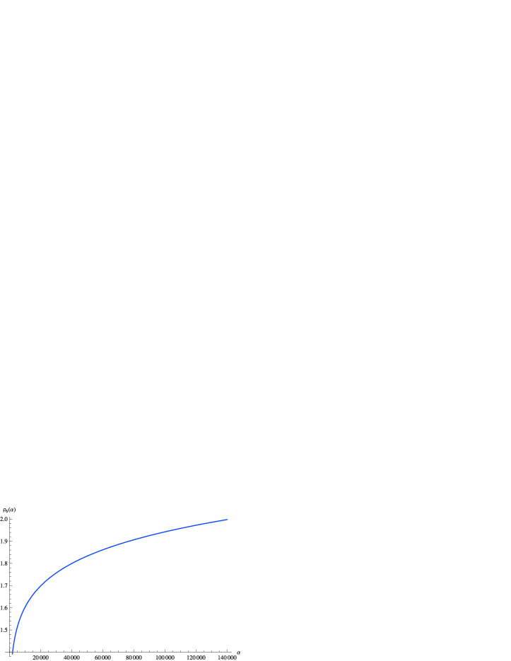
Figure 1: The graph of $\,\rho_{6}(\alpha)<2\,$.

3. Another interesting observation, concerning the coefficients of $\,R_{n}\,$ inspires the following

Conjecture 4.2.

For every fixed $\,k\in\mathbb{N}\,$, the coefficient $\,b_{k,n}\,$, $\,n>k\,$, of the polynomial

$$\,R_{n}(x)=x^{n}-b_{1,n}\,x^{n-1}+b_{2,n}\,x^{n-2}-\cdots+(-1)^{n}\,b_{n,n}\,,$$

satisfies

$$b_{k,n}=\frac{n^{2k}}{2^{k}\,k!(\alpha+1)\cdots(\alpha+2k-1)}+{\cal O}(n^{2k-1})\,.$$ (4.1)

Conjecture 4.2 is verified with our computer algebra approach for $\,1\leq k\leq 6\,$, but so far we do not have a proof for the general case. Having (4.1) proved, we could try to find the explicit form of $\,d_{k}\,$, the coefficient of $\,n^{2k}\,$ in Newton’s function $\,p_{k}(R_{n})\,$, and consequently to obtain two sequences $\{\ell_{k}\}\,$ and $\,\{u_{k}\}\,$ defined by $\,\ell_{k}=\sqrt{d_{k}/d_{k-1}}\,$ and $\,u_{k}=\sqrt[2k]{d_{k}}\,$ which tend monotonically from below and from above, respectively, to $\,c(\alpha)\,$, the sharp asymptotic Markov constant.

Acknowledgement. The authors are supported by the Bulgarian National Research Fund under Contract DN 02/14 and by the Sofia University Research Fund under Contract 80.10-11/2017.

Geno Nikolov,   Rumen Uluchev
Department of Mathematics and Informatics
University of Sofia
5 James Bourchier Blvd.
1164 Sofia
BULGARIA
E-mails:  geno@fmi.uni-sofia.bg,   rumenu@fmi.uni-sofia.bg

References

- [1] Aleksov, D., Nikolov, G.: Markov inequality with the Gegenbauer weight. J. Approx. Theory, 225, 2018, 224–241, https://doi.org/10.1016/j.jat.2017.10.008.
- [2] Dörfler, P.: Über die bestmögliche Konstante in Markov-Ungleichungen mit Laguerre Gewicht. Österreich. Akad. Wiss. Math.-Natur. Kl. Sitzungsber. II, 200, 1991, 13–20.
- [3] Dörfler, P.: Asymptotics of the best constant in a certain Markov-type inequality. J. Approx. Theory, 114, 2002, 84–97.
- [4] Mead, D. G.: Newton Identities. Amer. Math. Monthly 99, 1992, 749–751.
- [5] Nikolov, G., Shadrin, A.: On the Markov inequality with Laguerre weight. In: Progress in Approximation Theory and Applicable Complex Analysis, (N. K. Govil et al., eds.), Springer Optimization and Its Applications 117, 2017, pp. 1–17. DOI: 10.1007/978-3-319-49242-1_1.
- [6] Nikolov, G., Shadrin, A.: On the Markov inequality in the norm with the Gegenbauer weight. Constr. Approx., 2017, to appear. Also availabe as: arXiv:1701.07682v1 [math.CA].
- [7] Nikolov, G., Shadrin, A.: Markov –inequality with the Laguerre weight. In: Constructive Theory of Functions, Sozopol 2016, (K. Ivanov et al., eds.), Prof. Marin Drinov Publishing House, Sofia, 2017, to appear. Also availabe as: arXiv:1705.03824v1 [math.CA]
- [8] Szegő, G.: Orthogonal polynomials, AMS Colloq. Publ. 23, AMS, Providence, RI, 1975.
- [9] Turán, P.: Remark on a theorem of Ehrhard Schmidt. Mathematica (Cluj), 2, 1960, 373–378.
- [10] Van der Waerden, B. L.: Modern Algebra, Vol. 1, New York, Frederick Ungar Publishing Co., 1949.