Blocking and invasion for reaction-diffusion equations in periodic media

Abstract

We investigate the large time behavior of solutions of reaction-diffusion equations with general reaction terms in periodic media. We first derive some conditions which guarantee that solutions with compactly supported initial data invade the domain. In particular, we relate such solutions with front-like solutions such as pulsating traveling fronts. Next, we focus on the homogeneous equation set in a domain with periodic holes, and specifically in the cases where fronts are not known to exist. We show how the geometry of the domain can block or allow invasion. We finally exhibit a periodic domain on which the propagation takes place in an asymmetric fashion, in the sense that the invasion occurs in a direction but is blocked in the opposite one.

Keywords: reaction-diffusion equations, invasion, propagation, spreading, domains with holes.
MSC: 35A08, 35B30, 35K05, 35K57, 35B40

1 Introduction

1.1 Large time behavior for the Cauchy problem

Reaction-diffusion equations classically arise in the study of biological phenomena (propagation of genes, epidemics), in physics (combustion) and more recently in social sciences (rioting models). They have been extensively studied since the seminal papers of Fisher [13] and Kolmogorov, Petrovski and Piskunov [19] who dealt with the homogeneous equation

$$\partial_{t}u=\Delta u+f(u),\quad t>0,\ x\in\mathbb{R}^{N}.$$ (1.1)

A crucial progress in the study of (1.1) is due to Aronson and Weinberger [1]. The basic assumption there is that $f(0)=f(1)=0$. Then the authors consider three different sets of hypotheses. With the terminology commonly employed in the literature, they are:  monostable

$f>0\quad\text{in }(0,1)$;

$\exists\theta\in(0,1),\quad f=0\quad\text{in }[0,\theta],\quad f>0\quad\text{in }(\theta,1)$;

$\exists\theta\in(0,1),\quad f<0\quad\text{in }(0,\theta),\quad f>0\quad\text{in }(\theta,1)$.

The monostable case is the one considered in [13], [19] and includes the logistic equation $f(u)=u(1-u)$; the prototype of the bistable term is $f(u)=u(1-u)(u-\theta)$, which reduces to the Allen-Cahn nonlinearity when $\theta=1/2$.

Two key features of the equation (1.1) are exhibited in [19, 1]. First, the existence of a special type of solutions named traveling fronts (or traveling waves). These are solutions of the form $u(t,x)=\phi(x\cdot e-ct)$, with $e$ on the unit sphere $\mathbb{S}^{N-1}$, $c\in\mathbb{R}$ and $\phi(z)\to 1$ as $z$ goes to $-\infty$ and $\phi(z)\to 0$ as $z$ goes to $+\infty$. The second feature is the invasion property: for any “large enough” compactly supported non-negative initial datum, the solution of (1.1) converges locally uniformly to $1$ as time goes to infinity. This result requires the hypothesis $\int_{0}^{1}f>0$, which is automatically fulfilled in the monostable and combustion cases. How large the initial datum needs to be depends on the type of nonlinearity: in the monostable case it is sufficient to be larger than a positive constant on a large ball, in the combustion or bistable case the constant needs to be larger than $\theta$. Actually, in the monostable case, there exists a critical exponent $\beta>1$ such that if $f(u)\geq u^{\beta}$ for $u\sim 0$ (hence in particular if $f^{\prime}(0)>0$) then all solutions with non-negative, not identically equal to $0$ initial data converge to $1$ as $t$ goes to $+\infty$. This is known as the hair-trigger effect, c.f. [1]. Observe instead that in the combustion case, if the initial datum lies below $\theta$, then (1.1) reduces to the heat equation and thus the solution converges uniformly to $0$ as $t$ goes to $+\infty$. In the bistable case the situation is even worse; moreover if $\int_{0}^{1}f=0$ then all solutions with compactly supported initial data $\leq 1$ stay bounded away from $1$, and they all converge to $0$ if $\int_{0}^{1}f<0$.

The aim of this paper is to investigate the question of invasion for reaction-diffusion equations in periodic media. Specifically, we consider the problem

$$\begin{cases}\partial_{t}u=\nabla\cdot(A(x)\nabla u)+q(x)\cdot\nabla u+f(x,u),&t>0,\ x\in\Omega\\ \nu\cdot A(x)\nabla u=0,&t>0,\ x\in\partial\Omega.\end{cases}$$ (1.2)

combined with a nonnegative initial datum $u_{0}$ . Here $\Omega\subset\mathbb{R}^{N}$ is an unbounded smooth domain which is periodic in the directions of the canonical basis. Typical examples are domains with “holes” which are periodically arranged, that is, $\Omega=\left(K+L\mathbb{Z}^{N}\right)^{c}$ (here and in the sequel, for a given subset $A$ of $\mathbb{R}^{N}$, we denote its complement by $A^{c}:=\mathbb{R}^{N}\setminus A$) where $K\subset\mathbb{R}^{N}$ is a compact set and $L>0$. In the case $\Omega=\mathbb{R}^{N}$, we neglect the second equation in (1.2). The diffusion matrix $A$, the drift term $q$ and the nonlinearity $f$ are also assumed to be periodic with respect to the $x$ variable, with the same period as $\Omega$.

We shall describe the large time behavior of solutions in terms of the following properties.

Definition 1.1.

We say that a solution $u$ satisfies the properties of  persistence

if  $\displaystyle\limsup_{t\to+\infty}\left(\sup_{x\in\Omega}u(t,x)\right)<1$;

if  $\displaystyle\liminf_{t\to+\infty}\Big{(}\min_{x\in K}u(t,x)\Big{)}>0$ for all compact $K\subset\overline{\Omega}$;

if  $u(t,x)\to 1$ as $t$ goes to $+\infty$, locally uniformly in $x\in\overline{\Omega}$.

Persistence is compatible with both blocking and invasion, whereas the latter two properties are mutually exclusive.

We shall say that a function $u:\Omega\mapsto[0,1]$ is front-like if

$$\exists e\in\mathbb{S}^{N-1},\quad\lim_{\genfrac{}{}{0.0pt}{}{x\cdot e\to-\infty}{x\in\Omega}}u(x)=1,\quad\lim_{\genfrac{}{}{0.0pt}{}{x\cdot e\to+\infty}{x\in\Omega}}u(x)=0.$$ (1.3)

The kind of questions we address here are:

• Does the validity of the invasion property for all  front-like data implies that the invasion property holds for some  compactly supported data ?

• Does the validity of the invasion property for a single  front-like datum implies that the invasion property holds for some  compactly supported data ?

We will show in Theorem 1.3 that the answer to the first question is yes, specifying also how “large” the compactly supported data need to be. Then we will provide a negative answer to the second question, see Remark 1 after Theorem 1.10.

1.2 Statement of the main results

Throughout the paper, $\Omega$ is a domain with $C^{3}$ boundary, $\nu:\partial\Omega\to\mathbb{S}^{N-1}$ denotes its exterior normal field and $\partial_{\nu}$ the associated directional derivative. We further assume $\Omega$ to be periodic, i.e., there are $L_{1},\dots,L_{N}>0$ such that

$$\forall k\in L_{1}\mathbb{Z}\times\cdots\times L_{N}\mathbb{Z},\quad\Omega+\{k\}=\Omega.$$

We let $\mathcal{C}$ denote the periodicity cell:

$$\mathcal{C}:=\overline{\Omega}\cap\prod_{i=1}^{N}[0,L_{i}).$$

We assume, unless otherwise stated, that the coefficients are also periodic with respect to $x$ with the same periodicity as $\Omega$, i.e.,

$$\forall k\in L_{1}\mathbb{Z}\times\cdots\times L_{N}\mathbb{Z},\ x\in\overline{\Omega},\quad A(x+k)=A(x),\quad q(x+k)=q(x),$$

$$\forall k\in L_{1}\mathbb{Z}\times\cdots\times L_{N}\mathbb{Z},\ x\in\overline{\Omega},\ s\in[0,1],\quad f(x+k,s)=f(x,s).$$

The following regularity and ellipticity hypotheses will always be understood in the paper: $A\in C^{3}(\overline{\Omega})$ is a symmetric, uniformly elliptic matrix field, $q\in C^{1,\alpha}(\overline{\Omega})$, for some $\alpha\in(0,1)$ is a vector field and $f:\overline{\Omega}\times[0,1]\mapsto\mathbb{R}$ is globally Lipschitz-continuous. We shall denote $0<\lambda\leq\Lambda$ the ellipticity constants of the matrix field $A$, so that

$$\forall x\in\overline{\Omega},\quad\lambda I_{N}\leq A(x)\leq\Lambda I_{N},$$ (1.4)

where $I_{N}$ is the identity matrix and the order is the usual one on symmetric matrices. We shall further assume that $f$ satisfies the following properties:

$$\forall x\in\overline{\Omega},\quad f(x,0)=f(x,1)=0,$$

$$\exists S\in(0,1)\ \text{such that}\ s\mapsto f(x,s)\text{ is strictly positive for all}\ x\in\overline{\Omega},\ s\in(S,1).$$

This means that $0$ and $1$ are steady states for (1.2), with $1$ being stable whereas $0$ could be both stable or unstable. We extend $f(x,s)$ by a negative function for $s\not\in[0,1]$ such that the resulting function is globally Lipschitz-continuous. The above properties allow us to define

$$\theta:=\max\left\{s\in[0,1)\ :\ \exists x\in\overline{\Omega},\ f(x,s)=0\right\}.$$ (1.5)

Namely, $\theta\in[0,1)$ is the smallest value for which $f>0$ in $\overline{\Omega}\times(\theta,1)$.

This paper deals with the phenomena of invasion, persistence and blocking - formulated in Definition 1.1 - for equation (1.2), and is divided into two main parts. In the first part, we give sufficient conditions for persistence and invasion to occur for “large enough” compactly supported initial data. In the second part, we study how the geometry of the domain $\Omega$ can influence the invasion in the bistable case.

1.2.1 Persistence and invasion

Our first result provides a sufficient condition for the persistence of solutions to (1.2) with “large enough” initial data, in the absence of the drift term $q$.

Theorem 1.2.

Assume that $q\equiv 0$ and that $f$ satisfies

$$\int_{\mathcal{C}}\int_{0}^{1}f(x,s)\,ds\,dx>0.$$ (1.6)

Then, for all $\eta\in(\theta,1)$, where $\theta$ is defined by (1.5), there is $r>0$ such that the persistence property holds for every solution to (1.2) arising from a non-negative initial datum satisfying

$$u_{0}>\eta\quad\text{ in }\ \Omega\cap B_{r}.$$

Let us make one comment about the condition $q\equiv 0$. It comes from the fact that our proof of Theorem 1.2 relies on an energy method. This condition is presumably not optimal, but it guarantees some control on the drift: indeed, a drift that is “too strong” would lead to extinction for all compactly supported initial data, no matter how large they are.

Our second main result is the equivalence of the invasion property for initial data which are “large enough on a large set” and for front-like initial data, i.e., satisfying (1.3).

Theorem 1.3.

The following properties are equivalent:

1. Invasion occurs for all solutions of (1.2) with non-negative front-like initial data.

2. Invasion occurs for “large enough” initial data, in the sense that for all $\eta\in(\theta,1)$, where $\theta$ is defined by (1.5), there is $r>0$ such that the invasion property holds for every solution to (1.2) arising from a non-negative initial datum satisfying

   $$u_{0}>\eta\quad\text{ in }\ \Omega\cap B_{r}.$$

The fact that $(ii)$ implies $(i)$ in Theorem 1.3 is an immediate consequence of the parabolic comparison principle. The interest is in the the other implication. We mention that a related result is contained in the work [27] by Weinberger. However, the hypotheses there are more restrictive than our condition $(i)$ in Theorem 1.3: first, compared with our definition (1.3), front-like data in [27] are assumed to be strictly smaller than $1$, second, the emerging solutions need to have a positive spreading speed rather than just satisfy the invasion property. The method of [27] relies on a discrete dynamical system approach. In particular, the rather involved argument that allows the author to handle compactly supported initial data cannot be directly performed in the continuous PDE setting.

As already mentioned, it may be complicated to check that condition $(i)$ of Theorem 1.3 holds. Our next result – Theorem 1.5 – provides a sufficient condition for the invasion property expressed in terms of pulsating traveling fronts. These are particular entire solutions of (1.2) satisfying some structural properties that generalize to the periodic framework the notion of traveling front. They were first introduced in dimension $N=1$ by Shigesada, Kawasaki and Teramoto in [24].

Definition 1.4.

A pulsating traveling front in the direction $e\in\mathbb{S}^{N-1}$ with speed $c\in\mathbb{R}\backslash\{0\}$ connecting $1$ to $0$ is an entire (i.e., for all times) solution of (1.2) $0<v<1$ such that

$$\begin{cases}\forall z\in\displaystyle\prod_{i=1}^{N}L_{i}\mathbb{Z},\ x\in\Omega,\quad v(t+\frac{z\cdot e}{c},x)=v(t,x-z)\\ v(t,x)\underset{x\cdot e\to-\infty}{\longrightarrow}1\ \text{ and }\ v(t,x)\underset{x\cdot e\to+\infty}{\longrightarrow}0.\end{cases}$$ (1.7)

A pulsating traveling front with speed $c=0$ is a front-like stationary solution of (1.2), in the sense of (1.3).

Observe that, if $v$ is a pulsating traveling front, then $x\mapsto v(t,x)$ is front-like for all $t\in\mathbb{R}$. The use of traveling fronts to study the large time behavior of solutions of the Cauchy problem in the combustion and bistable cases is quite a natural approach, already used in the pioneering paper [1] for the homogeneous equation (1.1). For later use, we introduce the following:

Hypothesis 1.

For every direction $e\in\mathbb{S}^{N-1}$, there is a pulsating traveling front with speed $c>0$.

The requirement that the speeds of the fronts are positive in Hypothesis 1 is necessary for the invasion property to hold, in the sense that, owing to the parabolic comparison principle, the existence of – even a single – pulsating traveling front with speed $c\leq 0$ prevents the invasion of all solutions with compactly supported initial data smaller than $1$.

Theorem 1.5.

Assume that there is $\delta>0$ such that

$$s\mapsto f(x,s)\text{ is nonincreasing on $(0,\delta)$ and on $(1-\delta,1)$}.$$

Then, Hypothesis 1 implies that properties $(i)$-$(ii)$ of Theorem 1.3 hold.

The usefulness of this result lies in the fact that there is a huge literature about pulsating traveling fronts. In particular, their existence and the positivity of their speed is proved by Berestycki and Hamel in [3, Theorems 1.13 , 1.14] when $f$ is of the monostable or combustion type (cf. the definition given in Section 1.1 in the homogeneous case) under the following additional assumptions on $q$:

$$\begin{cases}\nabla\cdot q=0\quad&\text{in }\overline{\Omega},\\ \int_{\mathcal{C}}q=0,\\ q\cdot\nu=0\quad&\text{on }\partial\Omega.\end{cases}$$ (1.8)

Observe that in the monostable case the monotonicity hypothesis of Theorem 1.5 is not fulfilled, but since the larger the nonlinearity, the more likely the invasion property holds, the idea is to consider a term $\tilde{f}\leq f$ of combustion type. This allows to derive the following result concerning non-negative reaction terms, such as monostable and combustion.

Corollary 1.6.

Assume that $q$ satisfies (1.8) and that $f$ satisfies

$$\forall x\in\Omega,\ \forall s\in(0,1),\quad f(x,s)\geq 0.$$ (1.9)

Then, properties $(i)$-$(ii)$ of Theorem 1.3 hold.

We point out that Corollary 1.6 could be also derived by combining the results of [3] with those of Weinberger [27] mentioned before.

Under the generality of our assumptions on $f$, which include the bistable case, the question of the existence of fronts is still widely open, in particular if the domain $\Omega$ is not $\mathbb{R}^{N}$. We are not aware of any result in such case. If the equation is set on $\mathbb{R}^{N}$, then Xin [30, 29] and Ducrot [11] derive the existence of fronts with positive speed under some conditions on the coefficients. Theorem 1.5 then yields the invasion result in such cases, see Corollaries 3.3, 3.4 below.

One may wonder whether Hypothesis 1 is necessary in Theorem 1.5. This is not the case. Indeed Zlatoš exhibits in [31] a bistable periodic nonlinearity such that the $1$-dimensional equation

$$\partial_{t}u=\partial_{xx}u+f(x,u),\quad t>0,\ x\in\mathbb{R},$$

admits no pulsating traveling fronts (actually, he shows that there are no transition fronts, a notion generalizing pulsating traveling fronts), but such that the invasion property holds for sufficiently large compactly supported initial data. On the other hand, we exhibit in Theorem 1.9 below a situation where there are no fronts and invasion does not occur. We mention that other examples of reaction-diffusion equations that do not admit fronts are known in dimension $1$, see [28], and in cylindrical domains (with a drift-term), see [4].

Once we know that invasion occurs for a solution with compactly supported initial datum smaller than $1$, it is not hard to see that this happens with a strictly positive speed, see Remark 2 below. In all the situations where Hypothesis 1 holds, we can actually characterize this speed through an analogous formula to the one derived by Freidlin and Gärtner in [15, 14] in the KPP case. This was first proved by the second author in [23] when $\Omega=\mathbb{R}^{N}$ and then by the first author in [10] for periodic domains. We mention that Weinberger also derives a similar formula in [27].

Our next result applies to equations with non-negatives nonlinearities – such as monostable or combustion – set in the whole space. It provides an explicit sufficient condition for invasion to occur, as well as a lower bound on the asymptotic speed at which this takes place. This is expressed in terms of the following quantity:

$$R(f):=\sup_{0<K<H<1}\bigg{(}(H-K)\min_{\begin{subarray}{c}x\in\overline{\Omega}\\ s\in[K,H]\end{subarray}}f(x,s)\bigg{)},$$

which is the area of the largest rectangle one can fit under the graph of $s\mapsto\inf_{x\in\overline{\Omega}}f(x,s)$ in the upper half-plane. For this result, it is convenient to consider equations in non-divergence form, that is,

$$\partial_{t}u=Tr(A(x)D^{2}u)+q(x)\cdot\nabla u+f(x,u),\quad\forall t>0,\ \forall x\in\mathbb{R}^{N},$$ (1.10)

under the usual standing assumption of Section 1.2 on the terms $A$, $q$, $f$.

Theorem 1.7.

Assume that $f$ satisfies (1.9) and that $q$ is continuous and satisfies

$$\limsup_{|x|\to+\infty}\,q(x)\cdot\frac{x}{|x|}<\frac{\lambda}{\sqrt{\Lambda}}\sqrt{R(f)},$$

where $\lambda,\Lambda$ are given by (1.4). Then, properties $(i)$-$(ii)$ of Theorem 1.3 hold for the equation (1.10).

Moreover, calling $w^{\star}:=\frac{\lambda}{\sqrt{\Lambda}}\sqrt{R(f)}-\limsup_{|x|\to+\infty}q(x)\cdot\frac{x}{|x|}$, there holds

$$\forall c<w^{\star},\quad\inf_{|x|\leq ct}u(t,x)\underset{t\to+\infty}{\longrightarrow}1.$$

Let us state make some comments about this result. First, we point out that it holds without any assumption on $q$ besides boundedness, unlike Corollary 1.6 which requires (1.8). Next, the theorem holds true without the periodicity assumption, provided (1.9) is fulfilled by the function $\inf_{x\in\mathbb{R}^{N}}f(x,\cdot)$. This is a non-degeneracy hypothesis, without which the result could not hold (if $f(x,\cdot)\equiv 0$ for $x$ large for instance, there is no way invasion could occur). The proof will actually use only this non-degeneracy hypothesis, which is guaranteed by the periodicity. Finally, one can observe that the more negative $q(x)\cdot\frac{x}{|x|}$ is, the larger $w^{\star}$ becomes. This is a bit counter-intuitive because $q(x)\cdot\frac{x}{|x|}<0$ roughly means that the drift “gathers the mass” instead of scattering it. Hence, such a drift should slow down the invasion. This suggests that our bound $w^{\star}$ on the invasion speed may not be optimal in general. On the other hand, because this drift prevents the mass to scatter, it is natural that the more negative $q(x)\cdot\frac{x}{|x|}$ is, the more likely invasion should occur. In any case, though probably not optimal, our estimate on the invasion speed has the advantage of being explicit and easy to compute. While an estimate in the same spirit is derived in [7] under the assumption $\partial_{s}f(\cdot,0)>0$, we are not aware of analogous results of this type in the combustion case.

The proof of Theorem 1.2 is carried out in Section 2. Theorem 1.3 and Theorem 1.5 are derived in Section 3. In Section 3.2, we derive Corollary 1.6. Theorem 1.7 is proved in Section 4.

1.2.2 Influence of the geometry of the domain

The results presented above provide some sufficient conditions ensuring the persistence or invasion properties. It is known that, if $f$ is of the bistable type, the geometry of the domain can produce “obstacles” which may prevent propagation. This is observed by Berestycki, Hamel and Matano in [5] for an exterior domain (i.e., the complement of a compact set) and by Berestycki, Bouhours and Chapuisat in [2] for a cylindrical-type domain with a bottleneck. If such obstacles repeat periodically in the domain, one could expect that the blocking property holds. We will show that this is indeed the case, but also that other scenarios are possible.

We consider the simplest problem set in a periodic domain:

$$\begin{cases}\partial_{t}u=\Delta u+f(u),&t>0,\ x\in\Omega\\ \partial_{\nu}u=0,&t>0,\ x\in\partial\Omega,\end{cases}$$ (1.11)

where $f$ is an unbalanced bistable nonlinearity, i.e.,

$$\exists\theta\in(0,1),\quad f<0\quad\text{in }(0,\theta),\quad f>0\quad\text{in }(\theta,1),\quad\int_{0}^{1}f(s)ds>0.$$ (1.12)

Notice that, under the assumption (1.12), Theorem 1.2 ensures that the persistence property for “large enough” initial data holds for problem (1.11), whatever the domain $\Omega$ is. However, we will see that the geometry of $\Omega$ affects the way this persistence takes place, in three radically different ways. Namely, we construct three periodic domains $\Omega_{1}$, $\Omega_{2}$, $\Omega_{3}$ that exhibit, respectively, invasion, blocking (in the sense of Definition 1.1) and a new phenomenon that we call oriented invasion. Let us mention that our results could be carried out for the more general equation (1.2), but we have chosen to emphasize here the role of the geometry of the domain.

The domain $\Omega_{1}$ is given by the whole space with a star-shaped hole $K$ repeated periodically, with a period $L$ sufficiently large.

Theorem 1.8.

Let $f$ satisfy (1.12) and let $K\subset\mathbb{R}^{N}$ be a star-shaped compact set. Then, for $L>0$ sufficiently large, properties $(i)$-$(ii)$ of Theorem 1.3 hold for the problem (1.11) set on

$$\Omega_{1}:=\left(K+L\mathbb{Z}^{N}\right)^{c}.$$

Next, building on the result of [5], we exhibit a domain $\Omega_{2}$ where the propagation is always blocked.

Theorem 1.9.

Let $f$ satisfy (1.12). There exists a periodic domain $\Omega_{2}$ such that, for the problem (1.11) set on $\Omega_{2}$, the following hold:

1. Any solution arising from a compactly supported initial datum $u_{0}\leq 1$ is blocked in the sense of Definition 1.1.

2. There exists a solution with compactly supported initial datum which converges (increasingly) to a periodic non-constant stationary solution as $t$ goes to $+\infty$.

3. Invasion fails for every front-like initial datum and moreover there exist no pulsating traveling fronts.

The failure of the invasion property is in strong contrast with the homogeneous case $\Omega=\mathbb{R}^{N}$, where such property is guaranteed by the condition $\int_{0}^{1}f(s)ds>0$, at least for large enough initial data. We point out that Theorem 1.9 part $(ii)$ implies the existence of an intermediate periodic steady state between $0$ and $1$ which is stable from below. So, it turns out that the geometry of $\Omega_{2}$ alters the bistable character of the nonlinearity $f$ making some non-trivial stable steady states appear. This is the reason why there are no fronts in such case, but one should rather expect the existence of propagating terraces instead, see [11, 18].

We finally construct a domain $\Omega_{3}$ which exhibits a new phenomenon that we call oriented invasion. Namely, invasion occurs in a direction $e$, with a positive linear speed, whereas the propagation is blocked in the opposite direction $-e$. We state and prove the theorem in $\mathbb{R}^{2}$, but it can be easily generalized to higher dimensions. We let $(e_{1},e_{2})$ denote the unit vectors of the canonical basis of $\mathbb{R}^{2}$.

Theorem 1.10.

Let $f$ satisfy (1.12). There exists a periodic domain $\Omega_{3}\subset\mathbb{R}^{2}$ and a positive constant $c$ such that, for every $\eta>\theta$, there is $r>0$ for which the following properties hold for every solution to (1.11) arising from a compactly supported initial datum satisfying

$$0\leq u_{0}\leq 1,\qquad u_{0}>\eta\quad\text{ in }\ \Omega\cap B_{r}.$$

1. Invasion in the direction $e_{1}$:

   $$\forall 0<c_{1}<c_{2}<c,\ \forall a>0,\quad\min_{\begin{subarray}{c}x\in\overline{\Omega}_{3}\\ c_{1}t\leq x\cdot e_{1}\leq c_{2}t\\ |x\cdot e_{2}|\leq a\end{subarray}}|u(t,x)-1|\underset{t\to+\infty}{\longrightarrow}0.$$

2. Blocking in the direction $-e_{1}$:

   $$u(t,x)\underset{x\cdot e_{1}\to-\infty}{\longrightarrow}0\quad\text{uniformly in }t>0.$$

Theorem 1.10 provides an example of a periodic domain on which invasion takes place in an asymmetric way. In the KPP case, it turns out that the speed of invasion in a given direction and in the opposite one do coincide. Our result provides a counter-example to this fact in the bistable case.

Remark 1.

From statement $(i)$ of Theorem 1.10, it is easy to deduce that the invasion property is verified for any initial datum which is front-like in the direction $e_{1}$, i.e., satisfying (1.3) with $e=e_{1}$. This shows that the invasion property for a single front-like initial datum does not suffice to guarantee that invasion occurs for “large enough” compactly supported data. Namely, in Theorem 1.3, one cannot weaken property $(i)$ by the existence of one single front-like initial datum for which invasion occurs. The possible extension of the theorem would be by assuming that in any direction there is a front-like initial datum for which invasion occurs. We leave it as an open question.

The proofs of Theorems 1.8 and 1.9 are given in Sections 5.1 and 5.2 respectively. Section 6 is dedicated to the proof of Theorem 1.10.

2 Persistence

This section is devoted to the proof of the persistence result, Theorem 1.2. In this whole section, we assume that $q\equiv 0$ and that $f$ satisfies (1.6). The proof relies on the study of the stationary problem

$$\begin{cases}\nabla\cdot(A(x)\nabla u)+f(x,u)=0,&x\in\Omega\\ \nu\cdot A(x)\nabla u=0,&x\in\partial\Omega.\end{cases}$$ (2.13)

The main tool is the construction of a family of solutions in truncated domains. This will be achieved using an energy method, in the same spirit of Berestycki, Lions [8], where the authors study the existence of positive solutions for homogeneous bistable equations in the whole space $\mathbb{R}^{N}$.

We consider the primitive of $f$, defined by

$$F(x,s):=\int_{0}^{s}f(x,\sigma)d\sigma.$$

For $r>0$, we introduce the energy functional $\mathcal{E}_{r}$ associated with (2.13) in the truncated domain $\Omega\cap B_{r}$:

$$\mathcal{E}_{r}(\phi):=\int_{\Omega\cap B_{r}}\left(\frac{1}{2}(A(x)\nabla\phi,\nabla\phi)-F(x,\phi)\right),$$

acting on the space $H^{1}_{0}(\overline{\Omega}\cap B_{r})$. We study the existence of minimizers for this energy. In order to do so, we first derive a geometrical lemma ensuring that $\Omega$ and $B_{r}$ are not tangent for a.e. $r>0$. We recall that $\nu(x)$ stands for the exterior normal derivative at point $x\in\partial\Omega$.

Lemma 2.1.

For a.e. $r>0$, there holds

$$\forall x\in(\partial\Omega)\cap\partial B_{r},\quad\nu(x)\neq\pm\frac{x}{|x|}.$$ (2.14)

Proof.

Let $d$ be a regularised signed distance from $\partial\Omega$, that is, a smooth function on $\mathbb{R}^{N}$ coinciding with the signed distance from $\partial\Omega$ in a neighbourhood of $\partial\Omega$, positive inside $\Omega$. Consider the pair of functions

$$\rho_{\pm}(x):=|x|\pm d(x).$$

This functions are smooth outside the origin. It follows from the Morse-Sard theorem [22] that the inverse images $\rho_{\pm}^{-1}(r)$ do not contain any critical points of $\rho_{\pm}$, except for $r$ belonging respectively to some sets $\mathcal{R}_{\pm}$ with zero Lebesgue measure. Hence, for $r\in\mathbb{R}^{+}\setminus(\mathcal{R}_{-}\cup\mathcal{R}_{+})$, that is, for a.e. $r>0$, any $x\in\partial\Omega\cap\partial B_{r}$ satisfies $\rho_{\pm}(x)=|x|=r$ and thus, for such $x$, we have

$$0\neq\nabla\rho_{\pm}(x)=\frac{x}{|x|}\mp\nu(x).$$

∎

For all $r$ for which (2.14) holds, the set $\Omega\cap B_{r}$ satisfies an interior and exterior cone condition. Also, it is not hard to check that, for all $r$ for which (2.14) holds, the set $\Omega\cap B_{r}$ has a finite number of connected components

Proposition 2.2.

For all $r>0$ such that (2.14) holds, the functional $\mathcal{E}_{r}$ admits a global minimiser $\underline{u}_{r}\in H^{1}_{0}(\overline{\Omega}\cap B_{r})$ such that $0\leq\underline{u}_{r}\leq 1$ a.e. in $\Omega\cap B_{r}$.

Proof.

First, observe that, because we have extended $f(x,s)$ by a negative function for $s>1$, we have

$$\forall x\in\overline{\Omega},\ \forall s\geq 0,\quad F(x,s)\leq\int_{0}^{\min\{s,1\}}f(x,\sigma)d\sigma\leq\max_{\overline{\Omega}\times[0,1]}f.$$

We deduce that

$$\mathcal{E}_{r}\geq-\max_{\overline{\Omega}\times[0,1]}f|B_{r}|,$$

that is, $\mathcal{E}_{r}$ is bounded from below. Consider a minimizing sequence $(u_{n})_{n\in\mathbb{N}}$ of elements of $H_{0}^{1}(\overline{\Omega}\cap B_{r})$. We can assume without loss of generality that $\operatorname*{ess\,sup}u_{n}\leq 1$, because, defining $v_{n}=\min(u_{n},1)$, we have that $v_{n}\in H^{1}_{0}(\overline{\Omega}\cap B_{r})$ and $\mathcal{E}_{r}(v_{n})\leq\mathcal{E}_{r}(u_{n})$ again because $f(x,s)<0$ for $s>1$. Likewise, we can take $\operatorname*{ess{\,}inf}u_{n}\geq 0$. Let us check that the sequence $(u_{n})_{n\in\mathbb{N}}$ is bounded in $H^{1}(\Omega\cap B_{r})$. Indeed, on the one hand, the sequence is bounded in $L^{2}(\Omega\cap B_{r})$, and on the other hand, remembering that $\lambda$ denotes the ellipticity constant of $A$,

$$\frac{1}{2}\lambda\|\nabla u_{n}\|^{2}_{L^{2}(\Omega\cap B_{r})}-\max_{\overline{\Omega}\times[0,1]}f|B_{r}|\leq\mathcal{E}_{r}(u_{n}).$$

Now, we cannot directly apply the Rellich-Kondrachov theorem to the sequence $(u_{n})_{n\in\mathbb{N}}$ because $\Omega\cap B_{r}$ is not necessarily smooth. However, it is a Lipschitz domain thanks to (2.14), hence we can apply the usual Sobolev extension theorem (see [26, Section 6] or [9]) for $(u_{n})_{n\in\mathbb{N}}$ and then apply the Rellich-Kondrachov theorem to the sequence of extended functions, getting then that, up to extraction, $(u_{n})_{n\in\mathbb{N}}$ converges in the $L^{2}$ norm (up to subsequences) to some $u\in L^{2}(\Omega\cap B_{r})$.

Let us show that the convergence actually holds in $H_{0}^{1}(\overline{\Omega}\cap B_{r})$. To do so, we show that $(u_{n})_{n\in\mathbb{N}}$ is a Cauchy sequence in this space. For $m,n\in\mathbb{N}$, we have

$$\begin{array}[]{rl}\inf_{H^{1}_{0}(\overline{\Omega}\cap B_{r})}\mathcal{E}_{r}&\leq\mathcal{E}_{r}\Big{(}\frac{u_{m}+u_{n}}{2}\Big{)}\\ &\leq\frac{1}{2}\mathcal{E}_{r}(u_{m})+\frac{1}{2}\mathcal{E}_{r}(u_{n})-\frac{\lambda}{4}\|\nabla(u_{n}-u_{m})\|^{2}_{L^{2}(\Omega\cap B_{r})}\\ &\quad+\frac{1}{2}\int_{\Omega\cap B_{r}}\Big{(}F(x,u_{m})+F(x,u_{n})-2F\Big{(}x,\frac{u_{m}+u_{n}}{2}\Big{)}\Big{)}.\end{array}$$

Using the fact that $s\mapsto F(x,s)$ is Lipschitz-continuous, uniformly in $x$, and that $(u_{n})_{n\in\mathbb{N}}$ is a Cauchy sequence in $L^{2}(\Omega\cap B_{r})$, and therefore in $L^{1}(\Omega\cap B_{r})$, we see that the above integral goes to $0$ as $m,n$ go to $+\infty$. On the other hand, $\frac{1}{2}\mathcal{E}_{r}(u_{m})+\frac{1}{2}\mathcal{E}_{r}(u_{m})\to\inf_{H^{1}_{0}(\overline{\Omega}\cap B_{r})}\mathcal{E}_{r}$ as $m,n$ go to $+\infty$. It follows that $(\nabla u_{n})_{n\in\mathbb{N}}$ is a Cauchy sequence in $L^{2}(\Omega\cap B_{r})$. Now, by continuity of $\mathcal{E}_{r}$ in $H^{1}_{0}(\overline{\Omega}\cap B_{r})$, we conclude that the limit $u$ is a global minimiser for $\mathcal{E}_{r}$. Finall, the fact that $0\leq u\leq 1$ a.e. follows from the same argument as before. ∎

We know that $\underline{u}_{r}$ satisfies the Euler-Lagrange equation associated with $\mathcal{E}_{r}$, together with mixed boundary conditions. Namely, it is a solution of the problem (2.13) inside $B_{r}$ and vanishes on $\Omega\cap\partial B_{r}$ in the sense of the trace. However, at this stage, we cannot exclude that the minimizer $\underline{u}_{r}$ is the trivial solution identically equal to zero. Owing to Lemma 2.1, we can infer that $\underline{u}_{r}$ is continuous on $\overline{\Omega\cap B_{r}}$, as shown in the following.

Lemma 2.3.

If (2.14) holds then $\underline{u}_{r}\in C^{0}(\overline{\Omega\cap B_{r}})$ and $\max_{\overline{\Omega\cap B_{r}}}\underline{u}_{r}<1$.

Proof.

Let $r$ be such that (2.14) holds. Then, the weak bounded solution $\underline{u}_{r}$ is actually continuous up to the boundary of $\Omega\cap B_{r}$, see [25, Theorem 14.5]. Because $\underline{u}_{r}$ is continuous and vanishes on $\Omega\cap\partial B_{r}$, it attains its maximum $M\leq 1$ at some $\bar{x}\in\overline{\Omega}\cap B_{r}$. Assume by contradiction that $M=1$. The function $v:=M-\underline{u}_{r}$ is non-negative, vanishes at $\bar{x}$ and satisfies $\nabla(A(x)\nabla v)=f(x,M-v)$ in $\Omega\cap B_{r}$. Because $s\mapsto f(x,s)$ is Lipschitz-continuous uniformly in $x$, we see that $\nabla\cdot(A(x)\nabla v)=f(x,M-v)$ can be rewritten as a linear equation with bounded coefficients. It follows from Hopf’s lemma and $\nu A\nabla v=0$ on $(\partial\Omega)\cap B_{r}$ that $\bar{x}\notin\partial\Omega$. Thus, the strong maximum principle implies that $v\equiv 0$ on the connected component $\mathcal{O}$ of $\Omega\cap B_{r}$ containing $\bar{x}$. Observe that $\overline{\mathcal{O}}\cap\partial B_{r}\neq\emptyset$ because $\Omega$ is connected. As a consequence, since $v$ is continuous up to the boundary, there exists $x\in\Omega\cap\partial B_{r}$ such that $v(x)=0$, i.e., $\underline{u}_{r}(x)=M$. We have reached a contradiction because $\underline{u}_{r}=0$ on $\Omega\cap\partial B_{r}$. ∎

The next lemma states that $\underline{u}_{r}\not\equiv 0$, provided $r>0$ is large enough. That is, we have built non-trivial solutions of (2.13) set on truncated domains.

Lemma 2.4.

Assume that $f$ satisfies (1.6). Then, there is $R^{\star}$ such that, for $r>R^{\star}$, there holds

$$\underline{u}_{r}\not\equiv 0.$$

Proof.

Since $\underline{u}_{r}$ minimises $\mathcal{E}_{r}$, we can get an upper bound for $\mathcal{E}_{r}(\underline{u}_{r})$ by estimating $\mathcal{E}_{r}(\phi_{r})$ on a suitable function $\phi_{r}\in H^{1}_{0}(\overline{\Omega}\cap B_{r})$. For $r>1$, we define $\phi_{r}:\overline{\Omega}\cap B_{r}\to\mathbb{R}$ as follows:

$$\phi_{r}(x)=\begin{cases}1&\text{if }|x|\leq r-1,\\ r-|x|&\text{if }r-1<|x|<r.\end{cases}$$

Observe that $|\nabla\phi_{r}|\leq 1$. We compute

$$\begin{split}\mathcal{E}_{r}(\phi_{r})&=\int_{\Omega\cap B_{r}}\left(\frac{1}{2}(A\nabla\phi_{r})\cdot\nabla\phi_{r}-F(x,\phi_{r})\right)\\ &\leq\frac{1}{2}\Lambda|B_{r}\setminus B_{r-1}|-\int_{\Omega\cap B_{r-1}}F(x,1)-\left(\min_{\overline{\Omega}\times[0,1]}F\right)|B_{r}\setminus B_{r-1}|,\end{split}$$

where $\Lambda$ is given by (1.4). We eventually infer the existence of a constant $C$ independent of $r$ such that

$$\forall r>1,\quad\mathcal{E}_{r}(\underline{u}_{r})\leq Cr^{N-1}-\int_{\Omega\cap B_{r-1}}F(x,1).$$

Observing that, for any measurable periodic function $g$ in $L^{1}_{loc}(\mathbb{R}^{N})$, we have $\fint_{B_{r}}g\to\fint_{[0,L_{1}]\times\ldots\times[0,L_{n}]}g$ as $r$ goes to $+\infty$, where $\fint$ stands for the integral average, we have

$$|\Omega\cap B_{r}|\sim_{r\to+\infty}\frac{|\mathcal{C}|}{\prod L_{i}}|B_{r}|=\frac{|\mathcal{C}|}{\prod L_{i}}|B_{1}|r^{N},$$

and then

$$\frac{1}{r^{N}}\int_{\Omega\cap B_{r-1}}F(x,1)\underset{r\to+\infty}{\longrightarrow}\frac{|\mathcal{C}|}{\prod L_{i}}|B_{1}|\fint_{\mathcal{C}}F(x,1).$$

Then, because the latter term is positive by hypothesis (1.6), we have

$$\limsup_{r\to+\infty}\frac{\mathcal{E}_{r}(\underline{u}_{r})}{r^{N}}\leq\limsup_{r\to+\infty}\left(C\frac{1}{r}-\frac{1}{r^{N}}\int_{\Omega\cap B_{r-1}}F(x,1)\right)<0,$$

whence $\mathcal{E}_{r}(\underline{u}_{r})<0$ if $r>0$ is sufficiently large. Therefore, $\underline{u}_{r}\not\equiv 0$ because $\mathcal{E}_{r}(0)=0$, and the result follows. ∎

Now, we can prove Theorem 1.2.

Proof of Theorem 1.2.

Thanks to Lemma 2.4, we can take $r>0$ such that $\underline{u}_{r}\not\equiv 0$. This function, extended by $0$ on $\Omega\backslash\overline{B}_{r}$, is a generalized subsolution of (1.2). Let $\underline{u}$ denote the solution of (1.2) arising from such initial datum. Using the parabolic comparison principle, it is classical to get that $\underline{u}(t,x)$ is increasing with respect to $t$ and converges locally uniformly in $\overline{\Omega}$ to a stationary solution of (1.2) as $t$ goes to $+\infty$. This stationary solution is strictly positive, thanks to the elliptic strong maximum principle and Hopf principle, and then $\underline{u}(t,x)$ satisfies the persistence property. By the parabolic comparison principle, we can infer that every solution of (1.2) with initial datum $u_{0}$ satisfying $u_{0}\geq\underline{u}_{r}$ satisfies the persistence property.

Next, take $\eta\in(\theta,1)$, and, for $n~\in\mathbb{N}$, let $u^{n}_{0}$ be a function with compact support in $\overline{\Omega}\cap B_{n}$ such that $u^{n}_{0}\leq\eta$ and

$$u_{0}^{n}=\eta\quad\text{ in }\ \overline{\Omega}\cap B_{n-1}.$$

Then, we have that $\nu\cdot(A(x)\nabla u^{n}_{0})=0,\ \forall x\in\partial\Omega\cap B_{n-1}$, i.e., $u_{0}^{n}$ satisfies there the boundary conditions of (1.2). This is necessary to have the usual parabolic estimates up to time $t=0$, see, for instance [20, Theorems 5.2, 5.3]. Let $u^{n}(t,x)$ denote the solution of (1.2) arising from the initial datum $u^{n}_{0}$. By the parabolic estimates, $u^{n}$ converges locally uniformly in $[0,+\infty)\times\overline{\Omega}$ to the solution $v$ of (1.2) with constant initial datum $v(0,\cdot)\equiv\eta$. Because $\eta>\theta$, $v(t,x)$ converges uniformly to $1$ as $t$ goes to $+\infty$ : indeed, we can define $z(t)$ to be the solution of the ODE $\dot{z}(t)=\min_{x\in\overline{\Omega}}f(x,z(t))$ with initial value $z(0)=\eta$. This is a subsolution of (1.2), whence the parabolic comparison principle yields $z(t)\leq v(t,x)$ for all $t\geq 0$, $x~\in\Omega$. Observe that $z(t)$ goes to $1$ as $t$ goes to $+\infty$, because $z(0)>\theta$ and $\theta$ is defined by (1.5) as the largest $s\in[0,1)$ such that $f(x,s)$ vanishes. Combining this with the fact that $v\leq 1$, we obtain the uniform convergence of $v(t,\cdot)$ to $1$ as $t$ goes to $+\infty$. Because $\underline{u}_{r}<1$ and is compactly supported in $\overline{\Omega\cap B_{r}}$, there exists $T>0$ such that $v(T,\cdot)>\underline{u}_{r}$. We can then find $\bar{n}$ so that

$$\forall x\in\overline{\Omega\cap B_{r}},\quad u^{\bar{n}}(T,x)\geq\underline{u}_{r}(x).$$

The parabolic comparison principle implies that $u^{\bar{n}}(T+t,\cdot)\geq\underline{u}(t,\cdot)$ and therefore $u^{\bar{n}}$ satisfies the persistence property. By comparison, the same holds true for any solution of (1.2) with initial datum $u_{0}$ larger than $u^{\bar{n}}_{0}$, and in particular if $u_{0}>\eta$ on $\overline{\Omega}\cap B_{\bar{n}}$, hence the result. ∎

Now that Theorem 1.2 is proved, and before turning to the proof of Theorem 1.3, we show that, under an additional assumption on $f$, we have “almost invasion”.

Proposition 2.5.

Assume that $f$ satisfies (1.6) and that

$$\forall x\in\overline{\Omega},\ \forall s\in[0,1),\quad F(x,s)<F(x,1).$$ (2.15)

Then, for every compact $K\subset\overline{\Omega}$, for every $\varepsilon>0$ and $\eta>\theta$, where $\theta$ is defined by (1.5), there is $r>0$ such that any solution to (1.2) with a non-negative initial datum $u_{0}$ satisfying

$$u_{0}>\eta\quad\text{ in }\ \Omega\cap B_{r}$$

satisfies

$$\liminf_{t\to+\infty}\left(\min_{x\in K}u(t,x)\right)>1-\varepsilon.$$

Proof.

The proof is divided into five steps.

Step 1. Estimate on $\mathcal{E}_{r}(\underline{u}_{r})$.
Recalling that $\underline{u}_{r}$ minimises $\mathcal{E}_{r}$, we have that $\mathcal{E}_{r}(\underline{u}_{r})\leq\mathcal{E}_{r}(\phi)$, for any $\phi\in H^{1}_{0}(\overline{\Omega}\cap B_{r})$. As in the proof of Lemma 2.4, for $r>1$, we define $\phi_{r}:\overline{\Omega}\cap B_{r}\to\mathbb{R}$ as follows:

$$\phi_{r}(x)=\begin{cases}1&\text{if }|x|\leq r-\sqrt{r},\\ \sqrt{r}-\frac{|x|}{\sqrt{r}}&\text{if }r-\sqrt{r}<|x|<r.\end{cases}$$

We have $|\nabla\phi_{r}|\leq\frac{1}{\sqrt{r}}$, and then

$$\begin{split}\mathcal{E}_{r}(\phi_{r})&=\int_{\Omega\cap B_{r}}\left(\frac{1}{2}(A\nabla\phi_{r})\cdot\nabla\phi-F(x,\phi_{r})\right)\\ &\leq\frac{1}{2}\Lambda|B_{r}\setminus B_{r-\sqrt{r}}|\,r^{-1}-\int_{\Omega\cap B_{r-\sqrt{r}}}F(x,1)-\left(\min_{\overline{\Omega}\times[0,1]}F\right)|B_{r}\setminus B_{r-\sqrt{r}}|,\end{split}$$

where $\Lambda$ is given by (1.4). We eventually infer the existence of a constant $C$ independent of $r$ such that

$$\forall r>1,\quad\mathcal{E}_{r}(\underline{u}_{r})\leq Cr^{N-1/2}-\int_{\Omega\cap B_{r-\sqrt{r}}}F(x,1).$$ (2.16)

Step 2. Lower bound for the average of $F(x,\underline{u}_{r})$.
First, observe that we have

$$\mathcal{E}_{r}(\underline{u}_{r})\geq-\int_{\Omega\cap B_{r-\sqrt{r}}}F(x,\underline{u}_{r})-|B_{r}\setminus B_{r-\sqrt{r}}|\max_{\overline{\Omega}\times[0,1]}f.$$

Combining this with (2.16), we get

$$\int_{\Omega\cap B_{r-\sqrt{r}}}(F(x,1)-F(x,\underline{u}_{r}))-|B_{r}\setminus B_{r-\sqrt{r}}|\max_{\overline{\Omega}\times[0,1]}f\leq Cr^{N-1/2}.$$ (2.17)

The inequality (2.17) holds for all $r>1$, hence, using the fact that $|\Omega\cap B_{r}|\sim\frac{|\mathcal{C}|}{\prod L_{i}}|B_{r}|=\frac{|\mathcal{C}|}{\prod L_{i}}|B_{1}|r^{N}$ as $r$ goes to $+\infty$, dividing (2.17) by $|\Omega\cap B_{r-\sqrt{r}}|$ and taking the limit $r\to+\infty$, we eventually infer that

$$\liminf_{r\to+\infty}\fint_{\Omega\cap B_{r-\sqrt{r}}}(F(x,\underline{u}_{r})-F(x,1))\geq 0.$$ (2.18)

Step 3. Convergence of the maxima to $1$.
We show now that (2.18) implies that

$$\sup_{\Omega\cap B_{r-\sqrt{r}}}\underline{u}_{r}\underset{r\to+\infty}{\longrightarrow}1.$$ (2.19)

We proceed by contradiction : assume that there is a diverging sequence $(r_{n})_{n\in\mathbb{N}}$ such that (we recall that $\underline{u}_{r}$ satisfies $\max\underline{u}_{r}<1$)

$$M:=\sup_{\genfrac{}{}{0.0pt}{}{n\in\mathbb{N}}{x\in\Omega\cap B_{r_{n}-\sqrt{r_{n}}}}}\underline{u}_{r_{n}}(x)<1.$$

Then, (2.18) implies that

$$0\leq\liminf_{n\to+\infty}\fint_{\Omega\cap B_{r_{n}-\sqrt{r_{n}}}}(F(x,\underline{u}_{r_{n}})-F(x,1))\leq\max_{\overline{\Omega}\times[0,M]}(F(x,s)-F(x,1)).$$

This contradicts the hypothesis (2.15).

Step 4. $\underline{u}_{r}$ is large on a large set.
Consider a sequence of radii $(r_{n})_{n\in\mathbb{N}}$ diverging to $+\infty$ and satisfying (2.14). For $n\in\mathbb{N}$, let $x_{n}\in\overline{\Omega\cap B_{r_{n}-\sqrt{r_{n}}}}$ be such that $\underline{u}_{r_{n}}(x_{n})=\max_{\overline{\Omega\cap B_{r_{n}-\sqrt{r_{n}}}}}\underline{u}_{r_{n}}$. Then let $z_{n}\in\prod_{i=1}^{N}L_{i}\mathbb{Z}$ be such that $x_{r_{n}}-z_{n}\in\mathcal{C}$. Finally, define $u^{n}(x):=\underline{u}_{r_{n}}(x+z_{n})$. For any compact set $K~\subset\overline{\Omega}$, these functions are well defined in $K$, for $n$ large enough, because $r_{n}-|z_{n}|>\sqrt{r_{n}}-\sqrt{\sum_{i=1}^{N}L_{i}^{2}}$. Hence, owing to the partial boundary estimates (see, e.g., [17, Theorem 6.30]) they converge (up to subsequences) locally uniformly in $\overline{\Omega}$ to a solution $u^{*}\leq 1$ of (2.13). Furthermore, by the choice of $x_{n}$ and (2.19), we have that $\max_{\overline{\mathcal{C}}}u^{*}=1$. Proceeding exactly as in the proof of Lemma 2.3, by means of Hopf’s lemma and strong maximum principle, we eventually infer that $u^{*}\equiv 1$. This shows that $\underline{u}_{r_{n}}(\cdot+z_{n})$ converges to $1$ locally uniformly in $\overline{\Omega}$ as $n$ goes to $+\infty$.

Step 5. Conclusion.
We are now in position to conclude the proof. Take a compact set $K\subset\overline{\Omega}$ and $\varepsilon>0$ and $\eta>\theta$. First, owing to the fourth step, we can find $\tilde{r}>0$ and $z\in\prod_{i=1}^{N}L_{i}\mathbb{Z}$ such that

$$\forall x\in K,\quad\underline{u}_{\tilde{r}}(x+z)>1-\varepsilon.$$

Now, arguing as in the proof of Theorem 1.2 above, we can find $r>0$ such that, if $u(t,x)$ is the solution if (1.2) arising from an initial datum $u_{0}\geq\eta$ on $\overline{\Omega}\cap B_{r}$, then there is $T>0$ such that

$$u(T,\cdot)\geq\underline{u}_{\tilde{r}}(\cdot+z).$$

Because $\underline{u}_{\tilde{r}}(\cdot+z)$ extended by $0$ out of $B_{r}(-z)$ is a generalized stationary subsolution of (1.2), we have that $u(T+t,\cdot)\geq\underline{u}_{\tilde{r}}(\cdot+z)$, for every $t\geq 0$. The result follows. ∎

3 Invasion

This section is dedicated to the proof of the invasion results Theorems 1.3, 1.5 and their Corollaries 1.6, 3.3 and 3.4.

3.1 Proofs of Theorems 1.3 and 1.5

The idea to prove Theorem 1.3 is mainly geometrical: roughly speaking it reduces to approaching front-like initial data by a sequence of compactly supported data. Let us preliminarily observe the following fact, that will be used several times in the sequel.

Lemma 3.1.

The unique bounded solution $u$ to (1.2) satisfying $\inf u>\theta$, with $\theta$ defined in (1.5), is $u\equiv 1$.

Proof.

Let $\underline{v}$, $\overline{v}$ be the solutions to the following ODEs:

$$\dot{\underline{v}}=\min_{x\in\overline{\Omega}}f(x,\underline{v}),\qquad\dot{\overline{v}}=\max_{x\in\overline{\Omega}}f(x,\overline{v}),$$

with initial data $\underline{v}(0)=\inf u>\theta$ and $\overline{v}(0)=\max\{1,\sup u\}$. These functions are respectively a sub and a supersolution to (1.2), and the same is true for their translations $\underline{v}(\cdot+T)$, $\overline{v}(\cdot+T)$ defined in $[-T,+\infty)$, for any $T\in\mathbb{R}$. We then deduce from the parabolic comparison principle that

$$\underline{v}(t+T)\leq u(t,x)\leq\overline{v}(t+T)\quad\text{ for all }\ T\in\mathbb{R},\ t\geq-T\ \text{ and }\ x\in\Omega.$$

Now, because $f(\cdot,s)$ is positive for $s\in(\theta,1)$ by the definition (1.5) of $\theta$, and because $f(\cdot,s)$ is negative for $s>1$, it is clear that $\underline{v}(t)\to 1$ and $\overline{v}(t)\to 1$ as $t$ goes to $+\infty$. As a consequence, letting $T$ go to $+\infty$ in the above inequalities yields $u\equiv 1$. ∎

Proof of Theorem 1.3.

It is straightforward to see that property $(ii)$ implies $(i)$: every front-like datum (in the sense of (1.3)) is, up to a suitable translation, larger than any $\eta<1$ in any bounded subset of $\Omega$. The proof of the reverse implication is split into four steps.

Step 1. Reducing to an equivalent property.
Take $\eta,\eta^{\prime}$ satisfying $\theta<\eta^{\prime}<\eta<1$. For $n\in\mathbb{N}$, $n\geq 2$, we let $u_{0}^{n}$ denote a non-negative function compactly supported in $\overline{\Omega}\cap B_{n}$ such that $u_{0}^{n}=\eta$ on $\overline{\Omega\cap B_{n-1}}$. We call $u^{n}$ the solution of (1.2) arising from the initial datum $u_{0}^{n}$. We claim that there exists $n>0$ such that

$$\text{for every compact }K\subset\overline{\Omega},\quad\liminf_{t\to+\infty}\left(\min_{x\in K}u^{n}(t,x)\right)\geq\eta^{\prime}.$$ (3.20)

Before proving this claim, let us show how it entails property $(ii)$. Consider a diverging sequence $(t_{k})_{k\in\mathbb{N}}$. By usual parabolic estimates, the functions $u^{n}(\cdot+t_{k},\cdot)$ converge as $k$ goes to $+\infty$ (up to subsequences) locally uniformly in $\mathbb{R}\times\overline{\Omega}$ to an entire solution $u^{\infty}$ of (1.2). Using (3.20) we find that $u^{\infty}(t,x)\geq\eta^{\prime}>\theta$ for all $t\in\mathbb{R}$ and $x\in\Omega$. It then follows from Lemma 3.1 that $u^{\infty}\equiv 1$. This shows that $u^{n}(t,x)\to 1$ as $t$ goes to $+\infty$, locally uniformly in $x\in\overline{\Omega}$, that is the invasion property.

We have derived the invasion property for the initial datum $u_{0}^{n}$, provided (3.20) holds, and then by comparison for all initial data larger than $u_{0}^{n}$. This is precisely property $(ii)$. It remains to prove that (3.20) holds for $n$ sufficiently large. We argue again by contradiction, assuming that for any $n\geq 2$,

$$\exists K_{n}\text{ compact subset of }\overline{\Omega},\quad\liminf_{t\to+\infty}\left(\min_{x\in K_{n}}u^{n}(t,x)\right)<\eta^{\prime}.$$ (3.21)

Step 2. Lower bound on the expansion of the level sets.
For $n\geq 2$ we define

$$T_{n}:=\inf\left\{t\geq 0\,:\,\exists x\in\overline{\Omega\cap B_{\sqrt{t}}},\ u^{n}(t,x)\leq\eta^{\prime}\right\}.$$

Observe that (3.21) implies that the above set is nonempty because $K_{n}\subset\overline{\Omega\cap B_{\sqrt{t}}}$ for $t$ large. We have that

$$\forall t\in(0,T_{n}),\ \forall x\in\overline{\Omega\cap B_{\sqrt{t}}},\quad u^{n}(t,x)>\eta^{\prime},$$

and there exists $x_{n}\in\overline{\Omega\cap B_{\sqrt{T_{n}}}}$ such that $u^{n}(T_{n},x_{n})=\eta^{\prime}$.

Let us show that $T_{n}\to+\infty$ as $n$ goes to $+\infty$. Because the initial datum $u^{n}_{0}$ satisfies the boundary condition of (1.2) on $\overline{\Omega}\cap B_{n-1}$, we can apply the parabolic estimates (see [20, Theorems 5.2, 5.3]) to get that $u^{n}$ converges locally uniformly in $[0,+\infty)\times\overline{\Omega}$ to a solution $v$ of (1.2) satisfying $v(0,x)\geq\eta$ for $x\in\overline{\Omega}$. In particular, $v(t,x)\geq\eta$ for all $t\geq 0$ because $\eta\in(\theta,1)$ is a subsolution to (1.2) by (1.5). This local uniform convergence implies that, for every $T>0$, we can find $n$ large enough such that

$$\forall t\in[0,T],\ \forall x\in\Omega\cap\overline{B_{\sqrt{T}}},\quad u^{n}(t,x)>\eta^{\prime}.$$

Hence, $T_{n}\geq T$, for $n$ large enough. This means that $T_{n}\to+\infty$ as $n$ goes to $+\infty$.

Step 3. Reducing to a front-like entire solution.
Consider the sequence $(z_{n})_{n\in\mathbb{N}}$ in $\prod_{i=1}^{N}L_{i}\mathbb{Z}$ for which $y_{n}:=x_{n}-z_{n}\in\mathcal{C}$. Then define

$$w_{n}(t,x):=u^{n}(t+T_{n},x+z_{n}).$$

By the periodicity of the problem, the functions $w_{n}$ are solutions to (1.2) for $t>-T_{n}$ and satisfy

$$w_{n}(0,y_{n})=\eta^{\prime},$$

$$\forall t\in[-T_{n},0],\ \forall x\in\Omega\cap B_{\sqrt{t+T_{n}}}(-z_{n}),\quad w_{n}(t,x)\geq\eta^{\prime}.$$ (3.22)

Because $T_{n}\to+\infty$ as $n$ goes to $+\infty$ by the previous step, the sequence $(w_{n})_{n\in\mathbb{N}}$ converges (up to subsequences) locally uniformly to an entire solution $w_{\infty}$ of (1.2), i.e., a solution for all times $t\in\mathbb{R}$. Observe that $w_{\infty}$ satisfies $w_{\infty}(0,y)=\eta^{\prime}$, where $y$ is the limit of (a subsequence of) $(y_{n})_{n\in\mathbb{N}}$. Furthermore, defining for $t\in\mathbb{R}$

$$H_{t}:=\Omega\cap\bigcup_{M\geq 1}\bigcap_{n\geq M}B_{\sqrt{t+T_{n}}}(-z_{n})$$

(by convention, we set $B_{\sqrt{\tau}}=\emptyset$ if $\tau\leq 0$) we see that

$$\forall t\leq 0,\ \forall x\in H_{t},\quad w_{\infty}(t,x)\geq\eta^{\prime}.$$

Assume first that (a subsequence of) $(x_{n})_{n\in\mathbb{N}}$ is bounded. Then, so is $(z_{n})_{n\in\mathbb{N}}$ and thus $B_{\sqrt{t+T_{n}}}(-z_{n})$ invades $\mathbb{R}^{N}$ as $n$ goes to $+\infty$, which implies that $H_{t}=\Omega$ for all $t$. As a consequence, $w_{\infty}$ satisfies

$$\forall t\leq 0,\ \forall x\in\Omega,\quad w_{\infty}(t,x)\geq\eta^{\prime},$$

and therefore $w_{\infty}\geq\eta^{\prime}$ for all $t\in\mathbb{R}$ and $x\in\Omega$ by comparison with the subsolution identically equal to $\eta^{\prime}$. Lemma 3.1 eventually yields $w_{\infty}\equiv 1$, which is impossible because $w_{\infty}(0,y)=\eta^{\prime}$. Consider now the other possibility:

$$|x_{n}|\underset{n\to+\infty}{\longrightarrow}+\infty.$$

Let us show that there is $e\in\mathbb{S}^{N-1}$ such that

$$\forall t\leq 0,\quad P:=\left\{x\in\Omega\ :\ x\cdot e<y\cdot e\right\}\subset H_{t}.$$

Let $e\in\mathbb{S}^{N-1}$ be such that, up to extraction, $\hat{x}_{n}:=\frac{x_{n}}{|x_{n}|}\to e$ as $n$ goes to $+\infty$. Take $t\leq 0$ and $x\in P$. Then, there is $\varepsilon>0$ such that $x\cdot e<y\cdot e-\varepsilon$. For $n\in\mathbb{N}$, we have

$$\begin{array}[]{lll}|x+z_{n}|^{2}&=&|x-y_{n}+x_{n}|^{2}\\ &=&|x-y_{n}|^{2}+|x_{n}|^{2}+2(x-y)\cdot x_{n}+2(y-y_{n})\cdot x_{n}\\ &<&|x-y_{n}|^{2}+|x_{n}|^{2}-2\varepsilon|x_{n}|+2(x-y)\cdot(x_{n}-|x_{n}|e)+2(y-y_{n})\cdot x_{n}\\ &\leq&\left(\frac{|x-y_{n}|^{2}}{|x_{n}|}-2\varepsilon+2(x-y)\cdot(\hat{x}_{n}-e)+2(y-y_{n})\cdot\hat{x}_{n}\right)|x_{n}|+|x_{n}|^{2}.\end{array}$$

Because $|x_{n}|\to+\infty$ and $\hat{x}_{n}\to e$ as $n$ goes to $+\infty$, we have that

$$\lim_{n\to\infty}\left(\frac{|x-y_{n}|^{2}}{|x_{n}|}-2\varepsilon+2(x-y)\cdot(\hat{x}_{n}-e)+2(y-y_{n})\cdot\hat{x}_{n}\right)=-2\varepsilon.$$

Therefore, recalling that $|x_{n}|\leq\sqrt{T_{n}}$, we derive for $n$ large enough

$$|x+z_{n}|^{2}\leq T_{n}-\varepsilon\sqrt{T_{n}}<T_{n}+t.$$

This means that $x\in H_{t}$. Hence

$$\forall t\leq 0,\ \forall x\in P,\quad w_{\infty}(t,x)\geq\eta^{\prime}\ \text{ and }\ w_{\infty}(0,y)=\eta^{\prime}.$$

Now, because $\eta^{\prime}\in(\theta,1)$, [10, Lemma 1] ensures that the functions $w_{\infty}(t,\cdot)$ are actually front-like as $x\cdot e\to-\infty$ uniformly with respect to $t<0$, in the sense that

$$\lim_{x\cdot e\to-\infty}\left(\inf_{t<0}w_{\infty}(t,x)\right)=1.$$ (3.23)

Step 4. Proof of the lower bound (3.20).
Here we use property $(i)$. Owing to the previous step, the function $\underline{w}_{0}$ defined by

$$\underline{w}_{0}(x):=\chi(x\cdot e)\big{(}\inf_{t<0}w_{\infty}(t,x)\big{)},$$

with $\chi$ smooth, decreasing and satisfying $\chi(-\infty)=1$, $\chi(+\infty)=0$, fulfils the front-like condition (1.3). Therefore, by property $(i)$, invasion occurs for the solution $\underline{w}$ of (1.2) with initial datum $\underline{w}_{0}$. Now, for $m>0$, there holds

$$\forall x\in\Omega,\quad\underline{w}_{0}(x)\leq w_{\infty}(-m,x),$$

and then, by comparison, $\underline{w}(m,y)\leq w_{\infty}(0,y)=\eta^{\prime}$. This contradicts the invasion property of $\underline{w}$. We have proved that (3.20) holds for $n$ large enough. ∎

We now prove our second main result concerning the invasion property.

Proof of Theorem 1.5.

We prove the result by showing that property $(ii)$ of Theorem 1.3 can still be derived by if one replaces property $(i)$ with Hypothesis 1. Recall that the only step of the previous proof which makes use of property $(i)$ is step 4. Let us check that it holds true under Hypothesis 1. Let $v$ be a pulsating traveling front in the direction $e$ with a positive speed $c$. Using the fact that $c>0$ and that $w_{\infty}$ satisfies (3.23), together with the nonincreasing monotonicity of $s\mapsto f(x,s)$ in some neighbourhoods of $0$ and $1$, one can prove that

$$\forall t\in\mathbb{R},\ \forall x\in\Omega,\quad v(t,x)\leq w_{\infty}(t,x).$$

This is classical in the homogeneous case, in our heterogeneous framework we can invoke [10, Lemmas 1, 2]. Of course the function $v(t,x)$ can be replaced by any temporal-translation $v(t+\tau,x)$, and thus, because $v$ fulfils (1.7) with $c\neq 0$, we can assume without loss of generality that $v(0,y)>\eta^{\prime}$. This is impossible because $w_{\infty}(0,y)=\eta^{\prime}$. This proves (3.20), concluding the step 4. ∎

Remark 2.

The validity of the invasion property for a compactly supported non-negative initial datum $u_{0}$ satisfying $\sup u_{0}<1$ readily implies that the invasion takes actually place with at least a linear speed. Indeed the associated solution $u$ satisfies, for some $T>0$,

$$\forall x\in\Omega,\ \forall k\in\prod_{i=1}^{N}\{-L_{i},0,L_{i}\},\quad u(T,x)\geq u_{0}(x+k),$$

and thus, since the spatial translations of $u$ by $L_{1}\mathbb{Z}\times\cdots\times L_{N}\mathbb{Z}$ are still solutions of (1.2), using the comparison principle we get, by iteration,

$$\forall n\in\mathbb{N},\ \forall x\in\Omega,\ \forall k\in\prod_{i=1}^{N}\{-nL_{i},\dots,0,\dots,nL_{i}\},\quad u(nT,x)\geq u_{0}(x+k).$$

Now, owing to the invasion property, for any $\varepsilon>0$ we can find $\tau>0$ such that $u(t,x)>1-\varepsilon$ for $t\geq\tau$ and $x$ in the periodicity cell $\mathcal{C}$. We eventually infer that $u(t,x)>1-\varepsilon$ for $t\geq nT+\tau$ and $x\in\overline{\Omega}\cap([-nL_{1},nL_{1}]\times\cdots\times[-nL_{N},nL_{N}])$. This means that the upper level set $\{u>1-\varepsilon\}$ propagates with at least a linear speed.

3.2 Applications of the invasion result

In this section, we make use of Theorem 1.5 to derive Corollary 1.6 and two other results that apply to the bistable case. This essentially reduces to check that Hypothesis 1 holds.

Corollary 1.6 applies to non-negative nonlinearities, i.e., satisfying (1.9), such as the Fisher-KPP nonlinearity $f(u)=u(1-u)$ or the Arrhenius nonlinearity $f(u)=e^{-\frac{1}{u}}u(1-u)$. To derive it, we shall need the following result from Berestycki and Hamel.

Proposition 3.2 ([3, Theorem 1.13]).

Assume that $f$ satisfies (1.9) and

$$\left\{\begin{array}[]{llc}\exists\vartheta\in(0,1),\ f(x,s)=0\text{ if }s\leq\vartheta,\\ \forall s>\vartheta,\ \exists x\in\overline{\Omega}\text{ such that }f(x,s)>0,\end{array}\right.$$ (3.24)

and that $q$ satisfies (1.8). Then, Hypothesis 1 holds for the problem (1.2).

Proof of Corollary 1.6.

Assume that $q$ and $f$ satisfy the hypotheses of Corollary 1.6. We cannot apply Theorem 1.5 directly to $f$, because it may not be non-increasing in a neighbourhood of $s=0$. To overcome this, we take $\varepsilon\in(0,1-\theta)$, with $\theta$ given by (1.5), and we define a nonlinearity $\tilde{f}$ independent of $x$ satisfying

$$\left\{\begin{array}[]{ll}\tilde{f}(s)=0&\text{ for }\ s\in[0,\theta+\varepsilon],\\ 0<\tilde{f}(s)\leq\min_{x\in\overline{\Omega}}f(x,s)&\text{ for }\ s\in(\theta+\varepsilon,1).\end{array}\right.$$

Applying Proposition 3.2 to $\tilde{f}$ (with $\vartheta=\theta+\varepsilon$), we deduce that Hypothesis 1 is verified for the problem (1.2) with the nonlinearity $\tilde{f}$. Now, we can apply Theorem 1.5 to get that, for $\eta\in(\theta+\varepsilon,1)$, there is $r>0$ such that, if

$$u_{0}\geq\eta\quad\text{ in }\ x\in B_{r},$$

then the solution $\tilde{u}(t,x)$ of (1.2) with nonlinearity $\tilde{f}$ and initial datum $u_{0}$ satisfies the invasion property. By comparison, the same holds true for the solution of (1.2) with initial datum $u_{0}$ but with nonlinearity $f$, because $\tilde{f}\leq f$. As $\varepsilon$ can be chosen arbitrarily close to $0$, this yields the result. ∎

In the bistable case, some sufficient conditions for the existence of pulsating fronts are provided in the whole space with $1$-periodic terms (i.e., satisfying our usual definition of periodicity with $L_{1},\ldots,L_{N}=1$) by Ducrot [11, Corollary 1.12] and Xin [28, Theorem 2.2]. These results, combined with Theorem 1.5, directly yield the following.

Corollary 3.3.

Consider the equation

$$\partial_{t}u=d\Delta u+r(x)u(u-a(x))(1-u),\quad t>0,\ x\in\mathbb{R}^{2},$$ (3.25)

where $a,r\in C^{\alpha}(\mathbb{R}^{2})$, for some $\alpha\in(0,1)$, are $1$-periodic and satisfy

$$\forall x\in\mathbb{R}^{2},\quad 0<a(x)<1\ \text{ and }\ r(x)>0,$$

and

$$\overline{\theta}:=\frac{\int_{[0,1]^{2}}r(x)a(x)dx}{\int_{[0,1]^{2}}r(x)dx}<\frac{1}{2}.$$

Then, there is $d_{0}\geq 1$ large enough such that properties $(i)$-$(ii)$ of Theorem 1.3 hold provided $d\geq d_{0}$.

Corollary 3.4.

Consider the equation

$$\partial_{t}u=\nabla(A(x)\nabla u)+q(x)\cdot\nabla u+u(1-u)(u-\theta),\quad t>0,\ x\in\mathbb{R}^{N},$$ (3.26)

where $A$ is a uniformly elliptic smooth matrix field and $q$ is a smooth vector field which are $1$-periodic and $\theta\in(0,\frac{1}{2})$. Then, there is $\delta>0$ and $s>N+1$, such that properties $(i)$-$(ii)$ of Theorem 1.3 hold provided

$$\left\|A-\int_{[0,1]^{N}}A\right\|_{H^{s}([0,1]^{N})}<\delta~\ \text{ and }\ \left\|q\right\|_{H^{s}([0,1]^{N})}<\delta.$$ (3.27)

4 Estimates on the spreading speed

This section is devoted to the proof of Theorem 1.7. As already mentioned, this result applies to equations set in the whole space $\mathbb{R}^{N}$ with a nonlinearity that satisfies (1.9). It provides a lower estimate on the speed of invasion.

The philosophy of this section differs from the previous one in that we shall build “explicitly” a subsolution that invades the space with some given speed. We start with a technical lemma.

Lemma 4.1.

Assume that $f$ is independent of $x$ and satisfies (1.9). Then, for any $0<\lambda\leq\Lambda$, there exist $H\in(\theta,1)$, $L>0$ and a non-increasing function $h\in W^{2,\infty}(\mathbb{R})$ such that

$$\left\{\begin{array}[]{lll}h(z)=H&\text{ in }\ (-\infty,0],\\ h(z)=0&\text{ in }\ [L,+\infty),\\ \end{array}\right.$$

and

$$Ah^{\prime\prime}+Bh^{\prime}+f(h)\geq 0\quad\text{ in }\ [0,L],\ \text{ for }\ A\in[\lambda,\Lambda],\ B\leq\frac{\lambda}{\sqrt{\Lambda}}\sqrt{R(f)}.$$ (4.28)

Before proving Lemma 4.1, we show how it yields Theorem 1.7.

Proof of Theorem 1.7..

First of all, up to replacing $f(x,s)$ with $\min_{x\in\overline{\Omega}}f(x,s)$, it is not restrictive to assume that $f$ is independent of $x$ (and still satisfies (1.9)). We have that $f(s)>0$ for $s\in(\theta,1)$.

By hypothesis, there holds

$$w^{\star}:=\frac{\lambda}{\sqrt{\Lambda}}\sqrt{R(f)}-\limsup_{|x|\to+\infty}q(x)\cdot\frac{x}{|x|}>0.$$

Fix $\bar{c}\in(0,w^{\star})$. Then take $\rho>0$ in such a way that

$$\forall x\in B_{\rho}^{c},\quad\frac{N\Lambda}{\rho}+\bar{c}+q(x)\cdot\frac{x}{|x|}<\frac{\lambda}{\sqrt{\Lambda}}\sqrt{R(f)}.$$

Now, let $H,L$ and $h$ be the constants and the function provided by Lemma 4.1, associated with $\lambda,\Lambda$ given by (1.4). Consider the function

$$v(t,x):=h(|x|-\bar{c}t-\rho).$$

We claim that $v$ is a subsolution of (1.10). Equation (1.10) trivially holds outside the region $0<|x|-\bar{c}t-\rho<L$, where $v$ is constant, hence it suffices to show that

$$\forall t>0,\ \forall x\in B_{\rho+L+\bar{c}t}\setminus B_{\rho+\bar{c}t},\quad\partial_{t}v-Tr(AD^{2}v)-q\cdot\nabla v-f(v)\leq 0.$$

Direct computation shows that this is equivalent to have, for such $t$ and $x$,

$$Ah^{\prime\prime}(|x|-\bar{c}t-\rho)+Bh^{\prime}(|x|-\bar{c}t-\rho)+f(h(|x|-\bar{c}t-\rho))\geq 0,$$

where

$$A=\left(A(x)\frac{x}{|x|}\cdot\frac{x}{|x|}\right),\qquad B=\left(\frac{Tr(A(x))}{|x|}-\frac{1}{|x|}\left(A(x)\frac{x}{|x|}\cdot\frac{x}{|x|}\right)+q(x)\cdot\frac{x}{|x|}+\bar{c}\right).$$

Observing that $\lambda\leq A\leq\Lambda$ and that

$$B\leq\frac{N\Lambda}{\rho}+q(x)\cdot\frac{x}{|x|}+k<\frac{\lambda}{\sqrt{\Lambda}}\sqrt{R(f)}$$

because $|x|\geq\rho$, the above inequality holds thanks to (4.28). This shows that $v$ is a subsolution of (1.10).

Now, arguing as in the proof of Theorem 1.2, for any $\eta>\theta$ we can find $r,T>0$ such that every solution $u$ of (1.10) with a non-negative initial datum $u_{0}\geq\eta$ in $B_{r}$ satisfies $u(T,x)>v(0,x)$ for $x\in\mathbb{R}^{N}$. Hence, by comparison, $u(t+T,x)>v(t,x)$ for $t>0$, $x\in\mathbb{R}^{N}$. Consider such a solution $u$ and take $c\in(0,\bar{c})$. We claim that

$$\inf_{|x|\leq ct}u(t,x)\underset{t\to+\infty}{\longrightarrow}1.$$

We proceed by contradiction: assume that there is $\varepsilon\in(0,1)$, a diverging sequence $(t_{n})_{n\in\mathbb{N}}$ and a sequence $(x_{n})_{n\in\mathbb{N}}$ in $\mathbb{R}^{N}$ such that $|x_{n}|\leq ct_{n}$ and $u(t_{n},x_{n})\leq 1-\varepsilon$. We define the sequence of translations $u_{n}(t,x):=u(t+t_{n},x+z_{n})$, with $(z_{n})_{n\in\mathbb{N}}$ in $\prod_{i=1}^{N}L_{i}\mathbb{Z}$ satisfying $x_{n}-z_{n}\in\mathcal{C}=\prod_{i=1}^{N}[0,L_{i})$. This sequence converges (up to extraction) to an entire solution $u_{\infty}$ of (1.10). It satisfies $\min_{x\in\overline{\mathcal{C}}}u_{\infty}(0,x)\leq 1-\varepsilon$ and, for $t\in\mathbb{R}$ and $x\in\mathbb{R}^{N}$,

$$\begin{split}u_{\infty}(t+T,x)&=\lim_{n\to+\infty}u(t+T+t_{n},x+z_{n})\geq\lim_{n\to+\infty}v(t+t_{n},x+z_{n})\\ &=\lim_{n\to+\infty}h(|x+z_{n}|-\bar{c}(t+t_{n})-\rho).\end{split}$$

The latter term is equal to $H$ because $|z_{n}|\leq|x_{n}|+\sqrt{L_{1}\cdots L_{N}}\leq ct_{n}+\sqrt{L_{1}\cdots L_{N}}$ and $c<\bar{c}$. Hence $u_{\infty}$ is everywhere larger than $H>\theta$. Therefore, again by the same argument as in the proof of Theorem 1.2, we get $u_{\infty}\geq 1$, which contradicts $\min_{x\in\overline{\mathcal{C}}}u_{\infty}(0,x)\leq 1-\varepsilon$. This yields the result. ∎

We now turn to the proof of Lemma 4.1.

Proof of Lemma 4.1.

By definition of $R(f)$ and $\theta$, there exist $\theta<K<H<1$ such that $R(f)=(H-K)\min_{[K,H]}f$. For $0<z_{1}<z_{2}$ and $\beta,\gamma,\mu>0$ that will be chosen later, we define the function $h$ on each interval $(-\infty,0]$, $[0,z_{1}]$, $[z_{1},z_{2}]$ as follows:

$$\left\{\begin{array}[]{llc}h(z)=H&\text{ for }\ z\in(-\infty,0],\\ h(z)=H-\frac{\gamma}{2}z^{2}&\text{ for }\ z\in[0,z_{1}],\\ h(z)=\mu(z_{2}-z)^{\beta}&\text{ for }\ z\in[z_{1},z_{2}].\end{array}\right.$$ (4.29)

We want to find $z_{1},z_{2},\beta,\gamma,\mu$ so that $h\in W^{2,\infty}(\mathbb{R})$ and (4.28) holds. We further impose $h(z_{1})=K$. We shall take $\beta\geq 2$. Then, to have $h\in W^{2,\infty}$ we need

$$K=H-\frac{\gamma}{2}z_{1}^{2},\qquad K=\mu(z_{2}-z_{1})^{\beta},$$

$$\gamma z_{1}=\mu\beta(z_{2}-z_{1})^{\beta-1}=K\beta(z_{2}-z_{1})^{-1}.$$

Now, let us see what conditions are needed to have (4.28). Call for short $\overline{B}:=\frac{\lambda}{\sqrt{\Lambda}}\sqrt{R(f)}$. On one hand, if $z\in[0,z_{1}]$, property (4.28) holds as soon as

$$-\gamma\Lambda-\gamma\overline{B}z_{1}+f(h(z))\geq 0.$$

Then, using the fact that $h(z)\in[K,H]$ for $z\in[0,z_{1}]$, it is sufficient to have

$$-\gamma\big{(}\Lambda+\overline{B}z_{1}\big{)}+\min_{[K,H]}f\geq 0.$$

On the other hand, for $z\in[z_{1},z_{2}]$, property (4.28) holds as soon as (recall that $f\geq 0$)

$$\lambda(\beta-1)-\overline{B}(z_{2}-z_{1})\geq 0.$$

For notational simplicity, we shall write $\Delta=z_{2}-z_{1}$. Summing up, $h$ satisfies (4.28) on $\mathbb{R}\setminus\{z_{1},z_{2}\}$ provided we can find $z_{1},\Delta,\beta,\mu,\gamma$ such that

$$\left\{\begin{array}[]{llc}\lambda(\beta-1)-\overline{B}\Delta\geq 0,\\ \gamma\big{(}\Lambda+\overline{B}z_{1}\big{)}\leq\min_{[K,H]}f,\\ \frac{\gamma}{2}z_{1}^{2}=H-K,\\ \mu\Delta^{\beta}=K,\\ \gamma z_{1}=K\beta\Delta^{-1}.\end{array}\right.$$ (4.30)

Let us show that this is solvable. We leave $\beta$ as a free parameter and take

$$\gamma=\left(\frac{\overline{B}\beta K}{\lambda\sqrt{2(H-K)}(\beta-1)}\right)^{2},$$

and then

$$z_{1}=\frac{\sqrt{2(H-K)}}{\sqrt{\gamma}},\qquad\Delta=\frac{\beta K}{\sqrt{2\gamma(H-K)}},\qquad\mu=\frac{(2\gamma(H-K))^{\frac{\beta}{2}}}{\beta^{\beta}K^{\beta-1}}.$$

Direct computation shows that all the equations of (4.30) are satisfied, with the possible exception of the second one. Let us show that the second equation holds as well, provided $\beta$ is sufficiently large. To do so, we observe that

$$\gamma\underset{\beta\to+\infty}{\longrightarrow}\left(\frac{\overline{B}K}{\lambda\sqrt{2(H-K)}}\right)^{2}\ \text{ and }\ z_{1}\underset{\beta\to+\infty}{\longrightarrow}\frac{2\lambda(H-K)}{\overline{B}K},$$

whence, recalling the expression of $\overline{B}$,

$$\gamma\big{(}\Lambda+\overline{B}z_{1}\big{)}\underset{\beta\to+\infty}{\longrightarrow}\frac{K^{2}}{2\Lambda}\left(\Lambda+\frac{2\lambda(H-K)}{K}\right)\min_{[K,H]}f.$$

Now, because $K,H\in[0,1]$ and $\lambda\leq\Lambda$, we find that

$$\frac{K^{2}}{2\Lambda}\left(\Lambda+\frac{2\lambda(H-K)}{K}\right)\leq\frac{1}{2}K\left(2H-K\right)<1.$$

It follows that, choosing $\beta$ large, the second equation of (4.30) is verified too. ∎

Now that we have given some sufficient conditions that ensure that invasion occurs, we focus to the case where $f$ is a bistable nonlinearity. In this case, Hypothesis 1 is not known to hold in general, thus we cannot apply Theorem 1.5. In Section 5, we show how the geometry of the domain can either totally block or allow the invasion. In Section 6, we present a new phenomenon that we call oriented invasion.

5 Invasion and blocking in domains with periodic holes

5.1 Invasion

This section is dedicated to the proof of Theorem 1.8. In the whole section, $f$ will denote an unbalanced bistable nonlinearity, i.e, satisfying (1.12). Before turning to the proof itself, let us make some remarks, that shall prove useful here and also in Section 6. In order to derive the invasion property in a given domain $\Omega$, we shall use “sliding-type” arguments. Such arguments rely on the existence of compactly supported generalized subsolutions of the stationary problem associated with (1.11). The latters are given by solutions of the following Dirichlet problem:

$$\left\{\begin{array}[]{rll}-\Delta u&=f(u),&x\in B_{R}\\ u&=0,&x\in\partial B_{R}.\end{array}\right.$$ (5.31)

If $R>0$ is large enough, the existence of a positive solution of (5.31) is classical. One could also reclaim the construction done in Section 2 for the more general problem (2.13). In the following, such solutions are denoted by $u_{R}$. Thanks to the celebrated result of Gidas, Ni and Nirenberg [16], $u_{R}$ is radially symmetric and decreasing. In the sequel, we shall use functions of the form $u_{R}(\cdot-z)$ as stationary subsolutions of (1.11). In this sense, $u_{R}$ will be understood to be extended by $0$ outside $\overline{B}_{R}$. We also mention for future use that, thanks to Proposition 2.5,

$$\forall\eta\in(\theta,1),\ \forall r>0,\ \exists R>0,\quad\min_{B_{r}}u_{R}>\eta.$$ (5.32)

Proof of Theorem 1.8.

By the previous considerations, we can take $R>0$ large enough so that the function $u_{R}$ is non-negative, radially symmetric and decreasing and satisfies

$$M:=\max u_{R}=u_{R}(0)>\theta.$$

Moreover, $M<1$ by Lemma 2.3. Let $K\subset\mathbb{R}^{N}$ be a star-shaped compact set. Up to a coordinate change, we can assume that it is star-shaped with respect to the origin. Set

$$L:=2\operatorname{diam}(K)+2R+1,$$

where $\operatorname{diam}(K)$ stands for the diameter of $K$. We then define

$$\Omega_{1}:=(K+L\mathbb{Z}^{N})^{c}.$$

In order to fall into our standing assumptions, we require that $K^{c}$ has a $C^{3}$ boundary. Call $z:=(\frac{L}{2},0,\dots,0)$. Let $u$ be the solution of (1.11) on $\Omega_{1}$ with initial datum $u_{R}(\cdot-z)$. Notice that $u_{R}(\cdot-z)$ is compactly supported in $\Omega_{1}$, whence it is a generalized stationary subsolution of (1.11). Classical arguments show that $u(t,x)$ is increasing with respect to $t$ and converges locally uniformly in $x\in\overline{\Omega}_{1}$ to a stationary solution $u_{\infty}>u_{R}(\cdot-z)$ of (1.11) as $t$ goes to $+\infty$. In particular, $u_{\infty}>0$ in $\overline{\Omega}_{1}$ by the elliptic strong maximum principle and the Hopf lemma. We claim that $u_{\infty}\equiv 1$. The proof of this fact is divided into three steps.

Step 1. Lower bound “far from the boundary”.
Let us show that

$$\forall y\in\left(\bigcup_{k\in L\mathbb{Z}^{N}}B_{\frac{L}{2}}(k)\right)^{c},\quad u_{\infty}>u_{R}(\cdot-y).$$ (5.33)

Fix an arbitrary point $y$ in the set $\left(\bigcup_{k\in L\mathbb{Z}^{N}}B_{\frac{L}{2}}(k)\right)^{c}$. This set is closed, path-connected, contains the point $z$ and its distance from $\Omega_{1}^{c}$ is larger than or equal to $L/2-\operatorname{diam}(K)>R$. We can then find a continuous path $\gamma\,:\,[0,1]\mapsto\Omega_{1}$ such that

$$\gamma(0)=z,\ \gamma(1)=y,\ \text{ and }\ \overline{B}_{R}(\gamma(s))\subset\Omega_{1},\ \text{ for all }\ s\in[0,1].$$

Then, for $s\in[0,1]$, define

$$s^{\star}:=\sup\left\{s\in[0,1]\ :\ \forall s^{\prime}\in[0,s],\ u_{\infty}>u_{R}(\cdot-\gamma(s))\right\}.$$

Observe that the above set is non-empty because $u_{R}(\cdot-z)<u_{\infty}$. If we show that $s^{\star}=1$ then (5.33) is proved. Assume by contradiction that $s^{\star}<1$. Then, the fact that $u_{R}(x-\gamma(s^{\star}))$ is continuous with respect to $s$ and $x$ and it is compactly supported implies that $u_{R}(\cdot-\gamma(s^{\star}))$ touches $u_{\infty}$ from below, in the sense that $\min(u_{\infty}-u_{R}(\cdot-\gamma(s^{\star})))=0$. The point(s) at which the minimum is attained necessarily belongs to $B_{R}(\gamma(s^{\star}))\subset\Omega_{1}$ because $u_{\infty}>0$ in $\overline{\Omega}_{1}$. The elliptic strong maximum principle eventually yields $u_{\infty}\equiv u_{R}(\cdot-\gamma(s^{\star}))$, which is impossible again because $u_{\infty}>0$.

Step 2. Lower bound “near the boundary”.
We show now that

$$\forall x\in\overline{\Omega}_{1}\cap\bigcup_{k\in L\mathbb{Z}^{N}}B_{\frac{L}{2}}(k),\quad u_{\infty}(x)\geq M.$$ (5.34)

To do this we use the same sliding method as before, but we need a refinement. Namely, we need the support of the subsolution to cross the boundary of $\Omega_{1}$. This is where the star-shaped condition comes into play.

For $l>0$, define the function

$$v_{l}:=\max_{e\in\mathbb{S}^{N-1}}u_{R}(\cdot-le).$$

Recalling that $u_{R}$ is radially symmetric and decreasing, we see that $v_{l}$ is a radial function with respect to the origin which is increasing on $\overline{B}_{l}\setminus\overline{B}_{l-R}$ (with the convention $\overline{B}_{l-R}=\{0\}$ if $l\leq R$) and decreasing on $\overline{B}_{l+R}\setminus\overline{B}_{l}$. We know from the previous step that $u_{\infty}>v_{L/2}$. We define

$$l^{\star}:=\inf\left\{l\geq 0\ :\ \forall l^{\prime}\in\left[l,\frac{L}{2}\right],\ u_{\infty}\geq v_{l^{\prime}}\right\}.$$

Assume by contradiction that $l^{\star}>0$. By continuity, $v_{l^{\star}}$ touches $u_{\infty}$ from below at some point $\bar{x}\in\overline{\Omega}_{1}\cap(B_{l+R}\setminus\overline{B}_{l-R})$ (the contact cannot happen on $\partial B_{l+R}\cup\partial B_{l-R}$ because $v_{l^{\star}}=0$ there if $l\geq R$ and $v_{l^{\star}}$ cannot be touched from above at $0$ by a smooth function if $l<R$). We necessarily have that $|\bar{x}|\leq l^{\star}$, because otherwise $v_{l}(\bar{x})$ would be larger than $v_{l^{\star}}(\bar{x})=u_{\infty}(\bar{x})$ for $l<l^{\star}$ close to $l^{\star}$, contradicting the definition of $l^{\star}$. It is easy to check that $v_{l^{\star}}(\bar{x})=u_{R}(\bar{x}-l^{\star}e)$, with $e=\bar{x}/|\bar{x}|$, whence $u_{R}(\cdot-l^{\star}e)$ touches $u_{\infty}$ from below at the point $\bar{x}$. If $\bar{x}\in\Omega_{1}$ then the elliptic strong maximum principle implies that $u_{R}(\cdot-l^{\star}e)\equiv u_{\infty}$ on $\overline{\Omega}_{1}$, which is not the case because $u_{R}(\cdot-l^{\star}e)$ is not everywhere positive on $\overline{\Omega}_{1}$. Hence, $\bar{x}\in\partial K$. Recalling that $|\bar{x}|\leq l^{\star}$, we find that $\nabla u_{R}\left(\bar{x}-l^{\star}e\right)$ is positively collinear to $e$, whence

$$(l^{\star}e-\bar{x})\cdot\nu(\bar{x})=\bigg{(}\frac{l^{\star}}{|\bar{x}|}-\bar{x}\bigg{)}\,\bar{x}\cdot\nu(\bar{x})\leq 0.$$

$$\nu(\bar{x})\cdot\nabla u_{R}(\bar{x}-l^{\star}e)=\left(\nu(\bar{x})\cdot e\right)|\nabla u_{R}\left(\bar{x}-l^{\star}e\right)|\leq 0,$$

the latter term is non-positive because $K$ is star-shaped with respect to $0$. But then the Hopf lemma leads to the same contradiction $u_{R}(\cdot-l^{\star}e)\equiv u_{\infty}$ as before. We have reached a contradiction. This shows that $l^{\star}=0$. In particular, we find that $u_{\infty}\geq M$ on $\overline{\Omega}_{1}\cap\overline{B}_{L/2}$.

The above argument can be repeated with $v_{l}$ replaced by $v_{l}(\cdot+k)$ for any $k\in L\mathbb{Z}^{N}$, leading to the property (5.34).

Step 3. Conclusion.
We know from (5.33)-(5.34) that $u_{\infty}\geq M>\theta$ in the whole $\Omega_{1}$. Then, $u_{\infty}$ being an entire (stationary) solution of (1.11), Lemma 3.1 implies that $u_{\infty}\equiv 1$. Thus, the invasion property holds for the initial datum $u_{R}(\cdot-z)$. We then derive property $(ii)$ of Theorem 1.3 by arguing as in the proof of Theorem 1.2 in Section 2. ∎

5.2 Blocking

This section is dedicated to the proof of Theorem 1.9. Namely, we exhibit a smooth periodic domain $\Omega_{2}$ where the blocking property holds for any compactly supported data $\leq 1$. We use a result by Beresycki, Hamel and Matano, who construct a compact set $K\subset B_{1/2}$ such that there is a classical solution to the problem

$$\begin{cases}-\Delta w=f(w)&\text{ in }B_{1}\setminus K\\ \partial_{\nu}w=0&\text{ on }\partial K\\ w=1&\text{ on }\partial B_{1},\\ 0<w<1&\text{ in }B_{1}\setminus K,\end{cases}$$ (5.35)

see [5, Theorem 6.5 and (6.8)]. The function $w$ will act as a barrier which prevents invasion. Our domain $\Omega_{2}$ is depicted in Figure 1.

Figure 1: The domain $\Omega_{2}$

Proof of Theorem 1.9.

As at the beginning of the proof of Theorem 1.8 in the previous section, we start with taking $R>0$ so that the solution $u_{R}$ to (5.31) is nonnegative and satisfies $\theta<\max u_{R}<1$. Call $L:=2R+2$ and define

$$\Omega_{2}:=(K+L\mathbb{Z}^{N})^{c}.$$

We prove the three statements of the theorem separately.

Statement $(i)$.
Let $u$ be the solution of (1.11) arising from a compactly supported initial datum $u_{0}\leq 1$. Let $M>0$ be large enough so that $\operatorname{supp}(u_{0})\subset B_{M}$. Consider the solution $w$ of (5.35) given by [5]. Define the function $\tilde{w}$ as follows:

$$\forall k\in L\mathbb{Z}^{N}\ \text{such that }|k|>M+1,\ \forall x\in\overline{\Omega}_{2}\cap B_{1},\quad\tilde{w}(k+x):=w(x),$$

then extended to $1$ in the rest of $\overline{\Omega}_{2}$. This is a generalized stationary supersolution of (1.11). Hence, because $u_{0}\leq\tilde{w}$, the parabolic comparison principle yields that

$$\forall t\geq 0,\ \forall x\in\Omega_{2},\quad u(t,x)\leq\tilde{w}(x).$$ (5.36)

This implies that $u$ does not satisfy the invasion property. Let us see that $u$ is actually blocked in the sense of Definition 1.1. We argue by contradiction. If this were not the case, we would be able to find a diverging sequence $(t_{n})_{n\in\mathbb{N}}$ and a sequence $(x_{n})_{n\in\mathbb{N}}$ in $\Omega_{2}$ such that $u(t_{n},x_{n})\to 1$ as $n$ goes to $+\infty$. Then, defining

$$u_{n}:=u(\cdot+t_{n},\cdot+k_{n}),$$

where $k_{n}\in L\mathbb{Z}^{N}$ is such that $x_{n}-k_{n}\in\mathcal{C}$, the parabolic estimates would allow us to extract a subsequence of $(u_{n})_{n\in\mathbb{N}}$ converging locally uniformly in $\overline{\Omega}_{2}$ to some entire solution $u_{\infty}$ of (1.11) such that $\max u_{\infty}=1$. The parabolic comparison principle and the Hopf lemma would yield $u_{\infty}\equiv 1$. Hence, from (5.36) we would get that $\tilde{w}(\cdot+k_{n})\to 1$ as $n$ goes to $+\infty$ (up to subsequences), locally uniformly on $\overline{\Omega}_{2}$, which is impossible because $\inf_{B_{M+L+2}}\tilde{w}(\cdot+k)\leq\inf w<1$ for any $k\in L\mathbb{Z}^{N}$.

Statement $(ii)$.
Now, let $\tilde{u}$ be the solution of (1.2) emerging from the initial datum $u_{R}(\cdot-z)$, where $z:=(\frac{L}{2},0,\dots,0)$. Observe that $\operatorname{supp}u_{R}(\cdot-z)=\overline{B}_{R}(z)\subset\Omega_{2}$, whence $u_{R}(\cdot-z)$ (extended by $0$ outside $\overline{B}_{R}(z)$) is a stationary generalized subsolution of (1.11). It follows that, as $t$ goes to $+\infty$, $\tilde{u}(t,x)$ converges increasingly to a stationary solution $p(x)$ of (1.11) satisfying $u_{R}(\cdot-z)\leq p\leq 1$. We have proved above that $p\not\equiv 1$. Let us show that $p$ is periodic.

Take $k\in L\mathbb{Z}^{N}$. We can find a continuous path $\gamma\,:\,[0,1]\mapsto\Omega_{2}$ such that

$$\gamma(0)=z,\ \gamma(1)=z+k,\text{ and }\ \overline{B}_{R}(\gamma(s))\subset\Omega_{2},\ \text{ for }s\in[0,1].$$

Then, we can argue as in the proof of Theorem 1.8 to get that

$$p\geq u_{R}(\cdot-z-k).$$

Using $u_{R}(\cdot-z-k)$ as an initial datum for (1.11), the parabolic comparison principle yields

$$p\geq p(\cdot-k).$$

This being true for all $k\in L\mathbb{Z}^{N}$, we have that $p$ is indeed periodic, with the same periodicity as $\Omega_{2}$. Finally, the fact that $1>\inf p>u_{R}(0)>\theta$ readily implies that $p$ cannot be constant.

Statement $(iii)$.
Let us show that invasion fails for front-like initial data. Let $v_{0}$ be a front-like initial datum in a direction $e\in\mathbb{S}^{N-1}$, in the sense of (1.3). Consider again the solution $w$ of (5.35), extended by $1$ outside $\overline{B}_{1}$. Then, there is $M>0$ such that

$$\sup_{\genfrac{}{}{0.0pt}{}{x\cdot e>M}{x\in\Omega_{2}}}v_{0}(x)<\inf w.$$

We take $k\in L\mathbb{Z}^{N}$ such that $k\cdot e>M+1$. It holds that $w(\cdot-k)\geq v_{0}$. Thus the parabolic comparison principle yields that the solution of (1.11) arising from $v_{0}$ lies below $w(\cdot-k)$, whence cannot converge locally uniformly to $1$ as $t$ goes to $+\infty$.

Suppose now that (1.11) admits a pulsating front solution $v$ (recall Definition 1.4). On one hand, we have just shown that the invasion property fails for $v$, which implies that its speed $c$ cannot be positive. On the other hand, statement $(ii)$ provids us with a solution with a compactly supported initial datum $u_{0}<1$ which converges to a positive periodic steady state as $t$ goes to $+\infty$. Up to translation, $u_{0}$ can be fit below $v(0,\cdot)$, and thus we deduce by comparison that the speed $c$ cannot be $\leq 0$ either. Hence, pulsating fronts do not exist for problem (1.11) in $\Omega_{2}$ ∎

6 Oriented invasion

In this section, we construct some domains which exhibit a new phenomenon, that we call oriented invasion, which is between blocking and invasion. Namely, invasion occurs in a direction but is blocked in the opposite one.

Throughout this section, the nonlinearity $f$ is of the unbalanced bistable type (1.12). As in Section 5, we shall use some “sliding-type” arguments to prove that invasion occurs in some directions, and some “barriers” to get the blocking in other directions. Recall that these methods worked under suitable geometric conditions on the domain. The whole issue here is to construct a periodic domain which roughly satisfies one type of condition in some directions and the other type in other directions.

Let us make the geometric condition required in the sliding method explicit. We will slide the same functions $u_{R}(\cdot-z)$ as in Section 5, extended by $0$ outside $\overline{B}_{R}(z)$ and restricted to $\Omega$, which are generalized subsolutions of the first equation in (1.11). We recall that for $R$ large enough, $u_{R}$ is positive in $B_{R}$, with $\theta<\max u_{R}<1$. By [16], we further know that $u_{R}$ is radially symmetric and decreasing on $\overline{B}_{R}$, whence

$$\forall x\in(\partial\Omega)\cap B_{R}(z),\quad\nu(x)\cdot~\nabla u_{R}(x-z)=\nu(x)\cdot\frac{z-x}{|z-x|}|\nabla u_{R}(x-z)|.$$

It follows that $u_{R}(\cdot-z)$ is a generalized stationary subsolution of (1.11) if and only if $\Omega$ fulfils the following geometric condition:

$$\forall x\in(\partial\Omega)\cap\overline{B}_{R}(z),\quad(z-x)\cdot\nu(x)\leq 0.$$ (6.37)

6.1 Oriented invasion in a periodic cylinder

We start with showing that the oriented invasion occurs in cylindrical domains. We consider problem (1.11) set in a periodic cylindrical domain, that is, of the form

$$\Omega=\left\{(x_{1},x_{2})\in\mathbb{R}\times\mathbb{R}^{N-1}\ :\ x_{2}\in\omega(x_{1})\right\},$$

where $\omega(\cdot)\subset\mathbb{R}^{N-1}$ is such that $\Omega$ is of class $C^{3}$, connected and periodic in the sense that there is $L>0$ such that $\omega(\cdot+L)=\omega$. Throughout this section, the points in $\Omega$ will be denoted by $(x_{1},x_{2})\in\mathbb{R}\times\mathbb{R}^{N-1}$, and $e_{1}:=(1,0,\ldots,0)$ will be the unit vector in the direction of the axis of the cylinder.

Theorem 6.1.

There exists a periodic cylindrical domain $\Omega$ and a positive constant $c$ such that, for every $\eta>\theta$, there is $r>0$ for which the following properties hold for every solution to (1.11) arising from a compactly supported initial datum satisfying

$$0\leq u_{0}\leq 1,\qquad u_{0}>\eta\quad\text{ in }\ \Omega\cap B_{r}.$$

1. Invasion to the right:

   $$\forall 0<c_{1}<c_{2}<c,\quad\underset{{\begin{subarray}{c}c_{1}t\leq x_{1}\leq c_{2}t\\ x_{2}\in\omega(x_{1})\end{subarray}}}{\min}\big{|}u(t,x_{1},x_{2})-1\big{|}\underset{t\to+\infty}{\longrightarrow}0.$$

2. Blocking to the left:

   $$u(t,x_{1},x_{2})\underset{x_{1}\to-\infty}{\longrightarrow}0\quad\text{ uniformly in }\ t>0,\ x_{2}\in\omega(x_{1}).$$

The blocking result makes use of the results by Berestycki, Bouhours and Chapuisat [2], which are in turn inspired by [5, Theorem 6.5] by Berestycki, Hamel and Matano, already used here in Section 5.2. In [2], the authors build an asymptotically straight cylinder for which all solutions initially confined in the half space $\{x_{1}<0\}$ do not invade. The mechanism they exploit is that the propagation is hampered by the presence of a “narrow passage” which suddenly widens. More precisely, we shall need the following.

Proposition 6.2.

Let $\Omega$ be a periodic cylindrical domain and let $b\in\mathbb{R}$. There exists a positive constant $\varepsilon$ depending on

$$\left\{(x_{1},x_{2})\in\Omega\ :\ x_{1}\in(b,b+1)\right\}$$

such that, if

$$\left|\left\{(x_{1},x_{2})\in\Omega\ :\ x_{1}\in(b+1,b+2)\right\}\right|<\varepsilon,$$

then the following problem admits a positive solution:

$$\begin{cases}-\Delta w=f(w),\quad&(x_{1},x_{2})\in\Omega,\ x_{1}<b+2\\ \partial_{\nu}w=0,\quad&(x_{1},x_{2})\in\partial\Omega,\ x_{1}<b+2\\ w(b+2,x_{2})=1,\quad&x_{2}\in\omega(b+2)\\ w(x_{1},x_{2})\underset{x_{1}\to-\infty}{\longrightarrow}0&\text{uniformly in }x_{2}\in\overline{\omega}(x_{1}).\end{cases}$$ (6.38)

This proposition can be extracted from the proof of [2, Theorem 1.8]. We shall not redo the proof here, but we mention the ideas for reader’s ease, assuming that $b=0$ for notational simplicity. They rely on the same energy method used here in Section 2, with the energy functional defined on the truncated cylinders $\Omega\cap\{-R<x_{1}<0\}$ with boundary conditions $w(-R,\cdot)=0$, $w(0,\cdot)=1$. The idea is then to take the limit $R\to+\infty$, and try to get the last condition of (6.38) at the limit. One needs to be cautious there: it is crucial to have that the selected minimizers do not converge to $1$ as $R$ goes to $+\infty$, which could happen if one takes global minimizers. The authors take instead local minimizers in a suitable energy well which converge to a solution of (6.38).

Proposition 6.2 will allow us to derive the “blocking” property $(ii)$ of Theorem 6.1 by considering a periodic cylindrical domain $\Omega$ containing narrow passages which widen very suddenly in the leftward direction. Conversely, for the “invasion” property $(i)$, we need such passages to open slowly in the rightward direction; this will allow us to construct a front-like subsolution by “bending” the level sets of a planar front. The domain $\Omega$ is depicted in Figure 2.

Figure 2: The periodic cylinder

Proof of Theorem 6.1.

We define the domain $\Omega$ as follows:

$$\Omega:=\left\{(x_{1},x_{2})\in\mathbb{R}\times\mathbb{R}^{N-1}\ :\ |x_{2}|\leq\upsilon(x_{1})\right\},$$

where $\upsilon:\mathbb{R}\to(0,+\infty)$ is a $C^{\infty}$ periodic function, with period $L$ to be chosen, satisfying

$$\begin{cases}\upsilon=2\quad&\text{ on }~\ [0,1],\\ \upsilon^{\prime}\leq 0\quad&\text{ on }~\ [1,2],\\ 0\leq\upsilon^{\prime}\leq\frac{2}{L-4}\quad&\text{ on }~\ [2,L],\\ \upsilon(\frac{L}{2})=1.\end{cases}$$ (6.39)

We further require that

$$|\{(x_{1},x_{2})\ :\ x_{1}\in[1,2],\ |x_{2}|\leq\upsilon(x_{1})\}|\leq\varepsilon,$$

with $\varepsilon$ given by Proposition 6.2, with $b=0$. Recall that $\varepsilon$ does not depend on $L$. We have that $\min\upsilon=\upsilon(2)$. We shall take $L$ very large so that the cylinder “opens slowly” to the right, which will ensure property $(i)$.

The reminder of the proof is divided into three steps.

Step 1. Building a subsolution.
This step is dedicated to the construction of a subsolution to (1.11) moving rightward, that will be used to prove that invasion occurs in this direction. We consider a perturbation $\tilde{f}$ of the nonlinearity $f$, the latter being extended for convenience by $0$ to $(-\infty,0)$. Namely $\tilde{f}$ is Lipschitz-continuous, it satisfies, for some $\mu\in(0,1-\theta)$ small enough,

$$\tilde{f}(-\mu)=\tilde{f}(1-\mu)=0,\qquad\tilde{f}<f\ \text{ in }\ (-\mu,\theta),\qquad 0<\tilde{f}\leq\frac{1}{1+\mu}f\ \text{ in }(\theta,1-\mu),$$

and it is still positively unbalanced (between $-\mu$ and $1-\mu$):

$$\int_{-\mu}^{1-\mu}\tilde{f}(s)ds>0.$$

Let $\phi(x_{1}-c^{\prime}t)$ be the (unique up to shift) traveling front for the $1$-dimensional equation $\partial_{t}u=\partial_{11}u+\tilde{f}(u)$, connecting $1-\mu$ to $-\mu$ with speed $c^{\prime}>0$, provided by [1]. Namely, the profile $\phi$ satisfies

$$\phi^{\prime\prime}+c^{\prime}\phi^{\prime}+\tilde{f}(\phi)=0\quad\text{in }\mathbb{R},$$

with $\phi(-\infty)=1-\mu$, $\phi(+\infty)=-\mu$. We then take $c\in(0,c^{\prime})$ and define

$$\psi(t,x_{1},x_{2}):=\phi(x_{1}+\eta|x_{2}|^{2}-ct),$$

with

$$\eta:=\min\bigg{(}\frac{c^{\prime}-c}{2(N-1)},\frac{\sqrt{\mu}}{4}\bigg{)}.$$

Let us show that $\psi$ is a subsolution of (1.11) provided $L$ is sufficiently large. Direct computation gives us

$$\begin{split}\partial_{t}\psi-\Delta\psi&=-c\phi^{\prime}-\big{(}1+4\eta|x_{2}|^{2}\big{)}\phi^{\prime\prime}-2\eta(N-1)\phi^{\prime}\\ &=\big{(}c^{\prime}(1+4\eta^{2}|x_{2}|^{2})-c-2\eta(N-1)\big{)}\phi^{\prime}+(1+4\eta^{2}|x_{2}|^{2})\tilde{f}(\psi)\\ &\leq(c^{\prime}-c-2\eta(N-1))\phi^{\prime}+(1+4\eta^{2}|x_{2}|^{2})\tilde{f}(\psi).\end{split}$$

The first term above is non-positive by the definition of $\eta$ and the negativity of  $\phi^{\prime}$. Concerning the second term, on one hand, if $\psi\leq\theta$ then $(1+4\eta^{2}|x_{2}|^{2})\tilde{f}(\psi)\leq f(\psi)$. On the other, if $\psi\geq\theta$, since $|x_{2}|\leq\max\upsilon=2$ and $\eta\leq\sqrt{\mu}/4$, we find that

$$(1+4\eta^{2}|x_{2}|^{2})\tilde{f}(\psi)\leq(1+\mu)\tilde{f}(\psi)\leq f(\psi).$$

Therefore, $\psi$ is a subsolution of the first equation in (1.11). Let us check the boundary condition. Observe that the unit exterior normal to $\Omega$ at $(x_{1},x_{2})\in\partial\Omega$ is positively collinear to $(-\upsilon^{\prime}(x_{1}),\frac{x_{2}}{|x_{2}|})$. Recalling that $\upsilon^{\prime}\leq\frac{2}{L-4}$ and that $|x_{2}|\geq\min\upsilon=\upsilon(2)$, we see that, for $t\in\mathbb{R}$ and $(x_{1},x_{2})\in\partial\Omega$,

$$\begin{split}\left|\left(-\upsilon^{\prime}(x_{1}),\frac{x_{2}}{|x_{2}|}\right)\right|\partial_{\nu}\psi(t,x_{1},x_{2})&=\big{(}-\upsilon^{\prime}(x_{1})+2\eta|x_{2}|\big{)}\phi^{\prime}\\ &\leq\left(-\frac{2}{L-4}+2\eta\upsilon(2)\right)\phi^{\prime}.\end{split}$$

Hence, $\psi$ is indeed a subsolution of (1.11) for $L$ sufficiently large.

Step 2. Invasion to the right.
Take $R>0$ large enough so that there is a positive solution $u_{R}$ of (5.31). Owing to (5.32), we can increase $R$ to have

$$\forall x_{2}\in[-2,2],\quad u_{R}(0,x_{2})\geq 1-\mu.$$ (6.40)

Let $u$ denote the solution of (1.11) with initial datum $u_{R}(\cdot-\frac{L}{2}e_{1})$, extended by $0$ and restricted to $\Omega$. If $L>2R+4$, we have that $\upsilon^{\prime}\geq 0$ in $(\frac{L}{2}-R,\frac{L}{2}+R)$, that is, the support of the initial datum does not touch any “narrow passage”. Let us check that $u_{R}(\cdot-\frac{L}{2}e_{1})$ is a generalized stationary subsolution of (1.11). We just need to verify the boundary condition. We have seen at the beginning of Section 6 that this in turn reduces to check condition (6.37). For $(x_{1},x_{2})\in\partial\Omega\cap\overline{B}_{R}(\frac{L}{2}e_{1})$, recalling that $\nu(x)$ is positively collinear to $(-\upsilon^{\prime}(x_{1}),\frac{x_{2}}{|x_{2}|})$, with $|x_{2}|=\upsilon(x_{1})$, we find that

$$\begin{split}\left|\left(-\upsilon^{\prime}(x_{1}),\frac{x_{2}}{|x_{2}|}\right)\right|\left(\frac{L}{2}-x_{1},-x_{2}\right)\cdot\nu(x)&=\upsilon^{\prime}(x_{1})\left(x_{1}-\frac{L}{2}\right)-\upsilon(x_{1})\\ &\leq\frac{2}{L-4}R-\upsilon(x_{1}).\end{split}$$

Now, because $(x_{1},x_{2})\in\overline{B}_{R}(\frac{L}{2}e_{1})$, we deduce that $\upsilon(x_{1})\geq\upsilon(\frac{L}{2})-\frac{2}{L-4}R=1-\frac{2}{L-4}R$, and therefore

$$\left|\left(-\upsilon^{\prime}(x_{1}),\frac{x_{2}}{|x_{2}|}\right)\right|\left(\frac{L}{2}e_{1}-x\right)\cdot\nu(x)\leq\frac{4}{L-4}R-1.$$

Then, for $L$ sufficiently large, condition (6.37) holds and thus $u_{R}(\cdot-\frac{L}{2}e_{1})$ is a generalized stationary subsolution of (1.11). As a consequence, $u(t,\cdot,\cdot)$ is increasing with respect to $t$ and, because of (6.40), there holds

$$\forall t\geq 0,\ \forall|x_{2}|\leq\upsilon\Big{(}\frac{L}{2}\Big{)},\quad u\Big{(}t,\frac{L}{2},x_{2}\Big{)}\geq 1-\mu.$$

We can now fix $L$ large enough so that the the above property holds and that the function $\psi$ defined in the first step is a subsolution. Define

$$\Omega^{+}:=\left\{(x_{1},x_{2})\in\Omega\ :\ x_{1}\geq\frac{L}{2}\right\}.$$

We have that $\psi(t,\frac{L}{2},x_{2})\leq u(t,\frac{L}{2},x_{2})$, for all $t\geq 0,\ |x_{2}|\leq\upsilon(\frac{L}{2})$. Moreover, up to translation in time of $\psi$, we can assume that

$$\forall(x_{1},x_{2})\in\Omega^{+},\quad\psi(0,x_{1},x_{2})\leq u(0,x_{1},x_{2}).$$

Hence, the parabolic comparison principle implies that $\psi(t,x_{1},x_{2})\leq u(t,x_{1},x_{2})$ for $t\geq 0,\ (x_{1},x_{2})\in\Omega^{+}$. Recalling that $\psi(t,x_{1},x_{2}):=\phi(x_{1}+\eta|x_{2}|^{2}-ct)$, we derive

$$\forall\gamma\in(0,c),\quad\lim_{t\to+\infty}\left(\min_{\begin{subarray}{c}0\leq x_{1}\leq\gamma t\\ |x_{2}|\leq\upsilon(x_{1})\end{subarray}}u(t,x_{1},x_{2})\right)\geq 1-\mu.$$

Take now $0<c_{1}<c_{2}<c$ and consider a diverging sequence of times $(t^{n})_{n\in\mathbb{N}}$ and a sequence $(x_{1}^{n})_{n\in\mathbb{N}}$ in $\mathbb{R}$ such that $c_{1}t^{n}\leq x_{1}^{n}\leq c_{2}t^{n}$. Consider the sequence $(k_{n})_{n\in\mathbb{N}}$ in $\mathbb{Z}$ for which $0\leq x_{1}^{n}-k_{n}L<L$. Then, $k_{n}\to+\infty$ as $n$ goes to $+\infty$. We define the translated functions

$$u^{n}:=u(\cdot+t^{n},\cdot+k_{n}L,\cdot).$$

The sequence $(u^{n})_{n\in\mathbb{N}}$ converges as $n$ goes to $+\infty$ (up to extraction) locally uniformly in $t\in\mathbb{R}$, $(x,y)\in\overline{\Omega}$, to a function $u^{\infty}$ which is an entire solution of (1.11). Now, take $\gamma\in(c_{2},c)$. For $t\in\mathbb{R}$ and $(x,y)\in\Omega$, we have, for $n$ large enough

$$0<x+k_{n}L\leq x+c_{2}t^{n}<\gamma(t+t^{n}),$$

from which we deduce

$$\forall t\in\mathbb{R},\ \forall(x,y)\in\Omega,\quad u^{\infty}(t,x)\geq 1-\mu>\theta.$$

Owing to Lemma 3.1, we see that $u^{\infty}\equiv 1$, i.e., $u^{n}$ converges to $1$ locally uniformly in $(x,y)\in\overline{\Omega}$, as $t$ goes to $+\infty$. Then, statement $(i)$ of the theorem holds for the solution $u$ with initial datum $u_{R}(\cdot-\frac{L}{2})$. One then recovers the class of initial data stated in the theorem by arguing as in the proof of Theorem 1.2 in Section 2.

Step 4. Blocking.
We make use the result of [2], Proposition 6.2 above. Let $w$ be the function given by Proposition 6.2 applied to $\Omega$ with $b=0$ (we recall that we chose $\varepsilon$ so that this was possible). We extend $w$ by setting $w(x_{1},\cdot)=1$ for $x_{1}\geq 2$. Then, $w$ is a generalized supersolution of (1.11), and so is $w(\cdot+kL,\cdot)$, where $k\in\mathbb{Z}$ and $L$ is the period of our cylinder. Then, if $u_{0}\leq 1$ is compactly supported, we can find $k\in\mathbb{Z}$ such that $u_{0}\leq w(\cdot+kL,\cdot)$. The parabolic comparison principle yields that $u(t,x_{1},x_{2})\leq w(x_{1}+kL,x_{2})$, for all $t>0,\ (x_{1},x_{2})\in\Omega$. The blocking property for $u$ then follows from the last condition in (6.38). ∎

6.2 Oriented invasion in a periodic domain

This section is dedicated to the proof of Theorem 1.10. It is more involved than the proof of Theorem 6.1, and we shall proceed in several steps. First, in Section 6.2.1, we design the periodic domain $\Omega_{3}\subset\mathbb{R}^{2}$. Then, in Section 6.2.2, we state some auxiliary lemmas, used in Section 6.2.3 to prove the oriented invasion property. In the whole section, we call $e_{1}:=(1,0)$ and $e_{2}:=(0,1)$ the unit vectors of the canonical basis.

6.2.1 Designing the domain $\Omega_{3}$

We shall take $L_{1},L_{2}>0$ large enough and a compact set $K\subset\mathbb{R}^{2}$, and we define

$$\Omega_{3}:=\Big{(}K+L_{1}\mathbb{Z}\times L_{2}\mathbb{Z}\Big{)}^{c}.$$ (6.41)

The domain $\Omega_{3}$ we have in mind is depicted in Figure 3.

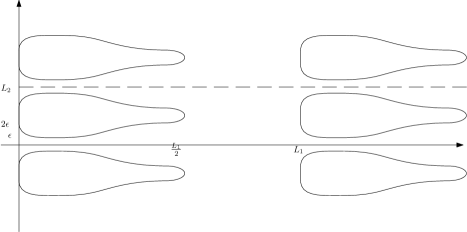
Figure 3: The periodic domain $\Omega_{3}$

The idea is to choose this domain in such a way that the narrow passages open in an abrupt way to the left, so that propagation will be blocked in this direction, but gently to the right, so that the solution will be able to pass, as in the case of the periodic cylinder of Section 6.1.

We shall build a function $h\in C([0,\frac{L_{1}}{2}])\cap C^{\infty}((0,\frac{L_{1}}{2}))$ to parametrize the boundary of $K$. More specifically, we define $K\subset[0,L_{1})\times[0,L_{2})$ by

$$K\cap(\{0\}\times\mathbb{R})=\{0\}\times[2\varepsilon,L_{2}-2\varepsilon],$$

and

$$\partial K\cap\left(\left(0,\frac{L_{1}}{2}\right]\times\left[0,\frac{L_{2}}{2}\right]\right)=\left\{(s,h(s))\ :\ s\in\left[0,\frac{L_{1}}{2}\right]\right\},$$

then reflected by symmetry with respect to the line $\{x\cdot e_{2}=L_{2}/2\}$:

$$\partial K\cap\left(\left(0,\frac{L_{1}}{2}\right]\times\left[\frac{L_{2}}{2},L_{2}\right]\right)=\left\{(s,L_{2}-h(s))\ :\ s\in\left[0,\frac{L_{1}}{2}\right]\right\}.$$

For $\Omega_{3}$ to be smooth, we need $h^{(n)}(0^{+})=-\infty$ and $h^{(n)}(\frac{L_{1}}{2}^{-})=+\infty$, for any $n\geq 1$.

Let $\varepsilon\in(0,1)$, $\kappa>0$, to be chosen later. We define $h$ as follows: first, on $[0,\frac{3}{\varepsilon^{2}}]$, we set

$$\begin{cases}h(0)=2\varepsilon,\\ h^{\prime}(s)\leq 0,\quad&s\in(0,1],\\ h(s)=\varepsilon,\quad&s\in[1,\varepsilon^{-2}],\\ 0\leq h^{\prime}(s)\leq\varepsilon^{2},\quad&s\in[\varepsilon^{-2},2\varepsilon^{-2}],\\ h(s)=1,\quad&s\in[2\varepsilon^{-2},3\varepsilon^{-2}].\end{cases}$$ (6.42)

Now, to define $h$ on $[\frac{3}{\varepsilon^{2}},\frac{L_{1}}{2}]$, we introduce the following cut-off function $\chi\in C^{\infty}([0,1))$ such that

$$\begin{cases}\chi^{(n)}(0)=0,\quad&n\geq 0,\\ \chi^{\prime}(s)\geq 0,\quad&s\in[0,1),\\ \chi(1^{-})=1,\ \chi^{(n)}(1^{-})=+\infty,\quad&n\geq 1,\end{cases}$$ (6.43)

and we set

$$h(s)=1+\kappa\chi\left(\frac{1}{\kappa}\left(s-\frac{3}{\varepsilon^{2}}\right)\right)\quad\text{ for }\ s\in\left[\frac{3}{\varepsilon^{2}},\frac{3}{\varepsilon^{2}}+\kappa\right].$$

Finally, we define

$$L_{1}:=2\left(\frac{3}{\varepsilon^{2}}+\kappa\right)\ \text{ and }~\ L_{2}:=2(1+\kappa).$$

The graph of the function $h$ is depicted in Figure 4.

Figure 4: Graph of the function $h$

We have defined the domain $\Omega_{3}$, depending on $\varepsilon,\kappa$. Let us see how we choose these parameters. To start with, we take $R>0$ large enough so that there is a positive solution $u_{R}$ of (5.31). Thanks to (5.32) we can choose $R>1$ in such a way that

$$M:=\min_{x\in\overline{B}_{1}}u_{R}(x)\in(\theta,1).$$ (6.44)

Next, we take $\kappa$ large enough and $\varepsilon$ small enough so that $\Omega_{3}$ satisfies the following exterior ball condition at every $x\in(\partial\Omega)\cap([\frac{2}{\varepsilon^{2}},\frac{L_{1}}{2}]\times\mathbb{R})$:

$$\exists y\in\Omega_{3}^{c}\ \text{ such that }\ \overline{B}_{R^{2}}(y)\cap\overline{\Omega}_{3}=\{x\}.$$ (6.45)

(Observe that $\kappa$ acts as a sialation in the definition of $h$.) Now, Proposition 6.2 applied to the periodic cylinder

$$\tilde{\Omega}_{3}:=\Omega_{3}\cap(\mathbb{R}\times(0,L_{2}))$$

and $b=-1$, yields that, if the measure of $\tilde{\Omega}_{3}\cap\big{(}(0,1)\times\mathbb{R}\big{)}$ is small enough, then problem (6.38) admits a solution in the truncated cylinder ${\Omega}_{3}\cap\big{(}(-\infty,1)\times(0,L_{2})\big{)}$. Since this measure is smaller than $4\varepsilon$, up to decreasing $\varepsilon$ we assume that this condition is fulfilled. We further increase $\kappa$ and decrease $\varepsilon$ so that

$$\kappa\geq 4R\quad\text{and}\quad R\leq\frac{1}{2\varepsilon}.$$ (6.46)

6.2.2 Invasion towards right

In this subsection, the domain $\Omega_{3}$ and the constant $R>1$ are the ones constructed before, and $u_{R}$ is the solution to (5.31) extended by $0$ outside $\overline{B}_{R}$. We recall that it is radially symmetric and decreasing and satisfies (6.44). We let $\mathcal{C}$ denote the following periodicity cell:

$$\mathcal{C}:=[2R,L_{1}+2R]\times\left[-\frac{L_{2}}{2},\frac{L_{2}}{2}\right].$$

Here is the key result to prove statement $(i)$ of Theorem 1.10.

Proposition 6.3.

Let $u$ be the solution of (1.11) emerging from the initial datum $u_{R}(\cdot-2Re_{1})$. Then, there is $T>0$ such that, for any $n\in\mathbb{N}$, there holds

$$u(t,x)>M>\theta\quad\text{ for }\ t\geq(n+1)T,\ x\in\overline{\Omega}_{3}\cap\bigcup_{\begin{subarray}{c}a\in\mathbb{N}\cup\{0\},\ b\in\mathbb{Z}\\ a+|b|\leq n\end{subarray}}\left(\mathcal{C}+\{aL_{1}e_{1}+bL_{2}e_{2}\}\right).$$

The proof of this proposition is achieved through a series of intermediate lemmas. The first two concern some geometric properties of $\Omega_{3}$.

Lemma 6.4.

Let $\lambda\in[2R,3\varepsilon^{-2}-R]\cup[L_{1}-R,L_{1}]$. Then property (6.37) holds with $z=\lambda e_{1}$, and therefore $u_{R}(\cdot-\lambda e_{1})$ is a generalized subsolution to (1.11).

Proof.

Observe preliminarily that $2R<3\varepsilon^{-2}-R$ because $R<\varepsilon^{-1}<\varepsilon^{-2}$ by (6.46). We have already seen at the beginning of Section 6 that property (6.37) is equivalent to have that $u_{R}(\cdot-z)$ (restricted to $\overline{\Omega}_{3}$) is a generalized subsolution of (1.11).

Take $\lambda\in[2R,3\varepsilon^{-2}-R]$ and $x\in(\partial\Omega_{3})\cap\overline{B}_{R}(\lambda e_{1})$. Then $1<R\leq x\cdot e_{1}\leq 3\varepsilon^{-2}$ and $x\cdot e_{2}=\pm h(x\cdot e_{1})$. By symmetry, we can restrict to the case $x\cdot e_{2}=h(x\cdot e_{1})$. For such values of $x$ we have that $h^{\prime}(x\cdot e_{1})\leq\varepsilon^{2}$. Because the unit exterior normal at the point $x\in\partial\Omega_{3}$, $\nu(x)$, is positively collinear to $(-h^{\prime}(x\cdot e_{1}),1)$, there holds

$$\begin{array}[]{ll}\big{|}(-h^{\prime}(x\cdot e_{1}),1)\big{|}(\lambda e_{1}-x)\cdot\nu(x)&=-h^{\prime}(x\cdot e_{1})(\lambda-x\cdot e_{1})-h(x\cdot e_{1})\\ &\leq\varepsilon^{2}|x\cdot e_{1}-\lambda|-\varepsilon\\ &\leq\varepsilon^{2}R-\varepsilon\\ &\leq 0,\end{array}$$

where the last inequality comes from (6.46).

Let us check property (6.37) with $z=\lambda e_{1}$ and $\lambda\in[L_{1}-R,L_{1}]$. Thanks to the periodicity of $\Omega_{3}$, we reduce to the case $\lambda\in[-R,0]$. Take $x\in(\partial\Omega_{3})\cap\overline{B}_{R}(\lambda e_{1})$. Hence $x\cdot e_{1}\in[-2R,R]$ and thus in particular $x\cdot e_{1}>-\frac{L_{1}}{2}$ thanks to (6.46). It follows that $x\cdot e_{1}\geq 0$, whence $x\cdot e_{1}\geq\lambda$. Hence, by the same computation as above, using the fact that $h$ is decreasing on $[0,R]$ we derive (6.37). ∎

Lemma 6.5.

Let $z\in\Omega_{3}$ be such that $z\cdot e_{1}\in[3\varepsilon^{-2}-R,L_{1}-2R]$ and $d(z,\partial\Omega_{3})\geq 1$, where $d(z,\partial\Omega_{3})$ denotes the distance between $z$ and $\partial\Omega_{3}$. Then property (6.37) holds and therefore $u_{R}(\cdot-z)$ is a generalized subsolution to (1.11).

Proof.

Take $z$ as in the statement of the lemma. Assume that there exists $x\in(\partial\Omega_{3})\cap\overline{B}_{R}(z)$. We have that $L_{1}>x\cdot e_{1}\geq 3\varepsilon^{-2}-2R\geq 2\varepsilon^{-2}$ by (6.46) and therefore property (6.45) holds. We see that $|x-y|=R^{2}$, $|x-z|<R$ and $|z-y|\geq R^{2}+1$. From this we get

$$\begin{split}(z-x)\cdot\nu(x)&=\frac{(z-x)\cdot(y-x)}{|y-x|}\\ &=\frac{|z-x|^{2}+|y-x|^{2}-|z-y|^{2}}{2|y-x|}\\ &\leq\frac{R^{2}+R^{4}-(R^{2}+1)^{2}}{2R^{2}}\\ &<0,\end{split}$$

whence property (6.37). ∎

Now, for the sake of clarity, we state a lemma that gathers the previous two under a more useful form.

Lemma 6.6.

The set $\mathcal{S}$ defined by

$$\begin{split}\mathcal{S}:=&([2R,L_{1}]\times\{0\})\\ &\cup\{z~\in\Omega_{3}\cap\mathcal{C}\ :\ z\cdot e_{1}\in[3\varepsilon^{-2}-R,L_{1}-2R]\ \text{ and }\ d(z,\partial\Omega_{3})\geq 1\}\\ &\cup\{z\in(\overline{\Omega}_{3}\setminus B_{3R}(L_{1}e_{1}))\cap\mathcal{C}~\ :\ z\cdot e_{1}\in[L_{1}-2R,L_{1}]\}\end{split}$$

satisfies the following properties:

1. The set $\mathcal{S}$ is a path-connected subset of $\Omega_{3}$.

2. For $z\in\mathcal{S}$, $u_{R}(\cdot-z)$ is a generalized stationary subsolution of (1.11).

The set $\mathcal{S}$, depicted in Figure 5, is a “slidable” region in $\Omega_{3}\cap\mathcal{C}$ for the centers of the subsolutions $u_{R}(\cdot-z)$. Property $(ii)$ follows from Lemmas 6.4-6.5, except when $z$ belongs to the third set in the definition of $\mathcal{S}$. But in such case condition (6.37) is readily derived by noticing that, thanks to (6.46), the set $(\partial\Omega)\cap\overline{B}_{R}(z)$ is contained in the vertical line $\{x\cdot e_{1}=L_{1}\}$.

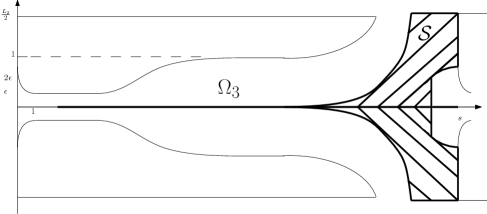
Figure 5: The “slidable” region $\mathcal{S}$

The last auxiliary result, which will allow us to “jump” to the right of the narrow passage, concerns the solution of the following Cauchy problem in $B_{R^{\prime}}$, with $R^{\prime}>R$:

$$\left\{\begin{array}[]{rll}\partial_{t}v-\Delta v&=f(v),&t>0,\ x\in B_{R^{\prime}}\\ v&=0,&t>0,\ x\in\partial B_{R^{\prime}}\\ v(0,x)&=u_{R}(x),&x\in B_{R^{\prime}}.\end{array}\right.$$ (6.47)

Lemma 6.7.

Let $v_{R^{\prime}}$ be the solution of (6.47) with $R^{\prime}>R$. Then, for any $t>0$, the function $v_{R^{\prime}}(t,\cdot)$ is radially symmetric and decreasing. Moreover, it satisfies

$$\forall x\in B_{R^{\prime}-R},\quad\lim_{t\to+\infty}v_{R^{\prime}}(t,x)>M^{\prime}:=u_{R}(0).$$

Proof.

The symmetry property is immediately inherited from the initial datum $u_{R}$ due to the uniqueness of solutions for the parabolic problem (6.47). We show that the same is true for the radial monotonicity using a standard moving plane technique. Let $H$ be a straight line in $\mathbb{R}^{2}$ intersecting $B_{R^{\prime}}(0)$ which does not contain the origin and let $\Sigma$ denote the orthogonal symmetry with respect to $H$. We define

$$w_{R^{\prime}}(t,x):=v_{R^{\prime}}(t,\Sigma(x)),\quad\text{ for }\ t~>0,\ x\in\Sigma(B_{R^{\prime}}).$$

Then, $w_{R^{\prime}}$ is a solution of (6.47) set on $\Sigma(B_{R^{\prime}})$ arising from the initial datum $u_{R^{\prime}}(\Sigma(\cdot))$. Now, consider the domain $U$ given by the intersection between $\Sigma(B_{R^{\prime}})$ and the half-plane bounded by $H$ and containing the origin. Observe that $U\subset B_{R^{\prime}}$. On the one hand, $u_{R^{\prime}}$ and $v_{R^{\prime}}$ coincide on $H\cap\overline{B}_{R^{\prime}}$ for all $t$, because $\Sigma$ is the identity there. On the other hand, $u_{R^{\prime}}>v_{R^{\prime}}=0$ on $\partial U\setminus H$. Moreover, for $x\in U$ there holds $d(x,0)<d(x,\Sigma(0))$. Because $u_{R}$ is radially decreasing, it follows that $u_{R^{\prime}}\geq u_{R^{\prime}}(\Sigma(\cdot))$ in $U$. The parabolic comparison principle then yields $v_{R^{\prime}}(t,x)\geq w_{R^{\prime}}(t,x)$ for all $t>0$, $x\in U$. This being true for every line $H$, we deduce that $v_{R^{\prime}}(t,\cdot)$ is radially decreasing.

We derive the last statement of the lemma using the sliding method. Because the initial datum $u_{R}$ is a generalized stationary subsolution for the parabolic problem (6.47), we have that $v_{R^{\prime}}(t,x)$ is increasing with respect to $t$ and converges to a stationary solution $v_{\infty}>u_{R}$ of (6.47) as $t$ goes to $+\infty$. Fix a direction $e\in S^{N-1}$. For $s\in[0,R^{\prime}-R)$, define $u^{s}_{R}:=u_{R}(\cdot-se)$. We claim that $u^{s}_{R}<v_{\infty}$ in $B_{R}^{\prime}$ for all $s\in[0,R^{\prime}-R)$. Assume by contradiction that this is not the case, then call $s^{\star}$ the infimum of the $s\in[0,R^{\prime}-R)$ for which $u^{s}_{R}<v_{\infty}$ fails. We deduce that there is a contact point between $v_{\infty}$ and $u_{R}^{s^{\star}}$, i.e., $\min_{B_{R^{\prime}}}(v_{\infty}-u_{R}^{s^{\star}})=0$. The elliptic strong maximum principle then yields $v_{\infty}\equiv u_{R}^{s^{\star}}$, which is impossible because $u_{R}^{s^{\star}}$ is compactly supported in $B_{R^{\prime}}$. This proves the claim. We infer in particular that $v_{\infty}>M^{\prime}:=u_{R}(0)$ in the segment connecting $0$ (included) to $(R^{\prime}-R)e$ (excluded). The desired property then follows from the arbitrariness of $e\in S^{N-1}$. ∎

These lemmas at hand, we can turn to the proof of Proposition 6.3.

Proof of Proposition 6.3..

The proof is divided into three steps. Let $u$ denote the solution of (1.11) set on the domain $\Omega_{3}$ given by (6.41) emerging from the initial datum $u_{R}(\cdot-2Re_{1})$. Because $2Re_{1}$ belongs to the set $\mathcal{S}$ of Lemma 6.6, this initial datum is a generalized subsolution to (1.11). As a consequence, $u(t,x)$ is increasing with respect to $t$ and that it converges as $t\to+\infty$ locally uniformly in $x\in\overline{\Omega}_{3}$ to a stationary solution of (1.11), that we call $u_{\infty}$. We claim that $u_{\infty}$ fulfills the following properties:

$$u_{\infty}>M\quad\text{ in }\ \overline{\Omega}_{3}\cap\mathcal{C},$$ (6.48)

$$\forall z\in\{0,L_{1}e_{1},L_{2}e_{2},-L_{2}e_{2}\},\quad u_{\infty}(\cdot+z)>u_{R}(\cdot-2Re_{1}).$$ (6.49)

Step 1. Estimate in the “slidable” region $\mathcal{S}$.
We start with showing that

$$u_{\infty}>M\quad\text{ in }\ (\mathcal{S}+\overline{B}_{1})\cap\overline{\Omega}_{3},$$ (6.50)

where $M$ is given in (6.44). Consider an arbitrary $z$ in the set $\mathcal{S}$ defined in Lemma 6.6. Because $\mathcal{S}$ is path-connected, there exists a continuous path $\gamma:[0,1]\to\mathcal{S}$ such that $\gamma(0)=2Re_{1}$, $\gamma(1)=z$. Let $(u^{s}_{R})_{s\in[0,1]}$ be the continuous family of functions defined by

$$u^{s}_{R}:=u_{R}(\cdot-\gamma(s)).$$

We know from Lemma 6.6 that all these functions are generalized subsolutions to (1.11). Furthermore, $u^{0}_{R}$ coincides with the initial datum of $u$, whence $u^{0}_{R}<u_{\infty}$. Then, the same sliding method as in the proof of Lemma 6.7 shows that $u^{s}_{R}<u_{\infty}$ for all $s\in[0,1]$, and thus in particular

$$\forall z\in\mathcal{S},\quad u_{\infty}>u_{R}(\cdot-z).$$ (6.51)

We eventually deduce from (6.44) that $\min_{\overline{B}_{1}(z)}u_{\infty}>\min_{\overline{B}_{1}}u_{R}=M$. Because $z\in\mathcal{S}$ was arbitrary, (6.50) follows.

Step 2. “Jumping above” the narrow passage.
In this step, we show that

$$u_{\infty}>M^{\prime}\quad\text{ in }\ \Omega_{3}\cap B_{3R}(L_{1}e_{1}),$$ (6.52)

where $M^{\prime}$ is given by Lemma 6.7. By (6.51) we know that $u_{\infty}>u_{R}(\cdot-L_{1}e_{1})$. Consider the function $v_{4R}$ provided by Lemma 6.7 with $R^{\prime}=4R$. We extend it by $0$ outside $B_{4R}$ and consider its restriction to $\Omega_{3}$. Let us show that $v_{4R}$ is a generalized subsolution for (1.11). This property is trivial for the first equation. For the second one, being $v_{4R}(t,\cdot)$ radially symmetric and decreasing thanks to Lemma 6.7, we know that we need to check that condition (6.37) holds with $z=0$ and $R$ replaced by $4R$. This is readily achieved by noticing that $(\overline{B}_{4R}\cap\partial\Omega)\subset([0,4R]\times[-\frac{L_{2}}{2},\frac{L_{2}}{2}])$ thanks to (6.46), and then using the fact that $h$ is non-increasing on $[0,4R]$. By periodicity, the function $v_{4R}(\cdot,\cdot-L_{1}e_{1})$ is a subsolution to (1.11) too. In addition, it is equal to $u_{R}(\cdot-L_{1}e_{1})<u_{\infty}$ at time $t=0$. It then follows from the comparison principle that $u_{\infty}>v_{4R}(t,\cdot-L_{1}e_{1})$ for all $t>0$. Property (6.52) eventually follows from the last statement of Lemma 6.7.

Step 3. Conclusion
Gathering together (6.50) and (6.52) we obtain (6.48). Next, observe that the set

$$\mathcal{S}\cup(\mathcal{S}+\{L_{2}e_{2}\})\cup(\mathcal{S}-\{L_{2}e_{2}\})$$

is path-connected and contains the points

$$2Re_{1},\qquad 2Re_{1}+L_{2}e_{2},\qquad 2Re_{1}-L_{2}e_{2}.$$

We can then argue as in the step 1 to derive (6.51) at those points $z$. The same conclusion holds with $z=2Re_{1}+L_{1}e_{1}$ by (6.52). This proves (6.49).

Now, because the convergence of $u(t,x)$ to $u_{\infty}$ is locally uniform in $x\in\overline{\Omega}_{3}$ as $t$ goes to $+\infty$, properties (6.48)-(6.49) hold true with $u_{\infty}$ replaced by $u(t,\cdot)$ for every $t$ larger than some $T$. Owing to the comparison principle, it follows from the latter that

$$\forall a\in\{0,1\},\ b\in\{-1,0,1\}\ \text{ such that }\ a+|b|\leq 1,\quad u(\cdot+T,\cdot+aL_{1}e_{1}+bL_{2}e_{2})>u.$$

Then, by iteration, for all $n\in\mathbb{N}$ there holds

$$\forall a\in\mathbb{N}\cup\{0\},\ b\in\mathbb{Z}\ \text{ such that }\ a+|b|\leq n,\quad u(\cdot+nT,\cdot+aL_{1}e_{1}+bL_{2}e_{2})>u.$$

The proof is thereby achieved because $u(t,x)>M$ for $t\geq T$, $x\in\overline{\Omega}_{3}\cap\mathcal{C}$. ∎

6.2.3 Proof of Theorem 1.10

We first show the invasion property in the direction $e_{1}$, and then the blocking in the direction $-e_{1}$.

Proof of Theorem 1.10..

Let $\Omega_{3}$, $R$, $L_{1}$ and $L_{2}$ be as in the previous subsections.

Statement $(i)$.
Consider the solution $u$ of Proposition 6.3. Let us show that Theorem 1.10$(i)$ holds for $u$. First, because $u_{R}<1$, the parabolic comparison principle yields $u\leq 1$. Now, call $c:=L_{1}/T$, with $T$ given by Proposition 6.3. Take $c_{1},c_{2}$ such that $0<c_{1}<c_{2}<c$. Consider a diverging sequence $(t_{n})_{n\in\mathbb{N}}$ and a sequence $(x_{n})_{n\in\mathbb{N}}$ in $\Omega_{3}$ such that

$$\forall n\in\mathbb{N},\quad c_{1}t_{n}\leq x_{n}\cdot e_{1}\leq c_{2}t_{n},\qquad(x_{n}\cdot e_{2})_{n\in\mathbb{N}}\text{ is bounded}.$$

Consider then the sequence $(k_{n})_{n\in\mathbb{N}}$ in $\mathbb{Z}$ for which $0\leq x_{n}\cdot e_{1}-k_{n}L_{1}<L_{1}$. This sequence diverges to $+\infty$ because $(x_{n}\cdot e_{1})_{n\in\mathbb{N}}$ does. We define the translated functions

$$u^{n}:=u(\cdot+t_{n},\cdot+k_{n}e_{1}L_{1}).$$

The sequence $(u^{n})_{n\in\mathbb{N}}$ converges as $n$ goes to $+\infty$ (up to extraction) locally uniformly in $t\in\mathbb{R}$, $x\in\overline{\Omega}_{3}$, to a function $u^{\infty}$ which is an entire solution of (1.11). We claim that

$$\forall t\in\mathbb{R},\ \forall x\in\Omega_{3},\quad u^{\infty}(t,x)\geq M,$$ (6.53)

where $M$ is given by (6.44). Fix $t\in\mathbb{R}$ and $x\in\Omega_{3}$. Set $m_{n}:=\left\lfloor{\frac{t+t_{n}}{T}}\right\rfloor$-1, where $\lfloor\cdot\rfloor$ stands for the integer part. We compute

$$k_{n}\leq\frac{x_{n}\cdot e_{1}}{L_{1}}\leq\frac{c_{2}}{L_{1}}t_{n}<\frac{c_{2}}{L_{1}}(m_{n}+2)T-\frac{c_{2}}{L_{1}}t=(m_{n}+2)\frac{c_{2}}{c}-\frac{c_{2}}{L_{1}}t.$$

Because $c_{2}<c$, we find that $m_{n}-k_{n}\to+\infty$ as $n$ goes to $+\infty$. Consequently, for $n$ large enough, there holds

$$t+t_{n}\geq(m_{n}+1)T\ \text{ and }\ x+k_{n}L_{1}e_{1}\in\bigcup_{\begin{subarray}{c}a\in\mathbb{N}\cup\{0\},\ b\in\mathbb{Z}\\ a+|b|\leq m_{n}\end{subarray}}\left(\mathcal{C}+\{aL_{1}e_{1}+bL_{2}e_{2}\}\right),$$

and therefore $u^{n}(t,x)>M$ thanks to Proposition 6.3. This proves (6.53). Recall that $M>\theta$. Then Lemma 3.1 yields $u^{\infty}\equiv 1$. This means that property $(i)$ of Theorem 1.10 holds for the solution $u$. As usual, one then extend the result to the class of initial data stated in the theorem by arguing as in the proof of Theorem 1.2.

Statement $(ii)$. 
We shall make use of the blocking property for cylinders. Consider the cylinder

$$\tilde{\Omega}_{3}:=\Omega_{3}\cap(\mathbb{R}\times(0,L_{2})).$$

Because of the choice of $\varepsilon$ in the construction of $\Omega_{3}$, we can apply Proposition 6.2 to this cylinder with $b=-1$ and get a positive solution $w$ to (6.38). We first extend $w$ to the whole $\tilde{\Omega}_{3}$ by setting $w(x)=1$ for $x\cdot e_{1}\geq 1$. Next, we extend it by periodicity in the direction $e_{2}$, with period $L_{2}$. Because $\nabla w(x)\cdot e_{2}=0$ for $x\cdot e_{2}\in L_{2}\mathbb{Z}$, we have that $w$ is a generalized supersolution to (1.11). Consider now a compactly supported initial datum $u_{0}\leq 1$. We can find $k\in\mathbb{Z}$ such that $u_{0}\leq w(\cdot+kL_{1}e_{1})$. The parabolic comparison principle then yields $u(t,x)\leq w(x+2L_{1}ke_{1})$, for all $t>0,\ x\in\Omega_{3}$. Statement $(ii)$ eventually follows from the last property of (6.38). ∎

References

- [1] D. G. Aronson and H. F. Weinberger. Multidimensional nonlinear diffusion arising in population genetics. Adv. in Math., 30(1):33–76, 1978.
- [2] H. Berestycki, J. Bouhours, and G. Chapuisat. Front blocking and propagation in cylinders with varying cross section. Calc. Var. Partial Differential Equations, 55(3):Paper No. 44, 32, 2016.
- [3] H. Berestycki and F. Hamel. Front propagation in periodic excitable media. Comm. Pure Appl. Math., 55(8):949–1032, 2002.
- [4] H. Berestycki and F. Hamel. Non-existence of travelling front solutions of some bistable reaction-diffusion equations. Adv. Differential Equations, 5(4-6):723–746, 2000.
- [5] H. Berestycki, F. Hamel, and H. Matano. Bistable traveling waves around an obstacle. Comm. Pure Appl. Math., 62(6):729–788, 2009.
- [6] H. Berestycki, F. Hamel, and N. Nadirashvili. The speed of propagation for KPP type problems. I. Periodic framework. J. Eur. Math. Soc. (JEMS), 7(2):173–213, 2005.
- [7] H. Berestycki, F. Hamel, and L. Rossi. Liouville-type results for semilinear elliptic equations in unbounded domains. Ann. Mat. Pura Appl. (4), 186(3):469–507, 2007.
- [8] H. Berestycki and P.-L. Lions. Une méthode locale pour l’existence de solutions positives de problèmes semi-linéaires elliptiques dans . J. Analyse Math., 38:144–187, 1980.
- [9] A.-P. Calderón. Lebesgue spaces of differentiable functions and distributions. In Proc. Sympos. Pure Math., Vol. IV, pages 33–49. American Mathematical Society, Providence, R.I., 1961.
- [10] R. Ducasse. Propagation properties of reaction-diffusion equations in periodic domains. Preprint, 2017.
- [11] A. Ducrot. A multi-dimensional bistable nonlinear diffusion equation in a periodic medium. Math. Ann., 366(1-2):783–818, 2016.
- [12] M. I. El Smaily. Min-max formulae for the speeds of pulsating travelling fronts in periodic excitable media. Ann. Mat. Pura Appl. (4), 189(1):47–66, 2010.
- [13] R. A. Fisher. The wave of advantage of advantageous genes. Ann. Eugenics, 7:355–369, 1937.
- [14] Freidlin, M. I. On wavefront propagation in periodic media. in Stochastic analysis and applications, Adv. Probab. Related Topics, vol. 7, pp. 147–166, Dekker, New York, 1984.
- [15] J. Gärtner and M. I. Freĭdlin. The propagation of concentration waves in periodic and random media. Dokl. Akad. Nauk SSSR, 249(3):521–525, 1979.
- [16] B. Gidas, W. M. Ni, and L. Nirenberg. Symmetry and related properties via the maximum principle. Comm. Math. Phys., 68(3):209–243, 1979.
- [17] D. Gilbarg and N. S. Trudinger. Elliptic partial differential equations of second order, volume 224 of Grundlehren der Mathematischen Wissenschaften [Fundamental Principles of Mathematical Sciences]. Springer-Verlag, Berlin, second edition, 1983.
- [18] T. Giletti and L. Rossi. Pulsating fronts for multidimensional bistable and multistable equations. Preprint, 2017.
- [19] A. N. Kolmogorov, I. G. Petrovskiĭ, and N. S. Piskunov. Étude de l’équation de la diffusion avec croissance de la quantité de matière et son application à un problème biologique. Bull. Univ. Etat. Moscow Ser. Internat. Math. Mec. Sect. A, 1:1–26, 1937.
- [20] O. A. Ladyzenskaja, V. A. Solonnikov, and N. N. Ural’ceva. Linear and quasilinear equations of parabolic type. Translated from the Russian by S. Smith. Translations of Mathematical Monographs, Vol. 23. American Mathematical Society, Providence, R.I., 1967.
- [21] G. M. Lieberman. Second order parabolic differential equations. World Scientific Publishing Co. Inc., River Edge, NJ, 1996.
- [22] A. P. Morse. The behavior of a function on its critical set. Ann. of Math. (2), 40(1):62–70, 1939.
- [23] L. Rossi. The Freidlin-Gärtner formula for general reaction terms. Adv. Math., 317:267–298, 2017.
- [24] N. Shigesada, K. Kawasaki, and E. Teramoto. Traveling periodic waves in heterogeneous environments. Theoret. Population Biol., 30(1):143–160, 1986.
- [25] G. Stampacchia. Problemi al contorno ellitici, con dati discontinui, dotati di soluzionie hölderiane. Ann. Mat. Pura Appl. (4), 51:1–37, 1960.
- [26] E. M. Stein. Singular integrals and differentiability properties of functions. Princeton Mathematical Series, No. 30. Princeton University Press, Princeton, N.J., 1970.
- [27] H. F. Weinberger. On spreading speeds and traveling waves for growth and migration models in a periodic habitat. J. Math. Biol., 45(6):511–548, 2002.
- [28] J. X. Xin. Existence and nonexistence of traveling waves and reaction-diffusion front propagation in periodic media. J. Statist. Phys., 73(5-6):893–926, 1993.
- [29] X. Xin. Existence and stability of traveling waves in periodic media governed by a bistable nonlinearity. J. Dynam. Differential Equations, 3(4):541–573, 1991.
- [30] X. Xin. Existence and uniqueness of travelling waves in a reaction-diffusion equation with combustion nonlinearity. Indiana Univ. Math. J., 40(3):985–1008, 1991.
- [31] A. Zlatos. Existence and non-existence of transition fronts for bistable and ignition reactions. Preprint, 2015.