Production of $\chi_{c}$ pairs in $k_{T}$-factorization

Abstract

We calculate the production of pairs of $\chi_{c}(J)$ mesons with all possible combinations of $J=0,1,2$. The leading order production mechanism is the crossed-channel gluon exchange in the gluon-gluon fusion reaction.

The building blocks are the vertices $g^{*}g^{*}\to\chi_{c}(J)$ for off shell gluons. We stick to the color-singlet model and calculate the gluon fusion vertices in the limit of heavy quarks with nonrelativistic motion in the bound state.

These vertices are used to construct the $g^{*}g^{*}\to\chi_{c}(J_{1})\chi_{c}(J_{2})$ amplitudes. We then calculate hadron-level cross sections using the $k_{T}$-factorization approach. In our numerical predictions, we use the KMR-type unintegrated gluon distributions. Several differential distributions at the $pp$ center of mass energy $\sqrt{s}=8\,{\rm TeV}$ are shown.

The salient feature of the $t$ and $u$-channel gluon exchange are the broad distributions in rapidity difference $\Delta y$ between $\chi_{c}$ mesons.

I Introduction

Recently, cross sections for the production of $J/\psi$-pairs were measured at the Tevatron Abazov:2014qba and the LHC CMS_jpsijpsi ; ATLAS_jpsijpsi ; Aaij:2016bqq ; Aaij:2011yc . There remain a number of puzzles, especially with the CMS and ATLAS data. Here the leading order of ${\cal{O}}(\alpha_{S}^{4})$ (see e.g. JJ_kt ; Baranov:2012re ) is clearly not sufficient. The double parton scattering (DPS) contribution was claimed to be large or even dominant in some corners of the phase space, when the rapidity distance $\Delta y$ between two $J/\psi$ mesons is large. However the effective cross sections $\sigma_{\rm eff}$ found from empirical analyses are about a factor $2.5$ smaller than the usually accepted $\sigma_{\rm eff}=15\,\rm{mb}$. It is an open issue at the moment whether this points to a nonuniversality of $\sigma_{\rm eff}$ or whether there are additional single parton scattering mechanisms which can alleviate the tension.

The production of quarkonium pairs is interesting in a broader context. Here we wish to consider production of pairs of $\chi_{c}$ mesons. This process is more difficult to measure experimentally but interesting from the theoretical point of view. A feed down to the double $J/\psi$ channel is interesting in the context of the puzzles mentioned above.

The single-inclusive $\chi_{c}$ meson production was a topic of both experimental Aaij:2013dja ; Chatrchyan:2012ub ; ATLAS:2014ala and theoretical Hagler:2000dd ; Kniehl:2006sk ; Likhoded:2014kfa ; Baranov:2015yea ; Cisek:2016uxz studies. The cross section for single $\chi_{c}$ production is rather large. The nonrelativistic perturbative QCD is the standard theoretical approach in this context. In leading order the gluon fusion $g^{*}g^{*}\to\chi_{c}(J),J=0,1,2$ is the underlying production mechanism. The $k_{T}$-factorization approach provides a reasonable description of the experimental data Baranov:2015yea ; Cisek:2016uxz .

In the present letter we shall include the production of all combinations of $\chi_{c}$ meson pair production. The cross section will be calculated in $k_{T}$-factorization approach using newly derived off-shell matrix elements for the $g^{*}g^{*}\to\chi_{c}(i)\chi_{c}(j)$ process.

A first evaluation of the total cross section will be given. We also show some differential distributions.

I.1 The $pp\to\chi_{c}(J_{1})\chi_{c}(J_{2})X$ reaction, formalism

It was shown in LS2015 ; LLP2016 that the $\chi_{c}J/\psi$ pair production is possible only at $O(\alpha_{s}^{5})$, while forbidden at $O(\alpha_{s}^{4})$ due to $C$ parity conservation. In contrast, the production of $\chi_{c}(J_{1})\chi_{c}(J_{2})$, see Fig.1, is possible already at the $O(\alpha_{s}^{4})$ order.

Of special importance for us is the fact that $\chi_{c}\chi_{c}$ states are produced by the crossed-channel one-gluon exchange mechanism. This implies that the production amplitudes are flat as a function of $g^{*}g^{*}$ center of mass energy, which implies broad distributions in the rapidity distance $\Delta y$ between the produced $\chi_{c}$-mesons.

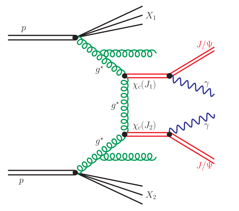
Figure 1: A diagrammatic representation of the leading order mechanisms for $pp\to\chi_{c}(J_{1})\chi_{c}(J_{2})\to(J/\psi+\gamma)(J/\psi+\gamma)$ reaction.

According to our knowledge this contribution was not discussed so far in the literature. There was, however, some calculations for $\chi_{c}\chi_{b}$ production protvino .

We consider the gluon-gluon fusion mechanism shown diagramatically in Fig.1. There are altogether six possible combinations of pair production of $\chi_{c}(0),\chi_{c}(1),\chi_{c}(2)$ quarkonia.

In order to calculate the subprocess amplitudes, we first turn to the $g^{*}g^{*}\to\chi_{c}(J)$ vertices.

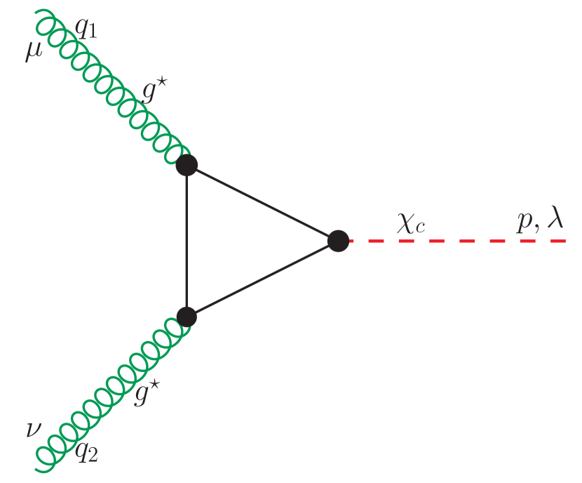
Figure 2: A diagrammatic representation of the $g^{*}g^{*}\to\chi_{c}(\lambda)$ vertex being a building block of corresponding $g^{*}g^{*}\to\chi_{c}(J_{1})\chi_{c}(J_{2})$ and discussed in this section amplitudes.

I.1.1 The $g^{*}g^{*}\to\chi_{c}(J)$ vertices

The $g^{*}g^{*}\to\chi_{c}$ vertices with off-shell gluons (see Fig.2) are building blocks of the elementary $g^{*}g^{*}\to\chi_{c}(J_{1})\chi_{c}(J_{2})$ amplitudes.

Here we follow the general rules of NRQCD as explained e.g. in Guberina:1980dc ; Cho:1995ce ; Cho:1995vh . We restrict ourselves to the color singlet contribution and can write the amplitude for the production of the $\chi_{c}(J)$ meson via the fusion of two gluons as:

$$V^{ab}_{\mu\nu}(J,J_{z};q_{1},q_{2})=4\pi\alpha_{S}{{\rm Tr}[t^{a}t^{b}]\over\sqrt{N_{c}}}\,\sqrt{{2\over M}}\sum_{S_{z},L_{z}}\int{d^{4}k\over(2\pi)^{3}}\delta(k^{0}-{\vec{k}^{2}\over M})\Psi_{1,L_{z}}(\vec{k})$$

$$\times\langle{1,S_{z};1,L_{z}}|{J,J_{z}}\rangle\cdot{\rm{Tr}}[A_{\mu\nu}\Pi_{1,S_{z}}],$$ (1)

following closely the notation of Hagler:2000dd ; Pasechnik:2007hm ; Pasechnik:2009bq ; Pasechnik:2009qc , where these vertices had been calculated for external reggeized gluons. Below we will need the amplitudes (1) for arbitrary off-shell momenta of gluons, not only the multiregge kinematics as in Hagler:2000dd ; Pasechnik:2007hm ; Pasechnik:2009bq ; Pasechnik:2009qc . There is however no additional difficulty related with this. As we concentrate on the color-singlet mechanism, the three-gluon coupling does not enter and we really deal with a QED problem. Consequently the amplitudes (1) fulfill the QED-like gauge invariance conditions:

$$q_{1}^{\mu}V^{ab}_{\mu\nu}(J,J_{z};q_{1},q_{2})=0,q_{2}^{\nu}V^{ab}_{\mu\nu}(J,J_{z};q_{1},q_{2})=0.$$ (2)

The calculation proceeds as follows.

The $g^{*}g^{*}\to Q\bar{Q}$ amplitude is (up to factors)

$$A_{\mu\nu}=\gamma_{\mu}{\hat{p}_{Q}-\hat{q}_{1}+m_{Q}\over(p_{Q}-q_{1})^{2}-m_{Q}^{2}}\gamma_{\nu}+\gamma_{\nu}{\hat{p}_{Q}-\hat{q}_{2}+m_{Q}\over(p_{Q}-q_{2})^{2}-m_{Q}^{2}}\gamma_{\mu}\,.$$ (3)

We parametrize

$$p_{Q}={P\over 2}+k\,,\,p_{\bar{Q}}={P\over 2}-k\,,$$ (4)

In spectroscopic notation, the $\chi_{c}$ mesons are ${}^{2S+1}L_{J}=^{3}P_{J}$ states, where $J=0,1,2$. Therefore the spinorial part of the wavefunction is an $S=1$ spin triplet state, and the relevant projector can be written as

$$\Pi_{S=1,S_{z}} = {1\over 2\sqrt{2}m_{Q}}\,\Big{(}{\hat{P}\over 2}-\hat{k}-m_{Q}\Big{)}\hat{\epsilon}(S_{z})\Big{(}{\hat{P}\over 2}+\hat{k}+m_{Q}\Big{)}.$$ (5)

Now, for the $P$-wave states, we should expand the product $A_{\mu\nu}\hat{\Pi}_{S=1,S_{z}}$ in (1) to the first order in $k$. In fact the Taylor expansion for $P$-waves starts from the term linear in $k$:

$${\rm Tr}[A_{\mu\nu}\Pi_{1,S_{z}}]\rightarrow k_{\alpha}\cdot{\partial\over\partial k_{\alpha}}{\rm Tr}[A_{\mu\nu}\Pi_{1,S_{z}}]\Big{|}_{k=0}\,.$$ (6)

Then, the integration over relative momentum $k$ reduces to the integral

$$\int{d^{3}\vec{k}\over(2\pi)^{3}}k^{\alpha}\Psi_{1,L_{z}}(\vec{k})=-i\sqrt{3\over 4\pi}\,R^{\prime}(0)\cdot\epsilon^{\alpha}(L_{z})\,.$$ (7)

Here $R^{\prime}(0)$ is the derivative of the radial wavefunction at the (spatial) origin.

For convenience, we introduce

$$T_{\mu\nu}(q_{1},q_{2};J,J_{z})\equiv{\sqrt{2}M\over 8}\,\sum_{S_{z},L_{z}}\langle{1,S_{z};1,L_{z}}|{J,J_{z}}\rangle\epsilon_{\alpha}(L_{z})\cdot{\partial\over\partial k_{\alpha}}{\rm Tr}[A_{\mu\nu}\Pi_{1,S_{z}}]\Big{|}_{k=0},$$ (8)

so that our gluon-gluon fusion vertices take the form

$$V^{ab}_{\mu\nu}(J,J_{z};q_{1},q_{2})=-i\,4\pi\alpha_{S}\,\delta^{ab}\,{2R^{\prime}(0)\over\sqrt{\pi N_{c}M^{3}}}\,\sqrt{3}\cdot T_{\mu\nu}(J,J_{z};q_{1},q_{2})\,,$$ (9)

Performing the relevant Dirac-traces, we obtain the explicit expressions for $T_{\mu\nu}(J,J_{z};q_{1},q_{2})$:

1. scalar, $J=0$:

   $$T_{\mu\nu}(0,0;q_{1},q_{2}) = {1\over\sqrt{3}}\,{M^{2}\over(2q_{1}\cdot q_{2})^{2}}\,\Big{\{}g_{\mu\nu}\Big{(}6(q_{1}\cdot q_{2})-q_{1}^{2}-q_{2}^{2}+{(q_{2}^{2}-q_{1}^{2})^{2}\over M^{2}}\Big{)}$$ (10)

   $$+ q_{1\mu}q_{2\nu}\,2\Big{(}{q_{1}^{2}+q_{2}^{2}\over M^{2}}-1\Big{)}\,+q_{2\mu}q_{1\nu}\,2\Big{(}{q_{1}^{2}+q_{2}^{2}\over M^{2}}-3\Big{)}$$

   $$+ q_{1\mu}q_{1\nu}{4q_{2}^{2}\over M^{2}}+q_{2\mu}q_{2\nu}{4q_{1}^{2}\over M^{2}}\Big{\}}$$

2. axial vector, $J=1$:

   $$T_{\mu\nu}(1,J_{z};q_{1},q_{2}) = {i\over\sqrt{2}M}{1\over(q_{1}\cdot q_{2})}\Big{\{}(q_{1}^{2}-q_{2}^{2})\epsilon_{\mu\nu\alpha\beta}(q_{1}+q_{2})^{\alpha}\epsilon^{\beta}(J_{z})$$ (11)

   $$+ {q_{1}^{2}+q_{2}^{2}\over(q_{1}\cdot q_{2})}(a_{\mu}q_{1\nu}-a_{\nu}q_{2\mu})+2(a_{\nu}q_{1\mu}-a_{\mu}q_{2\nu})\Big{\}}\,$$

   with

   $$a_{\mu}=\epsilon_{\mu\rho\alpha\beta}q_{1}^{\rho}q_{2}^{\alpha}\epsilon^{\beta}(J_{z})\,.$$ (12)

3. tensor, $J=2$:

   $$T_{\mu\nu}(2,J_{z};q_{1},q_{2}) = {-M^{2}\over(2q_{1}\cdot q_{2})^{2}}\Big{\{}-g_{\mu\nu}(q_{2}-q_{1})^{\alpha}(q_{2}-q_{1})^{\beta}\epsilon_{\alpha\beta}(J_{z})+4(q_{1}\cdot q_{2})\epsilon_{\mu\nu}(J_{z})$$ (13)

   $$+ 2(q_{2}-q_{1})^{\alpha}\epsilon_{\alpha\nu}(J_{z})q_{2\mu}-2(q_{2}-q_{1})^{\alpha}\epsilon_{\alpha\mu}(J_{z})q_{1\nu}\Big{\}}\,,$$

   where $\epsilon_{\mu\nu}(J_{z})=\sum_{m_{1},m_{2}}\langle{2,J_{z}}|{1,m_{1},1,m_{2}}\rangle\epsilon_{\mu}(m_{1})\epsilon_{\nu}(m_{2})$ is the polarization tensor of the $J=2$ state.

Notice, that

$$2(q_{1}\cdot q_{2})=M^{2}-q_{1}^{2}-q_{2}^{2}\,,$$ (14)

and as gluons are always spacelike $q_{i}^{2}<0$, the denominators of eqs (10 ,11, 13) are always finite.

Besides the QED-like gauge invariance condition, these amplitudes also fulfill the Bose-symmetry

$$T_{\mu\nu}(J,J_{z};q_{1},q_{2})=T_{\nu\mu}(J,J_{z};q_{2},q_{1})\,.$$ (15)

A comment on the $J=1$ axial vector is in order. Here the Landau-Yang theorem forbids the decay of the $\chi_{c}(1)$ into $\gamma\gamma$ or $gg$, and likewise its production through fusion of on-shell photons or gluons. Indeed, in the limit $q_{1}^{2}\to 0,q_{2}^{2}\to 0$, we have

$$T_{\mu\nu}(1,J_{z};q_{1},q_{2})\propto a_{\nu}q_{1\mu}-a_{\mu}q_{2\nu}\,,$$ (16)

which vanishes, when contracted with the polarization vectors of on-shell photons/gluons

$$\epsilon_{1}^{\mu}\epsilon_{2}^{\nu}(a_{\nu}q_{1\mu}-a_{\mu}q_{2\nu})=0,$$ (17)

as required by the Landau-Yang theorem.

I.1.2 The $g^{*}g^{*}\to\chi_{c}(J_{1})\chi_{c}(J_{2})$ amplitudes

Now we wish to discuss the elementary $g^{*}g^{*}\to\chi_{c}(J_{1})\chi_{c}(J_{2})$ amplitudes, which can be obtained from the building blocks discussed above.

In all cases there are two diagrams ($t$ (left) and $u$ (right) in Fig.3).

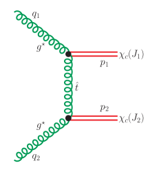
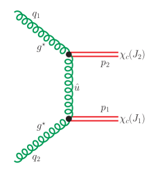
Figure 3: A diagrammatic representation of the generic $g^{*}g^{*}\to\chi_{c}(J_{1})\chi_{c}(J_{2})$ $t$-channel (left) and $u$-channel (right) amplitudes.

We can write the Feynman amplitudes corresponding to these diagrams as

$${\cal M}^{ab}_{\mu\nu}(J_{1},J_{1z},J_{2},J_{2z}) = V^{ac}_{\mu\alpha}(J_{1},J_{1z};q_{1},p_{1}-q_{1}){-g^{\alpha\beta}\delta_{cd}\over\hat{t}}V^{db}_{\beta\nu}(J_{2},J_{2z};p_{2}-q_{2},q_{2})$$ (18)

$$+ V^{ac}_{\mu\alpha}(J_{2},J_{2z};q_{1},p_{2}-q_{1}){-g^{\alpha\beta}\delta_{cd}\over\hat{u}}V^{db}_{\beta\nu}(J_{1},J_{1z};p_{1}-q_{2},q_{1})\,,$$

where $\hat{t}=(p_{1}-q_{1})^{2}=(p_{2}-q_{2})^{2}\,,\,\hat{u}=(p_{2}-q_{1})^{2}=(p_{1}-q_{2})^{2}$. These amplitudes are infrared finite and gauge invariant.

To obtain the $k_{T}$-factorization amplitude one should contract (18) with the polarization vectors of off-shell gluons

$$e_{1\mu}={q_{1T\mu}\over|\vec{q}_{1T}|}\,,\,e_{2\nu}={q_{2T\nu}\over|\vec{q}_{2T}|}\,.$$ (19)

Because of the QED-like Ward identities of the gluon fusion vertices, these polarization vectors are equivalent to the more common Gribov’s polarizations $n^{+}_{\mu},n^{-}_{\nu}$, for incoming gluons in the high-energy kinematics $q_{1\mu}=q_{1}^{+}n^{+}_{\mu}+q_{1T\mu}$, $q_{2\nu}=q_{1}^{+}n^{-}_{\nu}+q_{2T\nu}$.

In the nonrelativistic QCD approach the cross section for $\chi_{c}$ pair production is proportional to $|R^{\prime}(0)|^{4}$. The result is therefore extremely sensitive to the precise value of the wave function derivative at the origin. In our opinion the best estimate of the parameter can be obtained from:

$$\Gamma(\chi_{c}(0^{+})\to\gamma\gamma)={27e_{c}^{4}\alpha_{\rm em}\over m_{c}^{4}}|R^{\prime}(0)|^{2}\;.$$ (20)

From the experimental value of the diphoton decay width PDG one obtains for the $\chi_{c}$ P-wave function squared

$$|R^{\prime}(0)|^{2}=0.042\;{\rm GeV}^{5}.$$ (21)

In the following the $\chi_{c}(J_{1})\chi_{c}(J_{2})$ cross section is calculated within the $k_{T}$-factorization approach including off-shell matrix elements for the $g^{*}g^{*}\to\chi_{c}(J_{1})\chi_{c}(J_{2})$ subprocess and modern unintegrated gluon distributions.

It is well known that about 30 % of prompt single $J/\psi$ production originates from radiative decays $\chi_{c}\to J/\psi+\gamma$ with branching fractions: ${\rm{Br}}(\chi_{c}(0)\to J/\psi\gamma)=1.26\pm 0.06\%$, ${\rm{Br}}(\chi_{c}(1)\to J/\psi\gamma)=33.9\pm 1.2\%$, ${\rm{Br}}(\chi_{c}(2)\to J/\psi\gamma)=19.2\pm 0.7\%$ PDG . Obviously, regarding feed down into the $J/\psi J/\psi$ channel only the $\chi_{c}(1)\chi_{c}(1)$, $\chi_{c}(1)\chi_{c}(2)$ and $\chi_{c}(2)\chi_{c}(2)$ states could give potentially important contributions. The details depend, however, on corresponding matrix elements and cross sections for the $\chi_{c}(J_{1})\chi_{c}(J_{2})$ production.

The cross section for $pp\to\chi_{c}(J_{1})\chi_{c}(J_{2})$ is calculated in the $k_{T}$-factorization approach. The corresponding differential cross section for the production of $\chi_{c}(i)\chi_{c}(j)$ states, where $i$ and $j$ run through $0,1,2$ can be written as:

$$\frac{d\sigma(pp\to\chi_{c}(i)\chi_{c}(j)X)}{dy_{1}dy_{2}d^{2}{\vec{p}}_{1T}d^{2}\vec{p}_{2T}}=\frac{1}{16\pi^{2}(x_{1}x_{2}s)^{2}}{1\over 1+\delta_{ij}}\int\frac{d^{2}\vec{q}_{1T}}{\pi\vec{q}_{1T}^{2}}\frac{d^{2}\vec{q}_{2T}}{\pi\vec{q}_{2T}^{2}}\overline{|{\cal M}_{g^{*}g^{*}\rightarrow\chi_{c}(i)\chi_{c}(j)}^{\rm{off-shell}}|^{2}}$$

$$\times\;\;\delta^{(2)}\left(\vec{q}_{1T}+\vec{q}_{2T}-\vec{p}_{1T}-\vec{p}_{2T}\right){\cal F}(x_{1},\vec{q}_{1T}^{2},\mu_{F}^{2}){\cal F}(x_{2},\vec{q}_{2T}^{2},\mu_{F}^{2})\;.$$ (22)

The unintegrated gluon distribution ${\cal F}(x_{1},\vec{q}_{1T}^{2},\mu_{F}^{2})$ is related to the collinear one through

$$xg(x,\mu_{F}^{2})=\int^{\mu^{2}_{F}}{d\vec{q}^{2}_{T}\over\vec{q}^{2}_{T}}\,{\cal F}(x,\vec{q}_{1T}^{2},\mu_{F}^{2})\,,$$ (23)

and the off-shell matrix element is obtained as

$$\overline{|{\cal M}_{g^{*}g^{*}\rightarrow\chi_{c}\chi_{c}}^{\rm{off-shell}}|^{2}}={1\over(N_{c}^{2}-1)^{2}}\sum_{a,b,J_{1z},J_{2z}}|e_{1\mu}e_{2\nu}{\cal{M}}^{ab}_{\mu\nu}(J_{1},J_{1z},J_{2},J_{2z})|^{2}\;.$$ (24)

The longitudinal momentum fractions $x_{1}$ and $x_{2}$ are calculated from $\chi_{c}$’s transverse masses $m_{Ti}=\sqrt{m_{c}^{2}+\vec{p}_{iT}^{2}}$ and rapidities:

$$x_{1} = {m_{T1}\over\sqrt{s}}e^{y_{1}}+{m_{T2}\over\sqrt{s}}e^{y_{2}}\,,$$

$$x_{2} = {m_{T1}\over\sqrt{s}}e^{-y_{1}}+{m_{T2}\over\sqrt{s}}e^{-y_{2}}\,.$$ (25)

I.2 Results for $\chi_{c}(J_{1})\chi_{c}(J_{2})$ production

We start presentation of our results by showing integrated cross sections. As an example in Table 1 we show cross section in a broad range of $\chi_{c}$ rapidities. We used an unintegrated gluon distribution constructed from the KMR prescription Kimber:2001sc based on the MSTW2008 collinear NLO gluon distribution MSTW08 . For the renormalization scales $\mu^{2}_{r1},\mu^{2}_{r2}$ of the running coupling and factorization scales $\mu^{2}_{F1},\mu^{2}_{F2}$ entering the unintegrated gluon distribution, we choose

$$\mu_{r1}^{2} = \mu^{2}_{F1}={\rm max}\{m_{c}^{2},|\vec{q_{1T}}|^{2}\}\,,$$

$$\mu_{r2}^{2} = \mu^{2}_{F2}={\rm max}\{m_{c}^{2},|\vec{q_{2T}}|^{2}\}\ ,$$ (26)

where these scales refer to the running coupling/gluon distribution coupling to gluon $q_{1}$ or $q_{2}$ respectively. We refrain from a detailed analysis of dependence on the factorization scale, the distributions shown below simply serve to get an impression of the salient features of the production mechanism. A more detailed analysis, including theoretical errors will be given in a future work paperJPsi , where we will address the feeddown into the $J/\psi J/\psi$ channel.

	$\chi_{c}(0)$	$\chi_{c}(1)$	$\chi_{c}(2)$
$\chi_{c}(0)$	1.32	1.71	4.24
$\chi_{c}(1)$	….	0.84	2.88
$\chi_{c}(2)$	….	….	3.45

Table 1: Cross sections in nb for production of different combinations of $\chi_{c}(J_{1})\chi_{c}(J_{2})$ dimeson states for -8 $<y_{1},y_{2}<$ 8 at $\sqrt{s}$ = 8 TeV. The numbers are obtained in the $k_{T}$-factorization approach. We used an unintegrated gluon distribution constructed from the KMR prescription Kimber:2001sc based on the MSTW2008 collinear NLO gluon distribution MSTW08 . In all cases the gauge invariant matrix elements discussed in the present paper were used.

There are six independent cross sections related to the different spin combinations (see Table 1). We see that the cross sections for different spin combinations are of the same order of magnitude.

In Fig.4 we show rapidity distributions for $\chi_{c}$ mesons for different pair combinations. In the left panel we show: $\chi_{c}(0)\chi_{c}(0)$ (solid line), $\chi_{c}(1)\chi_{c}(1)$ (dahed line) and $\chi_{c}(2)\chi_{c}(2)$ (dotted line). In the other panels we show distributions for: $\chi_{c}(0)\chi_{c}(1)$ (solid line), $\chi_{c}(0)\chi_{c}(2)$ (dashed line) and $\chi_{c}(1)\chi_{c}(2)$ (dotted line). In the upper keft panel the distribution of the first listed quarkonium is shown, while the distributions of the second listed quarkonium are shown in the lower panel. Evidently for the nonidentical quarkonia the distribution of the first and second meson are not the same.

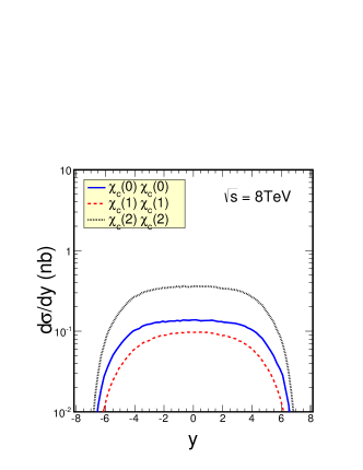
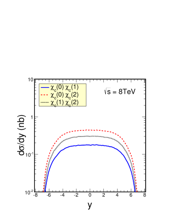
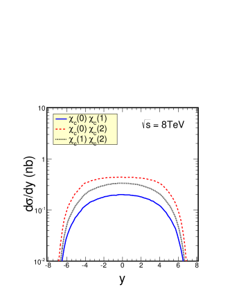
Figure 4: Rapidity distributions of quarkonia for different spin combinations.

In Fig.5 we show similar distributions in quarkonia transverse momenta. The distributions for $\chi_{c}(1)$ quarkonia are less steep than those for the other mesons. This may have important consequences for large transverse momenta, also for $J/\psi$ pair production (CDF, ATLAS, CMS), but goes beyond the scope of the present letter.

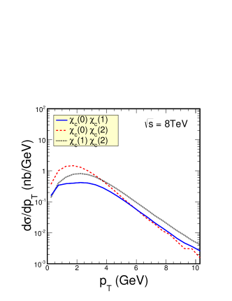
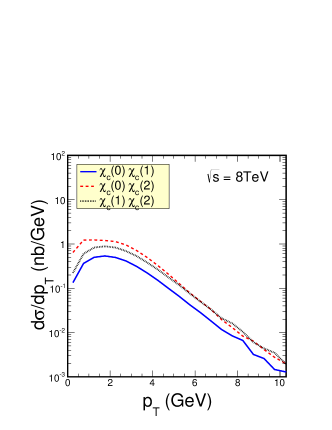
Figure 5: Transverse momentum distributions of quarkonia for different spin combinations.

The exchange of gluons leads to broad distributions in the difference of rapidities $\Delta y$ of the two quarkonia, as shown in Fig.6. All final states have in common also a rather deep dip at $\Delta y=0$. Therefore the $\chi_{c}$ pair production will be potentially important rather for experimental setups that cover a large range in rapidities.

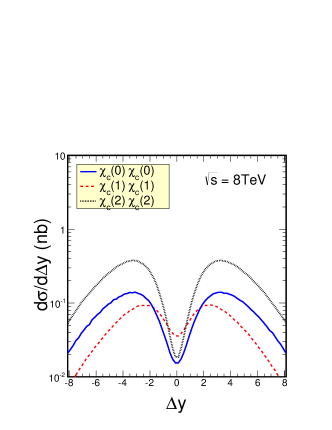
Figure 6: Distributions in the rapidity separation between $\chi_{c}$’s for different spin combinations.

In calculations based on collinear gluon distributions, the two $\chi_{c}$ mesons are produced back-to-back at the lowest order. This is not so in the $k_{T}$-factorization approach discussed here. In Fig.7 we show distributions of the transverse momentum of the meson pair, $p_{T,sum}$. The distribution for the $\chi_{c}(1)\chi_{c}(1)$ extends to large pair transverse momenta, which is related to the corresponding vertex structure.

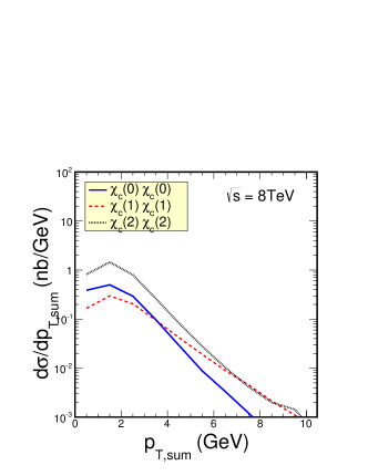
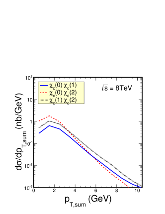
Figure 7: Distributions in the transverse momentum of quarkonium pairs for different spin combinations.

The $\chi_{c}$ mesons radiatively decay into $J/\psi$ mesons. The double feed down leads to a new contribution to the $J/\psi J/\psi$ channel. The direct $J/\psi J/\psi$ contribution is more than order of magnitude larger than the feed-down contribution. However, the $\chi_{c}\chi_{c}$ contribution has its own specificity. In Fig.8 we show distribution in rapidity difference for all $\chi_{c}\chi_{c}$ contributions weighted by branching fractions into $J/\psi$ channel (solid line) compared to the standard direct $J/\psi J/\psi$ contribution (dashed line). At large rapidity difference the feed-down contribution dominates over the contribution of the standard mechanism. Here we assumed that the $J/\psi$’s from the decay will be collinear to their parent $\chi_{c}$’s. How important is the feed-down contribution for different experimental situations will be discussed elsewhere paperJPsi .

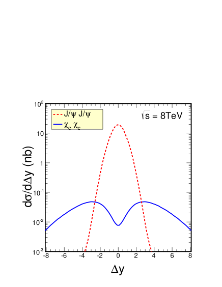
Figure 8: Distributions in the rapidity difference between two $J/\psi$ (dashed line) and for the sum over all $\chi_{c}\chi_{c}$ combinations multiplied by combined branching fractions.

II Conclusions

We have made a first exploratory study of $\chi_{c}$ pair production in proton-proton collisions. The $g^{*}g^{*}\to\chi_{c}(J_{i})\chi_{c}(J_{j})$ amplitudes for off-shell gluons and different spin combinations $J_{i},J_{j}=0,1,2$ are calculated based on $g^{*}g^{*}\to\chi_{c}(J)$ verticies calculated within the color-singlet nonrelativistic pQCD approach. In this approach the vertices are proportional to the derivative of the spatial wave function at the origin $|R^{\prime}(0)|$. The value of this quantity can be obtained from models of the quarkonia states. Here it has been obtained from the $\chi_{c}(0)\to\gamma\gamma$ branching fraction which was measured experimentally.

We have performed calculations within the $k_{T}$-factorization approach for the $pp\to\chi_{c}\chi_{c}X$ process at $\sqrt{s}=8\,\rm{TeV}$ using Kimber-Martin-Ryskin Kimber:2001sc type unintegrated gluon distribution based on the MSTW2008 MSTW08 collinear gluons.

We have found that the cross sections for different combinations of $\chi_{c}$ quarkonia are of a similar size. The integrated cross sections for different channels are of the order of a few nb. This is of the same order of magnitude as the cross section for $J/\psi$ pair production. This means that a feedown from the double $\chi_{c}$ decays $\chi_{c}\to J/\psi\gamma$ leads to extra nonnegligible contribution which has to be included in the total prompt production of two $J/\psi$ mesons. Due to specific branching fractions the $\chi_{c}(1)\chi_{c}(1)$, $\chi_{c}(1)\chi_{c}(2)$ and $\chi_{c}(2)\chi_{c}(2)$ channels are the dominant ones. The other three contributions can be safly neglected.

The $\chi_{c}\chi_{c}$ contribution to the $J/\psi J/\psi$ final state is interesting but goes beyond the scope of the present analysis and will be studied in detail in future dedicated analyses.

The salient feature of the $t$ and $u$-channel gluon exchange mechanism are the broad distributions in rapidity difference $\Delta y$ between $\chi_{c}$ mesons. This is to be contrasted with the narrow $\Delta y$ distribution of $J/\psi$ pairs at leading order. A feed-down from double $\chi_{c}$ production to the double $J/\psi$ channel is therefore expected to be important at large $\Delta y$ and may mimic the kinematical behaviour of double parton scattering mechanisms.

Acknowledgments

We would like to thank Sergey Baranov for discussions and comments on the manuscript. This study was partially supported by the Polish National Science Center grant DEC-2014/15/B/ST2/02528 and by the Center for Innovation and Transfer of Natural Sciences and Engineering Knowledge in Rzeszów.

References

- (1) V. M. Abazov et al. [D0 Collaboration], Phys. Rev. D 90 (2014) no.11, 111101 [arXiv:1406.2380 [hep-ex]].
- (2) V. Khachatryan et al. [CMS Collaboration], JHEP 1409, 094 (2014) doi:10.1007/JHEP09(2014)094 [arXiv:1406.0484 [hep-ex]].
- (3) M. Aaboud et al. [ATLAS Collaboration], Eur. Phys. J. C 77, no. 2, 76 (2017) [arXiv:1612.02950 [hep-ex]].
- (4) R. Aaij et al. [LHCb Collaboration], Phys. Lett. B 707 (2012) 52 doi:10.1016/j.physletb.2011.12.015 [arXiv:1109.0963 [hep-ex]].
- (5) R. Aaij et al. [LHCb Collaboration], JHEP 1706 (2017) 047 Erratum: [JHEP 1710 (2017) 068] [arXiv:1612.07451 [hep-ex]].
- (6) S. P. Baranov, Phys. Rev. D 84 (2011) 054012.
- (7) S. P. Baranov, A. M. Snigirev, N. P. Zotov, A. Szczurek and W. Schäfer, Phys. Rev. D 87 (2013) no.3, 034035 [arXiv:1210.1806 [hep-ph]].
- (8) R. Aaij et al. [LHCb Collaboration], JHEP 1310 (2013) 115 [arXiv:1307.4285 [hep-ex]].
- (9) S. Chatrchyan et al. [CMS Collaboration], Eur. Phys. J. C 72 (2012) 2251 [arXiv:1210.0875 [hep-ex]].
- (10) G. Aad et al. [ATLAS Collaboration], JHEP 1407 (2014) 154 [arXiv:1404.7035 [hep-ex]].
- (11) P. Hagler, R. Kirschner, A. Schäfer, L. Szymanowski and O. V. Teryaev, Phys. Rev. Lett. 86, 1446 (2001) [hep-ph/0004263].
- (12) B. A. Kniehl, D. V. Vasin and V. A. Saleev, Phys. Rev. D 73 (2006) 074022 [hep-ph/0602179].
- (13) A. K. Likhoded, A. V. Luchinsky and S. V. Poslavsky, Phys. Rev. D 90 (2014) no.7, 074021 [arXiv:1409.0693 [hep-ph]].
- (14) S. P. Baranov, A. V. Lipatov and N. P. Zotov, Phys. Rev. D 93 (2016) no.9, 094012 [arXiv:1510.02411 [hep-ph]].
- (15) A. Cisek and A. Szczurek, EPJ Web Conf. 130 (2016) 05003 doi:10.1051/epjconf/201613005003 [arXiv:1609.08413 [hep-ph]].
- (16) J.-P. Lansberg and Hua-Sheng Shao, Phys. Lett. B751 (2015) 479.
- (17) A. K. Likhoded, A. V. Luchinsky and S. V. Poslavsky, Phys. Rev. D 94 (2016) no.5, 054017 doi:10.1103/PhysRevD.94.054017 [arXiv:1606.06767 [hep-ph]].
- (18) A. K. Likhoded, A. V. Luchinsky and S. V. Poslavsky, Phys. Rev. D 91, no. 11, 114016 (2015) [arXiv:1503.00246 [hep-ph]].
- (19) B. Guberina, J. H. Kühn, R. D. Peccei and R. Rückl, Nucl. Phys. B 174, 317 (1980).
- (20) P. L. Cho and A. K. Leibovich, Phys. Rev. D 53, 150 (1996) [hep-ph/9505329].
- (21) P. L. Cho and A. K. Leibovich, Phys. Rev. D 53, 6203 (1996) [hep-ph/9511315].
- (22) R. S. Pasechnik, A. Szczurek and O. V. Teryaev, Phys. Rev. D 78, 014007 (2008) [arXiv:0709.0857 [hep-ph]].
- (23) R. S. Pasechnik, A. Szczurek and O. V. Teryaev, Phys. Lett. B 680, 62 (2009) [arXiv:0901.4187 [hep-ph]].
- (24) R. S. Pasechnik, A. Szczurek and O. V. Teryaev, Phys. Rev. D 81, 034024 (2010) [arXiv:0912.4251 [hep-ph]].
- (25) K.A. Olive et al. (Particle Data Group), Chin. Phys. C38 (2014) 090001.
- (26) M. A. Kimber, A. D. Martin and M. G. Ryskin, Phys. Rev. D 63 (2001) 114027 [hep-ph/0101348].
- (27) A.D. Martin, W.J. Stirling, R.S. Thorne, and G. Watt, Eur.Phys.J. C 63, 189 (2009).
- (28) A. Cisek, W. Schäfer, A. Szczurek and S. Baranov, a paper in preparation.