Linear-Complexity Relaxed Word Mover’s Distance with GPU Acceleration

Abstract

The amount of unstructured text-based data is growing every day. Querying, clustering, and classifying this big data requires similarity computations across large sets of documents. Whereas low-complexity similarity metrics are available, attention has been shifting towards more complex methods that achieve a higher accuracy. In particular, the Word Mover’s Distance (WMD) method proposed by Kusner et al. is a promising new approach, but its time complexity grows cubically with the number of unique words in the documents. The Relaxed Word Mover’s Distance (RWMD) method, again proposed by Kusner et al., reduces the time complexity from qubic to quadratic and results in a limited loss in accuracy compared with WMD. Our work contributes a low-complexity implementation of the RWMD that reduces the average time complexity to linear when operating on large sets of documents. Our linear-complexity RWMD implementation, henceforth referred to as LC-RWMD, maps well onto GPUs and can be efficiently distributed across a cluster of GPUs. Our experiments on real-life datasets demonstrate 1) a performance improvement of two orders of magnitude with respect to our GPU-based distributed implementation of the quadratic RWMD, and 2) a performance improvement of three to four orders of magnitude with respect to our distributed WMD implementation that uses GPU-based RWMD for pruning.

I Introduction

Modern data processing systems should be capable of ingesting, storing and searching across a prodigious amount of textual information. Efficient text search encompasses both a) high quality of the results and b) the speed of execution. Today, the quality of search results is guaranteed by a new class of text representations based on neural networks, such as the popular word2vec representation [1]. The word2vec approach uses neural networks to map words to an appropriate vector space, wherein words that are semantically synonymous will be close to each other. The Word Mover’s Distance (WMD) [2] proposed by Kusner et al. capitalizes on such vector representations to capture the semantic similarity between text documents. WMD is an adaptation of the Earth Mover’s Distance (EMD) [3], first used to measure the similarity between images. Like EMD, WMD constructs a histogram representation of the documents and estimates the cost of transforming one histogram into another. The computational complexity of both approaches scales cubically with the size of the histograms, which makes their application on big data prohibitive.

To mitigate the high complexity of WMD, Kusner et al. proposed using a faster, lower-bound approximation to WMD, called the Relaxed Word Mover’s Distance, or RWMD [2]. They showed that the accuracy achieved by RWMD is very close to that of WMD. According to the original paper, the time complexity of the RWMD method grows quadratically in the size of the histograms, which is a significant improvement with respect to the WMD method. However, the quadratic complexity still limits the applicability of RWMD to relatively small datasets. In practice, computing pairwise similarities across millions of documents has extensive applications in querying, clustering, and classification of text data. This is precisely the focus of our work: to present a new algorithm for computing the Relaxed Word Mover’s Distance that reduces the average time complexity from quadratic to linear. In practice, such a reduction in complexity renders the high-quality search results offered by WMD and RWMD applicable for massive datasets. Additional contributions of this work include:

• A formal complexity and scalability analysis of the LC-RWMD method and other relaxations of WMD.

• Massively parallel GPU implementations and scalable distributed implementations targeting clusters of GPUs.

II Word Mover’s Distance

The Word Mover’s Distance assesses the semantic distance between two documents. If two documents discuss the same topic they will be assigned a low distance even if they have no words in common. WMD consists of two components. The first is a vector representation of the words. The second is a distance measure to quantify the affinity between a pair histograms, wherein each histogram is a bag of words representation of the respective document. The vector representation creates an embedding space, in which semantically synonymous words will be close to each other. This is achieved using word2vec, which maps words in a vector space using a neural network. In fact, word2vec uses the weight matrix of the hidden layer of linear neurons as the vector representation of the words from a given vocabulary.

The distance between two documents is calculated as the minimum cumulative distance of the words from the first document to those of the second document. This optimization problem is well studied in transportation theory and is called the Earth-Mover’s Distance (EMD). Each document is represented as a histogram of words, and each word as a multi-dimensional vector, e.g., under word2vec each word may be represented as a 300-dimensional vector. Fig. 1 depicts the computation of EMD between two histograms.

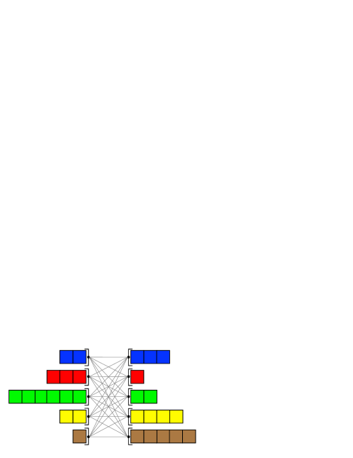
Figure 1: Illustration of Earth Mover’s Distance for two histograms

Given two L1-normalized histograms $x_{1}$ and $x_{2}$, where $\sum_{p}x_{1}[p]=\sum_{q}x_{2}[q]=1.0$, and a cost matrix $c$, EMD tries to discover a flow matrix $y$ that minimizes the cost of moving $x_{1}$ into $x_{2}$. Formally, EMD is computed as follows:

$$\text{EMD}(x_{1},x_{2})=\min\sum_{p,q}y[p,q]c[p,q]\quad\text{s.t.}$$

$$y[p,q]\geq 0,\quad\sum_{q}y[p,q]=x_{1}[p],\quad\sum_{p}y[p,q]=x_{2}[q],$$

where $y[p,q]$ indicates how much of word $p$ in $x_{1}$ has to flow to word $q$ in $x_{2}$, and $c[p,q]$ indicates the unit cost of moving word $p$ in $x_{1}$ to word $q$ in $x_{2}$.

The combination of word embeddings and EMD forms the core of the WMD distance measure. In [2], WMD was shown to outperform seven state-of-art baselines in terms of the $k$-nearest-neighbor classification error across several text corpora. This is because WMD captures linguistic similarities of semantic and syntactic nature and learns how different writers may express the same viewpoint or topic, irrespective of whether they use same words.

III Complexity of WMD and Its Relaxations

Assume that we are given two sets of histograms $X_{1}$ and $X_{2}$, and a vocabulary of size $V$. The sets $X_{1}$ and $X_{2}$ can be seen as sparse matrices, wherein each row is a sparse vector of dimension $V$. Each row $X[i]$ represents a histogram that is extracted from a text document and stores the weights (e.g., term frequencies) of the unique words in that document. The popular compressed sparse rows (csr) representation is a convenient way of storing the sparse matrices $X_{1}$ and $X_{2}$.

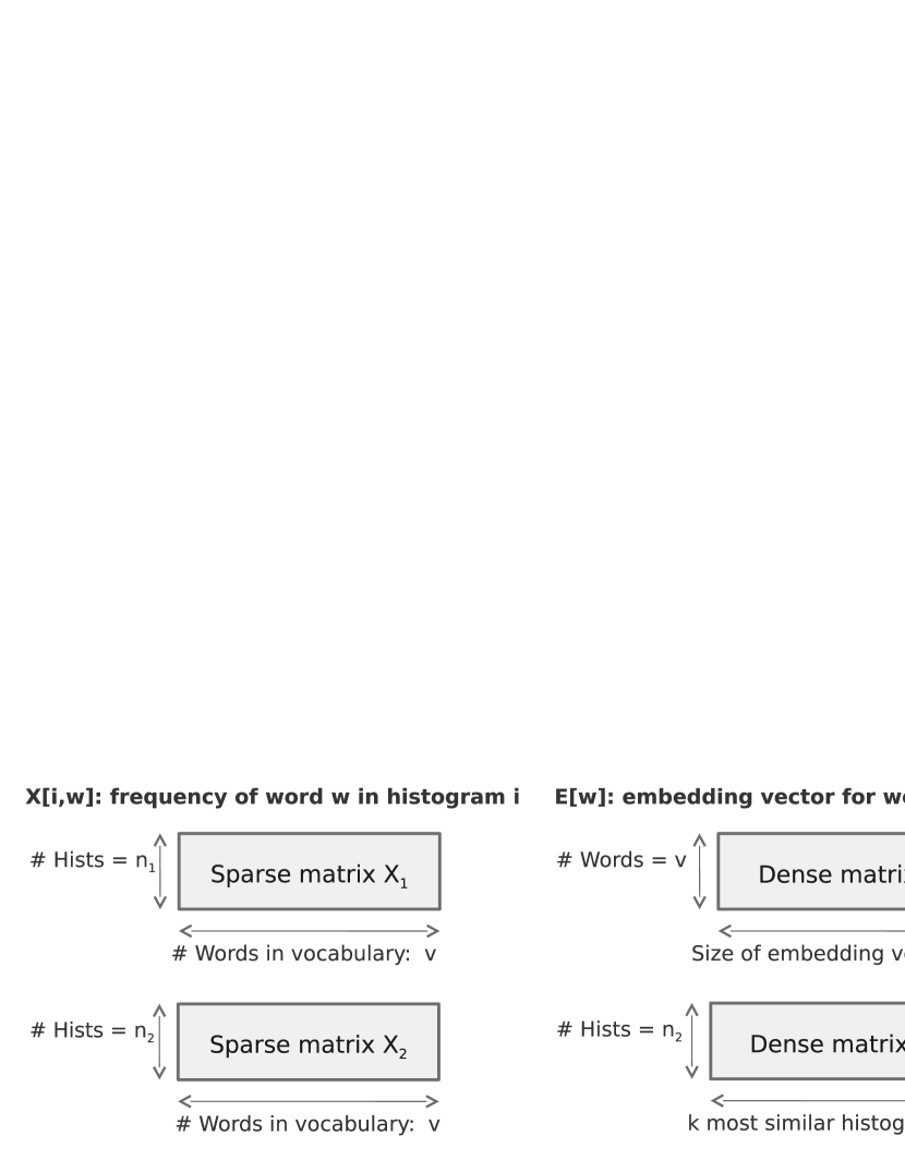
Figure 2: The sparse matrices $X_{1}$ and $X_{2}$ represent two document sets.

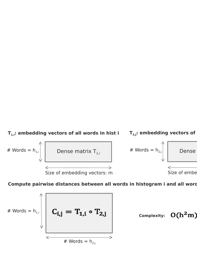
Figure 3: Given two histograms, the first step of WMD is to compute the Euclidean distances between all pairs of words across the two histograms.

Figure 2 shows the input and output data structures of the distance-computation algorithms. Suppose that the sparse matrices $X_{1}$ and $X_{2}$ have $n_{1}$ and $n_{2}$ rows, respectively. Assume that we are also given a dense matrix $E$, which stores embedding vectors for the words that belongs to a given vocabulary. For each word $w\in\{1..V\}$ in the vocabulary, $E[w]$ stores a vector of $m$ floating-point numbers given by some embedding process (word2vec in the case of WMD). Given $X_{1}$, $X_{2}$, and $E$, our goal is to compute the distance between each pair $(X_{1}[i],X_{2}[j])$, $i\in\{1..n_{1}\}$, $j\in\{1..n_{2}\}$, and produce an $n_{1}\times n_{2}$ matrix $D$ of distances.

Typically, a given histogram $X_{2}[j]$ is compared against all $X_{1}[i],i\in\{1..n_{1}\}$, which computes one row of $D$. After that, the top-$k$ smallest distances and the positions of the respective histograms are computed in each row. The top-$k$ results for each row are then stored in an $n_{2}\times k$ matrix $R$.

Given two histograms $X_{1}[i],i\in\{1..n_{1}\}$, and $X_{2}[j],j\in\{1..n_{2}\}$, the first step of WMD is to gather the vector representations of the words in $X_{1}[i]$ and $X_{2}[j]$ from matrix $E$. Assume that the number of nonzeros in $X_{1}[i]$ and $X_{2}[j]$ are $h_{1,i}$ and $h_{2,j}$, respectively. The dense matrix $T_{1,i}$ stores the vector representations of the words in $X_{1}[i]$ and has $h_{1,i}$ rows and $m$ columns. Similarly, the dense matrix $T_{2,j}$ stores the vector representations of the words in $X_{2}[j]$ and has $h_{2,j}$ rows and $m$ columns. Fig. 3 depicts this step.

The Euclidean distances between all pairs of word vectors in $T_{1,i}$ and $T_{2,j}$ form an $h_{1,i}\times h_{2,j}$ dense matrix denoted as $C_{i,j}=T_{1,i}\circ T_{2,j}$. The $\circ$ operation is similar to a matrix multiplication between $T_{1,i}$ and the transpose of $T_{2,j}$, but instead of computing dot products between the word vectors, Euclidean distances are computed. The complexity of the $\circ$ operation across two matrices, each with $O(h)$ rows and $O(m)$ columns, is the same as the complexity of a matrix multiplication operation and is given by $O(h^{2}m)$.

Solving the WMD problem: Suppose that for each $X_{1}[i],i\in\{1..n_{1}\}$, a dense vector $F_{1,i},i\in\{1..n_{1}\}$ is constructed in which only the nonzeros of $X_{1}[i]$ are stored. The size of $F_{1,i}$ is then $h_{1,i}$. Similarly, suppose that for each $X_{2}[j],j\in\{1..N_{2}\}$, a dense representation $F_{2,j},i\in\{1..N_{2}\}$ is constructed in which only the nonzeros of $X_{2}[j]$ are stored. The size of $F_{2,j}$ is then $h_{2,j}$. EMD is computed based on $F_{1,i}$, $F_{2,j}$, and $C_{i,j}=T_{1,i}\circ T_{2,j}$ (see Fig. 4). The notation introduced is summarized in Table I and Table II.

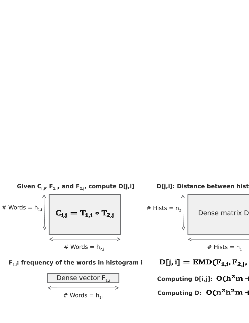
Figure 4: Application of EMD on pairwise distances to compute WMD.

TABLE I: Data structures used in WMD computation

Term	Type	Description
$E$	Input	Embedding vectors for the vocabulary
$X$	Input	A set of histograms (csr matrix)
$T_{i}$	Auxiliary	Embedding vectors for histogram $i$
$F_{i}$	Auxiliary	Term frequencies in histogram $i$
$D$	Output	Distance matrix
$R$	Output	Top-$k$ results

TABLE II: Parameters used in WMD computation

$n$	Number of histograms
$v$	Size of the vocabulary
$m$	Size of the embedding vectors
$h$	Size of a histogram
$k$	Used in top-$k$ calculation

Assuming that the size of $F_{1,i}$ and $F_{2,j}$ is $O(h)$, the complexity of EMD computation is $O(h^{3}\log(h))$. Then, the overall complexity of WMD computation between two pairs of histograms is $O(h^{2}m+h^{3}\log(h))$. If $n_{1}$ and $n_{2}$ are both $O(n)$, the complexity of computing WMD across all pairs of histograms becomes $O(n^{2}h^{2}m+n^{2}h^{3}\log(h))$. So, the complexity of WMD grows quadratically in $n$ (number of documents) and cubically in $h$ (size of histograms).

Solving the RWMD problem: The RWMD provides a lower-bound approximation of the WMD. Similarly to WMD, the first step of RWMD is the computation of $C_{i,j}=T_{1,i}\circ T_{2,j}$, which is a matrix of dimensions $h_{1,i}\times h_{2,j}$. The second step of RWMD is the computation of the minimum value of each row of $C_{i,j}$, which produces a floating-point vector of dimension $h_{1,i}$. The third and final step of RWMD is a dot-product operation between $F_{1,i}$ and the result of the second step, which produces a single floating-point value. Figure 5 illustrates the RWMD computation.

Because the RWMD computation is not symmetric, it is advisable to perform it twice by swapping $T_{1,i}$ with $T_{2,j}$ and $F_{1,i}$ with $F_{2,j}$, and by repeating the previous process. The symmetric lower bound is not necessarily equal to the first, and computation of the maximum of these two bounds provides an even tighter lower bound of WMD. In practice, it is not necessary to compute $T_{2,j}\circ T_{1,i}$ explicitly because this matrix is the transpose of $C_{i,j}=T_{1}[i]\circ T_{2}[j]$, which has already been computed. It is sufficient to compute the minimum value in each column of $C_{i,j}$, and compute a dot product with $F_{2,j}$ to produce the symmetric lower bound.

Finally, the complexity of the overall RWMD computation is determined by the complexity of computing $C_{i,j}$, which is $O(h^{2}m)$. When computed across two sets of size $O(n)$ each, the overall complexity is $O(n^{2}h^{2}m)$, which is significantly lower than the complexity of WMD. However, the complexity of RWMD still grows quadratically with both $n$ and $h$, which can be impractical when $n$ and $h$ are large.

Figure 5: RWMD between histograms $X_{1}[i]$ and $X_{2}[j]$ is the dot-product of the vector $F_{1,i}$ and row-wise minimums of the matrix $C_{i,j}=T_{1,i}\circ T_{2,j}$.

Speeding-up WMD using RWMD: A pruning technique was presented in [2] to speed up the WMD computation, which uses RWMD as a lower bound of WMD. Given a histogram $X_{2}[j]$, first RWMD is computed between $X_{2}[j]$ and all histograms in $X_{1}$. Given a user-defined parameter $k$, the top-$k$ closest histograms in $X_{1}$ are identifed based on the RWMD distances. Next, WMD is computed between $X_{2}[j]$ and the top-$k$ closest histograms in $X_{1}$. The highest WMD value computed by this step provides a cut-off value $L$. WMD is computed between $X_{2}[j]$ and the remaining histograms in $X_{1}$ only if the pairwise RWMD value is lower than $L$. All other histograms will be pruned because they cannot be part of the top-$k$ results of WMD. A small $k$ leads to a small $L$, and hence, a more effective pruning.

Word Centroid Distance: Another approximation of WMD is Word Centroid Distance (WCD), wherein a single vector, called the centroid, is computed for each histogram $X[i]$ by multiplying $X[i]$ by $E$ [2]. This operation, essentially, computes a weighted average of all the embedding vectors associated with the words that are in $X[i]$. The WCD between two histograms $X_{1}[i]$ and $X_{2}[j]$ is given by the Euclidean distance between the respective centroids. The complexity of computing all centroids is then $O(nhm)$ and the complexity of computing all distances across two sets of size $O(n)$ each is $O(n^{2}m)$. When $n>>h$, the overall complexity becomes $O(n^{2}m)$. Although WCD has a low complexity, it is not a tight lower bound of WMD. Thus, it is not suitable when a high accuracy is required.

IV Linear-Complexity RWMD

A main disadvantage of the quadratic-complexity RWMD method is that it may compute the distances between the same pair of words $O(n^{2})$ times. This overhead could be eliminated completely by precomputing the distances between all possible pairs of words in the vocabulary. However, such an approach would require $O(v^{2})$ memory space, which typically is prohibitive. Typical vocabulary sizes are on the order of a few million terms, which could, for instance, include company or person names in a business analytics setting. Storing distances across millions of terms requires tens of terabytes of storage space. In addition, accesses to this storage would be random, rendering software parallelization and hardware acceleration impractical.

Second, even if the distances across all words in the vocabulary are pre-computed and stored in a large and fast storage medium that enables parallel random accesses, if a given word $w$ appears in all histograms $X_{1}[i],i\in\{1..n_{1}\}$, the quadratic-complexity RWMD method would have to compute the word that is closest to $w$ in a given histogram $X_{2}[j]$ exactly $n_{1}$ times. Such a redundancy, again leads to a quadratic time complexity when this computation is repeated for all histograms $X_{2}[j],j\in\{1..n_{2}\}$.

We describe a new method for computing RWMD that addresses both of the aforementioned problems and reduces the time complexity to linear. Even though our approach may redundantly compute the distance between the same pair of words up to $n_{2}$ times, it entails a very low space complexity. In fact, our approach not only reduces the computational complexity with respect to the straightforward RWMD method, but also reduces the space complexity significantly. Because it requires a limited amount of working memory, it is very suitable for hardware acceleration. Lastly, our approach maps well onto the linear algebra primitives supported by modern GPU programming infrastructures.

Reducing the time complexity of RWMD from quadratic to linear makes it possible to compute pairwise distances across 1) large sets of documents (millions of documents) and 2) large histograms (millions of entries in histograms). We have implemented the new technique and showed that it is the only practical way of computing RWMD between all pairs across millions of documents, which leads to trillions of RWMD computations. Notably, we have measured a performance improvement of two orders of magnitude with respect to the quadratic-complexity RWMD method.

The focal point of our work is a novel decomposition of the RWMD computation into two phases, with each phase having linear complexity in terms of the size of the histograms in $X_{1}$ and $X_{2}$. For a given histogram $X_{2}[j],j\in\{1..n_{2}\}$, the first phase computes the Euclidean distance to the closest entry in histogram $X_{2}[j]$ for each word in the vocabulary, which produces $Z$, a dense floating-point vector of dimension $v$ (see Fig. 6 for illustration). The second phase performs a sparse-matrix dense-vector multiplication between $X_{1}$ and $Z$, which produces the RWMD between all $X_{1}[i],i\in\{1..n_{1}\}$ and $X_{2}[j]$ (see Fig. 7 for illustration).

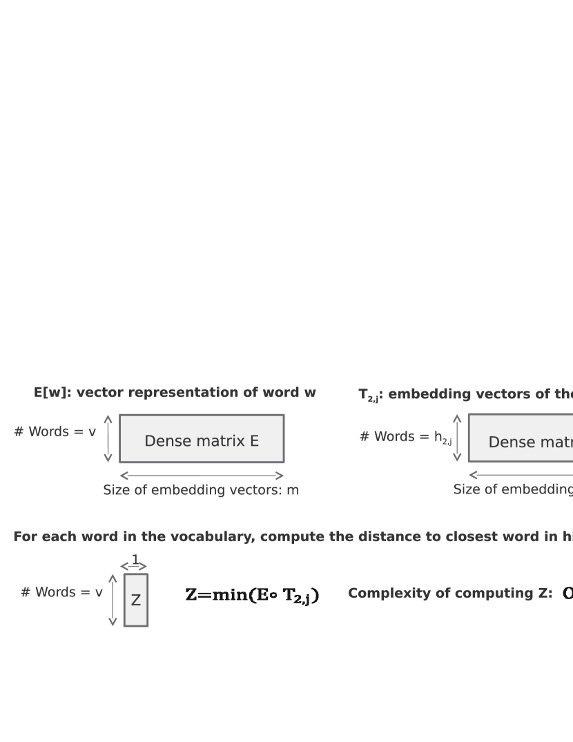
Figure 6: Linear-Complexity RWMD: First phase.

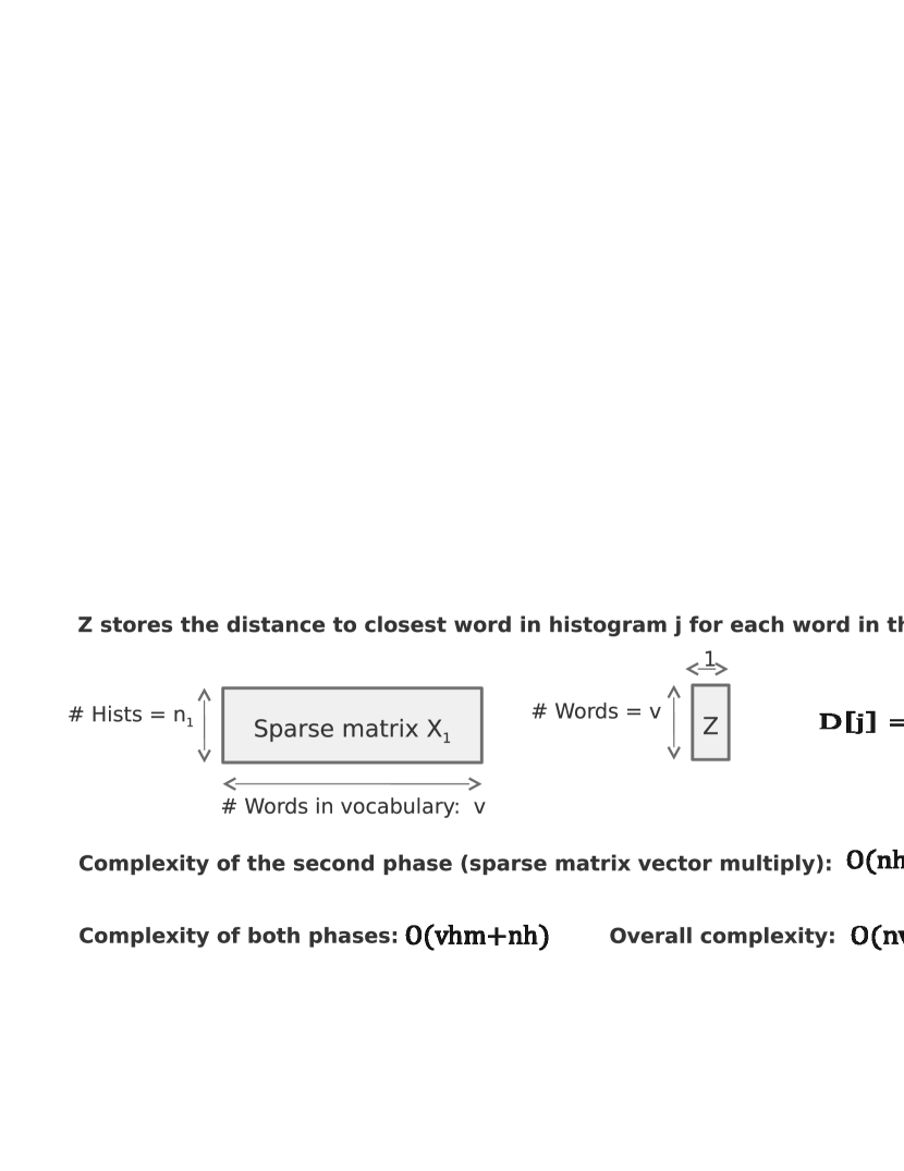
Figure 7: Linear-Complexity RWMD: Second phase.

The first phase is similar to the quadratic-complexity RWMD implementation given in Section III in that it treats the vocabulary as a single histogram and computes pairwise Euclidean distances across all words in the vocabulary and the words in a given histogram $X_{2}[j]$ by computing $E\circ T_{2}[j]$. Next, row-wise minimums are computed to derive the minimum distances between the words in the vocabulary and the words in $X_{2}[j]$, and the results are stored in the vector $Z$ of size $v$. The complexity of this phase is determined by the $\circ$ operation and is given by $O(vhm)$.

In the second phase, $X_{1}$ is multiplied by $Z$ to compute the RWMD. This phase is essentially a sparse-matrix dense-vector multiplication operation. For each $X_{1}[i],i\in\{1..n_{1}\}$, this phase gathers the minimum distances from $Z$ based on the positions of the words in $X_{1}[i]$ and then computes a dot-product with $F_{1,i}$. Therefore, the overall functionality is equivalent to the quadratic-complexity RWMD given in Section III. Note that the second phase computes distances across all histograms in $X_{1}$ and a single histogram from $X_{2}$ in parallel, hence its time complexity is $O(nh)$. A main advantage of our method is that the relatively high cost of the first phase is amortized over a large number of histograms $X_{1}[i],i\in\{1..n_{1}\}$ in the second phase.

The overall complexity of the linear complexity RWMD (LC-RWMD) algorithm when comparing a single histogram from $X_{2}$ against all histograms in $X_{1}$ is then $O(vhm+nh)$. The overall complexity when comparing all histograms of $X_{2}$ against all histograms of $X_{1}$ is $O(nvhm+n^{2}h)$. When $n$ and $v$ are of the same complexity, the overall complexity becomes $O(n^{2}hm)$. Even though this complexity still grows quadratically with the number of histograms (i.e., $n$), it grows linearly with the size of the histograms (i.e., $h$).

The algorithm described so far computes the costs of moving histograms $X_{1}[i],i\in\{1..n_{1}\}$ to histograms $X_{2}[j],j\in\{1..n_{2}\}$. Assume that these results are stored in an $n_{2}\times n_{1}$ matrix $D_{1}$. To achieve a tight lower bound for WMD, the costs of moving the histograms $X_{2}[j],j\in\{1..n_{2}\}$ to $X_{1}[i],i\in\{1..n_{1}\}$, also have to be computed. Therefore, after computing $D_{1}$ in full, we swap $X_{2}$ and $X_{1}$, and run the LC-RWMD algorithm once more, which produces an $n_{1}\times n_{2}$ matrix $D_{2}$. The final distance matrix $D$ is produced by computing the maximum values of the symmetric entries in $D_{1}$ and $D_{2}$ (i.e., $D=\max(D_{1},D_{2}^{T})$).

When $O(n)=O(v)$, our approach reduces the average complexity of computing RWMD between a pair of histograms from $O(h^{2}m)$ to $O(hm)$. Such a reduction makes LC-RWMD orders of magnitude faster than the straightforward RWMD. When $O(n)\neq O(v)$, the reduction in complexity is given by $min(nh/v,hm)$, which is typically determined by the first term, i.e., $nh/v$. Thus, LC-RWMD has significant advantages when the size of the histograms $h$ is large or the number of histograms $n$ is larger than the size of the vocabulary (i.e., $v$). Therefore, an important optimization we have in our LC-RWMD implementation is to eliminate the words that do not appear in $X_{1}$ from the vocabulary. Similarly, when $X_{1}$ and $X_{2}$ are swapped, the words that do not appear in $X_{2}$ are eliminated.

Many-to-many LC-RWMD: The LC-RWMD technique described so far compares a single histogram from one set with all histograms from another set. Although this approach is very fast when both sets are very large, it does not offer similar benefits when one or both sets are small in size. In particular, comparing an $X_{2}[j],j\in\{1..n_{2}\}$ with all $X_{1}[i],i\in\{1..n_{1}\}$ may not use the available compute resources in full if $n_{1}$ is not large enough. To circumvent this problem, we have developed a many-to-many implementation of LC-RWMD, wherein several histograms from $X_{2}[j],j\in\{1..n_{2}\}$ are compared with all $X_{1}$ concurrently.

Assume, for simplicity, that all $n_{2}$ histograms from $X_{2}$ are compared with all $n_{1}$ histograms from $X_{1}$ in parallel. In this case, the first phase of the LC-RWMD algorithm computes $E\circ T_{2}$, where all $T_{2}[j],j\in\{1..n_{2}\}$ are combined in a single matrix $T_{2}$ with $O(n_{2}h)$ rows and $m$ columns. Afterwards, row-wise minima of $E\circ T_{2}$ are computed separately for each $j\in\{1..n_{2}\}$, which produces a $Z$ matrix of dimension $v\times n_{2}$. Next, the second phase of the LC-RWMD algorithm simply mulltiplies the $n_{1}\times v$ sparse matrix $X_{1}$ with $Z$ to produce an $n_{1}\times n_{2}$ distance matrix. In practice, it is not necessary to compute all $n_{1}\times n_{2}$ distances in a single pass of the algorithm, but the set $X_{2}$ can be divided into smaller batches that can be compared with all $X_{1}$ concurrently.

V GPU implementations

We have developed GPU-accelerated and distributed implementations of our linear-complexity RWMD algorithm as well as the more straightforward quadratic-complexity approach, and demonstrated excellent scalability for both.

Figure 8 depicts the GPU implementation of the quadratic-complexity RWMD method detailed in Section III. Here, we parallelize the computation of a complete column of the pairwise distance matrix $D$ by storing all $T_{1,i},i\in\{1..n_{1}\}$ matrices in the GPU memory, and by performing pairwise RWMD computations across all $T_{1,i},i\in\{1..n_{1}\}$ and a single $T_{2,j},j\in\{1..n_{2}\}$ at once. The RWMD computations are performed using an adaptation of the implementation given in Section III. The Euclidean distance computations across all $T_{1,i},i\in\{1..n_{1}\}$ matrices and a single $T_{2,j},j\in\{1..n_{2}\}$ are performed by combining all $T_{1,i},i\in\{1..n_{1}\}$ in a single matrix $T_{1}$ with $O(nh)$ rows and $m$ columns, and by using NVIDIA’s CUBLAS library for multiplying it with $T_{2,j}$. The row-wise and column-wise minimum operations are performed using NVIDIA’s Thrust library. The dot-product operations are performed using CUBLAS again. Such an implementation requires $O(nhm)$ space in the GPU memory because each $T_{1,i}$ matrix requires $O(hm)$ space, and we store $O(n)$ such matrices simultaneously in the GPU memory.

Figure 8: Mapping the Quadratic-Complexity RWMD method to GPU.

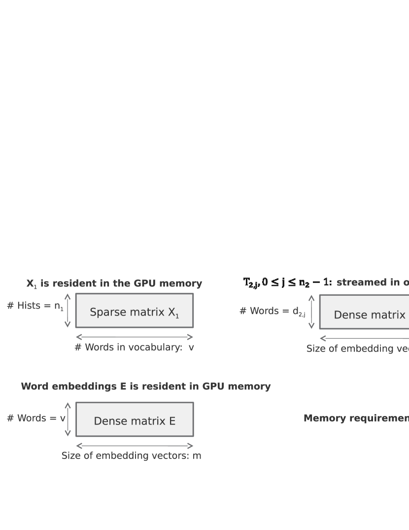
Figure 9: Mapping the Linear-Complexity RWMD method to GPU.

Fig. 9 shows the GPU implementation of the linear complexity RWMD method detailed in Section III. In the first phase, our implementation uses the CUBLAS library for computing Euclidean distances between $E$ and a single $T_{2,j},j\in\{1..n_{2}\}$, and then the Thrust library for computing row-wise minima. In the second step, we use NVIDIA’s CUSPARSE library for multiplying $X_{1}$ by the result of the first phase. Unlike the quadratic-complexity implementation, the linear-complexity RWMD does not store $T_{1,i},i\in\{1..n_{1}\}$, matrices in the GPU memory. Instead of allocating the dense $T_{1}$ matrix that stores embedding vectors for all words in all histograms in $X_{1}$, LC-RWMD simply stores the sparse matrix $X_{1}$, which requires $O(nh)$ space, and the embedding vectors for the complete vocabulary (i.e., $E$), which requires $O(vm)$ space. Therefore, the overall space complexity of LC-RWMD is $O(nh+vm)$. When $O(v)=O(n)$, the overall space complexity becomes $O(nh+nm)$. As a result, the space complexity of LC-RWMD is smaller than that of the quadratic-complexity RWMD by a factor of $min(h,m)$. In conclusion, LC-RWMD reduces not only the time complexity by a factor of $h$ with respect to the straightforward RWMD, but also the space complexity by a similar factor. Table III summarizes these results.

TABLE III: Complexity Comparison

	Time Complexity	Space Complexity
LC-RWMD	$O(nvhm+n^{2}h)$	$O(nh+vm)$
RWMD	$O(n^{2}h^{2}m)$	$O(nhm)$
Reduction	$O(min(nh/v,hm))$	$O(min(nh/v,m))$

All our algorithms are data-parallel and can easily be distributed across several GPUs. Spreading either $X_{1}$ or $X_{2}$ across several GPUs is sufficient. The only function that may require communication in distributed setting is the top-$k$ computation. However, the associated communication cost is typically marginal compared with the cost of computation.

VI Performance Evaluation

Table IV summarizes the characteristics of the datasets used in our experiments in terms of the number of documents ($n$) and the average number of unique words per document excluding the stop-words, which indicates the average histogram size ($h$). Both datasets are proprietary and used in our production systems for news classification.

TABLE IV: Characteristics of the datasets used in experiments

Dataset	$n$	$h$ (average)	$v_{e}$
Set 1	1M	107.5	452,058
Set 2	2.8M	27.5	292,492

Our algorithms require two datasets for comparison. The first set $X_{1}$ is resident (i.e., fixed) and the second set $X_{2}$ is transient (i.e., unknown). In our experiments, we treat the datasets given in Table IV as resident sets. Given a second set of documents (i.e., $X_{2}$), we compare it with $X_{1}$. In typical use cases, $X_{1}$ and $X_{2}$ are completely independent sets, e.g., one is the training set and the other is the test set. However, in the experiments presented, we define $X_{2}$ to be a randomly sampled subset of $X_{1}$ for the sake of simplicity.

The experiments presented in this section use embedding vectors generated by word2vec [1] on Google News, where the vocabulary size is three million words (i.e., $v=3,000,000$), and each word vector is composed of 300 single-precision floating-point numbers (i.e., $m=300$). However, the number of embedding vectors the LC-RWMD algorithm stores in the GPU memory is given by the number of unique words that exist in the resident dataset. We call this number $v_{e}$, and show the respective values in Table IV.

We deployed our algorithms on a cluster of four IBM POWER8+ nodes, where each node had two-socket CPUs with 20 cores and 512 GB of CPU memory. Each node had four NVIDIA Tesla P100 GPUs attached via NVLINK interfaces. A P100 GPU has 16 GB of memory, half of which we used to store the resident data structures, and the rest for the temporary data structures. The POWER8+ nodes were connected via 100 Gb Infiniband interfaces. All our code is written in C++. We used version 14.0.1 of IBM’s XL C/C++ compiler to build our code, CUDA 8.0 to program the GPUs, and MPI for inter-node and inter-process communication.

Figure 10 shows the ratio of overlap between the top-$k$ results of WMD and the top-$k$ results of RWMD. The line labeled WMD (1%) indicates the ratio of the top-$k$ results of the RWMD that overlap with the top 1% results of WMD, where $k$ is determined based on the percentage given on the $x$-axis. Figure 10 shows that the ratio of overlap varies between 0.72 and 1 for RWMD, and proves that RWMD is a high-quality aproximation of WMD. The same analysis is performed between WCD and WMD in Fig. 11, where we observe overlap ratios that are as low as 0.13, indicating that WCD is not a high-quality approximation of WMD.

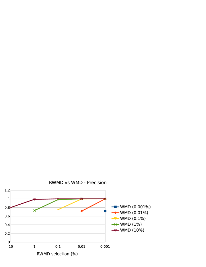
Figure 10: Amount of overlap between top-$k$ results of RWMD and WMD.

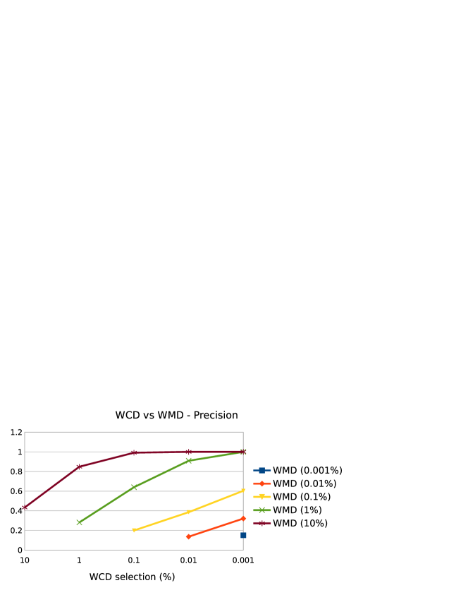
Figure 11: Amount of overlap between top-$k$ results of WCD and WMD.

Figure 12 and Figure 13 compare LC-RWMD, the quadratic-complexity RWMD, and WMD in terms of the runtime performance. Figure 12 shows the average time to compute the distance between a single transient histogram and one million resident histograms from Set 1. Similarly, Fig. 13 shows the average time to compute the distance between a single transient histogram and 2.8 million resident histograms from Set 2. We observe that LC-RWMD is faster than straightforward RWMD by approximately a factor of $h$. Notably, when running LC-RWMD on a single GPU, the time to compute one million distances is around 120 ms for Set 1. For Set 2, which has smaller histograms, 2.8 million distances can be computed in approximately only 160 ms.

Both the straightforward RWMD and the LC-RWMD benefit from parallelization on multiple GPUs. Both are data-parallel algorithms and demonstrate linear scaling as we increase the number of GPUs used. Notably, the time to compare one transient document against all resident documents is approximately 8 ms for Set 1 and 10 ms for Set 2 when running LC-RWMD on 16 GPUs. We distribute either the resident dataset or the transient dataset across multiple GPUs. In the case of the straightforward RWMD, the storage requirements are much higher per histogram, and hence, fewer histograms can be fit into the GPU memory. When the complete resident set does not fit into the GPU memory, the resident histograms are copied into the GPU memory in several batches, which creates additional overhead. To minimize this overhead, we distributed the resident set when multiple GPUs were available. For instance, when using 16 GPUs, the complete Set 2 data fits into the distributed GPU memory, and the copy overheads are completely eliminated, which results in a super-linear speedup for the straightforward RWMD as shown in Fig. 13. The LC-RWMD uses more compact data structures, enabling the complete resident set to be stored in the memory of a single GPU. When several GPUs are available, it is advisable to replicate the smaller set and distribute the larger set for LC-RWMD.

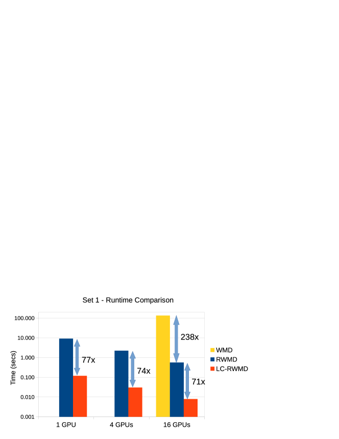
Figure 12: Time to compare a single document with 1M documents.

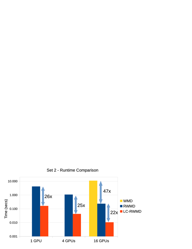
Figure 13: Time to compare a single document with 2.8M documents.

Figure 12 and Figure 13 also show the runtime results for WMD, which are approximately two orders of magnitude higher than those of the quadratic-complexity RWMD. In this work, we developed a parallel WMD implementation that distributes the resident dataset across several CPU processes, wherein each CPU process owns a dedicated GPU that performs the Euclidean distance and RWMD computations. In addition, we implemented the pruning algorithm described in Section III to significantly reduce the number of EMD computations. Each CPU process then runs the state-of-the-art EMD library [4] on its share of the resident data independently. Note that in the pruning algorithm, the top-$k$ results computed by RWMD helps derive a cut-off value. Figure 12 and Figure 13 show the average runtime results for WMD for $k=128$ when using 16 CPU processes and 16 GPUs controlled by those processes. Of course, using a smaller $k$ value reduces the time to compute WMD. For instance, when using $k=16$, the time our algorithms took to compute the WMD dropped by a factor of three for each set. Nevertheless, when computing WMD, we had to use very small transient sets (a few hundred documents from Set 1 and a few thousand documents from Set 2, randomly sampled) to make the WMD computation tractable.

Figure 14 evaluates the suitability of WMD and LC-RWMD for $k$-nearest-neighbors classification, where the $x$-axis indicates $k$ and the $y$-axis indicates the precision at top-$k$. Here we used the fully labeled Set 2, where we organized the labels into four subsets: those that have 300 to 1000 examples are part of the small subset, those that have 1000 to 10,000 examples are in the medium subset, those that have 10,000 to 100,000 examples are in the large subset and those that have 100,000 to one million examples are in the very large subset. For each document, we computed the fraction of the documents that have the same label in its top-$k$ list. For each $k$, we averaged these results within the same label, and then computed the geometric mean across different labels within the same subset. The results indicate that the precision achieved by LC-RWMD is very close to that of WMD for small sets. However, for large sets, WMD becomes intractable. The results also indicate that the precision is a function of the size of the datasets. Thus, there is a real need for scalable algorithms, such as LC-RWMD.

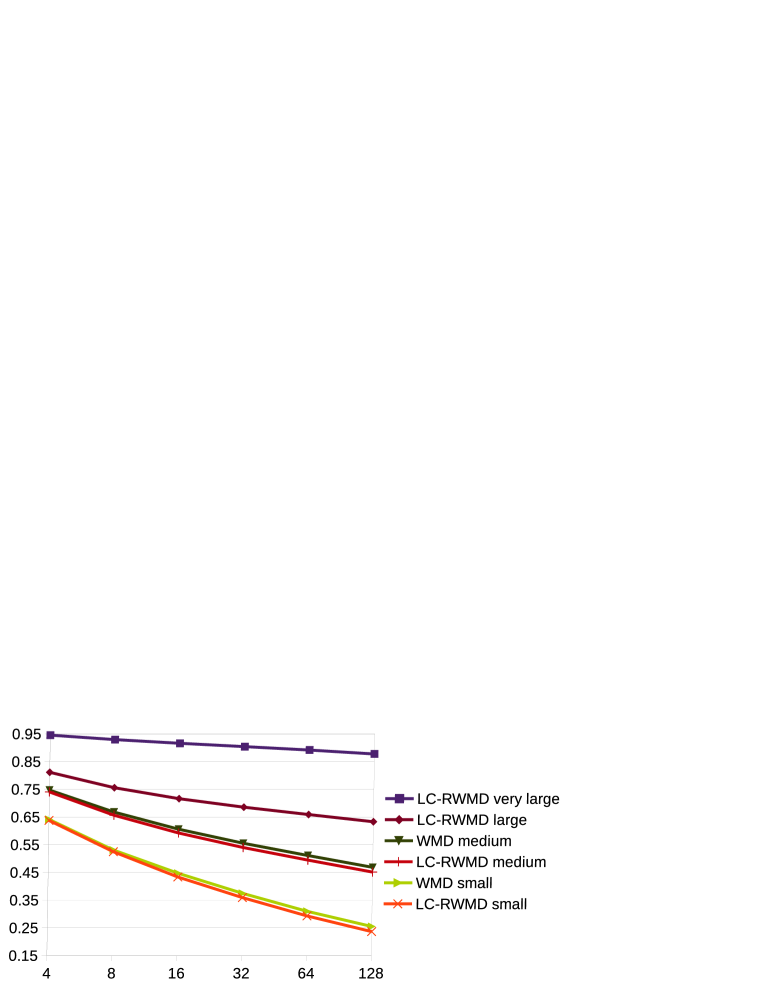
Figure 14: WMD vs LC-RWMD: Precision at top-$k$ for Set 2.

VII Related Work

Several methods have been proposed to achieve lower bounds for EMD that will reduce the time to answer nearest-neighbor queries [5, 6, 7, 8, 9, 10, 11]. Those lower bounds can be used in multi-step query architectures in which an initial filter step is followed by a refinement step. Significant scalability has been observed, especially when the lower bounds are such that they can be used by an index structure. In these approaches, the speedup is achieved by an efficient pruning of the potential candidates. Nevertheless, in very large sets, the number of remaining candidates that the EMD has to be computed on is still big enough to be prohibitive. Alternatively, a compressed representation of the documents can be used to compute EMD fast, but approximately [12]. Another approximate EMD computation algorithm has been proposed in the image-processing domain, which notably achieves linear time complexity [13] using a wavelet-based approach. However, whether the algorithm proposed in [13] can be extended to compute WMD is an open research problem.

To the best of our knowledge, the above-mentioned techniques have not been directly used in the computation of the WMD. However, some lower bounds of the WMD have been introduced in [2]. For instance, the Word Centroid Distance provides a fast and scalable lower bound and can be used to facilitate the pruning in a nearest-neighbor query. RWMD is a tighter lower bound of WMD, but its quadratic time complexity presents scalability issues (see Section III).

Recently, Huang et al. proposed a supervised version of the WMD algorithm that can improve the accuracy of distance computation with respect to the original unsupervised WMD algorithm [14]. The LC-RWMD algorithm proposed by this work is also unsupervised, but can be extended to support supervision. The relaxation technique used by Huang et al. in [14] relies on Cuturi’s Sinkhorn Distance algorithm [15], which has quadratic time complexity. Therefore, it is not as scalable as the LC-RWMD algorithm.

VIII Conclusion

The Relaxed Word Mover’s Distance (RWMD) was proposed by Kusner et al. in their seminal paper as a tight lower bound for the popular Word Mover’s Distance. However, Kusner et al. proposed a quadratic-complexity implementation of RWMD. In this work, we show that the Relaxed Word Mover’s Distance can be implemented in linear time on average when computing distances across large sets of documents. We then show a practical implementation of our method, which maps well onto commonly used dense and sparse linear algebra routines, and can be executed efficiently on GPUs. In addition, we demonstrate that our implementations can be efficiently scaled out across several GPUs and exhibit a perfect strong or weak scaling behavior.

IX Acknowledgement

We thank Dr. Nikolas Ioannou from IBM Research for his technical comments and Ms. Charlotte Bolliger from IBM Research for her language-related corrections.

References

- [1] Tomas Mikolov, Kai Chen, Greg Corrado, and Jeffrey Dean. Efficient estimation of word representations in vector space. CoRR, abs/1301.3781, 2013.
- [2] Matt J. Kusner, Yu Sun, Nicholas I. Kolkin, and Kilian Q. Weinberger. From word embeddings to document distances. In Proc. ICML, pages 957–966, 2015.
- [3] Yossi Rubner, Carlo Tomasi, and Leonidas J Guibas. A metric for distributions with applications to image databases. In Proc. ICCV, pages 59–66. IEEE, 1998.
- [4] Ofir Pele and Michael Werman. Fast Earth Mover’s Distance (EMD) Code, 2013. http://www.ariel.ac.il/sites/ofirpele/FastEMD/code/.
- [5] Ira Assent, Marc Wichterich, Tobias Meisen, and Thomas Seidl. Efficient similarity search using the earth mover’s distance for large multimedia databases. In Proc. ICDE, pages 307–316. IEEE, 2008.
- [6] Jia Xu, Zhenjie Zhang, Anthony KH Tung, and Ge Yu. Efficient and effective similarity search over probabilistic data based on earth mover’s distance. Proceedings of the VLDB Endowment, 3(1-2):758–769, 2010.
- [7] Brian E Ruttenberg and Ambuj K Singh. Indexing the earth mover’s distance using normal distributions. Proceedings of the VLDB Endowment, 5(3):205–216, 2011.
- [8] Marc Wichterich, Ira Assent, Philipp Kranen, and Thomas Seidl. Efficient emd-based similarity search in multimedia databases via flexible dimensionality reduction. In Proc. ICMD, pages 199–212. ACM, 2008.
- [9] Jia Xu, Jiazhen Zhang, Chao Song, Qianzhen Zhang, Pin Lv, Taoshen Li, and Ningjiang Chen. Emd-dsjoin: Efficient similarity join over probabilistic data streams based on earth mover’s distance. In Proc. APWeb, pages 42–54. Springer, 2016.
- [10] Jin Huang, Rui Zhang, Rajkumar Buyya, Jian Chen, and Yongwei Wu. Heads-join: Efficient earth mover’s distance similarity joins on hadoop. IEEE Transactions on Parallel and Distributed Systems, 27(6):1660–1673, 2016.
- [11] Jin Huang, Rui Zhang, Rajkumar Buyya, and Jian Chen. Melody-join: Efficient earth mover’s distance similarity joins using mapreduce. In Proc. ICDE, pages 808–819. IEEE, 2014.
- [12] Merih Seran Uysal, Daniel Sabinasz, and Thomas Seidl. Approximation-based efficient query processing with the earth mover’s distance. In Proc. DASFAA, pages 165–180, New York, NY, USA, 2016. Springer-Verlag New York, Inc.
- [13] Sameer Shirdhonkar and David W. Jacobs. Approximate earth mover’s distance in linear time. In Proc. CVPR, 2008.
- [14] Gao Huang, Chuan Guo, Matt J. Kusner, Yu Sun, Fei Sha, and Kilian Q. Weinberger. Supervised word mover’s distance. In Proc. NIPS, pages 4862–4870, 2016.
- [15] Marco Cuturi. Sinkhorn distances: Lightspeed computation of optimal transport. In Proc. NIPS, pages 2292–2300, 2013.