Single flavour filtering for RHMC in BQCD

Abstract

Filtering algorithms for two degenerate quark flavours have advanced to the point that, in 2+1 flavour simulations, the cost of the strange quark is significant compared with the light quarks. This makes efficient filtering algorithms for single flavour actions highly desirable, in particular when considering 1+1+1 flavour simulations for QED+QCD. Here we discuss methods for filtering the RHMC algorithm that are implemented within BQCD, an open-source Fortran program for Hybrid Monte Carlo simulations.

1 Introduction

While the lattice QCD community has achieved dynamical simulations at or near the physical pion mass Aoki:2008sm ; Durr:2008zz ; Durr:2010vn ; Durr:2010aw , the Monte Carlo generation of gauge field configurations with light quarks presents a numerically intensive challenge, and is only possible for groups with access to primary tier supercomputing resources. After several decades, the Hybrid Monte Carlo (HMC) algorithm Duane:1987de remains the method of choice for dynamical QCD simulations.

The leading expense in modern dynamical simulations is due to the fermion determinant. To enable the use of Monte Carlo methods, the Grassmannian fields which represent the quarks are integrated out analytically,

$$\prod_{f}\int D\psi_{f}D\overline{\psi}_{f}\,\exp\left[-\overline{\psi}_{f}M_{f}\psi_{f}\right]=\prod_{f}\det{M_{f}},$$ (1)

where $M_{f}$ is the fermion matrix for the quark flavour $f.$ At this point the resulting fermion matrix determinant can be estimated stochastically through the introduction of pseudofermions,

$$\prod_{f}\det{M_{f}}=\prod_{f}\int D\phi_{f}D\phi_{f}^{*}\,\exp\left[-\phi^{\dagger}_{f}M_{f}^{-1}\phi_{f}\right]$$ (2)

The pseudofermion fields $\phi$ are standard complex numbers and are therefore computable. The simplest pseudofermion formulation is for two degenerate quark flavours,

$$(\det{M})^{2}=\det(M^{\dagger}M)=\int D\phi D\phi^{*}\,\exp\left[-\phi^{\dagger}(M^{\dagger}M)^{-1}\phi\right],$$ (3)

where we have taken advantage of the fact that the determinant of the fermion matrix $M$ is real. In this instance, the determinant is represented by a pseudofermion action with a positive semi-definite matrix,

$$S_{2f}=\phi^{\dagger}K^{-1}\phi,$$ (4)

where $K=M^{\dagger}M.$ The positive semi-definite property enables the generation of pseudofermion fields that satisfy the probability distribution $\rho(\phi)\sim e^{-S_{2f}(\phi)}.$

Single flavour fermion simulations pose additional computational challenges. For Wilson-type actions, the fermion matrix has a complex spectrum, and hence cannot be used directly in the pseudofermion distribution without additional modification. Noting that, if $\det M$ is real and positive we have

$$\det M=\sqrt{\det(M^{\dagger}M)}=\int D\phi D\phi^{*}\,\exp\left[-\phi^{\dagger}(M^{\dagger}M)^{-\frac{1}{2}}\phi\right].$$ (5)

The Rational HMC (RHMC) algorithm Clark:2006fx ; Clark:2006wq solves this problem by replacing the fermion matrix $M$ with a rational approximation to the inverse square root,

$$R(K)\approx K^{-1/2},$$ (6)

where $K=M^{\dagger}M$ is positive semi-definite, such that the pseudofermion action for a single flavour is

$$S_{1f}=\phi^{\dagger}R(K)\phi.$$ (7)

Typically, $R(K)$ is chosen to be the Zolotarev approximation, which is the optimal rational polynomial approximation for $R(z)\simeq z^{-\frac{1}{2}}.$

Due to isospin symmetry being very nearly exact, in pure QCD simulations the up and down quark are almost always chosen to be degenerate. This means that in a $2+1$ flavour simulation only the strange must be treated using RHMC. Historically, the cost of adding the strange quark to a dynamical simulation with already light up and down quarks was relatively small. However, there have been a large number of algorithmic improvements focused on reducing the cost of two flavour simulations, such that in a modern dynamical simulation the cost of the including the strange quark is significant.

Moreover, the precision of lattice QCD calculations of certain quantities has advanced to the point that electromagnetic effects can no longer be neglected, see e.g. Horsley:2015eaa ; Horsley:2015vla ; Borsanyi:2014jba ; Borsanyi:2013lga ; Aoki:2012st . In these QCD+QED calculations, isospin symmetry is explicitly broken as the up and down quarks have different charges $q_{u}\neq q_{d}.$ This means that at the physical point, $1+1+1$ flavour simulations are needed Aoki:2012st , noting that the down and strange quark have different masses $m_{d}\neq m_{s}.$ This motivates us to seek improvements to the single flavour RHMC algorithm that parallel the advances made for the degenerate two flavour case.

2 Filtering algorithms

The essential principle underlying the Hybrid Monte Carlo algorithm is the introduction of a fictitious simulation time co-ordinate, along with the corresponding conjugate momenta and a Hamiltonian describing the evolution in this new simulation time. The molecular dynamics evolution approximately preserves the extended Hamiltonian and this ensures a high acceptance rate for the global Metropolis accept/reject step that takes place at the end of each trajectory.

There are two sources of computational expense in performing simulations at light quark mass. Both stem from the fact that the fermion determinant must be represented stochastically using pseudofermions with a non-local action that features the inverse of the fermion matrix. The first is that the condition number of the fermion matrix increases at light quark mass, causing a large increase in the number of conjugate gradient iterations required to solve the linear system. Solving this system is required at each molecular dynamics step, which means the numerical expense of the inversions is the dominant cost for generating dynamical gauge fields. The second is that the molecular dynamics step-size must be decreased as the quark mass is reduced in order to maintain control over the rapid fluctuations driven by the pseudofermion field.

Splitting the pseudofermion action using a filter provides the opportunity to address both these issues. The application of a filter $F$ to the fermion action kernel $L$ results in a pseudofermion action with multiple terms,

$$\phi^{\dagger}L\phi\rightarrow\phi_{1}^{\dagger}F\phi_{1}+\phi_{2}^{\dagger}F^{-1}L\phi_{2}.$$ (8)

A good choice of filter can have a two fold effect. $F^{-1}$ should act as a preconditioner for $L,$ such that the cost of evaluating the molecular dynamics force is reduced. The second benefit comes from the ability to place the evolution of the two terms on different time scales, such that the expensive fermion matrix inversions are performed less often per trajectory.

There are a number of filtering techniques Kamleh:2011dc ; Hasenbusch:2001ne ; Urbach:2005ji ; AliKhan:2003br ; Luscher:2003vf ; Luscher:2005rx that have been developed for two flavour simulations, two of which are most relevant to this discussion. Polynomial filtering Kamleh:2011dc uses a polynomial approximation to the inverse as a preconditioner for $L,$ with the advantage that a short polynomial filter can simultaneously capture the high frequency dynamics whilst being cheap to evaluate. Utilising appropriately factored polynomials allows for additional time scales to be introduced. Mass preconditioning Hasenbusch:2001ne ; Urbach:2005ji uses the lattice Dirac matrix at heavier value of the quark mass parameter as a filter, and again it is possible to create a tiered molecular dynamics integration scheme by using successively increasing values of the hopping parameter $\kappa,$ with simulations at the physical quark mass using four or more Hasenbuch terms. The possibility of combining mass preconditioning and polynomial filtering was recently shown to remove the need to fine tune the Hasenbuch parameter(s) Haar:2016bwe .

In this work we propose two classes of filter that can be applied to the Rational Hybrid Monte Carlo action,

$$S_{RHMC}=\phi^{\dagger}R(K)\phi.$$ (9)

Analogously to the two flavour case, we can construct a polynomial filter for RHMC by choosing a low order polynomial $P(K)\simeq K^{-1/2}$ that approximates the inverse square root, such that

$$S_{PF-RHMC}=\phi_{1}^{\dagger}P(K)\phi_{1}+\phi_{2}^{\dagger}P(K)^{-1}R(K)\phi_{2}.$$ (10)

Given a class of polynomials $P(K)$, such as the Chebyshev approximations, we only need to tune the polynomial order $p.$ The polynomial term $P(K)$ is cheap to evaluate. So long as the roots of $P(K)$ are sufficiently away from zero then we can obtain the filtered rational polynomial $P(K)^{-1}R(K)$ needed for the remainder term with minimal additional expense by using a multi-shift solver, and the filter will reduce the force associated with the remainder term such that it can be placed on a coarser integration scale.

Table 1: The coefficients for the Zolotarev rational approximation to the inverse square root $R(z^{2})$ given by equation (11), optimised for the range $z\in[5\times 10^{-5},3]$ with rational polynomial order $n=20.$

$k$	$a_{k}$	$b_{k}$
1	$9.563244545350\times 10^{+01}$	$2.185152657378\times 10^{+01}$
2	$8.388503498802\times 10^{+00}$	$3.869255332779\times 10^{+00}$
3	$1.938402066167\times 10^{+00}$	$1.011688743145\times 10^{+00}$
4	$5.393711779563\times 10^{-01}$	$2.908314285103\times 10^{-01}$
5	$1.577758224234\times 10^{-01}$	$8.587639032804\times 10^{-02}$
6	$4.682604103557\times 10^{-02}$	$2.555797860752\times 10^{-02}$
7	$1.395718122336\times 10^{-02}$	$7.624224868005\times 10^{-03}$
8	$4.165459337102\times 10^{-03}$	$2.275977093976\times 10^{-03}$
9	$1.243636491310\times 10^{-03}$	$6.795636775098\times 10^{-04}$
10	$3.713408528751\times 10^{-04}$	$2.029168564071\times 10^{-04}$
11	$1.108828440206\times 10^{-04}$	$6.059122761302\times 10^{-05}$
12	$3.310947727642\times 10^{-05}$	$1.809210191033\times 10^{-05}$
13	$9.885863174458\times 10^{-06}$	$5.401564705966\times 10^{-06}$
14	$2.951119430158\times 10^{-06}$	$1.612073222848\times 10^{-06}$
15	$8.803512407386\times 10^{-07}$	$4.805018241491\times 10^{-07}$
16	$2.620044683831\times 10^{-07}$	$1.426073879295\times 10^{-07}$
17	$7.736439845055\times 10^{-08}$	$4.171524002026\times 10^{-08}$
18	$2.224004044081\times 10^{-08}$	$1.160749939012\times 10^{-08}$
19	$5.815072459290\times 10^{-09}$	$2.682241760431\times 10^{-09}$
20	$1.029675478286\times 10^{-09}$	$2.352768004344\times 10^{-10}$
$d_{n}=6.411915162135\times 10^{-02}$

The second type of filter we propose is based on the observation that the class of Zolotarev rational polynomials $R(K)\simeq K^{-1/2}$ can be written down in an ordered product form,

$$R(K)=d_{n}\prod_{k=1}^{n}\frac{(K+a_{k})}{(K+b_{k}),}$$ (11)

where $a_{k},b_{k},d_{n}>0,$ and the coefficients in the numerator and denominator strictly decrease as $k$ increases such that $a_{k}>a_{k+1},b_{k}>b_{k+1}.$ Table 1 provides the coefficients for the $n=20$ Zolotarev approximation $R(z^{2})$ optimised for the range $z\in[5\times 10^{-5},3]$ as an example. The ordered product can then be partitioned into partial factors Luscher:2012av ; Bruno:2014jqa defined by

$$R_{i,j}(K)=(d_{n})^{\delta_{i,0}}\prod_{k=i+1}^{j}\frac{(K+a_{k})}{(K+b_{k})},$$ (12)

where the overall coefficient $d_{n}$ is only present if $i=0.$ The value of this partitioning is revealed when we observe that truncations of the ordered product $R_{0,t}(K)$ at order $t<n$ also provide an approximation to the inverse square root,

$$R_{0,t}(K)=d_{n}\prod_{k=1}^{t}\frac{(K+a_{k})}{(K+b_{k})}\simeq K^{-1/2}.$$ (13)

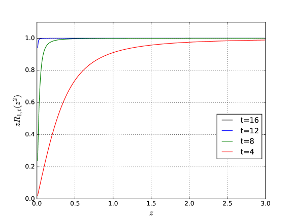
Figure 1: The function $zR_{0,t}(z^{2})\simeq 1$ for various values of the truncation order $t.$ The truncated products $R_{0,t}$ derive from a Zolotarev rational polynomial $R(z^{2})\simeq 1/\sqrt{z^{2}}$ of order $n=20$ over the range $z\in[5\times 10^{-5},3].$ The graph demonstrates that truncations of the ordered product also approximate the inverse square root.

This property is demonstrated in Figure 1, where we plot the functions $zR_{0,t}(z^{2})\simeq 1$ for $z>0,$ where $R_{0,t}$ are the truncations of the $n=20$ Zolotarev approximation specified in Table 1. We see that for all choices of $t$ the approximation is good at large values of $z,$ while the range over which the approximation is valid gets successively better as the truncation order $t$ increases. We observe at $t=16$ the approximation error is negligible over almost the entire range of $z.$ Hence we have shown that truncations of the ordered product successfully capture the high frequency dynamics. Next we consider the correction term which is simply the remaining factors associated with a given truncation order $t,$

$$R_{t,n}(K)=\prod_{k=t+1}^{n}\frac{(K+a_{k})}{(K+b_{k})}\simeq 1.$$ (14)

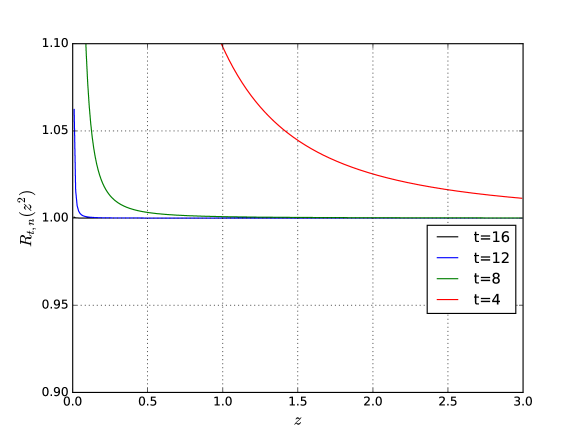
Figure 2: The correction term $R_{t,n}(z^{2})\simeq 1$ for various values of the truncation order $t.$ The remainders $R_{t,n}$ derive from a Zolotarev rational polynomial $R(z^{2})\simeq 1/\sqrt{z^{2}}$ of order $n=20$ over the range $z\in[5\times 10^{-5},3].$ The graph demonstrates that truncating the ordered product yields remainders that approximate unity.

Note that, due to the ordering of the product, for values of $k>>1$ we have that $a_{k}\simeq b_{k}$ are both small, and as the order of the polynomials in the numerator and denominator are equal, the correction term is an approximation to unity. This is very clearly demonstrated in Figure 2, which shows the correction terms $R_{t,n}(z^{2})$ arising from different choices of the truncation order $t$ for the Zolotarev approximation from Table 1. The bounds on the vertical axis are set at a 10% deviation from 1. Even at $t=8,$ the correction term is approximately one over a large range, while at $t=16$ the remainder is indistinguishable from unity at the displayed scale. This is significant, as it implies that the correction term will have a correspondingly small molecular dynamics force and thus can be placed on a coarse integration scale.

Based on the above observations, we define the truncated ordered product (top) filtering scheme for RHMC, denoted by tRHMC, such that

$$S_{tRHMC}=\phi_{1}^{\dagger}R_{0,t}(K)\phi_{1}+\phi_{2}^{\dagger}R_{t,n}(K)\phi_{2}$$ (15)

is the tRHMC pseudofermion action. Here we point out a significant advantage of the tRHMC scheme is that, as both terms are simply rational polynomials, it is very easy to implement using preexisting RHMC code.

It is also worth noting that partitioning the ordered product form of the rational polynomial is distinct from partitioning the sum over poles, in which different poles in the expansion of $R(K)$ are simply placed on different time scales. The reason is that the sum over poles simply distributes the inversions based on their expense, and does not share the beneficial properties of the tRHMC scheme mentioned above, namely that by also approximating $K^{-\frac{1}{2}},$ $R_{0,t}$ acts as a high pass filter. A further computational efficiency for the tRHMC scheme may be realised on some hardware architectures due to the memory bandwidth benefits of evaluating multiple small order rational polynomial terms, rather than a single term of full order.

As has been done in the two flavour case, hierarchical filtering schemes can be defined for the single flavour filters that we have proposed. In the case of PF-RHMC, we can add a higher order polynomial $Q(K),(q>p)$ which approximates $P(K)^{-1}K^{-1/2}$ as a secondary filter, which results in the 2PF-RHMC action,

$$S_{2PF-RHMC}=\phi_{1}^{\dagger}P(K)\phi_{1}+\phi_{2}^{\dagger}Q(K)\phi_{2}+\phi_{3}^{\dagger}R(K)[P(K)Q(K)]^{-1}\phi_{3}.$$ (16)

For the tRHMC scheme, we can add a second truncation point in the order product, such that the 2tRHMC action is given by

$$S_{2tRHMC}=\phi_{1}^{\dagger}R_{0,t_{1}}(K)\phi_{1}+\phi_{2}^{\dagger}R_{t_{1},t_{2}}(K)\phi_{2}+\phi_{3}^{\dagger}R_{t_{2},n}(K)\phi_{3}.$$ (17)

3 Characteristic scale tuning

Using a fully generalised integration scheme Kamleh:2011dc ; Haar:2016bwe , it is possible to place each term in the molecular dynamics action on an independent scale. Typically, the step sizes $h_{i}$ associated with a given action term $S_{i}$ can be tuned by force balancing, where given some measure $F_{i}$ of the molecular dynamics forces, for each term we attempt to balance the product of the step size and the force such that $F_{i}h_{i}\sim\mathrm{constant}.$ Here, $F_{i}$ can be the average or maximum force associated with a given term. The maximum tends to prove a better choice, as it is more closely linked with the force variance.

However, in the case of tRHMC, for higher order truncations, the force due to the remainder term is very small. This makes the force-balanced approach to tuning the step sizes unfavourable. Noting that for filtered actions the acceptance rate is primarily determined by the coarsest scale, we adopt an alternative approach to tuning using the characteristic scale. The coarsest scale $h_{0}$ is tuned by fitting the acceptance probability with the complementary error function, $\rho_{\rm acc}\approx\operatorname{erfc}(h_{0}^{2}c^{2}),$ where the characteristic scale $c$ is the only fit parameter. With the coarsest scale $h_{0}$ excluded, the remaining scales $h_{1}>h_{2}>h_{3}\ldots$ are set using the force balancing relation to achieve the target acceptance rate.

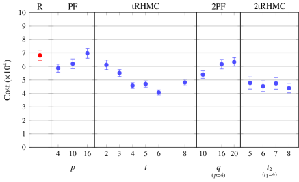
Figure 3: The cost function $C=N_{\rm mat}/\rho_{\rm acc}$ for the different algorithms used in this study. The red point is for vanilla RHMC, while the blue points are for the filtering schemes using characteristic scale tuning. From left to right, first we have the single filter results at various values of their respective order parameters, namely PF-RHMC for different polynomial order $p,$ and tRHMC for different truncation order $t.$ Next we have the two filter results, with 2PF-RHMC at fixed $p=4$ and various $q$ for the polynomial orders, followed by 2tRHMC at fixed $t_{1}=4$ and various $t_{2}$ for the truncation orders.

4 Results

All runs were performed using the open source BQCD software package Nakamura:2010qh ; Haar:2017ubh . Both the PF-RHMC and tRHMC filtering methods are built into the latest release, which is available at the following link:

www.rrz.uni-hamburg.de/services/hpc/bqcd

To compare the different filtering algorithms proposed herein, we start with a thermalised $16^{3}\times 32$ lattice with $N_{f}=2$ flavours of Wilson fermions from a previous study Haar:2016bwe . The Wilson gauge action is used with $\beta=5.6,$ with hopping parameter $\kappa=0.15825,$ providing a pion mass of $m_{\pi}\sim 400\leavevmode\nobreak\ \mathrm{MeV}$ and a lattice spacing of $a\sim 0.08\leavevmode\nobreak\ \mathrm{fm}.$

The various RHMC simulations are then performed with (degenerate) $1+1$ single-flavour pseudofermions. As both flavours are treated equally, they have degenerate force and fermion matrix multiplication count distributions. We tune the step-sizes using the characteristic scale method above such that the acceptance rate $\rho_{acc}\sim 0.75$. The rational polynomial used is the Zolotarev approximation with order $n=20$ and range $[5\times 10^{-5},3]$ given in Table 1. The polynomial filters used in the PF-RHMC runs are the Chebyshev approximations to $K^{-1/2}$ (or $P(K)^{-1}K^{-1/2}$ in the two filter case) with range $[5\times 10^{-5},3]$. The cost function we use to compare our methods is the same as in Haar:2016bwe , namely

$$C=N_{\rm mat}/\rho_{\rm acc},$$ (18)

where the matrix multiplication count $N_{\rm mat}$ is the total for both flavours.

Figure 3 compares the cost function for the various filtering methods described herein. Polynomial-filtered RHMC provides a small benefit over vanilla RHMC. It is clear that tRHMC provides the best performance improvement, at a speedup of around 1.75. The optimal point for tRHMC and 2tRHMC is similar, but the two truncation form is less sensitive to the choice of the truncation parameter.

In summary, we have seen that the tRHMC filtering scheme coupled with characteristic scale tuning works well cross a wide range of truncation orders. The tRHMC algorithm is provided by BQCD, but is also very easy to implement in existing RHMC codes. Multiple truncation filters can be used, and this should prove to be useful at light quark masses. The full details of our study will be published elsewhere.

References

- (1) S. Aoki et al. (PACS-CS), Phys. Rev. D79, 034503 (2009), 0807.1661
- (2) S. Durr et al., Science 322, 1224 (2008), 0906.3599
- (3) S. Durr, Z. Fodor, C. Hoelbling, S.D. Katz, S. Krieg, T. Kurth, L. Lellouch, T. Lippert, K.K. Szabo, G. Vulvert, Phys. Lett. B701, 265 (2011), 1011.2403
- (4) S. Durr, Z. Fodor, C. Hoelbling, S.D. Katz, S. Krieg, T. Kurth, L. Lellouch, T. Lippert, K.K. Szabo, G. Vulvert, JHEP 08, 148 (2011), 1011.2711
- (5) S. Duane, A.D. Kennedy, B.J. Pendleton, D. Roweth, Phys. Lett. B195, 216 (1987)
- (6) M.A. Clark, A.D. Kennedy, Phys. Rev. Lett. 98, 051601 (2007), hep-lat/0608015
- (7) M.A. Clark, PoS LAT2006, 004 (2006), hep-lat/0610048
- (8) R. Horsley et al., J. Phys. G43, 10LT02 (2016), 1508.06401
- (9) R. Horsley et al., JHEP 04, 093 (2016), 1509.00799
- (10) S. Borsanyi et al., Science 347, 1452 (2015), 1406.4088
- (11) S. Borsanyi et al. (Budapest-Marseille-Wuppertal), Phys. Rev. Lett. 111, 252001 (2013), 1306.2287
- (12) S. Aoki et al., Phys. Rev. D86, 034507 (2012), 1205.2961
- (13) W. Kamleh, M. Peardon, Comput. Phys. Commun. 183, 1993 (2012), 1106.5625
- (14) M. Hasenbusch, Phys. Lett. B519, 177 (2001), hep-lat/0107019
- (15) C. Urbach, K. Jansen, A. Shindler, U. Wenger, Comput. Phys. Commun. 174, 87 (2006), hep-lat/0506011
- (16) A. Ali Khan, T. Bakeyev, M. Gockeler, R. Horsley, D. Pleiter, P.E.L. Rakow, A. Schafer, G. Schierholz, H. Stüben (QCDSF), Phys. Lett. B564, 235 (2003), hep-lat/0303026
- (17) M. Lüscher, JHEP 05, 052 (2003), hep-lat/0304007
- (18) M. Lüscher, Comput. Phys. Commun. 165, 199 (2005), hep-lat/0409106
- (19) T. Haar, W. Kamleh, J. Zanotti, Y. Nakamura, Comput. Phys. Commun. 215, 113 (2017), 1609.02652
- (20) M. Luscher, S. Schaefer, Comput. Phys. Commun. 184, 519 (2013), 1206.2809
- (21) M. Bruno et al., JHEP 02, 043 (2015), 1411.3982
- (22) Y. Nakamura, H. Stüben, PoS LATTICE2010, 040 (2010), 1011.0199
- (23) T.R. Haar, Y. Nakamura, H. Stüben, An update on the BQCD Hybrid Monte Carlo program, in Proceedings, 35th International Symposium on Lattice Field Theory (Lattice2017): Granada, Spain, to appear in EPJ Web Conf., 1711.03836