Abstract

We study $6j$-symbols, or Racah coefficients for tensor products of infinite-dimensional unitary principal series representations of the group $\mathrm{SL}(2,\mathbb{C})$. These symbols were constructed earlier by Ismagilov and we rederive his result (up to some slight difference associated with equivalent representations) using the Feynman diagrams technique. The resulting $6j$-symbols are expressed either as a triple integral over complex plane, or as an infinite bilateral sum of integrals of the Mellin-Barnes type.

To the memory of Ludwig Dmitrievich Faddeev

1 Introduction

The problem of decomposition of a tensor product of irreducible representations of classical groups to the direct sum of such representations with the help of $3nj$-symbols is a well known old subject of investigations. Despite of very many results obtained in this field by Clebsch, Gordan, Wigner, van der Waerden, Fock, Racah, Naimark, Biedenharn, and many other researches, it is not completed yet and continues to be developed. In a detailed investigation of the atomic spectra, Racah [23] constructed a closed form expression for $6j$-symbols of finite-dimensional representations of $\mathrm{SU}(2)$ group. It is given by a terminating ${}_{4}F_{3}$ hypergeometric series and determines a set of classical orthogonal polynomials called Racah polynomials [1]. For an outline of the theory of $3nj$-symbols and a list of relevant references, see the handbook [25].

The group $\mathrm{SL}(2,\mathbb{C})$ is one of the most important Lie groups, since it is the smallest rank nonabelian group over the field of complex numbers $\mathbb{C}$ [11]. It coincides with the Lorentz group and therefore its finite-dimensional representations play a crucial role in four-dimensional quantum field theory, since they describe observable elementary particles. Irreducible infinite-dimensional representations of $\mathrm{SL}(2,\mathbb{C})$ also have found appropriate applications in physics. They emerge in a spin chain model that appears in the high-energy regime of quantum chromodynamics, see [17, 18] and [9, 19]. Therefore investigation of the representation theory of this group does not need additional justifications.

This paper is devoted to a consideration of $6j$-symbols, or Racah coefficients (operators) for the tensor product of unitary infinite-dimensional principal series representations of the $\mathrm{SL}(2,\mathbb{C})$ group. The $3j$-symbols, or Clebsch-Gordan coefficients for such representations have been constructed by Naimark long ago [20]. They are defined by a single valued function of three complex variables, describing the representation space, and depend on three integer and three real parameters. The projectors onto irreducible components of the corresponding twofold tensor products are given by integral operators with such kernel functions. Despite of the importance of the problem of building $6j$-symbols for the $\mathrm{SL}(2,\mathbb{C})$ group dealing with threefold tensor products, for the unitary principal series representations they were constructed only recently by Ismagilov in [15, 16].

The previous most close result on this subject was obtained in the work [13], where an integral transform related to the Wilson function was considered and $6j$-symbols for the tensor products involving the unitary principal series representation of the group $\mathrm{SU}(1,1)$ were constructed. The results of Ismagilov open the final chapter of the program of building $3nj$-symbols for the smallest rank groups. As follows from the general $\mathrm{SL}(2,\mathbb{C})$ group representation theory [11], it remains to consider similar problems for the cases involving the complementary series representation, as well as the non-unitary representations. In the present work we rederive the results of Ismagilov using a different approach, namely the Feynman diagrams techniques, and give two different types of integral representations for these $6j$-symbols.

The number of applications of $6j$-symbols is quite large ranging from quantum mechanics, where they describe the angular momentum dynamics, to quantum gravity, statistical mechanics, knot invariants, etc. For instance, the operator intertwining equivalent principal series representations of the $\mathrm{SL}(2,\mathbb{C})$ group (it is described in the next section) plays a crucial role in the construction of general solutions of the vertex type Yang-Baxter equation [5]. In a similar way, the $6j$-symbols considered in this paper should define solutions of a different type Yang-Baxter equation related to IRF (“interaction round a face”) models in statistical mechanics.

In the last decades quantum deformations of the $sl(2)$ algebra have been investigated from various points of view. In particular, the modular double of $U_{q}(sl(2,\mathbb{R}))$ was introduced by Faddeev in [8] and $6j$-symbols for the unitary principal series representation of this algebra have been constructed in [22]. A further extension of these considerations to the simplest quantum supergroup is given in [21]. We expect that our results can be lifted to the complex extension of these quantum groups as well (see [6, 7] for related results).

The paper is organized as follows. In Sect. 2 we outline the structure of $\mathrm{SL}(2,\mathbb{C})$ group and its principal series representation. In Sect. 3 we describe the structure of Clebsch-Gordan coefficients for the tensor product of two such representations and consider their biorthogonality and completeness relations. Sect. 4 contains main results of our work — a new derivation of the Racah coefficients for relevant representations in the form of a kernel of an integral operator relating different bases of threefold tensor products. In Sect. 5 we provide a Mellin-Barnes representation for these $6j$-symbols. In the Appendix we collected some handbook formulae and an auxiliary material.

2 $\mathrm{SL}(2,\mathbb{C})$ group

2.1 Representations of the group and the intertwining operator

Let us describe some basic facts from the representation theory of the group $\mathrm{SL}(2,\mathbb{C})$ [10, 11]. They are formulated in a form that will be natural for dealing with the Racah coefficients and corresponding projection operators.

Usually $\mathrm{SL}(2,\hbox{\bbd C})$ group representations are realized in the space of single-valued functions $\Phi(z,\bar{z})$ on the complex plane, $z\in\mathbb{C}$, with $\bar{z}$ being the complex conjugate of $z$. The non-unitary principal series representation [10] is parameterized by a pair of generic complex numbers $(s,\bar{s})$ subject to the single constraint $2\,(s-\bar{s})\in\mathbb{Z}$. We refer to them as spins in what follows. In order to avoid misunderstanding we emphasize that $s$ and $\bar{s}$ are not complex conjugates of each other. As usual, for a given matrix

$$g=\left(\begin{array}[]{cc}\alpha&\beta\\ \gamma&\delta\\ \end{array}\right)\in\mathrm{SL}(2,\hbox{\bbd C})$$

one can consider $\mathrm{SL}(2,\hbox{\bbd C})$ group action on the two-dimensional plane coordinates $x,y\in\mathbb{C}$ of the form

$$(x,y)\to(x,y)g=(\alpha x+\gamma y,\beta x+\delta y),$$ (1)

or

$$\left({x\atop y}\right)\to g^{-1}\left({x\atop y}\right)=\left({\delta x-\beta y\atop-\gamma x+\alpha y}\right).$$ (2)

If the latter transformation is used then, after denoting $z=y/x$, one comes to the representation $\mathrm{T}^{(s,\bar{s})}$ determined explicitly by the corresponding linear fractional transformation [10]

$$\left[\mathrm{T}^{(s,\bar{s})}(g)\,\Phi\right](z,\bar{z})=\left(\delta-\beta z\right)^{2s}\,\left(\bar{\delta}-\bar{\beta}\bar{z}\right)^{2\bar{s}}\,\Phi\left(\frac{-\gamma+\alpha z}{\delta-\beta z},\frac{-\bar{\gamma}+\bar{\alpha}\bar{z}}{\bar{\delta}-\bar{\beta}\bar{z}}\right).\ \$$ (3)

In [16] Ismagilov used the first option (1) which, after denoting $z=x/y$, yields an equivalent though slightly differently looking representation

$$\left[\mathrm{T}_{a}(g)\,\Phi\right](z,\bar{z})=\left(\beta z+\delta\right)^{a-1}\,\left(\bar{\beta}\bar{z}+\bar{\delta}\right)^{\bar{a}-1}\,\Phi\left(\frac{\alpha z+\gamma}{\beta z+\delta},\frac{\bar{\alpha}\bar{z}+\bar{\gamma}}{\bar{\beta}\bar{z}+\bar{\delta}}\right).$$ (4)

We connect the representation parameters in (3) and (4) as $a=2s+1,\,\bar{a}=2\bar{s}+1$. In [16] the representations are taken to be unitary principal series with the restrictions $a:=m+i\sigma,\;\bar{a}:=-m+i\sigma,\;m\in\hbox{\bbd Z},\;\sigma\in\mathbb{R}.$ In this case one has $a-\bar{a}=2s-2\bar{s}=2m\in 2\mathbb{Z}$, an even integer.

We start our considerations from the general non-unitary representation, which assumes that the representation parameters have the form

$$a=\frac{m}{2}+b+i\sigma,\quad\bar{a}=-\frac{m}{2}+b+i\sigma,\quad m\in\hbox{\bbd Z},\quad b,\sigma\in\mathbb{R}.$$ (5)

The unitary case corresponds to the choice $b=0$ and arbitrary integer $m$. In [16] the following function was used as a representation character

$$\phi_{k}(a,z):=|z|^{i\sigma-m-k}z^{m},\quad k\in\hbox{\bbd Z}.$$

Instead of this notation, we employ the following convention

$$[z]^{a}:=z^{a}\bar{z}^{\bar{a}}=|z|^{2\bar{a}}z^{a-\bar{a}}=|z|^{2b+2i\sigma-m}z^{m},$$

which is a replacement of the function $\phi_{0}(2a,z)$ in [16].

Taking the matrix $g$ lying in a vicinity of the unit matrix, $g=1+\varepsilon\,\mathcal{E}_{ik}$, where $\mathcal{E}_{ik}$ are traceless $2\times 2$ matrices: $(\mathcal{E}_{ik})_{jl}=\delta_{ij}\delta_{kl}-\frac{1}{2}\delta_{ik}\delta_{jl}\,,$ it is not difficult to find generators of the Lie algebra $s\ell(2,\mathbb{C})$ $\mathrm{E}_{ik}$ and $\bar{\mathrm{E}}_{ik}$,

$$\mathrm{T}^{(s,\bar{s})}(1+\varepsilon\,\mathcal{E}_{ik})\,\Phi(z,\bar{z})=\Phi(z,\bar{z})+\left(\varepsilon\,\mathrm{E}_{ik}+\bar{\varepsilon}\,\bar{\mathrm{E}}_{ik}\right)\,\Phi(z,\bar{z})+O(\varepsilon^{2})\,.$$

Explicitly, the generators $\mathrm{E}_{ik}$, $\bar{\mathrm{E}}_{ik}$ are given by the first-order differential operators which we represent as $2\times 2$ matrices $\mathrm{E}^{(s)}$ and $\bar{\mathrm{E}}^{(\bar{s})}$:

$$\mathrm{E}^{(s)}=\left(\begin{array}[]{cc}\mathrm{E}_{11}&\mathrm{E}_{21}\\ \mathrm{E}_{12}&\mathrm{E}_{22}\\ \end{array}\right)=\left(\begin{array}[]{cc}z\partial-s&-\partial\\ z^{2}\partial-2s\,z&-z\partial+s\\ \end{array}\right)=\begin{pmatrix}1&0\\ z&1\end{pmatrix}\begin{pmatrix}-s-1&-\partial\\ 0&s\end{pmatrix}\begin{pmatrix}1&0\\ -z&1\end{pmatrix},$$ (6)

with the matrix $\mathrm{\bar{E}}^{(\bar{s})}$ (yielding the generators $\mathrm{\bar{E}}_{ik}$ in a similar way) obtained from $\mathrm{E}^{(s)}$ after the replacements $z\to\bar{z}\,,\partial\to\bar{\partial}$, and $s\to\bar{s}$.

It is well known that the representations characterized by the parameters $s,\bar{s}$ and $-1-s,-1-\bar{s}$ (or $a,\bar{a}$ and $-a,-\bar{a}$) are equivalent (the values of Casimir operators for them coincide) [11]. There exists an integral operator $\mathrm{M}$ which intertwines such equivalent principal series representations $\mathrm{T}^{(s,\bar{s})}$ and $\mathrm{T}^{(-1-s,-1-\bar{s})}$ for generic complex $s$ and $\bar{s}$,

$$\mathrm{M}(s,\bar{s})\,\mathrm{T}^{(s,\bar{s})}(g)=\mathrm{T}^{(-1-s,-1-\bar{s})}(g)\,\mathrm{M}(s,\bar{s})\,.$$ (7)

Relations (7) can be reformulated as a set of intertwining relations for the Lie algebra generators

$$\mathrm{M}(s,\bar{s})\,\mathrm{E}^{(s)}=\mathrm{E}^{(-1-s)}\,\mathrm{M}(s,\bar{s}),\qquad\mathrm{M}(s,\bar{s})\,\mathrm{\bar{E}}^{(\bar{s})}=\mathrm{\bar{E}}^{(-1-\bar{s})}\,\mathrm{M}(s,\bar{s}).$$ (8)

This $\mathrm{M}$-operator can be written in the following form [10] (for a justification of the taken normalization factor, see [3, 5])

$$\left[\,\mathrm{M}(s,\bar{s})\Phi\,\right](z,\bar{z})=\frac{i^{-|2s-2\bar{s}|}}{\pi}\,\frac{\Gamma\left(s+\bar{s}+|s-\bar{s}|+2\right)}{\Gamma\left(-s-\bar{s}+|s-\bar{s}|-1\right)}\int\mathrm{d}^{2}x\,\frac{\Phi(x,\bar{x})}{[z-x]^{2s+2}},$$ (9)

where $\Gamma(x)$ is the standard gamma function. This is a well-defined operator for generic values of $s$ and $\bar{s}$. Despite of the diverging integral for the discrete values $2s=n,\,2\bar{s}=\bar{n}$, $n,\,\bar{n}\in\mathbb{Z}_{\geq 0}$, it remains well defined in this case too due the appropriate normalizing factor (see the next section).

The described intertwining operator has a meaning of the pseudodifferential operator. Such an interpretation is reached with the help of the following explicit Fourier transformation

$$A(\alpha,\bar{\alpha})\,\int d^{2}z\,\frac{\mathrm{e}^{ipz+i\bar{p}\bar{z}}}{z^{1+\alpha}\bar{z}^{1+\bar{\alpha}}}=p^{\alpha}\bar{p}^{\bar{\alpha}},\qquad\alpha-\bar{\alpha}\in\hbox{\bbd Z},$$ (10)

where the measure is defined as $d^{2}z=dxdy=\frac{i}{2}dzd\bar{z}$ (with $z=x+iy$, $\bar{z}=x-iy$) and the normalization constant has the canonical form [10]

$$A(\alpha,\bar{\alpha}):=\frac{i^{-|\alpha-\bar{\alpha}|}}{\pi}\,\frac{\Gamma\left(\frac{\alpha+\bar{\alpha}+|\alpha-\bar{\alpha}|+2}{2}\right)}{\Gamma\left(\frac{-\alpha-\bar{\alpha}+|\alpha-\bar{\alpha}|}{2}\right)}.$$ (11)

For non-integer values of $\alpha$ the form of this constant can be simplified

$$A(\alpha,\bar{\alpha})=\frac{i^{\bar{\alpha}-\alpha}}{\pi a(\alpha+1)},\qquad a(\alpha):=\frac{\Gamma(1-\bar{\alpha})}{\Gamma(\alpha)},$$ (12)

which can be checked by substitution of the relation $\alpha=\bar{\alpha}+m,\,m\in\mathbb{Z},$ for general non-unitary principal series representation and application of the reflection formula for the gamma function.

Let us replace in formula (10) the complex variables $p$ and $\bar{p}$ by differential operators, $p\to i\partial_{x}$ and $\bar{p}\to i\partial_{\bar{x}}$. Then one can use the standard finite-difference operator $\mathrm{e}^{a\partial_{x}}f(x)=f(x+a)$ in order to set by definition

$$\left(i\partial_{z}\right)^{\alpha}\left(i\partial_{\bar{z}}\right)^{\bar{\alpha}}\Phi(z,\bar{z}):=A(\alpha,\bar{\alpha})\,\int d^{2}x\,\frac{\Phi(x,\bar{x})}{[z-x]^{1+\alpha}},$$ (13)

$$\makebox[0.0pt]{}[z-x]^{1+\alpha}:=(z-x)^{1+\alpha}(\bar{z}-\bar{x})^{1+\bar{\alpha}},\quad\alpha-\bar{\alpha}\in\mathbb{Z}.$$ (14)

The constraint on the exponents $\alpha,\bar{\alpha}$ in (14) ensures that the function $[z-x]^{\alpha}$ is single-valued. If one takes the separate holomorphic part, then it has a branch cut, but a special choice of the antiholomorphic multiplier yields the single-valued function. It is this pseudodifferential operator that is used for fixing the normalizing factor in the intertwining operator (9) – one simply sets $\mathrm{M}(s,\bar{s}):=\left[i\partial_{z}\right]^{2s+1}$. In particular, for $s=\bar{s}=-1/2$ one has $\mathrm{M}(s,\bar{s})=\hbox{{1}\kern-2.5pt\hbox{l}}$ (the unit operator), see [10].

2.2 Decoupling of the finite-dimensional representations

The fact that finite-dimensional representations can be derived from the general principal series representation by the reduction is well known [11, 3]. Indeed, for the discrete set $2s=n,\,2\bar{s}=\bar{n}$, $n,\,\bar{n}\in\mathbb{Z}_{\geq 0}$, the integral operator (9) becomes a finite order differential operator $\left(i\partial_{z}\right)^{n+1}\left(i\partial_{\bar{z}}\right)^{\bar{n}+1}$. This follows not from the formal identification $\mathrm{M}(s,\bar{s})=\left[i\partial_{z}\right]^{2s+1}$, but from the rigorous consideration of singularities of meromorphic functions of $s$ appearing after the action of this operator on sufficiently smooth functions $\Phi(z,\bar{z})$ (9) and careful consideration of the limits $2s\to n,\,2\bar{s}\to\bar{n}$, see in [10] a description of the tempered distribution $z^{-n-2}{\bar{z}}^{-\bar{n}-2}$. The main transformation law (3) implies that for such discrete values of spins an $(n+1)(\bar{n}+1)$-dimensional representation decouples from the general infinite-dimensional one. This is evident, since the $(n+1)(\bar{n}+1)$-dimensional vector space spanned by polynomials $z^{k}\bar{z}^{\bar{k}}$, $k=0,1,\cdots,n$ and $\bar{k}=0,1,\cdots,\bar{n}$, is invariant with respect to the action of the operators $\mathrm{T}^{(s,\bar{s})}(g)$.

This picture is nicely captured by the intertwining operator $\mathrm{M}(s,\bar{s})$ (9). One can introduce a single generating function for these basis polynomials $[z-x]^{n}=(z-x)^{n}(\bar{z}-\bar{x})^{\bar{n}}$, where $x$, $\bar{x}$ are some auxiliary variables. Clearly the series expansion of $[z-x]^{n}$ in $x$ and $\bar{x}$ yields needed vectors $z^{k}\bar{z}^{\bar{k}}$,$k=0,1,\cdots,n$, $\bar{k}=0,1,\cdots,\bar{n}$. Then from relation (7) it follows that the space annihilated by the operator $\mathrm{M}(s,\bar{s})$ (the null-space) is invariant under the action of the operators $\mathrm{T}^{(s,\bar{s})}(g)$. Therefore any nontrivial invariant null-space yields a sub-representation. For $2s=n$ and $2\bar{s}=\bar{n}$, the intertwining operator turns into the differential operator $\partial^{n+1}\bar{\partial}^{\bar{n}+1}$ which annihilates the generating function $[z-x]^{n}$. However, the full null-space includes all harmonic functions, i.e. it is much bigger. The image of the intertwining operator $\mathrm{M}(-1-s,-1-\bar{s})$ is invariant under the action of $\mathrm{T}^{(s,\bar{s})}(g)$, which follows from formula (7). We have also the relation

$$\left[\,\mathrm{M}(-1-s,-1-\bar{s})\Phi\,\right](z,\bar{z})=\frac{i^{-|2s-2\bar{s}|}}{\pi}\,\frac{\Gamma\left(-s-\bar{s}+|s-\bar{s}|\right)}{\Gamma\left(s+\bar{s}+|s-\bar{s}|+1\right)}\int d^{2}x\,(z-x)^{2s}(\bar{z}-\bar{x})^{2\bar{s}}\,\Phi(x,\bar{x}).$$ (15)

After dropping the numerical factor $\Gamma\left(-s-\bar{s}+|s-\bar{s}|\right)$ diverging for $2s=n$ and $2\bar{s}=\bar{n}$, we clearly see that the image of $\mathrm{M}(-1-s,-1-\bar{s})$ is a polynomial of $z$ and $\bar{z}$ forming the needed finite-dimensional subspace. So, the polynomial finite-dimensional subspace is formed as an intersection of the null-space of $\mathrm{M}(s,\bar{s})$ and the image of the properly normalized operator $\mathrm{M}(-1-s,-1-\bar{s})$ with the spins $2s=n$ and $2\bar{s}=\bar{n}$.

The fact that the intertwining operator annihilates the generating function $[z-x]^{n}$ can be established using the inversion property of the intertwining operator. Indeed, the notation $\mathrm{M}(s,\bar{s})=\left[i\partial_{z}\right]^{2s+1}$ and $\mathrm{M}(-1-s,-1-\bar{s})=\left[i\partial_{z}\right]^{-1-2s}$ formally suggests that $\mathrm{M}(s,\bar{s})\,\mathrm{M}(-1-s,-1-\bar{s})=\hbox{{1}\kern-2.5pt\hbox{l}}$. However, this relation cannot be true for positive integer values of the spins. Let us rewrite this inversion relation after substituting the explicit forms of the kernels for integral operators $\mathrm{M}(-1-s,-1-\bar{s})$ (15) and 1l (given by the Dirac delta-function)

$$\left[i\partial_{z}\right]^{2s+1}[z-x]^{2s}=\pi i^{|2s-2\bar{s}|}\frac{\Gamma\left(s+\bar{s}+|s-\bar{s}|+1\right)}{\Gamma\left(-s-\bar{s}+|s-\bar{s}|\right)}\,\delta^{2}(z-x).$$ (16)

For $2s\to n,\,2\bar{s}\to\bar{n},\,n,\bar{n}\in\hbox{\bbd Z}_{\geq 0},$ the multiplier in the denominator $\Gamma\left(-s-\bar{s}+|s-\bar{s}|\right)$ acquires the poles. For $n\geq\bar{n}$ it is $\Gamma(-\bar{n})$ and for $n\leq\bar{n}$ it is $\Gamma(-n)$, so that the right-hand side of this relation vanishes. Therefore, $\left[i\partial_{z}\right]^{n+1}[z-x]^{n}=0,\;n,\bar{n}=0,1,2,\ldots,$ i.e. the generating function of the finite-dimensional representations $[z-x]^{n}$ is the kernel function of the properly normalized operator $\mathrm{M}(-1-n/2,-1-\bar{n}/2)$.

3 Decomposition of the tensor product of two representations

Decomposition of the tensor product of two principal series representations to irreducible components has been constructed by Naimark [20]. The projection operator

$$\mathrm{T}_{a_{1}}\otimes\mathrm{T}_{a_{2}}\xrightarrow{\mathrm{P}(a_{1},a_{2}|a_{3})}\mathrm{T}_{a_{3}},$$

is given by the following integral operator

$$\Phi(z_{1},z_{2})\xrightarrow{\mathrm{P}(a_{1},a_{2}|a_{3})}\left[\mathrm{P}(a_{1},a_{2}|a_{3})\,\Phi\right](z_{3})=\int\mathrm{d}^{2}\,z_{1}\mathrm{d}^{2}\,z_{2}\,W\left({a_{1},a_{2},a_{3}\atop z_{1},z_{2},z_{3}}\right)\,\Phi(z_{1},z_{2})\,.$$

The kernel function represents the Clebsch-Gordan coefficients and has the following exlpicit form

$$W\left({a_{1},a_{2},a_{3}\atop z_{1},z_{2},z_{3}}\right)=[z_{2}-z_{1}]^{-\frac{1+a_{1}+a_{2}+a_{3}}{2}}[z_{3}-z_{1}]^{-\frac{1+a_{1}-a_{2}-a_{3}}{2}}[z_{2}-z_{3}]^{-\frac{1-a_{1}+a_{2}-a_{3}}{2}},$$ (17)

which coincides with the expression given by Naimark in [20] after the identification $z_{3}=z$. This function is fixed up to an overall normalization constant by the requirement of covariance

$$\left[\beta z_{3}+\delta\right]^{a_{3}-1}\left[\mathrm{P}(a_{1},a_{2}|a_{3})\,\Phi\right]\left(\frac{\alpha z_{3}+\gamma}{\beta z_{3}+\delta}\right)$$

$$\makebox[5.0pt]{}=\int\mathrm{d}^{2}\,z_{1}\mathrm{d}^{2}\,z_{2}\,W\left({a_{1},a_{2},a_{3}\atop z_{1},z_{2},z_{3}}\right)\,\left[\beta z_{1}+\delta\right]^{a_{1}-1}\,\left[\beta z_{2}+\delta\right]^{a_{2}-1}\Phi\left(\frac{\alpha z_{1}+\gamma}{\beta z_{1}+\delta},\frac{\alpha z_{2}+\gamma}{\beta z_{2}+\delta}\right).$$ (18)

The $3j$-symbols (17) were derived in [20] for unitary principal series representations. However, we stress that the corresponding derivation does not depend on whether the parameter $i\sigma$ is purely imaginary or a general complex number. Therefore formulas (17), (18) are true for general non-unitary principal series representation with $b\neq 0$ in the parametrization of spin variables (5). It should be noticed that in formula (17) one has the exponent of the form $\alpha:=\frac{1+a_{1}+a_{2}+a_{3}}{2}$ and similar ones which do not preserve the general restriction on spin values $\alpha-\bar{\alpha}\in\hbox{\bbd Z}$. As pointed out in [20], this means that the nontrivial Clebsch-Gordan coefficients exist only in the cases when the integers $m_{1},m_{2},m_{3}$ entering the definition of parameters $a_{1},a_{2},a_{3}$ satisfy the constraint that $m_{1}+m_{2}+m_{3}$ is an even integer (in [15, 16] this condition was resolved by forcing all $m_{j}$ to be even integers).

In an infinitesimal form the global relation (18) is equivalent to the system of defining equations

$$\left(\mathrm{E}^{(-a_{1})}_{z_{1}}+\mathrm{E}^{(-a_{2})}_{z_{2}}+\mathrm{E}^{(a_{3})}_{z_{3}}\right)W\left({a_{1},a_{2},a_{3}\atop z_{1},z_{2},z_{3}}\right)=0.$$ (19)

Here for brevity we use the superscript $a_{j}=2s_{j}+1$ for labeling the generators instead of the previously used $s_{j}$-variables, in terms of which equivalent representations are described by the reflection $s_{j}\to-s_{j}-1$.

Now we present the basic elements of the diagram technique which will be used throughout the paper. The kernels of integral operators are represented in the form of two-dimensional Feynman diagrams. The propagator is given by the following expression

$$\frac{1}{[z-w]^{\alpha}}\equiv\frac{1}{(z-w)^{\alpha}(\bar{z}-\bar{w})^{\bar{\alpha}}}=\frac{(\bar{z}-\bar{w})^{\alpha-\bar{\alpha}}}{|z-w|^{2\alpha}}=\frac{(-1)^{\alpha-\bar{\alpha}}}{[w-z]^{\alpha}},$$ (20)

where $\alpha-\bar{\alpha}$ is an integer. It is depicted on the diagrams by the lint with the arrow directed from point $w$ to $z$ with the index $\alpha$ corresponding to scaling exponents. The diagrammatic representation for our main building block $W\left({a_{1},a_{2},a_{3}\atop z_{1},z_{2},z_{3}}\right)$ is given by Fig. 1. We have the diagram with three external vertices and due to the required behavior under $\mathrm{SL}(2,\mathbb{C})$-transformations (18) this diagram coincides up to an overall coefficient with the simple conformal triangle. The name “conformal triangle” is due to the fact that the system of equations (19) coincides with the set of Ward identities for the three-point conformal invariant Green function in two-dimensional conformal field theory [2].

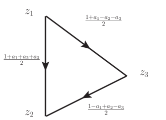
Figure 1: Diagrammatic representation of $W\left({a_{1},a_{2},a_{3}\atop z_{1},z_{2},z_{3}}\right)$.

For the unitary principal series representation, which corresponds to the choice $b=0$ in (5), the complex conjugation is equivalent to the change of signs of all spin variables:

$$\overline{W\left({a_{1},a_{2},a_{3}\atop z_{1},z_{2},z_{3}}\right)}=W\left({-a_{1},-a_{2},-a_{3}\atop z_{1},z_{2},z_{3}}\right).$$ (21)

From now on we shall assume that the function $\overline{W}$ (21) is a complex conjugate of $W$. The representations with the parameters $a$ and $-a$ are known to be equivalent. Therefore function (21) is the Clebsch-Gordan coefficient for the decomposition problem when all three involved representations are replaced by the equivalent ones.

The kernel of the dual projection operator $\mathrm{T}_{a_{3}}\xrightarrow{\mathrm{P}(a_{3}|a_{1},a_{2})}\mathrm{T}_{a_{1}}\otimes\mathrm{T}_{a_{2}},$ is determined precisely by the function (21)

$$\Phi(z_{3})\xrightarrow{\mathrm{P}(a_{3}|a_{1},a_{2})}\left[\mathrm{P}(a_{3}|a_{1},a_{2})\,\Phi\right](z_{1},z_{2})=\int\mathrm{d}^{2}\,z_{3}\,W\left({-a_{1},-a_{2},-a_{3}\atop z_{1},z_{2},z_{3}}\right)\,\Phi(z_{3})\,.$$

This follows from the biorthogonality relation considered in the next section.

3.1 Orthogonality and completeness

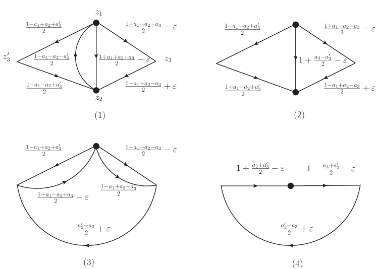
Figure 2: (1) The initial regularized orthogonality diagram. (2) The diagram after replacement of the middle double line by a single line. (3) The star-triangle transformation at the lower vertex. (4) The same diagram (up to a sign) after replacement of all double lines by single ones. The final integration can be done using the chain relation (50)

Let us prove the following (bi)orthogonality relation for unitary principal series representation (to which we are limiting from now on)

$$\int\mathrm{d}^{2}\,z_{1}\mathrm{d}^{2}\,z_{2}\,W\left({-a_{1},-a_{2},-a_{3}^{\prime}\atop z_{1},z_{2},z_{3}^{\prime}}\right)W\left({a_{1},a_{2},a_{3}\atop z_{1},z_{2},z_{3}}\right)$$

$$\makebox[20.00003pt]{}=\rho^{-1}(a_{3})\delta_{R}(a_{3}-a_{3}^{\prime})\,\delta^{2}(z_{3}-z_{3}^{\prime})+B(a_{1},a_{2},a_{3})\,\frac{\delta_{R}(a_{3}+a_{3}^{\prime})}{[z_{3}-z_{3}^{\prime}]^{1-a_{3}}},$$ (22)

where $\rho(a_{3})$ and $B(a_{1},a_{2},a_{3})$ are some weight functions. The parametric delta-function $\delta_{R}(a-a^{\prime})$ has the form

$$\delta_{R}(a-a^{\prime})=\delta_{m\,m^{\prime}}\delta\left(\sigma-\sigma^{\prime}\right),\quad a=\frac{m}{2}+i\sigma,\quad a^{\prime}=\frac{m^{\prime}}{2}+i\sigma^{\prime}.$$

Emergence of the second term in (22) is a direct consequence of the fact that two representations $\mathrm{T}_{a}$ and $\mathrm{T}_{-a}$ are equivalent and that there exists an intertwining operator with the kernel $[z-z^{\prime}]^{-1-a}$. Namely, one has the equality

$$\int\mathrm{d}^{2}\,z_{3}^{\prime}\,\frac{1}{[z_{3}-z_{3}^{\prime}]^{1+a_{3}}}W\left({a_{1},a_{2},a_{3}\atop z_{1},z_{2},z_{3}^{\prime}}\right)=A(a_{1},a_{2},a_{3})\,W\left({a_{1},a_{2},-a_{3}\atop z_{1},z_{2},z_{3}}\right),$$ (23)

which is equivalent to the star-triangle relation (51) and can be easily checked to have

$$A(a_{1},a_{2},a_{3})=\pi\frac{a\left(\frac{1+a_{1}-a_{2}-a_{3}}{2},1+a_{3}\right)}{a\left(\frac{1+a_{1}-a_{2}+a_{3}}{2}\right)},$$ (24)

where $a(\alpha,\beta,\ldots):=a(\alpha)a(\beta)\ldots$ and the function $a(\alpha)$ was defined in (12). Application of the relation (23) to (22) shows an inevitability of the second term on the right-hand side corresponding to the Clebsch-Gordan coefficient with the change $a_{3}\to-a_{3}$. It leads also to some relations between the functions $\rho(a_{3})$, $A(a_{1},a_{2},a_{3})$ and $B(a_{1},a_{2},a_{3})$ which can be used as a crosscheck of the final results.

The second term $\propto\delta(a_{3}+a_{3}^{\prime})$ was explicitly presented by Lipatov in [17] in the special case $a_{1}=a_{2}=0$ (namely, for the notation $W\left({0,\;0,\;a\atop z_{1},z_{2},z_{0}}\right)=E^{{n,\nu}}(z_{j})/|z_{2}-z_{1}|^{2}$ with $a=n+2i\nu,\,n\in\mathbb{Z}$). In the case of quantum groups, appearance of such a term in the corresponding orthogonality relation was considered in [4] and [14].

In Fig. 2 we show a step-by-step calculation procedure of the diagram corresponding to the left-hand side of the orthogonality relation where blobs in the vertices denote integrations over the corresponding coordinates. To avoid an ill-defined integral expression, we introduce an $\varepsilon$-regularization. Namely, we replace the coefficient $W$ for the right-hand side triangle by the expression $W_{\varepsilon}$, which differs from the original $W$ by addition of an infinitesimally small real number $\varepsilon=\bar{\varepsilon}>0$ to the line indices, as indicated in Fig. 2. Note that the sign of $\varepsilon$ is firmly fixed by the demand of convergence of the emerging Feynman integrals. Indeed, the upper right diagram contains the line contributing to the integral over $z_{1}$ (or $z_{2}$) the factor $1/[z_{2}-z_{1}]^{1+(a_{3}-a_{3}^{\prime})/2-\varepsilon}$. The singularity at the point $z_{1}=z_{2}$ must be integrable. Therefore, for the values of parameters $a_{3}\approx a_{3}^{\prime}$ relevant for the orthogonality relation (see below), one must have $\varepsilon>0$ (the integral $\int d^{2}z/[z]^{\gamma}$ converges near $z=0$ for Re$(\gamma)<1$). Similarly, the last diagram integral over $z_{1}$ contains the factor $1/[z_{1}-z_{3}^{\prime}]^{1+(a_{3}+a_{3}^{\prime})/2-\varepsilon}$ and a similar one with $z_{1}$ replaced by $z_{2}$. Again, for the domain of value of parameters of interest $a_{3}+a_{3}^{\prime}\approx 0$ the integral converges for $\varepsilon>0$.

Performing carefully all four steps of the computation procedure one should change several times the line directions with the accompanying change of signs, $[x-y]^{a}=(-1)^{a-\bar{a}}[y-x]^{a}$. So, a transition to the right bottom diagram yields the additional multiplier $(-1)^{\frac{m_{1}-m_{2}-m_{3}^{\prime}}{2}}$, and the change of direction of the lower line in the latter diagram yields the multiplier $(-1)^{\frac{m_{3}^{\prime}-m_{3}}{2}}$. Collecting all emerging factors together, we obtain the expression

$$\int\mathrm{d}^{2}\,z_{1}\mathrm{d}^{2}\,z_{2}\,W\left({-a_{1},-a_{2},-a_{3}^{\prime}\atop z_{1},z_{2},z_{3}^{\prime}}\right)W_{\varepsilon}\left({a_{1},a_{2},a_{3}\atop z_{1},z_{2},z_{3}}\right)$$

$$\makebox[20.00003pt]{}=(-1)^{\frac{m_{1}-m_{2}-m_{3}}{2}}\pi^{2}\,a\Big{(}\frac{1-a_{1}+a_{2}-a_{3}}{2}+\varepsilon,\,\frac{1+a_{1}-a_{2}+a_{3}^{\prime}}{2},1+\frac{a_{3}-a_{3}^{\prime}}{2}-\varepsilon,$$

$$\makebox[30.00005pt]{}1+\frac{a_{3}+a_{3}^{\prime}}{2}-\varepsilon,1-\frac{a_{3}+a_{3}^{\prime}}{2}-\varepsilon,2\varepsilon\Big{)}\,\frac{1}{[z_{3}-z_{3}^{\prime}]^{1+\frac{a_{3}^{\prime}-a_{3}}{2}-\varepsilon}}.$$ (25)

Now we can carefully investigate what happens in the limit $\varepsilon\to 0$. First of all, we note that in the generic situation, when $a_{3}+a_{3}^{\prime}\neq 0$ and $a_{3}-a_{3}^{\prime}\neq 0$, everything is regular in $\varepsilon$ and, due to the presence of the function $a(2\varepsilon)\sim\varepsilon$, the whole expression vanishes in the limit $\varepsilon\to 0$.

When $a_{3}+a_{3}^{\prime}\approx 0$, which happens for $m_{3}=-m_{3}^{\prime}$ and $\sigma_{3}\approx-\sigma_{3}^{\prime}$, we have

$$\lim_{\varepsilon\to 0}a\left(1+\frac{a_{3}+a_{3}^{\prime}}{2}-\varepsilon,1-\frac{a_{3}+a_{3}^{\prime}}{2}-\varepsilon,2\varepsilon\right)$$

$$\makebox[10.00002pt]{}=\delta_{m_{3},-m_{3}^{\prime}}\lim_{\varepsilon\to 0}\frac{2\varepsilon}{\left(\frac{\sigma_{3}}{2}+\frac{\sigma_{3}^{\prime}}{2}\right)^{2}+\varepsilon^{2}}=4\pi\delta_{m_{3},-m_{3}^{\prime}}\delta\left(\sigma_{3}+\sigma_{3}^{\prime}\right).$$

Here we use the relation $\varepsilon/(x^{2}+\varepsilon^{2})\to\pi\delta(x)$ for $\varepsilon\to 0^{+}$ and $x\in\mathbb{R}$. Note that, if we would take $\varepsilon<0,$ we would obtain on the right-hand side a different sign.

As a result, on the right-hand side of equality (25) we have for $\varepsilon\to 0$

$$(-1)^{\frac{m_{1}-m_{2}-m_{3}}{2}}4\pi^{3}a\left(\frac{1-a_{1}+a_{2}-a_{3}}{2},\frac{1+a_{1}-a_{2}-a_{3}}{2},1+a_{3}\right)\frac{\delta_{R}(a_{3}+a_{3}^{\prime})}{[z_{3}-z_{3}^{\prime}]^{1-a_{3}}}.$$ (26)

Suppose now that $a_{3}-a_{3}^{\prime}\approx 0$, i.e. $m_{3}=m_{3}^{\prime}$ and $\sigma_{3}\approx\sigma_{3}^{\prime}$. Then we use another formula producing the delta-function

$$\lim_{\varepsilon\to 0}\frac{\varepsilon}{[z_{3}-z_{3}^{\prime}]^{1-\varepsilon}}=\pi\delta^{2}(z_{3}-z_{3}^{\prime})$$ (27)

valid for arbitrary complex $\varepsilon$. It emerges in the relation

$$\lim_{\varepsilon\to 0}\frac{\Gamma(-\frac{a_{3}-a_{3}^{\prime}}{2}+\varepsilon)}{\Gamma(2\varepsilon)}\frac{1}{[z_{3}-z_{3}^{\prime}]^{1+\frac{a_{3}^{\prime}-a_{3}}{2}-\varepsilon}}=\delta_{m_{3},m_{3}^{\prime}}\lim_{\varepsilon\to 0}\frac{2\varepsilon}{\left(\frac{\sigma_{3}}{2}-\frac{\sigma_{3}^{\prime}}{2}\right)^{2}+\varepsilon^{2}}\frac{\frac{a_{3}-a_{3}^{\prime}}{2}+\varepsilon}{[z_{3}-z_{3}^{\prime}]^{1+\frac{a_{3}^{\prime}-a_{3}}{2}-\varepsilon}}$$

$$\makebox[40.00006pt]{}=4\pi^{2}\delta_{m_{3},m_{3}^{\prime}}\delta\left(\sigma_{3}-\sigma_{3}^{\prime}\right)\delta^{2}(z_{3}-z_{3}^{\prime}).$$

As a result, for $a_{3}-a_{3}^{\prime}\approx 0$ we find

$$(-1)^{\frac{m_{1}-m_{2}-m_{3}}{2}}4\pi^{4}a\left(\frac{1-a_{1}+a_{2}-a_{3}}{2},\frac{1+a_{1}-a_{2}+a_{3}}{2},1+a_{3},1-a_{3}\right)\delta_{R}(a_{3}-a_{3}^{\prime})\delta^{2}(z_{3}-z_{3}^{\prime}).$$

Applying now the reflection formulas for $a(\alpha)$-function given in the Appendix and collecting all the terms together, we obtain relation (22) with

$$\rho(a_{3})=-\frac{a_{3}\bar{a}_{3}}{4\pi^{4}},\qquad B(a_{1},a_{2},a_{3})=4\pi^{3}\frac{a\left(\frac{1-a_{1}+a_{2}-a_{3}}{2},1+a_{3}\right)}{a\left(\frac{1-a_{1}+a_{2}+a_{3}}{2}\right)}.$$ (28)

Note that $\rho(a)$ is a positively defined weight function, since $a\bar{a}=-(m^{2}/4+\sigma^{2})$.

The completeness relation for $3j$-symbols of interest was established by Naimark in [20] (see there formulae (114) and (115), as well as Theorem 3). Its form depends on the parity of the integer parameters defining the representations. Let us fix $a_{j}=\frac{m_{j}}{2}+i\sigma_{j}$, $m_{j}\in\mathbb{Z},\,\sigma_{j}\in\mathbb{R}$, $j=1,2,3$, and denote for brevity $a_{3}\equiv a=\frac{m}{2}+i\sigma$.

Suppose that $m_{1}+m_{2}$ is an even integer. Then one has the following completeness relation

$$\sum_{m\in 2\mathbb{Z}}\int_{\mathbb{R}}\mathrm{d}\sigma\int_{\mathbb{C}}\mathrm{d}^{2}z\,\frac{\rho(a)}{2}\,W\left({-a_{1},-a_{2},-a\atop z_{3},z_{4},z}\right)W\left({a_{1},a_{2},a\atop z_{1},z_{2},z}\right)=\delta^{2}(z_{1}-z_{3})\,\delta^{2}(z_{2}-z_{4}).$$ (29)

As a cross check of this equality, let us multiply it by $W\left({-a_{1},-a_{2},-a^{\prime}\atop z_{1},z_{2},z^{\prime}}\right)$ and integrate over $z_{1}$ and $z_{2}$. Applying the orthogonality relation (22) and integrating out the corresponding delta functions, we come to the trivial identity due to the equality $\rho(a)A(-a_{1},-a_{2},-a)B(a_{1},a_{2},a)=(-1)^{m},$ where $A,B,$ and $\rho$ are fixed in (22) and (24).

Assume now that $m_{1}+m_{2}$ is an odd integer. In this case one can write

$$\sum_{m\in 2\mathbb{Z}+1}\int_{\mathbb{R}}\mathrm{d}\sigma\int_{\mathbb{C}}\mathrm{d}^{2}z\,\frac{\rho(a)}{2}\,W\left({-a_{1},-a_{2},-a\atop z_{3},z_{4},z}\right)W\left({a_{1},a_{2},a\atop z_{1},z_{2},z}\right)=\delta^{2}(z_{1}-z_{3})\,\delta^{2}(z_{2}-z_{4}).$$ (30)

4 Triple tensor products and the Racah coefficients

Take now the tensor product of three representations $\mathrm{T}_{a_{1}}\otimes\mathrm{T}_{a_{2}}\otimes\mathrm{T}_{a_{3}}$ and decompose it to the sum of irreducible representations. This can be done in two ways. The first possibility is

$$\mathrm{T}_{a_{1}}\otimes\mathrm{T}_{a_{2}}\otimes\mathrm{T}_{a_{3}}\xrightarrow{\mathrm{P}(a_{1},a_{2}|c)}\mathrm{T}_{c}\otimes\mathrm{T}_{a_{3}}\xrightarrow{\mathrm{P}(c,a_{3}|\ell)}\mathrm{T}_{\ell},$$ (31)

which is realized by the integral operator

$$\Phi(z_{1},z_{2},z_{3})\xrightarrow{\mathrm{P}(c,a_{3}|\ell)\mathrm{P}(a_{1},a_{2}|c)}\left[\mathrm{P}(c,a_{3}|\ell)\mathrm{P}(a_{1},a_{2}|c)\,\Phi\right](z)$$

$$\makebox[20.00003pt]{}=\int\mathrm{d}^{2}z_{1}\,\mathrm{d}^{2}z_{2}\,\mathrm{d}^{2}z_{3}\int\mathrm{d}^{2}z_{0}\,W\left({a_{1},a_{2},c\atop z_{1},z_{2},z_{0}}\right)W\left({c,a_{3},\ell\atop z_{0},z_{3},z}\right)\,\Phi(z_{1},z_{2},z_{3}).$$

Let us remind that the integer variables entering the representation parameters $a_{j},c,\ell$ must satisfy the conditions that $m_{1}+m_{2}+m_{c}$ and $m_{c}+m_{3}+m_{\ell}$ are even integers.

The second possibility of decomposition

$$\mathrm{T}_{a_{1}}\otimes\mathrm{T}_{a_{2}}\otimes\mathrm{T}_{a_{3}}\xrightarrow{\mathrm{P}(a_{2},a_{3}|c)}\mathrm{T}_{a_{1}}\otimes\mathrm{T}_{c}\xrightarrow{\mathrm{P}(a_{1},c|\ell)}\mathrm{T}_{\ell},$$

is realized by another integral operator

$$\Phi(z_{1},z_{2},z_{3})\xrightarrow{\mathrm{P}(a_{1},c|\ell)\mathrm{P}(a_{2},a_{3}|c)}\left[\mathrm{P}(a_{1},c|\ell)\mathrm{P}(a_{2},a_{3}|c)\,\Phi\right](z)$$

$$\makebox[20.00003pt]{}=\int\mathrm{d}^{2}z_{1}\,\mathrm{d}^{2}z_{2}\,\mathrm{d}^{2}z_{3}\int\mathrm{d}^{2}z_{0}\,W\left({a_{2},a_{3},c\atop z_{2},z_{3},z_{0}}\right)W\left({a_{1},c,\ell\atop z_{1},z_{0},z}\right)\,\Phi(z_{1},z_{2},z_{3}).$$

The $6j$-symbols, or Racah coefficients $\mathrm{R}_{\ell}$ are defined as the kernel of the integral operator connecting these two decompositions

$$\mathrm{P}(a_{1},c|\ell)\mathrm{P}(a_{2},a_{3}|c)=\int\mathrm{D}_{R}c^{\prime}\,\frac{\rho(c^{\prime})}{2}\,\mathrm{R}_{\ell}(c,c^{\prime})\,\mathrm{P}(c^{\prime},a_{3}|\ell)\mathrm{P}(a_{1},a_{2}|c^{\prime}).$$ (32)

Explicitly, they are defined by the following integral equation

$$\int\mathrm{d}^{2}z_{0}\,W\left({a_{2},a_{3},c\atop z_{2},z_{3},z_{0}}\right)W\left({a_{1},c,\ell\atop z_{1},z_{0},z}\right)$$

$$\makebox[20.00003pt]{}=\int\mathrm{D}_{R}c^{\prime}\,\frac{\rho(c^{\prime})}{2}\,\mathrm{R}_{\ell}(c,c^{\prime})\,\int\mathrm{d}^{2}z_{0}\,W\left({a_{1},a_{2},c^{\prime}\atop z_{1},z_{2},z_{0}}\right)W\left({c^{\prime},a_{3},\ell\atop z_{0},z_{3},z}\right).$$ (33)

Here we set $c^{\prime}=m/2+i\sigma$ and define the measure $\int\mathrm{D}_{R}c^{\prime}$ either as $\sum_{m\in 2\mathbb{Z}}\int_{\mathbb{R}}\mathrm{d}\sigma$ or $\sum_{m\in 2\mathbb{Z}+1}\int_{\mathbb{R}}\mathrm{d}\sigma$ depending on whether $m_{1}+m_{2}$ is even or odd, respectively. The diagrammatic representation of this relation is given in Fig. 3.

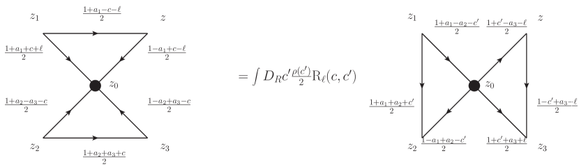
Figure 3: Diagrammatic representation of relation (33).

The expression for the kernel $\mathrm{R}_{\ell}(c,c^{\prime})$ can be obtained by using orthogonality relation (22)

$$\makebox[-10.00002pt]{}\int\mathrm{d}^{2}z_{0}\,\mathrm{d}^{2}z_{1}\,\mathrm{d}^{2}z_{2}\,W\left({-a_{1},-a_{2},-c^{\prime}\atop z_{1},z_{2},z_{3}^{\prime}}\right)W\left({a_{2},a_{3},c\atop z_{2},z_{3},z_{0}}\right)W\left({a_{1},c,\ell\atop z_{1},z_{0},z}\right)=\mathrm{R}_{\ell}(c,c^{\prime})W\left({c^{\prime},a_{3},\ell\atop z_{3}^{\prime},z_{3},z}\right).$$ (34)

The diagrammatic representation of this equality is given in Fig. 4. We have a diagram with three external vertices $z,z_{3},z_{3}^{\prime}$ and, due to the conformal invariance, it should coincide with the conformal triangle up to an overall coefficient $\mathrm{R}_{\ell}(c,c^{\prime})$. Vice versa, equations (33) and (34) can be derived from the completeness relations (29), (30).

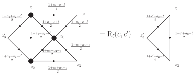
Figure 4: Diagrammatic representation of relation (34).

In the asymptotic regime when one of the coordinates $z,z_{3},z_{3}^{\prime}$ goes to infinity, e.g.

$$W\left({a_{1},a_{2},a_{3}\atop z_{1},z_{2},z_{3}}\right)\xrightarrow{z_{1}\to\infty}[z_{1}]^{-a_{1}}[z_{2}-z_{3}]^{-\frac{1-a_{1}+a_{2}-a_{3}}{2}},$$

we can reduce this three-point diagram to the two-point one. So, for $z_{3}\to\infty$ we obtain

$$\int\frac{\mathrm{d}^{2}z_{0}\,\mathrm{d}^{2}z_{1}\,\mathrm{d}^{2}z_{2}}{[z_{0}-z_{2}]^{\frac{1+a_{2}-a_{3}-c}{2}}}\,\overline{W\left({a_{1},a_{2},c^{\prime}\atop z_{1},z_{2},z_{3}^{\prime}}\right)}W\left({a_{1},c,\ell\atop z_{1},z_{0},z}\right)=\frac{\mathrm{R}_{\ell}(c,c^{\prime})}{[z-z_{3}^{\prime}]^{\frac{1+c^{\prime}-a_{3}-\ell}{2}}}.$$ (35)

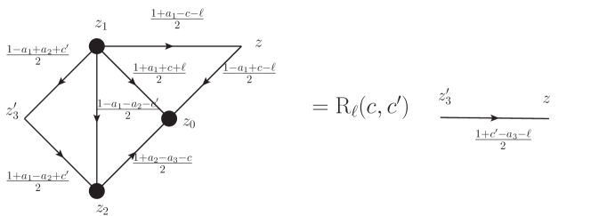
Figure 5: Diagrammatic representation of relation (35).

For $z_{3}^{\prime}\to\infty$, we have

$$\int\frac{\mathrm{d}^{2}z_{0}\,\mathrm{d}^{2}z_{1}\,\mathrm{d}^{2}z_{2}}{[z_{2}-z_{1}]^{\frac{1-a_{1}-a_{2}-c^{\prime}}{2}}}\,W\left({a_{2},a_{3},c\atop z_{2},z_{3},z_{0}}\right)W\left({a_{1},c,\ell\atop z_{1},z_{0},z}\right)=\frac{\mathrm{R}_{\ell}(c,c^{\prime})}{[z_{3}-z]^{\frac{1-c^{\prime}+a_{3}-\ell}{2}}},$$ (36)

Figure 6: Diagrammatic representation of relation (36).

,

and for $z\to\infty$

$$\int\frac{\mathrm{d}^{2}z_{0}\,\mathrm{d}^{2}z_{1}\,\mathrm{d}^{2}z_{2}}{[z_{0}-z_{1}]^{\frac{1+a_{1}+c+\ell}{2}}}\,\overline{W\left({a_{1},a_{2},c^{\prime}\atop z_{1},z_{2},z_{3}^{\prime}}\right)}W\left({a_{2},a_{3},c\atop z_{2},z_{3},z_{0}}\right)=\frac{\mathrm{R}_{\ell}(c,c^{\prime})}{[z_{3}-z_{3}^{\prime}]^{\frac{1+c^{\prime}+a_{3}+\ell}{2}}}.$$ (37)

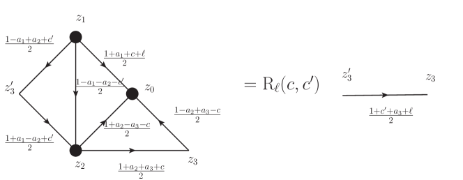
Figure 7: Diagrammatic representation of relation (37).

These relations are depicted in Figs. 5–7, where the limits diagrammatically correspond to the removal of two lines with the ends in the considered external vertex. Resulting two-point diagrams are fixed again by the conformal invariance to be given by a free propagator up an overall coefficient $\mathrm{R}_{\ell}(c,c^{\prime})$, which we call the value of the Feynman diagram of interest.

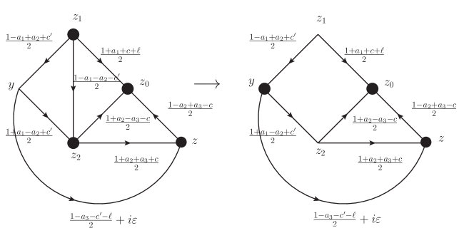
Figure 8: The parent diagram and the transition to an equivalent diagram.

All these three diagrams give identical evaluations, i.e. they represent symmetries of the corresponding function $\mathrm{R}_{\ell}(c,c^{\prime})$ as a function of its parameters. The origin of such a symmetry was discovered in [12]. Let us consider for example the diagram in Fig. 7. It belongs to the family of diagrams generated by the parent diagram shown on the left-hand side of Fig. 8. Namely, it emerges from it after removing the line with the index $i\varepsilon+(1-a_{3}-c^{\prime}-\ell)/2$, $\varepsilon\in\mathbb{R}$. The parent diagram has four integration vertices and one external vertex and it equals to

$$\mathrm{R}_{\ell}(c,c^{\prime})\int\mathrm{d}^{2}z\frac{1}{[z-y]^{\frac{1+c^{\prime}+a_{3}+\ell}{2}}}\frac{1}{[z-y]^{i\varepsilon+\frac{1-a_{3}-c^{\prime}-\ell}{2}}}=\mathrm{R}_{\ell}(c,c^{\prime})2\pi^{2}\delta(\varepsilon).$$ (38)

The main observation of [12] is that all diagrams obtained from such parent vacuum diagrams by removing one arbitrary line have the same value. We have shown in Fig. 8 the transition to one of the possible equivalent diagrams by removing the line with the index $(1-a_{1}-a_{2}-c^{\prime})/2$. The resulting diagram contains only three integration vertices and has the value

$$\mathrm{R}_{\ell}(c,c^{\prime})[z_{1}-z_{2}]^{-\frac{1+a_{1}+a_{2}+c^{\prime}}{2}-i\varepsilon}.$$

If we multiply this expression by the removed line propagator $[z_{1}-z_{2}]^{\frac{a_{1}+a_{2}+c^{\prime}-1}{2}}$ and integrate over $z_{1}$, we get again relation (38). Now we set in the right-hand side diagram in Fig. 8 $z_{1}=1,\,z_{2}=0$. As a result, the propagator part disappears. Since $\mathrm{R}_{\ell}(c,c^{\prime})$ does not depend on $\varepsilon$, we can take the limit $\varepsilon\to 0$ in the propagator connecting vertices $z$ and $y$. This yields an exact integral representation for $\mathrm{R}_{\ell}(c,c^{\prime})$:

$$\mathrm{R}_{\ell}(c,c^{\prime})=\int\mathrm{d}^{2}z\,\Phi_{2}(a_{1},a_{2},a_{3}|\ell,c,z)\overline{\Phi_{1}(a_{1},a_{2},a_{3}|\ell,c^{\prime},z)},$$ (39)

where

$$\overline{\Phi_{1}(a_{1},a_{2},a_{3}|\ell,c^{\prime},z)}=\int\frac{\mathrm{d}^{2}y}{[y-1]^{\frac{1-a_{1}+a_{2}+c^{\prime}}{2}}[-y]^{\frac{1+a_{1}-a_{2}+c^{\prime}}{2}}[z-y]^{\frac{1-a_{3}-\ell+c^{\prime}}{2}}},$$ (40)

$$\makebox[-20.00003pt]{}\Phi_{2}(a_{1},a_{2},a_{3}|\ell,c,z)=\frac{1}{[z]^{\frac{1+a_{2}+a_{3}+c}{2}}}\int\frac{\mathrm{d}^{2}z_{0}}{[z_{0}-1]^{\frac{1+a_{1}+\ell+c}{2}}[-z_{0}]^{\frac{1+a_{2}-a_{3}-c}{2}}[z_{1}-z]^{\frac{1-a_{2}+a_{3}-c}{2}}}.$$ (41)

In [15] Ismagilov has found the following representation for the same function

$$\mathrm{R}_{\ell}(c,c^{\prime})=\int\mathrm{d}^{2}z\,\Psi_{2}(a_{1},a_{2},a_{3}|\ell,c,z)\overline{\Psi_{1}(a_{1},a_{2},a_{3}|\ell,c^{\prime},z)},$$ (42)

where

$$\overline{\Psi_{1}(a_{1},a_{2},a_{3}|\ell,c^{\prime},z)}=\int\frac{\mathrm{d}^{2}y}{[1-y]^{\frac{1-\ell-c^{\prime}-a_{3}}{2}}[y]^{\frac{1+\ell-c^{\prime}+a_{3}}{2}}[z-y]^{\frac{1-a_{1}+a_{2}+c^{\prime}}{2}}},$$

$$\Psi_{2}(a_{1},a_{2},a_{3}|\ell,c,z)=\frac{1}{[z]^{\frac{1+a_{1}-\ell+c}{2}}}\int\frac{\mathrm{d}^{2}z_{0}}{[1-z_{0}]^{\frac{1+a_{1}+\ell+c}{2}}[z_{0}]^{\frac{1+a_{2}-a_{3}-c}{2}}[z-z_{0}]^{\frac{1-a_{2}+a_{3}-c}{2}}}.$$

We see that this expression has the same structure as our result, but indices of some propagators are different (sign differences in the arguments of $[1-y],[y],[1-z_{0}],[z_{0}]$ are inessential due to the constraints on the parity of integers $m_{j},m_{c},m_{c^{\prime}},m_{\ell}$). However, there is a symmetry transformation relating two expressions. The corresponding chain of transformations of diagrams is shown in Fig. 9. In its right-upper corner we give a more compact form of our diagram in Fig. 8. Then we use the chain integration rule and the star-triangle relation from Fig. 12. After that we arrive to the diagram in the right-lower corner in Fig. 9. Writing the corresponding integral representation one can see that it coincides with Ismagilov’s expression (42) after the replacement of his parameter $c^{\prime}$ by $-c^{\prime}$. So, our results almost coincide. This change $c^{\prime}\to-c^{\prime}$ corresponds to the replacement of the representation $\mathrm{T}_{c}$ in the first decomposition (31) by the equivalent representation $\mathrm{T}_{-c}$. Since this is a nontrivial action, it is necessary to understand the source of such a difference of our result with the one in [15].

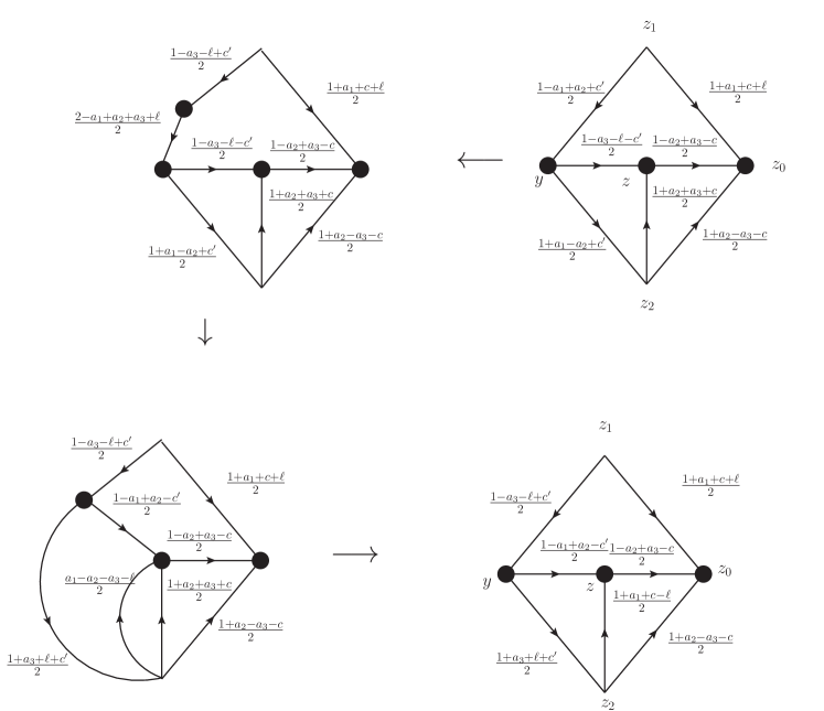
Figure 9: Transformation of the diagram.

5 Mellin-Barnes representation

In this section we derive a Mellin-Barnes type representation for the Racah coefficients described in the previous section. Let us fix $s=(n+i\nu)/2$, $\bar{s}=(-n+i\nu)/2$. There is a well-known representation for the two-dimensional delta function

$$\int Ds\left[\frac{x}{y}\right]^{s}\,=(2\pi)^{2}\,[x]\,\delta^{2}(x-y),\quad\int Ds:=\sum_{n\in\mathbb{Z}}\int_{\nu\in\mathbb{R}}d\nu.$$ (43)

Take a real variable $\varepsilon=\bar{\varepsilon}>0$, which will serve as a regularization parameter for infrared divergences. Then, with the help of formula (43) we can write

$$\frac{|y|^{2\varepsilon}}{[z-y]^{\alpha}}=\int d^{2}x\frac{|x|^{2\varepsilon}}{[z-x]^{\alpha}}\,\delta^{2}(x-y)=\frac{1}{(2\pi)^{2}}\int Ds\int d^{2}x\frac{1}{[z-x]^{\alpha}[x]^{1-s-\varepsilon}}\,\frac{1}{[y]^{s}}$$

$$\makebox[60.00009pt]{}=\frac{\pi a(\alpha)}{(2\pi)^{2}}\int Ds\,\frac{a(1-s-\varepsilon,1+s+\varepsilon-\alpha)}{[-z]^{\alpha-s-\varepsilon}[y]^{s}},$$

where we used the chain integration rule (50). Denote $\alpha=(n_{\alpha}+i\nu_{\alpha})/2$, $\bar{\alpha}=(-n_{\alpha}+i\nu_{\alpha})/2$, $n_{\alpha}\in\hbox{\bbd Z},\,\nu_{\alpha}\in\hbox{\bbd R}$. Poles of the integrand lie on the vertical half-lines at the points

$$\nu=i(-n+2\varepsilon+2\hbox{\bbd Z}_{\geq 0}),\quad\nu_{\alpha}+i(n-n_{\alpha}+2\varepsilon-2\hbox{\bbd Z}_{\geq 0}).$$

It is clearly seen that for $0<\varepsilon<1/2$ there are no singularities lying on the integration contour Im$(\nu)=0$ for all admissible values of $n\in\hbox{\bbd Z}$. Therefore we can change the integration contour to any contour lying in the strip $\text{Im}(\nu)\in]0,-1[$. After that we can take the limit $\varepsilon\to 0$ and come to the following Mellin-Barnes type representation of the propagator with an arbitrary index $\alpha$,

$$\frac{1}{[z-y]^{\alpha}}=\frac{1}{4\pi a(1-\alpha)}\sum_{n\in\mathbb{Z}}\int_{L}d\nu\,\frac{a(1-s,1+s-\alpha)}{[z]^{\alpha-s}[-y]^{s}},$$ (44)

where $L$ can be any contour lying in the strip $\text{Im}(\nu)\in]0,-1[$.

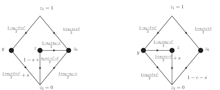
Figure 10: Mellin-Barnes representation diagrams.

Now we apply this formula to the line connecting the points $y$ and $z$ in the last diagram of Fig. 9. This yields an “integral” over the variable $s$ of the diagram given on the left-hand side of Fig. 10. However, the latter diagram can be calculated explicitly with the help of the chain rule (50). Omitting the details of computation, we obtain the following final Mellin-Barnes type representation for the $6j$-symbols

$$\mathrm{R}_{\ell}(c,c^{\prime})=(-1)^{c^{\prime}-\bar{c}^{\prime}}\,\frac{\pi^{2}}{4}\frac{a\left(\frac{1-a_{3}-\ell+c^{\prime}}{2},\frac{1+a_{1}+c+\ell}{2}\right)}{a\left(\frac{1+a_{1}-a_{2}+c^{\prime}}{2},\frac{1+a_{2}-a_{3}+c}{2}\right)}$$

$$\makebox[20.00003pt]{}\times\sum_{n\in\mathbb{Z}}\int_{L}d\nu\,\frac{a\left(\frac{1+a_{1}-a_{2}+c^{\prime}}{2}+s,\frac{1-a_{1}-a_{2}+c^{\prime}}{2}+s,\frac{1+a_{3}+\ell+c^{\prime}}{2}+s,\frac{1-a_{3}+\ell+c^{\prime}}{2}+s\right)}{a\left(s,c^{\prime}+s,\frac{c^{\prime}+\ell-a_{2}-c}{2}+s,\frac{c+c^{\prime}+\ell-a_{2}}{2}+s\right)}.$$ (45)

One can check that the integrands in (45) and in the $S$-function entering the Mellin-Barnes representation given in Theorem 2 of [16] coincide after shifting the variable $s\to s+(a_{2}-a_{1}-c^{\prime})/2$ (i.e. appropriate shifts of the summation variable $n$ and integration variable $\nu$) and denoting $z=i\nu/2$. However, the prefactor in front of the $S$-function in [16] misses the numerical multiplier $\pi^{2}/2i$ and differs from ours by the replacement $c^{\prime}\to-c^{\prime}$, as before.

Equivalently, it is possible to apply formula (44) to the line connecting $z$ and $z_{0}$ in the last diagram of Fig. 9. In this way we come to the right-hand side diagram in Fig. 10 which can be calculated again by using the rule (50). This yields the second Mellin-Barnes type representation of interest

$$\mathrm{R}_{\ell}(c,c^{\prime})=(-1)^{c^{\prime}-\bar{c}^{\prime}}\frac{\pi^{2}}{4}\,\frac{a\left(\frac{1-a_{3}-\ell+c^{\prime}}{2},\frac{1+a_{1}+c+\ell}{2}\right)}{a\left(\frac{1+a_{1}-a_{2}+c^{\prime}}{2},\frac{1+a_{2}-a_{3}+c}{2}\right)}$$

$$\makebox[20.00003pt]{}\times\sum_{n\in\mathbb{Z}}\int_{L}d\nu\,\frac{a\left(\frac{1+a_{2}-a_{3}+c}{2}+s,\frac{1+a_{1}-\ell+c}{2}+s,\frac{1+a_{2}+a_{3}+c}{2}+s,\frac{1-a_{1}-\ell+c}{2}+s\right)}{a\left(s,c+s,\frac{a_{2}+c-\ell-c^{\prime}}{2}+s,\frac{a_{2}+c-\ell+c^{\prime}}{2}+s\right)}.$$ (46)

One can see that this expression is obtained from (45) simply by the shift of the variable $s\to s+(a_{2}-\ell-c^{\prime}+c)/2$.

6 Conclusion

In this work we have computed $6j$-symbols for the unitary principal series representaion of the group $\mathrm{SL}(2,\mathbb{C})$, which are described by formulas (39)-(41). They coincide with the Racah coefficients obtained by Ismagilov [15] up to the replacement in his expression for them the representation parameter $c^{\prime}$ by $-c^{\prime}$. Note, however, that our result is slightly more general than in [15], since we do not assume that the integer representation parameters $m_{j}$ are even.

As shown in [15], the Mellin-Barnes representation for $\mathrm{R}_{\ell}(c,c^{\prime})$ can be rewritten in an equivalent form as a sum of the products of two ${}_{4}F_{3}$ hypergeometric series with different arguments. We do not present the corresponding cumbersome expressions here.

We expect that the derived function $\mathrm{R}_{\ell}(c,c^{\prime})$ describes Boltzmann weights of an IRF type integrable two-dimensional statistical mechanics model and, so, solves the corresponding Yang-Baxter equation. On the basis of the described approach it is possible to build more general $6j$-symbols related to the very-well poised ${}_{9}F_{8}$-series. In principle, following the results of [7], it is possible to establish a relation to elliptic $6j$-symbols described by the $V$-function presented in [24] (an elliptic extension of the Euler-Gauss hypergeometric function), which is a subject for a separate consideration.

Acknowledgements. This work is supported by the Russian Science Foundation (project no. 14-11-00598).

7 Appendix

In the diagram technique we use, the kernels of operators are represented in the form of two-dimensional Feynman integrals. The propagator, which is shown by the arrow directed from $w$ to $z$ and index $\alpha$ attached to it as in Fig. 11, is given by the following expression

$$\frac{1}{[z-w]^{\alpha}}\equiv\frac{1}{(z-w)^{\alpha}(\bar{z}-\bar{w})^{\bar{\alpha}}}=\frac{(\bar{z}-\bar{w})^{\alpha-\bar{\alpha}}}{|z-w|^{2\alpha}}=\frac{(-1)^{\alpha-\bar{\alpha}}}{[w-z]^{\alpha}},$$ (47)

where $\alpha-\bar{\alpha}=n_{\alpha}$ is an integer. On the same figure we indicate the result of the flipping of the direction of the line.

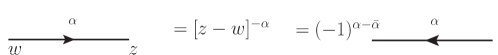
Figure 11: The propagator and a flip of the arrow.

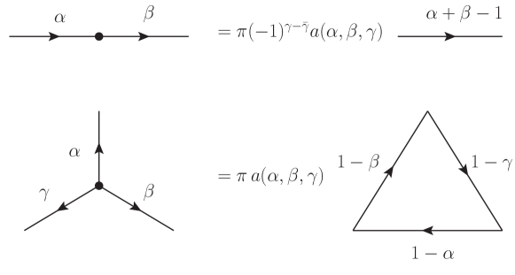
Figure 12: The chain and star-triangle relations, $\alpha+\beta+\gamma=2$.

After the Fourier transformation we obtain the propagator in the momentum representation

$$\int d^{2}z\frac{e^{i(pz+\bar{p}\bar{z})}}{[z]^{\alpha}}=\pi\,i^{\alpha-\bar{\alpha}}\,a(\alpha)\,\frac{1}{[p]^{1-\alpha}},$$ (48)

where

$$a(\alpha)=\frac{\Gamma(1-\bar{\alpha})}{\Gamma(\alpha)},\quad a(\bar{\alpha})=\frac{\Gamma(1-\alpha)}{\Gamma(\bar{\alpha})},\quad a(\alpha,\beta,\gamma,\ldots):=a(\alpha)a(\beta)a(\gamma)\ldots.$$ (49)

The function $a(\alpha)$ has the following properties

$$a(\alpha)a(1-\bar{\alpha})=1,\qquad\frac{a(1+\alpha)}{a(\alpha)}=-\frac{1}{\alpha\bar{\alpha}},$$

$$a(\alpha)a(1-\alpha)=(-1)^{\alpha-\bar{\alpha}},\qquad a(\alpha)=(-1)^{\alpha-\bar{\alpha}}a(\bar{\alpha}).$$

Our evaluations of Feynman diagrams are based on the following computation rules.

• Chain relation:

  $$\int d^{2}w\frac{1}{[z_{1}-w]^{\alpha}[w-z_{2}]^{\beta}}=\frac{\pi a(\alpha,\beta,\gamma)}{[z_{2}-z_{1}]^{\alpha+\beta-1}},$$ (50)

  where $\gamma=2-\alpha-\beta,\ \bar{\gamma}=2-\bar{\alpha}-\bar{\beta}$.

• Star-triangle relation:

  $$\int d^{2}w\frac{1}{[z_{1}-w]^{\alpha}[z_{2}-w]^{\beta}[z_{3}-w]^{\gamma}}=\frac{\pi a(\alpha,\beta,\gamma)}{[z_{2}-z_{1}]^{1-\gamma}[z_{1}-z_{3}]^{1-\beta}[z_{3}-z_{2}]^{1-\alpha}},$$ (51)

  where $\alpha+\beta+\gamma=2$ and $\bar{\alpha}+\bar{\beta}+\bar{\gamma}=2$.

These identities are depicted in the diagrammatic form in Fig. 12, where the blob means the integration over the vertex coordinate.

- [1] G. E. Andrews, R. Askey, and R. Roy, Special Functions, Encyclopedia of Math. Appl. 71, Cambridge Univ. Press, Cambridge, 1999.
- [2] A. A. Belavin, A. M. Polyakov, and A. B. Zamolodchikov, Infinite conformal symmetry in two-dimensional quantum field theory, Nucl. Phys. B 241:2 (1984), 333–380.
- [3] D. Chicherin, S. E. Derkachov, and V. P. Spiridonov, From principal series to finite-dimensional solutions of the Yang-Baxter equation, SIGMA 12 (2016), 028.
- [4] S. E. Derkachov and L. D. Faddeev, -symbol for the modular double of revisited, J. Phys.: Conf. Ser. 532 (2014), 012005.
- [5] S. E. Derkachov and A. N. Manashov, General solution of the Yang-Baxter equation with the symmetry group , Algebra i Analiz 21 (4) (2009), 1–94 (St. Petersburg Math. J. 21 (2010), 513–577).
- [6] S. E. Derkachov and A. N. Manashov, Spin chains and Gustafson’s integrals, J. Phys. A: Math. Theor. 50 (2017), 294006.
- [7] S. E. Derkachov and A. N. Manashov, and P. A. Valinevich, Gustafson integrals for spin magnet, J. Phys. A: Math. Theor. 50 (2017), 294007.
- [8] L. D. Faddeev, Modular double of a quantum group, Conf. Moshé Flato 1999, vol. I, Math. Phys. Stud. 21, Kluwer, Dordrecht, 2000, pp. 149–156.
- [9] L. D. Faddeev and G. P. Korchemsky, High-energy QCD as a completely integrable model, Phys. Lett. B 342 (1995), 311–322.
- [10] I. M. Gelfand, M. I. Graev, and N. Ya. Vilenkin, Generalized functions, Vol. 5, Academic Press, 1966.
- [11] I. M. Gelfand, M. A. Naimark, Unitary representations of the classical groups, Trudy Mat. Inst. Steklov 36 (1950), 3–288.
- [12] S. G. Gorishnii, A. P. Isaev, An approach to the calculation of many-loop massless Feynman integrals, Teor. Mat. Fiz. 62:3 (1985), 345–358 (Theor. Math. Phys. 62:3 (1985), 232–240).
- [13] W. Groenevelt, Wilson function transforms related to Racah coefficients, Acta Appl. Math. 91:2 (2006), 133–191.
- [14] L. Hadasz, M. Pawelkiewicz, and V. Schomerus, Self-dual Continuous Series of Representations for and , J. High Energy Phys. 1410 (2014), 091.
- [15] R. S. Ismagilov, On Racah operators, Funktsional. Anal. i Prilozhen. 40:3 (2006), 69–72 (Funct. Anal. Appl. 40:3 (2006), 222–224).
- [16] R. S. Ismagilov, Racah operators for principal series of representations of the group , Mat. Sbornik 198:3 (2007), 77–90 (Sb. Math. 198:3 (2007), 369–381).
- [17] L. N. Lipatov, The bare Pomeron in quantum chromodynamics Zh. Eksp. Teor. Fiz. 90 (1986), 1536–1552 (Sov. Phys. JETP 63 (1986), 904–912).
- [18] L. N. Lipatov, High-energy asymptotics of multicolor QCD and two-dimensional conformal field theories, Phys. Lett. B 309 (1993), 394–396.
- [19] L. N. Lipatov, High-energy asymptotics of multicolor QCD and exactly solvable lattice models, Pisma Zh. Eksp. Teor. Fiz. 59 (1994), 571–574 (JETP Lett. 59 (1994), 596–599).
- [20] M. A. Naimark, Decomposition of a tensor product of irreducible representations of the proper Lorentz group into irreducible representations, Tr. Mosk. Mat. Obs. 8 (1959), 121–153 (Am. Math. Soc. Transl., Ser. 2, Vol. 36 (1964), 101–229).
- [21] M. Pawelkiewicz, V. Schomerus, and P. Suchanek, The universal Racah-Wigner symbol for , J. High Energy Phys. 1404 (2014), 079.
- [22] B. Ponsot and J. Teschner, Clebsch-Gordan and Racah-Wigner coefficients for a continuous series of representations of , Commun. Math. Phys. 224 (2001), 613–655.
- [23] G. Racah, Theory of complex spectra. II, Phys. Rev. 62 (1942), 438–462.
- [24] V. P. Spiridonov, Essays on the theory of elliptic hypergeometric functions, Uspekhi Mat. Nauk 63, no. 3 (2008), 3–72 (Russian Math. Surveys 63 (3) (2008), 405–472).
- [25] D. A. Varshalovich, A. N. Moskalev, and V. K. Khersonskii, Quantum Theory of Angular Momentum, World Scientific, Singapore, 1988.