Conditionally conjugate mean–field variational Bayes for logistic models

Abstract

Variational Bayes (vb) is a common strategy for approximate Bayesian inference, but simple methods are only available for specific classes of models including, in particular, representations having conditionally conjugate constructions within an exponential family. Models with logit components are an apparently notable exception to this class, due to the absence of conjugacy between the logistic likelihood and the Gaussian priors for the coefficients in the linear predictor. To facilitate approximate inference within this widely used class of models, Jaakkola and Jordan (2000) proposed a simple variational approach which relies on a family of tangent quadratic lower bounds of logistic log-likelihoods, thus restoring conjugacy between these approximate bounds and the Gaussian priors. This strategy is still implemented successfully, but less attempts have been made to formally understand the reasons underlying its excellent performance. To cover this key gap, we provide a formal connection between the above bound and a recent Pólya-gamma data augmentation for logistic regression. Such a result places the computational methods associated with the aforementioned bounds within the framework of variational inference for conditionally conjugate exponential family models, thereby allowing recent advances for this class to be inherited also by the methods relying on Jaakkola and Jordan (2000).

and

Department of Decision Sciences and Bocconi Institute for Data Science and Analytics, Bocconi University, Via Roentgen 1, Milan, Italy .

1 Introduction

The increasing availability of massive and high–dimensional datasets has motivated a wide interest in strategies for Bayesian learning of posterior distributions, beyond classical mcmc methods (e.g. Gelfand and Smith, 1990). Indeed, sampling algorithms can face severe computational bottlenecks in complex statistical models, thus motivating alternative solutions based on scalable and efficient optimization of approximate posterior distributions. Notable methods within this class are the Laplace approximation (e.g. Bishop, 2006, Ch. 4.4), variational Bayes (e.g. Bishop, 2006, Ch. 10.1) and expectation propagation (e.g. Bishop, 2006, Ch. 10.7), with variational inference providing a standard choice in several fields, as discussed in recent reviews by Blei, Kucukelbir and McAuliffe (2017) and Ormerod and Wand (2010). Refer also to Jordan et al. (1999) for a seminal introduction of variational inference from a statistical perspective.

Adapting the notation in Blei, Kucukelbir and McAuliffe (2017), vb aims at obtaining a tractable approximation $q^{*}({\bm{\theta}})$ for the posterior distribution $p({\bm{\theta}}\mid{\bf y})$ of the random coefficients ${\bm{\theta}}=(\theta_{1},\ldots,\theta_{m})^{\intercal}$, in the model having joint density $p({\bf y},{\bm{\theta}})=p({\bf y}\mid{\bm{\theta}})p({\bm{\theta}})$ for ${\bm{\theta}}$ and the observed data ${\bf y}=(y_{1},\ldots,y_{n})^{\intercal}$, with $p({\bm{\theta}})$ denoting the prior distribution for ${\bm{\theta}}$. This optimization problem is formally addressed by minimizing the Kullback–Leibler (kl) divergence (Kullback and Leibler, 1951)

$$\textsc{kl}[q({\bm{\theta}})\mid\mid p({\bm{\theta}}\mid{\bf y})]=\int_{{\bm{\Theta}}}q({\bm{\theta}})\log\frac{q({\bm{\theta}})}{p({\bm{\theta}}\mid{\bf y})}\mbox{d}{\bm{\theta}}=\int_{{\bm{\Theta}}}q({\bm{\theta}})\log\frac{q({\bm{\theta}})p({\bf y})}{p({\bf y},{\bm{\theta}})}\mbox{d}{\bm{\theta}},$$ (1)

with respect to $q({\bm{\theta}})\in\mathcal{Q}$, where $\mathcal{Q}$ denotes a tractable, yet sufficiently flexible, class of approximating distributions. As is clear from (1), the calculation of the kl divergence between $q({\bm{\theta}})$ and the posterior $p({\bm{\theta}}\mid{\bf y})$ requires the evaluation of the normalizing constant $p({\bf y})$, whose intractability is actually the main reason motivating approximate Bayesian methods. Due to this, the above minimization problem is commonly translated into the maximization of the evidence lower bound (elbo) function

$$\textsc{elbo}[q({\bm{\theta}})]=\int_{{\bm{\Theta}}}q({\bm{\theta}})\log\frac{p({\bf y},{\bm{\theta}})}{q({\bm{\theta}})}\mbox{d}{\bm{\theta}}=-\textsc{kl}[q({\bm{\theta}})\mid\mid p({\bm{\theta}}\mid{\bf y})]+\log p({\bf y}),$$ (2)

which does not require the evaluation of $p({\bf y})$. In fact, since $\log p({\bf y})$ does not depend on ${\bm{\theta}}$, maximizing (2) is equivalent to minimizing (1). Re–writing (2) as $\log p({\bf y})=\textsc{elbo}[q({\bm{\theta}})]+\textsc{kl}[q({\bm{\theta}})\mid\mid p({\bm{\theta}}\mid{\bf y})]$ it can be additionally noticed that the elbo provides a lower bound of $\log p({\bf y})$ for any $q({\bm{\theta}})$, since the Kullback–Leibler divergence is always non–negative (Kullback and Leibler, 1951).

The above set–up defines the general rationale underlying vb but, as is clear from (2), the practical feasibility of the variational optimization requires a tractable form for the joint density $p({\bf y},{\bm{\theta}})$ along with a simple, yet flexible, variational family $\mathcal{Q}$. This is the case of mean–field vb for conditionally conjugate exponential family models with global and local variables (Wang and Titterington, 2004; Bishop, 2006; Hoffman et al., 2013; Blei, Kucukelbir and McAuliffe, 2017). Recalling Hoffman et al. (2013), these methods focus on obtaining a mean–field approximation

$$\begin{split}q^{*}({\bm{\theta}})=q^{*}({\bm{\beta}},{\bf z})=q^{*}({\bm{\beta}})\prod\nolimits_{i=1}^{n}q^{*}(z_{i})=\mbox{argmin}\{\textsc{kl}[q({\bm{\beta}})\prod\nolimits_{i=1}^{n}q(z_{i})\mid\mid p({\bm{\beta}},{\bf z}\mid{\bf y})]\},&\\ =\mbox{argmax}\{\textsc{elbo}[q({\bm{\beta}})\prod\nolimits_{i=1}^{n}q(z_{i})]\}\qquad\qquad\ &\end{split}$$ (3)

for the posterior distribution $p({\bm{\beta}},{\bf z}\mid{\bf y})$ of the global coefficients ${\bm{\beta}}=(\beta_{1},\ldots,\beta_{p})^{\intercal}$ and the local variables ${\bf z}=(z_{1},\ldots,z_{n})^{\intercal}$ in the statistical model having joint density

$$p({\bf y},{\bm{\beta}},{\bf z})=p({\bm{\beta}})\prod\nolimits_{i=1}^{n}p(z_{i}\mid{\bm{\beta}})p(y_{i}\mid z_{i},{\bm{\beta}})=p({\bm{\beta}})\prod\nolimits_{i=1}^{n}p(y_{i},z_{i}\mid{\bm{\beta}}),$$ (4)

with $p(y_{i},z_{i}\mid{\bm{\beta}})$ from an exponential family and $p({\bm{\beta}})$ being a conjugate prior for this density. The latent quantities ${\bf z}$—when present—typically denote random effects or unit–specific augmented data within some hierarchical formulation, such as in mixture models.

Although the above assumptions appear restrictive, the factorization of $q({\bm{\beta}},{\bf z})$—characterizing the mean–field variational family—provides a flexible class in several applications and allows direct implementation of simple coordinate ascent variational inference (cavi) routines (Bishop, 2006, Ch. 10.1.1) which sequentially maximize the elbo in (LABEL:eq31) with respect to each factor in $q({\bm{\beta}},{\bf z})=q({\bm{\beta}})\prod_{i=1}^{n}q(z_{i})$—fixing the others at their most recent update. Instead, the exponential family and conjugacy assumptions further simply calculations by providing approximating densities $q^{*}({\bm{\beta}})$ and $q^{*}(z_{i})$, $i=1,\ldots,n$ from tractable classes of random variables. These advantages have also motivated recent computational improvements (Hoffman et al., 2013) and theoretical studies (Wang and Titterington, 2004). We refer to Hoffman et al. (2013) and Blei, Kucukelbir and McAuliffe (2017) for details on the methods related to the general formulation in (LABEL:eq31)–(4), and focus here on models having logistic likelihoods as building–blocks. Indeed, although the conjugacy and exponential family assumptions are common to a variety of machine learning representations (e.g. Blei, Ng and Jordan, 2003; Airoldi et al., 2008; Hoffman et al., 2013), classical Bayesian logistic regression models of the form

$$p(y_{i}\mid{\bm{\beta}})=\frac{[\exp({\bf x}_{i}^{\intercal}{\bm{\beta}})]^{y_{i}}}{1+\exp({\bf x}_{i}^{\intercal}{\bm{\beta}})},\ \ y_{i}\in\{0,1\},\ i=1,\ldots,n,\quad\mbox{with }{\bm{\beta}}\sim\mbox{N}_{p}({\bm{\mu}}_{0},{\bm{\Sigma}}_{0}),$$ (5)

do not enjoy direct conjugacy between the likelihood for the binary response data and the Gaussian prior for the coefficients in the linear predictor (e.g. Wang and Blei, 2013). This apparently notable exception to conditionally conjugate exponential family models also holds, as a direct consequence, for a wide set of formulations which incorporate Bayesian logistic regressions at some layer of the hierarchical specification. Some relevant examples are classification via Gaussian processes (Rasmussen and Williams, 2006), supervised nonparametric clustering (Ren et al., 2011) and hierarchical mixture of experts (Bishop and Svensén, 2003).

Initialize $\xi_{1}^{(0)},\ldots,\xi^{(0)}_{n}$.

for $t=1$ until convergence of (7) do

        E–step. Update $q^{(t)}({\bm{\beta}})=\bar{p}^{(t-1)}({\bm{\beta}}\mid{\bf y})\propto p({\bm{\beta}})\prod_{i=1}^{n}\bar{p}^{(t-1)}(y_{i}\mid{\bm{\beta}})$ to obtain a $\mbox{N}_{p}({\bm{\mu}}^{(t)}{,}{\bm{\Sigma}}^{(t)})$ density with

$${\bm{\Sigma}}^{(t)}=({\bm{\Sigma}}_{0}^{-1}+{\bf X}^{\intercal}\bar{{\bf Z}}^{(t-1)}{\bf X})^{-1},\qquad{\bm{\mu}}^{(t)}={\bm{\Sigma}}^{(t)}[{\bf X}^{\intercal}({\bf y}-0.5{\cdot}{\bf 1}_{n})+{\bm{\Sigma}}_{0}^{-1}{\bm{\mu}}_{0}],$$

where ${\bf 1}_{n}=(1,\ldots,1)^{\intercal}$ and $\bar{{\bf Z}}^{(t-1)}=\mbox{diag}\{0.5[\xi_{1}^{(t-1)}]^{-1}\mbox{tanh}(0.5\xi^{(t-1)}_{1}),\ldots,0.5[\xi_{n}^{(t-1)}]^{-1}\mbox{tanh}(0.5\xi^{(t-1)}_{n})\}$. Note that the quadratic form of (6), restores conjugacy between the Gaussian prior for ${\bm{\beta}}$ and the approximated likelihood. To clarify this result, note that, for every $\xi_{i}$, $\bar{p}(y_{i}\mid{\bm{\beta}})$ is proportional to the kernel of a normal with mean ${\bf x}_{i}^{\intercal}{\bm{\beta}}$ and variance $2\xi_{i}\mbox{{tanh}}(0.5\xi_{i})^{-1}$ for transformed data $2\xi_{i}\mbox{{tanh}}(0.5\xi_{i})^{-1}(y_{i}-0.5)$.

        M–step. Compute ${\bm{\xi}}^{(t)}=\mbox{argmax}_{{\bm{\xi}}}\int_{\Re^{p}}{q}^{(t)}({\bm{\beta}})\log\bar{p}({\bf y},{\bm{\beta}})\mbox{d}{\bm{\beta}}$ to obtain the solutions

$$\xi^{(t)}_{i}=\{\mathbb{E}_{{q}^{(t)}({\bm{\beta}})}[({\bf x}_{i}^{\intercal}{\bm{\beta}})^{2}]\}^{\frac{1}{2}}=[{\bf x}^{\intercal}_{i}{\bm{\Sigma}}^{(t)}{\bf x}_{i}{+}({\bf x}_{i}^{\intercal}{\bm{\mu}}^{(t)})^{2}]^{\frac{1}{2}},\quad\mbox{for every }i=1,\ldots,n.$$

Note that $\int_{\Re^{p}}{q}^{(t)}({\bm{\beta}})\log\bar{p}({\bf y},{\bm{\beta}})\mbox{d}{\bm{\beta}}=\mbox{const}+\sum_{i=1}^{n}\int_{\Re^{p}}{q}^{(t)}({\bm{\beta}})\log\bar{p}(y_{i}\mid{\bm{\beta}})\mbox{d}{\bm{\beta}}$. Hence, it is possible to maximize the expected log-likelihood associated with every $y_{i}$ separately, as a function of each $\xi_{i}$, for $i=1,\ldots,n$. This result leads to the above solution.

Output at the end of the algorithm: ${\bm{\xi}}^{*}$ and, as a byproduct, the approximate posterior ${q}^{*}({\bm{\beta}})=\bar{p}^{*}({\bm{\beta}}\mid{\bf y})$.

Algorithm 1 em algorithm for approximate Bayesian inference by Jaakkola and Jordan (2000).

To allow tractable vb for non–conjugate models, several alternatives beyond conjugate mean–field vb have been proposed (see e.g. Jaakkola and Jordan, 2000; Braun and McAuliffe, 2010; Wand et al., 2011; Wang and Blei, 2013). Within the context of logistic regression, Jaakkola and Jordan (2000) developed a seminal vb algorithm which relies on the quadratic lower bound

$$\qquad\log\bar{p}(y_{i}\mid{\bm{\beta}})=(y_{i}-0.5){\bf x}_{i}^{\intercal}{\bm{\beta}}-0.5\xi_{i}-0.25\xi_{i}^{-1}\mbox{{tanh}}(0.5\xi_{i})[({\bf x}_{i}^{\intercal}{\bm{\beta}})^{2}-\xi_{i}^{2}]-\log[1+\exp(-\xi_{i})],$$ (6)

for the log-likelihood $\log p(y_{i}\mid{\bm{\beta}})=y_{i}({\bf x}_{i}^{\intercal}{\bm{\beta}})-\log[1+\exp({\bf x}_{i}^{\intercal}{\bm{\beta}})]\geq\log\bar{p}(y_{i}\mid{\bm{\beta}})$ of every $y_{i}$ from a logistic regression. In (6), the vector ${\bf x}_{i}=(x_{i1},\ldots,x_{ip})^{\intercal}$ comprises the covariates measured for unit $i$, whereas ${\bm{\beta}}=(\beta_{1},\ldots,\beta_{p})^{\intercal}$ are the associated coefficients. The vector ${\bm{\xi}}=(\xi_{1},\ldots,\xi_{n})^{\intercal}$ denotes instead unit–specific variational parameters defining the location where $\log\bar{p}(y_{i}\mid{\bm{\beta}})$ is tangent to $\log p(y_{i}\mid{\bm{\beta}})$. In fact, $\log\bar{p}(y_{i}\mid{\bm{\beta}})=\log p(y_{i}\mid{\bm{\beta}})$ when $\xi_{i}^{2}=({\bf x}_{i}^{\intercal}{\bm{\beta}})^{2}$. Leveraging equation (6), Jaakkola and Jordan (2000) proposed an expectation–maximization (em) algorithm (Dempster, Laird and Rubin, 1977) to approximate $p({\bm{\beta}}\mid{\bf y})$. At the generic iteration $t$, this routine alternates between an e–step in which the conditional distribution of the random coefficients ${\bm{\beta}}$ given the current ${\bm{\xi}}^{(t-1)}$ is updated to obtain ${q}^{(t)}({\bm{\beta}})$, and an m–step which calculates the expectation of the augmented approximate log-likelihood $\log\bar{p}({\bf y},{\bm{\beta}})=\log p({\bm{\beta}})+\sum_{i=1}^{n}\log\bar{p}(y_{i}\mid{\bm{\beta}})$ with respect to ${q}^{(t)}({\bm{\beta}})$ and maximizes it as a function of ${\bm{\xi}}$. Recalling the general presentation of em by Bishop (2006, Ch. 9.4) and Appendices A–B in Jaakkola and Jordan (2000), this strategy ultimately maximizes $\log\bar{p}({\bf y})=\log\int_{\Re^{p}}p({\bm{\beta}})\prod_{i=1}^{n}\bar{p}(y_{i}\mid{\bm{\beta}})\mbox{d}{\bm{\beta}}$ with respect to ${\bm{\xi}}$, by sequentially optimizing the lower bound

$$\int_{\Re^{p}}q({\bm{\beta}})\log\frac{p({\bm{\beta}})\prod_{i=1}^{n}\bar{p}(y_{i}\mid{\bm{\beta}})}{q({\bm{\beta}})}\mbox{d}{\bm{\beta}},$$ (7)

as a function of the unknown distribution $q({\bm{\beta}})$ and the fixed parameters ${\bm{\xi}}$, where $p({\bm{\beta}})$ is the density of the Gaussian prior for ${\bm{\beta}}$. Hence, as is clear from Algorithm 1, this em produces an optimal estimate ${\bm{\xi}}^{*}$ of ${\bm{\xi}}$ and, as a byproduct, also a distribution ${q}^{*}({\bm{\beta}})$, which is regarded as an approximate posterior in Jaakkola and Jordan (2000). Indeed, recalling the em structure, ${q}^{*}({\bm{\beta}})$ coincides with the conditional distribution $\bar{p}^{*}({\bm{\beta}}\mid{\bf y})$ obtained by updating the prior $p({\bm{\beta}})$ with the approximate likelihood $\prod_{i=1}^{n}\bar{p}^{*}(y_{i}\mid{\bm{\beta}})$ induced by (6) and evaluated at the optimal variational parameters $\xi^{*}_{1},\ldots,\xi^{*}_{n}$. However, although being successfully implemented in the machine learning and statistical literature (e.g. Bishop and Svensén, 2003; Rasmussen and Williams, 2006; Lee, Huang and Hu, 2010; Ren et al., 2011; Carbonetto and Stephens, 2012; Tang, Browne and McNicholas, 2015; Wand, 2017), it is not clear how the solution ${q}^{*}({\bm{\beta}})$ relates to the formal vb set–up in (1)–(2). Indeed, $\bar{p}^{*}({\bm{\beta}}\mid{\bf y})$ is not the posterior induced by a Bayesian logistic regression. This is due to the fact that each $p(y_{i}\mid{\bm{\beta}})$ in the kernel of $p({\bm{\beta}}\mid{\bf y})$ is replaced with the approximate likelihood $\bar{p}^{*}(y_{i}\mid{\bm{\beta}})$ evaluated at the optimal variational parameters maximizing $\log\bar{p}({\bf y})$. This last result, which is inherent to the em (Dempster, Laird and Rubin, 1977), suggests an heuristic intuition for why ${q}^{*}({\bm{\beta}})$ may still provide a reasonable approximation. Indeed, since $\log\bar{p}(y_{i}\mid{\bm{\beta}})\leq\log p(y_{i}\mid{\bm{\beta}})$ for every $\xi_{i}$ and $i=1,\ldots,n$, the same holds for $\log\bar{p}({\bf y})$ and $\log p({\bf y})$. Thus, since $\log p({\bf y})$ does not vary with ${\bm{\xi}}$, maximizing $\log\bar{p}({\bf y})$ with respect to ${\bm{\xi}}$ is expected to provide the tightest approximation of each $\log p(y_{i}\mid{\bm{\beta}})$ via the lower bound in (6) evaluated at the optimum $\xi^{*}_{i}$, for $i=1,\ldots,n$, thereby guaranteeing similar predictive densities $p({\bf y})$ and $\bar{p}^{*}({\bf y})$. Hence, in correspondence to ${\bm{\xi}}^{*}$, the minimization of $\textsc{kl}[q({\bm{\beta}})\mid\mid\bar{p}^{*}({\bm{\beta}}\mid{\bf y})]$ in the e–step, would hopefully provide a solution ${q}^{*}({\bm{\beta}})=\bar{p}^{*}({\bm{\beta}}\mid{\bf y})$ close to the true posterior $p({\bm{\beta}}\mid y)$.

Although the above discussion provides an intuition for the excellent performance of the methods proposed by Jaakkola and Jordan (2000), it shall be noticed that finding the tightest bound within a class of functions might not be sufficient if this class is not flexible enough. Indeed, the quadratic form of (6) might be restrictive for logistic log-likelihoods, and hence even the optimal approximation may fail to mimic $\log p(y_{i}\mid{\bm{\beta}})$. Moreover, according to (1), a formal vb set–up requires the minimization of a well–defined kl divergence between an exact posterior and an approximating density from a given variational family. Instead, Jaakkola and Jordan (2000) seem to minimize the divergence between an approximate posterior and a pre–specified density. If this were the case, then their methods could be only regarded as approximate solutions to formal vb. Indeed, although (6) has been recently studied (De Leeuw and Lange, 2009; Browne and McNicholas, 2015), this is currently the main view of the em in Algorithm 1 (e.g. Blei, Kucukelbir and McAuliffe, 2017; Wang and Blei, 2013; Bishop, 2006).

In Section 2 we prove that this is not true and that (6), although apparently supported by purely mathematical arguments, has indeed a clear probabilistic interpretation related to a recent Pólya-gamma data augmentation for logistic regression (Polson, Scott and Windle, 2013). In particular, let $q(z_{i})$ be the density of a Pólya-gamma $\textsc{pg}(1,\xi_{i})$, then (6) is a proper evidence lower bound associated with a vb approximation of the posterior for $z_{i}$ in the conditional model $p(y_{i},z_{i}\mid{\bm{\beta}})$ for data $y_{i}$ from (5) and the Pólya-gamma variable $(z_{i}\mid{\bm{\beta}})\sim\textsc{pg}(1,{\bf x}_{i}^{\intercal}{\bm{\beta}})$, with ${\bm{\beta}}$ kept fixed. Combining this result with the objective function in equation (7), allows us to formalize Algorithm 1 as a pure cavi which approximates the joint posterior of ${\bm{\beta}}$ and the augmented Pólya-gamma data $z_{1},\ldots,z_{n}$, under a mean–field variational approximation within a conditionally conjugate exponential family framework. These results are discussed in Section 3, and are further generalized to allow stochastic variational inference (Hoffman et al., 2013) in logistic models, thus covering an important computational gap. A final discussion can be found in Section 4. Codes and additional empirical assessments are available at https://github.com/tommasorigon/logisticVB. Although we focus on Bayesian inference, it shall be noticed that (6) motivates also an em for maximum likelihood estimation of ${\bm{\beta}}$ (Jaakkola and Jordan, 2000, Appendix C). We derive the optimality properties of this routine in the Appendix.

2 Conditionally conjugate variational representation

This section discusses the theoretical connection between equation (6) and a recent Pólya-gamma data augmentation for conditionally conjugate inference in Bayesian logistic regression (Polson, Scott and Windle, 2013), thus allowing us to recast the methods proposed by Jaakkola and Jordan (2000) within the wider framework of mean–field variational inference for conditionally conjugate exponential family models. We shall emphasize that, in a recent manuscript, Scott and Sun (2013) proposed an em for maximum a posteriori estimation of ${\bm{\beta}}$ in (5), discussing connections with the variational methods in Jaakkola and Jordan (2000). Their findings are however limited to computational differences and similarities among the two methods and the associated algorithms. We instead provide a fully probabilistic connection between the contribution by Jaakkola and Jordan (2000) and the one of Polson, Scott and Windle (2013), thus opening new avenues for advances in vb for logistic models.

To anticipate Lemma 1, note that the core contribution of Polson, Scott and Windle (2013) is in showing that $p(y_{i}\mid{\bm{\beta}})$ in model (5) can be expressed as a scale–mixture of Gaussians with respect to a Pólya-gamma density. This result facilitates the implementation of mcmc methods which update ${\bm{\beta}}$ and the Pólya-gamma augmented data ${\bf z}=(z_{1},\ldots,z_{n})^{\intercal}$ from conjugate full conditionals. In fact, the joint density $p({\bf y},{\bf z}\mid{\bm{\beta}})$ has a Gaussian kernel in ${\bm{\beta}}$, thus restoring Gaussian–Gaussian conjugacy in the full conditional. As discussed in Lemma 1, this data augmentation, although developed a decade later, was implicitly hidden in the bound of Jaakkola and Jordan (2000).

Lemma 1.

Let $\log\bar{p}(y_{i}\mid{\bm{\beta}})$ be the quadratic lower bound in (6) proposed by Jaakkola and Jordan (2000) for the logistic log-likelihood $\log p(y_{i}\mid{\bm{\beta}})$ in (5). Then, for every unit $i=1,\ldots,n$, we have

$$\log\bar{p}(y_{i}\mid{\bm{\beta}})=\int_{\Re_{+}}q(z_{i})\log\frac{p(y_{i},z_{i}\mid{\bm{\beta}})}{q(z_{i})}\mbox{d}z_{i}=\mathbb{E}_{q(z_{i})}[\log p(y_{i},z_{i}\mid{\bm{\beta}})]-\mathbb{E}_{q(z_{i})}[\log q(z_{i})],$$ (8)

with $p(y_{i},z_{i}\mid{\bm{\beta}})=p(y_{i}\mid{\bm{\beta}})p(z_{i}\mid{\bm{\beta}})$ and $p(y_{i}\mid{\bm{\beta}})=\exp(y_{i}{\bf x}_{i}^{\intercal}{\bm{\beta}})[1+\exp({\bf x}_{i}^{\intercal}{\bm{\beta}})]^{-1}$, whereas $q(z_{i})$ and $p(z_{i}\mid{\bm{\beta}})$ are the densities of the Pólya-gamma variables $\textsc{pg}(1,\xi_{i})$ and $\textsc{pg}(1,{\bf x}_{i}^{\intercal}{\bm{\beta}})$, respectively.

Proof.

To prove Lemma 1, first notice that $0.5\xi_{i}+\log[1+\exp(-\xi_{i})]=\log[2\mbox{cosh}(0.{5}\xi_{i})]$ and $0.{5}({\bf x}_{i}^{\intercal}{\bm{\beta}})=\log[1+\exp({\bf x}_{i}^{\intercal}{\bm{\beta}})]-\log[2\mbox{cosh}\{0.5({\bf x}_{i}^{\intercal}{\bm{\beta}})\}]$. Replacing such quantities in (6), we obtain

$$y_{i}{\bf x}_{i}^{\intercal}{\bm{\beta}}-\log[1+\exp({\bf x}_{i}^{\intercal}{\bm{\beta}})]-0.25\xi_{i}^{-1}\mbox{{tanh}}(0.5\xi_{i})[({\bf x}_{i}^{\intercal}{\bm{\beta}})^{2}-\xi_{i}^{2}]+\log[\mbox{cosh}(0.{5}\xi_{i})^{-1}\mbox{cosh}\{0.5({\bf x}_{i}^{\intercal}{\bm{\beta}})\}].$$

To highlight equation (8) in the above function, note that, recalling Polson, Scott and Windle (2013), the quantity $-0.25\xi_{i}^{-1}\mbox{{tanh}}(0.5\xi_{i})[({\bf x}_{i}^{\intercal}{\bm{\beta}})^{2}-\xi_{i}^{2}]$ is equal to $\mathbb{E}[-0.5z_{i}({\bf x}_{i}^{\intercal}{\bm{\beta}})^{2}]-\mathbb{E}(-0.5z_{i}\xi_{i}^{2})$, where the expectation is taken with respect to $z_{i}\sim\textsc{pg}(1,\xi_{i})$. Hence, $\log\bar{p}(y_{i}\mid{\bm{\beta}})$ can be expressed as

$$\begin{split}\int_{\Re_{+}}\frac{\exp(-0.5z_{i}\xi_{i}^{2})p(z_{i})}{\mbox{cosh}(0.{5}\xi_{i})^{-1}}\log\frac{\exp(y_{i}{\bf x}_{i}^{\intercal}{\bm{\beta}})[1+\exp({\bf x}_{i}^{\intercal}{\bm{\beta}})]^{-1}\exp[-0.5z_{i}({\bf x}_{i}^{\intercal}{\bm{\beta}})^{2}]\mbox{cosh}[0.{5}({\bf x}_{i}^{\intercal}{\bm{\beta}})]p(z_{i})}{\exp(-0.5z_{i}\xi_{i}^{2})\mbox{cosh}(0.{5}\xi_{i})p(z_{i})}\mbox{d}z_{i}.\end{split}$$

Based on the above expression, the proof is concluded after noticing that $\exp(y_{i}{\bf x}_{i}^{\intercal}{\bm{\beta}})[1+\exp({\bf x}_{i}^{\intercal}{\bm{\beta}})]^{-1}=p(y_{i}\mid{\bm{\beta}})$, whereas $\exp[-0.5z_{i}({\bf x}_{i}^{\intercal}{\bm{\beta}})^{2}]\mbox{cosh}[0.{5}({\bf x}_{i}^{\intercal}{\bm{\beta}})]p(z_{i})$ and $\exp(-0.5z_{i}\xi_{i}^{2})\mbox{cosh}(0.{5}\xi_{i})p(z_{i})$ are the densities $p(z_{i}\mid{\bm{\beta}})$ and $q(z_{i})$ of the Pólya-gamma random variables $\textsc{pg}(1,{\bf x}_{i}^{\intercal}{\bm{\beta}})$ and $\textsc{pg}(1,\xi_{i})$, respectively, with $p(z_{i})$ the density of a $\textsc{pg}(1,0)$. ∎

According to Lemma 1, the expansion in equation (6) is a proper elbo related to a vb approximation of the posterior for $z_{i}$ in the conditional model $p(y_{i},z_{i}\mid{\bm{\beta}})$ for response data $y_{i}$ from (5) and the local variable $(z_{i}\mid{\bm{\beta}})\sim\textsc{pg}(1,{\bf x}_{i}^{\intercal}{\bm{\beta}})$, with ${\bm{\beta}}$ kept fixed. Note that, although some intuition on the relation between $\log\bar{p}(y_{i}\mid{\bm{\beta}})$ and $\mathbb{E}_{q(z_{i})}[\log p(y_{i},z_{i}\mid{\bm{\beta}})]$ can be deduced from Scott and Sun (2013), the authors leave out additive constants not depending on ${\bm{\beta}}$ in $\log\bar{p}(y_{i}\mid{\bm{\beta}})$ when discussing this connection. Indeed, according to Lemma 1, these quantities are crucial to formally interpret $\log\bar{p}(y_{i}\mid{\bm{\beta}})$ as a genuine elbo, since they coincide with $-\mathbb{E}_{q(z_{i})}[\log q(z_{i})]$. Besides this result, Lemma 1 provides a formal characterization for the approximation error $\log p(y_{i}\mid{\bm{\beta}})-\log\bar{p}(y_{i}\mid{\bm{\beta}})$. Indeed, adapting (2) to this setting, such a quantity is the kl divergence between a generic Pólya-gamma variable and the one obtained by conditioning on ${\bm{\beta}}$. This allows to complete $\log p(y_{i}\mid{\bm{\beta}})\geq\log\bar{p}(y_{i}\mid{\bm{\beta}})$, as

$$\quad\log p(y_{i}\mid{\bm{\beta}})=\log\bar{p}(y_{i}\mid{\bm{\beta}})+\textsc{kl}[q(z_{i})\mid\mid p(z_{i}\mid y_{i},{\bm{\beta}})]=\log\bar{p}(y_{i}\mid{\bm{\beta}})+\textsc{kl}[q(z_{i})\mid\mid p(z_{i}\mid{\bm{\beta}})],$$ (9)

where the last equality follows from the fact that $p(y_{i},z_{i}{\mid}{\bm{\beta}})=p(y_{i}{\mid}{\bm{\beta}})p(z_{i}{\mid}{\bm{\beta}})$, and hence $p(z_{i}{\mid}y_{i},{\bm{\beta}})=p(z_{i}{\mid}{\bm{\beta}})$. This result sheds light on the heuristic interpretation of ${q}^{*}({\bm{\beta}})$ in Section 1. Indeed, as is clear from (9), if $q(z_{i})$ evaluated at the optimal $\xi^{*}_{i}$ is globally close to $p(z_{i}\mid{\bm{\beta}})$ for every ${\bm{\beta}}$ and $i=1,\ldots,n$, then (6) ensures accurate approximation of $\log p(y_{i}\mid{\bm{\beta}})$, thus providing approximate posteriors ${q}^{*}({\bm{\beta}})$ close to the target $p({\bm{\beta}}\mid{\bf y})$. Exploiting Lemma 1, Theorem 1 formalizes this discussion by proving that the em in Algorithm 1 maximizes the elbo of a well–defined model under a mean–field vb.

Theorem 1.

The lower bound in (7) maximized by Jaakkola and Jordan (2000) in their em for approximate Bayesian inference in model (5) coincides with a genuine evidence lower bound

$$\begin{split}\textsc{elbo}[q({\bm{\beta}},{\bf z})]=&\int_{\Re^{p}}\int_{\Re_{+}^{n}}q({\bm{\beta}},{\bf z})\log\frac{p({\bf y},{\bm{\beta}},{\bf z})}{q({\bm{\beta}},{\bf z})}\mbox{d}{\bf z}\mbox{d}{\bm{\beta}},\\ =&\ \mathbb{E}_{q({\bm{\beta}},{\bf z})}[\log p({\bf y},{\bm{\beta}},{\bf z})]-\mathbb{E}_{q({\bm{\beta}},{\bf z})}[\log q({\bm{\beta}},{\bf z})],\end{split}$$ (10)

where $p({\bf y},{\bm{\beta}},{\bf z})=p({\bm{\beta}})\prod_{i=1}^{n}p(y_{i}\mid{\bm{\beta}})p(z_{i}\mid{\bm{\beta}})$ and $q({\bm{\beta}},{\bf z})=q({\bm{\beta}})\prod_{i=1}^{n}q(z_{i})$, with $q(z_{i})$ and $p(z_{i}\mid{\bm{\beta}})$ denoting the densities of the Pólya-gamma variables $\textsc{pg}(1,\xi_{i})$ and $\textsc{pg}(1,{\bf x}_{i}^{\intercal}{\bm{\beta}})$, respectively.

Proof.

The proof is a direct consequence of Lemma 1. In particular, let $\int_{\Re^{p}}q({\bm{\beta}})\log[p({\bm{\beta}})q({\bm{\beta}})^{-1}]\mbox{d}{\bm{\beta}}+\int_{\Re^{p}}q({\bm{\beta}})\sum_{i=1}^{n}\log\bar{p}(y_{i}\mid{\bm{\beta}})\mbox{d}{\bm{\beta}}$ denote an expanded representation of (7). Then, replacing $\log\bar{p}(y_{i}\mid{\bm{\beta}})$ with its probabilistic definition in (8) and performing simple mathematical calculations, we obtain

$$\int_{\Re^{p}}q({\bm{\beta}})\log\frac{p({\bm{\beta}})}{q({\bm{\beta}})}\mbox{d}{\bm{\beta}}+\sum_{i=1}^{n}\int_{\Re^{p}}\int_{\Re_{+}}q({\bm{\beta}})q(z_{i})\log\frac{p(y_{i}\mid{\bm{\beta}})p(z_{i}\mid{\bm{\beta}})}{q(z_{i})}\mbox{d}z_{i}\mbox{d}{\bm{\beta}}.$$

Note now that the first summand does not depend on ${\bf z}$, thus allowing us to replace this integral with $\int_{\Re^{p}}\int_{\Re_{+}^{n}}\log[p({\bm{\beta}})q({\bm{\beta}})^{-1}]q({\bm{\beta}})\prod_{i=1}^{n}q(z_{i})\mbox{d}{\bf z}\mbox{d}{\bm{\beta}}$. Similar arguments can be made to include $\prod_{i=1}^{n}q(z_{i})$ in the second integral. Making these substitutions in the above equation we obtain

$$\begin{split}&{\int_{\Re^{p}}\int_{\Re^{n}_{+}}}\left[\log\frac{p({\bm{\beta}})}{q({\bm{\beta}})}+\log\frac{\prod_{i=1}^{n}p(y_{i}\mid{\bm{\beta}})p(z_{i}\mid{\bm{\beta}})}{\prod_{i=1}^{n}q(z_{i})}\right]q({\bm{\beta}})\prod_{i=1}^{n}q(z_{i})\mbox{d}{\bf z}\mbox{d}{\bm{\beta}}\\ &{=}{\int_{\Re^{p}}\int_{\Re_{+}^{n}}}q({\bm{\beta}},{\bf z})\log\frac{p({\bm{\beta}})\prod_{i=1}^{n}p(y_{i}\mid{\bm{\beta}})p(z_{i}\mid{\bm{\beta}})}{q({\bm{\beta}},{\bf z})}\mbox{d}{\bf z}\mbox{d}{\bm{\beta}}=\int_{\Re^{p}}\int_{\Re_{+}^{n}}q({\bm{\beta}},{\bf z})\log\frac{p({\bf y},{\bm{\beta}},{\bf z})}{q({\bm{\beta}},{\bf z})}\mbox{d}{\bf z}\mbox{d}{\bm{\beta}},\end{split}$$

thus proving Theorem 1. Note that $q({\bm{\beta}},{\bf z})=q({\bm{\beta}})\prod_{i=1}^{n}q(z_{i})$ and $\int_{\Re_{+}}q(z_{i})\mbox{d}z_{i}=1$. ∎

As is clear from Theorem 1, the variational strategy proposed by Jaakkola and Jordan (2000) is a pure vb minimizing $\textsc{kl}[q({\bm{\beta}},{\bf z})\mid\mid p({\bm{\beta}},{\bf z}\mid{\bf y})]$ under a mean–field variational family $\mathcal{Q}=\{q({\bm{\beta}},{\bf z}):q({\bm{\beta}},{\bf z})=q({\bm{\beta}})\prod_{i=1}^{n}q(z_{i})\}$ in the conditionally conjugate exponential family model with

$$\begin{split}&\mbox{Global variables}\qquad\quad\qquad{\bm{\beta}}\sim\mbox{N}_{p}({\bm{\mu}}_{0},{\bm{\Sigma}}_{0}),\\ &\mbox{Local variables}\qquad\ \ \ (z_{i}\mid{\bm{\beta}})\sim\textsc{pg}(1,{\bf x}_{i}^{\intercal}{\bm{\beta}}),\quad i=1,\ldots,n,\\ &\mbox{Data}\qquad\qquad\qquad\quad\ (y_{i}\mid{\bm{\beta}})\sim\mbox{Bern}\{\exp({\bf x}_{i}^{\intercal}{\bm{\beta}})[1+\exp({\bf x}_{i}^{\intercal}{\bm{\beta}})]^{-1}\},\quad i=1,\ldots,n.\end{split}$$ (11)

We refer to Choi and Hobert (2013, Sect. 2) for this specific formulation of the Pólya-gamma data augmentation scheme which highlights how, unlike the general specification in (4), the conditional distribution of $y_{i}$ does not depend on $z_{i}$. As discussed in Section 1, this is not a necessary requirement. Indeed, what is important is that the joint likelihood $p(y_{i},z_{i}\mid{\bm{\beta}})$ is within an exponential family and the prior $p({\bm{\beta}})$ is conjugate to it. Recalling Choi and Hobert (2013, Sect. 2) and noticing that $\mbox{cosh}[0.{5}({\bf x}_{i}^{\intercal}{\bm{\beta}})]=0.5[1+\exp({\bf x}_{i}^{\intercal}{\bm{\beta}})]\exp[-0.{5}({\bf x}_{i}^{\intercal}{\bm{\beta}})]$, this is the case of (11). In fact

$$p(y_{i},z_{i}\mid{\bm{\beta}}) = p(y_{i}\mid{\bm{\beta}})p(z_{i}\mid{\bm{\beta}})=\exp({\bf x}_{i}^{\intercal}{\bm{\beta}})^{y_{i}}[1+\exp({\bf x}_{i}^{\intercal}{\bm{\beta}})]^{-1}\exp[-0.5z_{i}({\bf x}_{i}^{\intercal}{\bm{\beta}})^{2}]\mbox{cosh}[0.{5}({\bf x}_{i}^{\intercal}{\bm{\beta}})]p(z_{i}),$$ (12)

$$= 0.5\exp[(y_{i}-0.5){\bf x}_{i}^{\intercal}{\bm{\beta}}-0.5z_{i}({\bf x}_{i}^{\intercal}{\bm{\beta}})^{2}][1+\exp({\bf x}_{i}^{\intercal}{\bm{\beta}})]^{-1}[1+\exp({\bf x}_{i}^{\intercal}{\bm{\beta}})]p(z_{i}),$$

is proportional to the Gaussian kernel $\exp[(y_{i}-0.5){\bf x}_{i}^{\intercal}{\bm{\beta}}-0.5z_{i}({\bf x}_{i}^{\intercal}{\bm{\beta}})^{2}]$, which is conjugate to $p({\bm{\beta}})$.

3 cavi and svi for logistic models

The results in Section 2 recast the methods in Jaakkola and Jordan (2000) within a much broader framework motivating a formal cavi and generalizations to stochastic variational inference (svi).

3.1 Coordinate ascent variational inference (CAVI)

As discussed in Section 1, the mean–field assumption allows the implementation of a simple cavi (Blei, Kucukelbir and McAuliffe, 2017; Bishop, 2006, Ch. 10.1.1) which sequentially maximizes the evidence lower bound in (10) with respect to each factor in $q({\bm{\beta}})\prod_{i=1}^{n}q(z_{i})$, via the following updates

$$\begin{split}q^{(t)}({\bm{\beta}})=&\ \exp\{\mathbb{E}_{q^{(t-1)}({\bf z})}\log[p({\bm{\beta}}\mid{\bf y},{\bf z})]\}c_{{\bm{\beta}}}({\bf y})^{-1},\\ q^{(t)}(z_{i})=&\ \exp\{\mathbb{E}_{q^{(t)}({\bm{\beta}})}\log[p(z_{i}\mid{\bf y},{\bf z}_{-i},{\bm{\beta}})]\}c_{z_{i}}({\bf y})^{-1},\quad i=1,\ldots,n,\end{split}$$ (13)

at iteration $t$—until convergence of the elbo. In the above expressions, $c_{{\bm{\beta}}}({\bf y})$ and $c_{z_{i}}({\bf y})$, $i=1,\ldots,n$, denote constants leading to proper densities. Note that in our case $p(z_{i}\mid{\bf y},{\bf z}_{-i},{\bm{\beta}})=p(z_{i}\mid{\bf y},{\bm{\beta}})$.

To clarify why (13) provides a routine which iteratively improves the elbo, and ultimately maximizes it, note that, keeping fixed $q^{(t-1)}(z_{1}),\ldots,q^{(t-1)}(z_{n})$, equation (10) can be re–written as

$$\begin{split}&\mathbb{E}_{q({\bm{\beta}})}\left[\mathbb{E}_{q^{(t-1)}({\bf z})}\log\frac{p({\bm{\beta}})\prod\nolimits_{i=1}^{n}p(y_{i}\mid{\bm{\beta}})p(z_{i}\mid{\bm{\beta}})p({\bf y},{\bf z})}{q({\bm{\beta}})p({\bf y},{\bf z})}\right]+\mbox{const}\\ &=\mathbb{E}_{q({\bm{\beta}})}\left[\mathbb{E}_{q^{(t-1)}({\bf z})}\log\frac{p({\bm{\beta}}\mid{\bf y},{\bf z})}{q({\bm{\beta}})}\right]+\mathbb{E}_{q^{(t-1)}({\bf z})}\log p({\bf y},{\bf z})+\mbox{const},\\ &=\mathbb{E}_{q({\bm{\beta}})}\left[\log\frac{\exp\{\mathbb{E}_{q^{(t-1)}({\bf z})}\log[p({\bm{\beta}}\mid{\bf y},{\bf z})]\}}{q({\bm{\beta}})c_{{\bm{\beta}}}({\bf y})}\right]+\log c_{{\bm{\beta}}}({\bf y})+\mathbb{E}_{q^{(t-1)}({\bf z})}\log p({\bf y},{\bf z})+\mbox{const},\end{split}$$ (14)

where the first term in the last equation is the only quantity which depends on ${\bm{\beta}}$ and is equal to the negative kl divergence between $q({\bm{\beta}})$ and $\exp\{\mathbb{E}_{q^{(t-1)}({\bf z})}\log[p({\bm{\beta}}\mid{\bf y},{\bf z})]\}c_{{\bm{\beta}}}({\bf y})^{-1}$, thus motivating the cavi update for $q({\bm{\beta}})$. Similar derivations can be done to obtain the solutions for $q(z_{1}),\ldots,q(z_{n})$ in (13). As is clear from (13), the cavi solution identifies both the form of the approximating densities—without pre–specifying them as part of the mean–field assumption—and the optimal parameters of such densities. As discussed in Section 1, these solutions are particularly straightforward in conditionally conjugate exponential family representations (Hoffman et al., 2013), including model (11). In fact, recalling Polson, Scott and Windle (2013), the full conditionals for the local and global variables in model (11) can be obtained via conditional conjugacy properties, which lead to

$$\begin{split}({\bm{\beta}}\mid{\bf y},{\bf z})&\sim\mbox{N}_{p}\{({\bm{\Sigma}}_{0}^{-1}+{\bf X}^{\intercal}{\bf Z}{\bf X})^{-1}[{\bf X}^{\intercal}({\bf y}-0.5{\cdot}{\bf 1}_{n})+{\bm{\Sigma}}_{0}^{-1}{\bm{\mu}}_{0}],({\bm{\Sigma}}_{0}^{-1}+{\bf X}^{\intercal}{\bf Z}{\bf X})^{-1}\},\\ \qquad(z_{i}\mid{\bf y},{\bf z}_{-i},{\bm{\beta}})&\sim\textsc{pg}(1,{\bf x}_{i}^{\intercal}{\bm{\beta}}),\qquad i=1,\ldots,n,\end{split}$$ (15)

with ${\bf Z}=\mbox{diag}(z_{1},\ldots,z_{n})$ and ${\bf X}$ the $n\times p$ design matrix with rows ${\bf x}_{i}^{\intercal}$, $i=1,\ldots,n$. Moreover, as is clear from (15), both $({\bm{\beta}}\mid{\bf y},{\bf z})$ and $(z_{i}\mid{\bf y},{\bf z}_{-i},{\bm{\beta}})$ have the exponential family representation

$$\begin{split}p({\bm{\beta}}\mid{\bf y},{\bf z})&=h({\bm{\beta}})\exp[{\bm{\eta}}_{1}({\bf y})^{\intercal}{\bm{\beta}}+{\bm{\eta}}_{2}({\bf z})^{\intercal}{\bm{\beta}}{\bm{\beta}}^{\intercal}-\alpha\{{\bm{\eta}}_{1}({\bf y}),{\bm{\eta}}_{2}({\bf z})\}],\\ p(z_{i}\mid{\bf y},{\bf z}_{-i},{\bm{\beta}})&=p(z_{i}\mid{\bf y},{\bm{\beta}})=h(z_{i})\exp[\eta_{i}({\bm{\beta}})^{\intercal}z_{i}-\alpha\{\eta_{i}({\bm{\beta}})\}],\qquad i=1,\ldots,n,\end{split}$$ (16)

with natural parameters ${\bm{\eta}}_{1}({\bf y})={\bf X}^{\intercal}({\bf y}-0.5{\cdot}{\bf 1}_{n}){+}{\bm{\Sigma}}_{0}^{-1}{\bm{\mu}}_{0}$, ${\bm{\eta}}_{2}({\bf z})=-0.5({\bm{\Sigma}}_{0}^{-1}+{\bf X}^{\intercal}{\bf Z}{\bf X})$, and $\eta_{i}({\bm{\beta}})=-0.5({\bf x}^{\intercal}_{i}{\bm{\beta}})^{2}$. Substituting these expressions in (13), it can be immediately noticed that the cavi solutions have the same density of the corresponding full–conditionals with optimal natural parameters ${\bm{\lambda}}^{(t)}_{1}=\mathbb{E}_{q^{(t-1)}({\bf z})}[{\bm{\eta}}_{1}({\bf y})]$, ${\bm{\lambda}}^{(t)}_{2}=\mathbb{E}_{q^{(t-1)}({\bf z})}[{\bm{\eta}}_{2}({\bf z})]$ and $\phi^{(t)}_{i}=\mathbb{E}_{q^{(t)}({\bm{\beta}})}[\eta_{i}({\bm{\beta}})]$, $i=1,\ldots,n$.

Initialize $\xi_{1}^{(0)},\ldots,\xi^{(0)}_{n}$.

for $t=1$ until convergence of the evidence lower bound $\textsc{elbo}[q({\bm{\beta}},{\bf z})]$ do

        Maximization. Maximize $\textsc{elbo}[q({\bm{\beta}})\prod_{i=1}^{n}q^{(t-1)}(z_{i})]$ with respect to $q({\bm{\beta}})$. As discussed in Section 3.1, this maximization provides a Gaussian density for $q^{(t)}({\bm{\beta}})$ having natural parameters

$${\bm{\lambda}}^{(t)}_{1}=\mathbb{E}_{q^{(t-1)}({\bf z})}[{\bm{\eta}}_{1}({\bf y})]={\bf X}^{\intercal}({\bf y}-0.5{\cdot}{\bf 1}_{n})+{\bm{\Sigma}}_{0}^{-1}{\bm{\mu}}_{0},\quad{\bm{\lambda}}^{(t)}_{2}=\mathbb{E}_{q^{(t-1)}({\bf z})}[{\bm{\eta}}_{2}({\bf z})]=-0.5({\bm{\Sigma}}_{0}^{-1}+{\bf X}^{\intercal}\bar{{\bf Z}}^{(t-1)}{\bf X}),$$

with $\bar{{\bf Z}}^{(t-1)}=\mbox{diag}\{0.5[\xi_{1}^{(t-1)}]^{-1}\mbox{tanh}(0.5\xi^{(t-1)}_{1}),\ldots,0.5[\xi_{n}^{(t-1)}]^{-1}\mbox{tanh}(0.5\xi^{(t-1)}_{n})\}$. Hence, the approximating density is that of a $\mbox{N}_{p}({\bm{\mu}}^{(t)},{\bm{\Sigma}}^{(t)})$ with ${\bm{\mu}}^{(t)}=[-2{\bm{\lambda}}^{(t)}_{2}]^{-1}{\bm{\lambda}}^{(t)}_{1}$ and ${\bm{\Sigma}}^{(t)}=[-2{\bm{\lambda}}^{(t)}_{2}]^{-1}$.

        Maximization. Maximize $\textsc{elbo}[q^{(t)}({\bm{\beta}})\prod_{i=1}^{n}q(z_{i})]$ with respect to $\prod_{i=1}^{n}q(z_{i})$. As discussed in Section 3.1, this maximization provides a Pólya-gamma density for each $q^{(t)}(z_{i})$, $i=1,\ldots,n$, having natural parameters

$$\phi^{(t)}_{i}=\mathbb{E}_{q^{(t)}({\bm{\beta}})}[\eta_{i}({\bm{\beta}})]=-0.5[{\bf x}^{\intercal}_{i}{\bm{\Sigma}}^{(t)}{\bf x}_{i}{+}({\bf x}_{i}^{\intercal}{\bm{\mu}}^{(t)})^{2}],\quad i=1,\ldots,n.$$

Thus, each $q^{(t)}(z_{i})$ is the density of a $\textsc{pg}(1,\xi^{(t)}_{i})$ with parameter $\xi^{(t)}_{i}=[-2\phi^{(t)}_{i}]^{\frac{1}{2}}$ for $i=1,\dots,n$. Note that $\xi_{i}$ and $-\xi_{i}$ induce the same Pólya-gamma density. Hence, there is no ambiguity in the above square root. A similar remark, from a different perspective, is found in footnote 3 of Jaakkola and Jordan (2000).

Output at the end of the algorithm: $q^{*}({\bm{\beta}},{\bf z})=q^{*}({\bm{\beta}})\prod_{i=1}^{n}q^{*}(z_{i})$.

Algorithm 2 cavi for logistic regression.

As shown in Algorithm 2, the above expectations can be computed in closed–form since $q({\bm{\beta}})$ and $q(z_{1}),\ldots,q(z_{n})$ are already known to be Gaussian and Pólya-gammas, thus requiring only sequential optimizations of natural parameters. This form of cavi, which is discussed in Hoffman et al. (2013) and is known in the literature as variational Bayesian em (Beal and Ghahramani, 2003), clarifies the link between cavi and the em in Jaakkola and Jordan (2000). Indeed, recalling Section 2, both methods optimize the same objective function and rely, implicitly, on the same steps. In particular, due to Lemma 1, the e–step in Algorithm 1 is in fact maximizing the conditional $\textsc{elbo}[q({\bm{\beta}})\prod_{i=1}^{n}q^{(t-1)}(z_{i})]$ with respect to $q({\bm{\beta}})$ as in the first maximization of Algorithm 2. Similarly, the m–step solution for ${\bm{\xi}}$ in Algorithm 1 is actually the one maximizing the conditional $\textsc{elbo}[q^{(t)}({\bm{\beta}})\prod_{i=1}^{n}q(z_{i})]$ with respect to $\prod_{i=1}^{n}q(z_{i})$ in the second optimization of the cavi in Algorithm 2.

3.2 Stochastic variational inference (SVI)

Algorithm 2 and model (11) motivate further generalizations in large $n$ studies when cavi can face severe computational bottleneck. Indeed, each iteration of Algorithm 2 requires optimization of the whole local natural parameters $\phi_{i}$, $i=1,\ldots,n$ and summation over the entire dataset when updating $({\bm{\lambda}}_{1},{\bm{\lambda}}_{2})$. This issue has been addressed by Hoffman et al. (2013) via computationally cheaper updates under a svi routine for scalable mean–field vb in conditionally conjugate exponential family models. Leveraging the probabilistic results in Section 2, we adapt this strategy to Bayesian logistic regression, thus covering an important computational gap.

To clarify the core idea underlying svi, note that, joining equations (13)–(16) and recalling Hoffman et al. (2013, Sect 2.2), the cavi solutions for the parameters $({\bm{\lambda}}_{1},{\bm{\lambda}}_{2})$ at iteration $t$ are indeed solving the maximization problem $\mbox{argmax}_{{\bm{\lambda}}_{1},{\bm{\lambda}}_{2}}(\mathbb{E}_{q({\bm{\beta}})}\{\mathbb{E}_{q^{(t-1)}({\bf z})}\log[p({\bm{\beta}}\mid{\bf y},{\bf z})]\}-\mathbb{E}_{q({\bm{\beta}})}\log q({\bm{\beta}})+\mbox{const}),$ where $p({\bm{\beta}}\mid{\bf y},{\bf z})$ and $q({\bm{\beta}})$ have the same exponential family representation with natural parameters $[{\bm{\eta}}_{1}({\bf y}),{\bm{\eta}}_{2}({\bf z})]$ and ${\bm{\lambda}}=({\bm{\lambda}}_{1},{\bm{\lambda}}_{2})$, respectively. Adapting Hoffman et al. (2013, Sect 2.2) to our case, this optimization can be solved by equating to 0 the gradient

$$\nabla_{{\bm{\lambda}}}[\mathbb{E}_{q({\bm{\beta}})}\log p({\bm{\beta}})-\mathbb{E}_{q({\bm{\beta}})}\log q({\bm{\beta}})]+{\sum\nolimits_{i=1}^{n}}{\nabla_{{\bm{\lambda}}}}\mathbb{E}_{q({\bm{\beta}})}[\mathbb{E}_{q^{(t-1)}(z_{i})}\log p(y_{i},z_{i}\mid{\bm{\beta}})]\qquad\qquad\qquad\qquad\qquad\qquad$$

$${=}\nabla_{{\bm{\lambda}}}[\mathbb{E}_{q({\bm{\beta}})}\log p({\bm{\beta}}){-}\mathbb{E}_{q({\bm{\beta}})}\log q({\bm{\beta}})]{+}{\sum\nolimits_{i=1}^{n}}\{(y_{i}{-}0.5){\nabla_{{\bm{\lambda}}}}\mathbb{E}_{q({\bm{\beta}})}({\bf x}_{i}^{\intercal}{\bm{\beta}}){-}0.5\mathbb{E}_{q^{(t-1)}(z_{i})}(z_{i}){\nabla_{{\bm{\lambda}}}}\mathbb{E}_{q({\bm{\beta}})}[({\bf x}_{i}^{\intercal}{\bm{\beta}})^{2}]\}\qquad$$

thus obtaining the estimating equations

$$\mathbb{E}_{q^{(t-1)}({\bf z})}[{\bm{\eta}}_{1}({\bf y})]-{\bm{\lambda}}_{1}=0,\qquad\mathbb{E}_{q^{(t-1)}({\bf z})}[{\bm{\eta}}_{2}({\bf z})]-{\bm{\lambda}}_{2}=0,$$ (17)

whose solution provides the optimal parameters ${\bm{\lambda}}^{(t)}_{1}$ and ${\bm{\lambda}}^{(t)}_{2}$ from the cavi.

Initialize $({\bm{\lambda}}_{1}^{(0)},{\bm{\lambda}}_{2}^{(0)})$ randomly and set the step-size sequence $\rho_{t}$ appropriately.

for $t=1$ until a large number of iterations do

        Sampling. Sample a data point $(y_{i},{\bf x}_{i})$ randomly from the dataset.

        Local Maximization. Calculate the locally optimized density for $z_{i}$ as a function of the latest value ${\bm{\lambda}}^{(t-1)}$ for ${\bm{\lambda}}$, thus obtaining a Pólya-gamma with natural parameter

$$\phi_{i}({\bm{\lambda}}^{(t-1)})=-0.5[{\bf x}^{\intercal}_{i}{\bm{\Sigma}}^{(t-1)}{\bf x}_{i}{+}({\bf x}_{i}^{\intercal}{\bm{\mu}}^{(t-1)})^{2}]=-0.5\{{\bf x}^{\intercal}_{i}[-2{\bm{\lambda}}^{(t-1)}_{2}]^{-1}{\bf x}_{i}{+}({\bf x}_{i}^{\intercal}[-2{\bm{\lambda}}^{(t-1)}_{2}]^{-1}{\bm{\lambda}}^{(t-1)}_{1})^{2}\}.$$

Therefore, the locally optimized density is the one of a $\textsc{pg}[1,\xi_{i}({\bm{\lambda}}^{(t-1)})]$ with $\xi_{i}({\bm{\lambda}}^{(t-1)})=[-2\phi_{i}({\bm{\lambda}}^{(t-1)})]^{\frac{1}{2}}$.

        Global parameters updates. Update the global parameters according to the Robbins and Monro (1951) iterative procedure outlined in (20). This provides the solutions

$${\bm{\lambda}}^{(t)}_{1}=(1-\rho_{t}){\bm{\lambda}}^{(t-1)}_{1}+\rho_{t}[n{\bf x}_{i}(y_{i}-0.5)+{\bm{\Sigma}}_{0}^{-1}{\bm{\mu}}_{0}],\quad{\bm{\lambda}}^{(t)}_{2}=(1-\rho_{t}){\bm{\lambda}}^{(t-1)}_{2}-\rho_{t}0.5({\bm{\Sigma}}_{0}^{-1}+n{\bf x}_{i}\bar{z_{i}}^{(t-1)}{\bf x}^{\intercal}_{i}),$$

with $\bar{z}^{(t-1)}=0.5[\xi_{i}({\bm{\lambda}}^{(t-1)})]^{-1}\mbox{tanh}[0.5\xi_{i}({\bm{\lambda}}^{(t-1)})]$. Hence, the approximating density is that of a Gaussian random variable with expectation ${\bm{\mu}}^{(t)}=[-2{\bm{\lambda}}^{(t)}_{2}]^{-1}{\bm{\lambda}}^{(t)}_{1}$ and variance–covariance matrix ${\bm{\Sigma}}^{(t)}=[-2{\bm{\lambda}}^{(t)}_{2}]^{-1}$.

      

Output at the end of the algorithm: $q_{\textsc{svi}}^{*}({\bm{\beta}})$.

Algorithm 3 svi for logistic regression.

Motivated by this alternative view of cavi, Hoffman et al. (2013) proposed a scalable svi routine relying on stochastic optimization (Robbins and Monro, 1951) of the elbo in (10) as a direct function of the global parameters ${\bm{\lambda}}$. Specifically, let $q({\bm{\beta}})$ be the Gaussian approximating distribution parameterized by ${\bm{\lambda}}$, and $q_{\mbox{\tiny opt}}(z_{1}),\ldots,q_{\mbox{\tiny opt}}(z_{n})$ the Pòlya-gamma densities with optimal natural parameters $\phi_{1}({\bm{\lambda}})=\mathbb{E}_{q({\bm{\beta}})}[\eta_{1}({\bm{\beta}})],\ldots,\phi_{n}({\bm{\lambda}})=\mathbb{E}_{q({\bm{\beta}})}[\eta_{n}({\bm{\beta}})]$, then optimizing the locally maximized elbo

$$\mathcal{L}({\bm{\lambda}}) = \int_{\Re^{p}}\int_{\Re_{+}^{n}}q({\bm{\beta}})\prod_{i=1}^{n}q_{\mbox{\tiny opt}}(z_{i})\left[\log\frac{p({\bm{\beta}})\prod_{i=1}^{n}p(y_{i}\mid{\bm{\beta}})p(z_{i}\mid{\bm{\beta}})}{q({\bm{\beta}})\prod_{i=1}^{n}q_{\mbox{\tiny opt}}(z_{i})}\right]\mbox{d}{\bf z}\mbox{d}{\bm{\beta}},$$ (18)

$$= \mathbb{E}_{q({\bm{\beta}})}\log p({\bm{\beta}})-\mathbb{E}_{q({\bm{\beta}})}\log q({\bm{\beta}})+\sum\nolimits_{i=1}^{n}\mathbb{E}_{q({\bm{\beta}})}(\mathbb{E}_{q_{\mbox{\tiny opt}}(z_{i})}\{\log[p(y_{i}\mid{\bm{\beta}})p(z_{i}\mid{\bm{\beta}})]-\log q_{\mbox{\tiny opt}}(z_{i})\}),$$

provides an optimal solution for the global parameters ${\bm{\lambda}}$ and, as a direct consequence, for the locally optimized ones $\phi_{1}({\bm{\lambda}}),\ldots,\phi_{n}({\bm{\lambda}})$. This ensures maximization of (10). Before deriving the svi routine, let us first highlight a key connection between the cavi solutions in (17) and those arising from the optimization of $\mathcal{L}({\bm{\lambda}})$. To do this, note that recalling Lemma 1 and its proof, the functions within the summation term in (18) coincide with the expectations of the conditional elbos in (8) evaluated at the optimal Pòlya-gamma densities with $\xi_{i}({\bm{\lambda}})=[-2\phi_{i}({\bm{\lambda}})]^{1/2}$, thus providing

$$\begin{split}&\mathbb{E}_{q({\bm{\beta}})}(\mathbb{E}_{q_{\mbox{\tiny opt}}(z_{i})}\{\log[p(y_{i}\mid{\bm{\beta}})p(z_{i}\mid{\bm{\beta}})]-\log q_{\mbox{\tiny opt}}(z_{i})\})\\ &=(y_{i}-0.5)\mathbb{E}_{q({\bm{\beta}})}({\bf x}_{i}^{\intercal}{\bm{\beta}})-0.5\mathbb{E}_{q_{\mbox{\tiny opt}}(z_{i})}(z_{i})\{\mathbb{E}_{q({\bm{\beta}})}[({\bf x}_{i}^{\intercal}{\bm{\beta}})^{2}]+2\phi_{i}({\bm{\lambda}})\}-\log\mbox{cosh}\{0.5[-2\phi_{i}({\bm{\lambda}})]^{1/2}\}+\mbox{const},\qquad\\ &=(y_{i}-0.5)\mathbb{E}_{q({\bm{\beta}})}({\bf x}_{i}^{\intercal}{\bm{\beta}})+\alpha[\phi_{i}({\bm{\lambda}})]+\mbox{const},\quad i=1,\ldots,n,\end{split}$$

where the last equality follows after noticing that $\phi_{i}({\bm{\lambda}})=\mathbb{E}_{q({\bm{\beta}})}[\eta_{i}({\bm{\beta}})]=\mathbb{E}_{q({\bm{\beta}})}[-0.5({\bf x}^{\intercal}_{i}{\bm{\beta}})^{2}]$ and that $-\log\mbox{cosh}\{0.5[-2\phi_{i}({\bm{\lambda}})]^{1/2}\}$ is the function $\alpha[\phi_{i}({\bm{\lambda}})]$ in the exponential family representation for the density of the Pòlya-gamma with parameters $1$ and $[-2\phi_{i}({\bm{\lambda}})]^{1/2}$. Since our final goal is to maximize $\mathcal{L}({\bm{\lambda}})$, let us substitute the above equation in (18) and compute $\nabla_{{\bm{\lambda}}}\mathcal{L}({\bm{\lambda}})$. This leads to

$$\nabla_{{\bm{\lambda}}}[\mathbb{E}_{q({\bm{\beta}})}\log p({\bm{\beta}})-\mathbb{E}_{q({\bm{\beta}})}\log q({\bm{\beta}})]+{\sum\nolimits_{i=1}^{n}}\{(y_{i}-0.5)\nabla_{{\bm{\lambda}}}\mathbb{E}_{q({\bm{\beta}})}({\bf x}_{i}^{\intercal}{\bm{\beta}})+\nabla_{\phi_{i}({\bm{\lambda}})}\alpha[\phi_{i}({\bm{\lambda}})]\nabla_{{\bm{\lambda}}}\phi_{i}({\bm{\lambda}})\}\quad\quad\quad$$

$$=\nabla_{{\bm{\lambda}}}[\mathbb{E}_{q({\bm{\beta}})}\log p({\bm{\beta}}){-}\mathbb{E}_{q({\bm{\beta}})}\log q({\bm{\beta}})]{+}{\sum\nolimits_{i=1}^{n}}\{(y_{i}{-}0.5){\nabla_{{\bm{\lambda}}}}\mathbb{E}_{q({\bm{\beta}})}({\bf x}_{i}^{\intercal}{\bm{\beta}}){-}0.5\mathbb{E}_{q_{\mbox{\tiny opt}}(z_{i})}(z_{i}){\nabla_{{\bm{\lambda}}}}\mathbb{E}_{q({\bm{\beta}})}[({\bf x}_{i}^{\intercal}{\bm{\beta}})^{2}]\}.$$

To clarify the last equality, note again that $\phi_{i}({\bm{\lambda}})=\mathbb{E}_{q({\bm{\beta}})}[-0.5({\bf x}^{\intercal}_{i}{\bm{\beta}})^{2}]$, whereas from classical properties of exponential families we also have $\nabla_{\phi_{i}({\bm{\lambda}})}\alpha[\phi_{i}({\bm{\lambda}})]=\mathbb{E}_{q_{\mbox{\tiny opt}}(z_{i})}(z_{i})$. This specific form of $\nabla_{{\bm{\lambda}}}\mathcal{L}({\bm{\lambda}})$ provides simple optimization, directly related to cavi. Indeed, comparing the above gradient with the one leading to equations (17), it can be noticed that such quantities coincide after replacing each $\mathbb{E}_{q^{(t-1)}(z_{i})}(z_{i})$ with $\mathbb{E}_{q_{\mbox{\tiny opt}}(z_{i})}(z_{i})$. Hence, the maximum of $\mathcal{L}({\bm{\lambda}})$ can be similarly obtained by solving equations (17), where the expected value is now computed with respect to $q_{\mbox{\tiny opt}}({\bf z})$ instead of $q^{(t-1)}({\bf z})$.

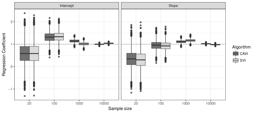
Figure 1: For increasing $n$, boxplots of the cavi and svi solutions for the coefficients in a Bayesian logistic regression with a single covariate. The dotted horizontal line refers to the true coefficients.

To derive the svi routine, let us first express $\mathbb{E}_{q_{\mbox{\tiny opt}}({\bf z})}[{\bm{\eta}}_{1}({\bf y})]-{\bm{\lambda}}_{1}{=}\ 0$ and $\mathbb{E}_{q_{\mbox{\tiny opt}}({\bf z})}[{\bm{\eta}}_{2}({\bf z})]-{\bm{\lambda}}_{2}{=}\ 0$ as

$$\quad\ \ \ {\bm{\Sigma}}_{0}^{-1}{\bm{\mu}}_{0}+\sum\nolimits_{i=1}^{n}{\bf x}_{i}(y_{i}-0.5)-{\bm{\lambda}}_{1}=0,\quad-0.5[{\bm{\Sigma}}_{0}^{-1}+\sum\nolimits_{i=1}^{n}{\bf x}_{i}\mathbb{E}_{q_{\mbox{\tiny opt}}(z_{i})}(z_{i}){\bf x}_{i}^{\intercal}]-{\bm{\lambda}}_{2}=0,$$ (19)

to highlight how the evaluation of (19) requires storing the entire dataset and summing over the whole units. This step could be a major computational bottleneck when the sample size $n$ is massive, thus motivating optimization of $\mathcal{L}({\bm{\lambda}})$ (Hoffman et al., 2013) via stochastic approximation of (19) (Robbins and Monro, 1951). This is done by constructing a random version of $\{{\bm{\Sigma}}_{0}^{-1}{\bm{\mu}}_{0}+\sum\nolimits_{i=1}^{n}{\bf x}_{i}(y_{i}-0.5)-{\bm{\lambda}}_{1},-0.5[{\bm{\Sigma}}_{0}^{-1}+\sum\nolimits_{i=1}^{n}{\bf x}_{i}\mathbb{E}_{q_{\mbox{\tiny opt}}(z_{i})}(z_{i}){\bf x}_{i}^{\intercal}]-{\bm{\lambda}}_{2}\}$ whose expectation coincides with these functions, but its realizations are cheaper to compute. A simple solution is to consider the discrete random variable $B({\bm{\lambda}})$ assuming values $\{B_{i}({\bm{\lambda}}_{1})={\bm{\Sigma}}_{0}^{-1}{\bm{\mu}}_{0}+n{\bf x}_{i}(y_{i}-0.5)-{\bm{\lambda}}_{1},B_{i}({\bm{\lambda}}_{2})=-0.5[{\bm{\Sigma}}_{0}^{-1}+n{\bf x}_{i}\mathbb{E}_{q_{\mbox{\tiny opt}}(z_{i})}(z_{i}){\bf x}_{i}^{\intercal}]-{\bm{\lambda}}_{2}\}$, $i=1,\ldots,n$ with equal probability $n^{-1}$, thus implicitly relying on a mechanism which samples a unit $i$ uniformly and then computes (19) as if such unit was observed $n$ times. This allows application of Robbins and Monro (1951) to solve (19) via the iterative updates

$${\bm{\lambda}}_{1}^{(t)}={\bm{\lambda}}_{1}^{(t-1)}+\rho_{t}B_{t}({\bm{\lambda}}_{1}^{(t-1)}),\quad{\bm{\lambda}}_{2}^{(t)}={\bm{\lambda}}_{2}^{(t-1)}+\rho_{t}B_{t}({\bm{\lambda}}_{2}^{(t-1)}),\qquad\mbox{for every iteration $t$},$$ (20)

where $[B_{t}({\bm{\lambda}}_{1}^{(t-1)}),B_{t}({\bm{\lambda}}_{2}^{(t-1)})]$ is an independent sample of $B({\bm{\lambda}})$, evaluated at $({\bm{\lambda}}_{1}^{(t-1)},{\bm{\lambda}}_{2}^{(t-1)})$, whereas $\rho_{t}$ are step-sizes ensuring convergence to the solution of (19)—and hence to the maximum of $\mathcal{L}({\bm{\lambda}})$—when $\sum_{t}\rho_{t}=+\infty$ and $\sum_{t}\rho^{2}_{t}<+\infty$ (Robbins and Monro, 1951; Spall, 2005). Hoffman et al. (2013) set $\rho_{t}=(t+\tau)^{-\kappa}$, with $\kappa\in(0.5,1]$ denoting the forgetting rate, and $\tau\geq 0$ the delay down-weighting early iterations. These settings ensure the convergence conditions on $\rho_{t}$. Algorithm 3 provides the pseudo–code to perform svi in logistic regression under model (11). As it can be noticed, this routine relies on updating steps which are cheaper to compute than those of cavi. In fact, each iteration of Algorithm 3 does not require to sum over the entire dataset, but relies instead on a single observation sampled uniformly. These gains are fundamental to scale–up calculations in massive datasets.

Figure 1 provides a summarizing quantitative assessment for the performance of cavi and svi in a logistic regression with $\mbox{logit}[\mbox{pr}(y_{i}=1\mid{\bm{\beta}})]=\beta_{1}+\beta_{2}x_{i}$ for each $i=1,\ldots,n$. To study performance under different dimensions, we generate data for increasing sample size $n\in(20,100,1000,10000)$ from a logistic regression with true coefficients $\beta^{(0)}_{1}{=}\ \beta^{(0)}_{2}{=}\ 1$ and covariates $x_{1},\ldots,x_{n}$ from a $\textsc{unif}(-2,2)$. We perform Bayesian inference under a moderately diffuse prior ${\bm{\beta}}\sim\mbox{N}_{2}({\bf 0},10{\cdot}{\bf I}_{2})$ and approximate the posterior via cavi and svi, with $(\tau,\kappa)=(1,0.75)$. As is clear from Figure 1, although svi relies on noisy gradients, the final approximations $q_{\textsc{svi}}^{*}(\beta_{1})$, $q_{\textsc{svi}}^{*}(\beta_{2})$ are similar to the optimal solutions $q^{*}(\beta_{1})$, $q^{*}(\beta_{2})$ from cavi. These approximate posteriors increasingly shrink around the true coefficients as $n$ grows, thus suggesting desirable asymptotic behavior of the cavi and svi solutions. Code and tutorials to reproduce this analysis are available at https://github.com/tommasorigon/logisticVB.

4 Discussion

Motivated by the success of the lower bound developed by Jaakkola and Jordan (2000) for logistic log-likelihoods, and by the lack of formal justifications for its excellent performance, we introduced a novel connection between their construction and a Pólya-gamma data augmentation developed in recent years for logistic regression (Polson, Scott and Windle, 2013). Besides providing a probabilistic interpretation of the bound derived by Jaakkola and Jordan (2000), this connection crucially places the variational methods associated with the proposed lower bound in a more general framework having desirable properties. More specifically, the em for variational inference proposed by Jaakkola and Jordan (2000) maximizes a well–defined elbo associated with a conditionally conjugate exponential family model and, hence, provides the same approximation of the cavi for vb in this model.

The above result motivates further generalizations to novel computational methods, including the svi algorithm in Section 3.2. On a similar line of research, an interesting direction is to incorporate the method of Giordano, Broderick and Jordan (2015) to correct the variance–covariance matrix in $q^{*}({\bm{\beta}})$ from Algorithms 1–3, which is known to underestimate variability. Besides this, the results in Figure 1 motivate also future theoretical studies on the quality of cavi and svi approximations in asymptotic settings. This can be done by adapting available theory on mean–field vb for conditionally conjugate exponential family models (e.g. Wang and Titterington, 2004). Finally, we shall also emphasize that although our focus is on classical Bayesian logistic regression, the results in Sections 2–3 can be easily generalized to more complex learning procedures incorporating logistic models as a building–block, as long as such formulations admit conditionally conjugate exponential family representations.

Appendix A. Maximum likelihood estimation

Although maximum likelihood estimation of the parameters in logistic regression is well–established, there is still active research within this class of models to address other important open questions. For instance, classical Newton–Raphson does not guarantee monotone log-likelihood sequences, thus potentially affecting the stability of the maximization routine (Böhning and Lindsay, 1988). This has motivated other methods leveraging alternative quadratic approximations which uniformly minorize the logistic log-likelihood and are tangent to it (Böhning and Lindsay, 1988; De Leeuw and Lange, 2009; Browne and McNicholas, 2015), thus guaranteeing monotone convergence (Hunter and Lange, 2004). As discussed in Sections 1–2, this is the case of the bound (6) in Jaakkola and Jordan (2000).

Motivated by this result, Jaakkola and Jordan (2000) provided in Appendix C of their article an iterative routine for maximum likelihood estimation of ${\bm{\beta}}$ that has monotone log-likelihood sequences and simple maximizations. In particular, letting ${\bm{\beta}}^{(t-1)}$ denote the estimate of the coefficients at step $t-1$ and simplifying the calculations in Appendix C of Jaakkola and Jordan (2000), their routine first maximizes (6) with respect to $\xi_{1},\ldots,\xi_{n}$, obtaining $\hat{\xi}^{(t-1)}_{i}={\bf x}_{i}^{\intercal}{\bm{\beta}}^{(t-1)}$, $i=1,\ldots,n$, and then derive ${\bm{\beta}}^{(t)}$ by maximizing $\log{\bar{p}}^{(t-1)}({\bf y}\mid{\bm{\beta}})=\sum_{i=1}^{n}\log\bar{p}^{(t-1)}(y_{i}\mid{\bm{\beta}})$, with $\xi_{i}$ replaced by $\hat{\xi}^{(t-1)}_{i}={\bf x}_{i}^{\intercal}{\bm{\beta}}^{(t-1)}$. This last optimization is straightforward to compute due to the quadratic form of (6), thus providing

$${\bm{\beta}}^{(t)}=({\bf X}^{\intercal}\hat{{\bf Z}}^{(t-1)}{\bf X})^{-1}{\bf X}^{\intercal}(y_{1}-0.5,\ldots,y_{n}-0.5)^{\intercal}=({\bf X}^{\intercal}\hat{{\bf Z}}^{(t-1)}{\bf X})^{-1}{\bf X}^{\intercal}({\bf y}-0.5{\cdot}\mbox{\bf 1}_{n}),$$ (21)

with $\hat{{\bf Z}}^{(t-1)}$ a diagonal matrix having entries $\hat{{\bf Z}}^{(t-1)}_{[ii]}=0.5({\bf x}_{i}^{\intercal}{\bm{\beta}}^{(t-1)})^{-1}\mbox{tanh}[0.5({\bf x}_{i}^{\intercal}{\bm{\beta}}^{(t-1)})]$. Analyzing this strategy in the light of (9), it can be noticed that $\hat{\xi}^{(t-1)}_{i}={\bf x}_{i}^{\intercal}{\bm{\beta}}^{(t-1)}$ leads to the solution $\hat{q}^{(t-1)}(z_{i})$ minimizing the kl divergence $\textsc{kl}[q(z_{i})\mid\mid p(z_{i}\mid{\bm{\beta}}^{(t-1)})]$ in (9), for $i=1,\ldots,n$, whereas the function

$$\log{\bar{p}}^{(t-1)}({\bf y}\mid{\bm{\beta}})=\sum_{i=1}^{n}\log{\bar{p}}^{(t-1)}(y_{i}\mid{\bm{\beta}})=\sum_{i=1}^{n}\int_{\Re_{+}}\hat{q}^{(t-1)}(z_{i})\log\frac{p(y_{i}\mid{\bm{\beta}})p(z_{i}\mid{\bm{\beta}})}{\hat{q}^{(t-1)}(z_{i})}\mbox{d}z_{i},$$

maximized with respect to ${\bm{\beta}}$ is equal, up to an additive constant, to the expectation $Q({\bm{\beta}}\mid{\bm{\beta}}^{(t-1)})$ of the complete log-likelihood $\log p({\bf y},{\bf z}\mid{\bm{\beta}})=\sum_{i=1}^{n}\log[p(y_{i}\mid{\bm{\beta}})p(z_{i}\mid{\bm{\beta}})]$ computed with respect to the conditional distribution of the Pólya-gamma data $(z_{i}\mid{\bm{\beta}}^{(t-1)})\sim\textsc{pg}(1,{\bf x}_{i}^{\intercal}{\bm{\beta}}^{(t-1)})$, for $i=1,\ldots,n$. Combining these results with the key rationale underlying em (e.g. Bishop, 2006, Ch. 9.4), it follows that the routine in Appendix C of Jaakkola and Jordan (2000) is an em based on Pólya-gamma augmented data. This algorithm first computes the expectation $Q({\bm{\beta}}\mid{\bm{\beta}}^{(t-1)})=\sum_{i=1}^{n}\mathbb{E}_{\hat{q}^{(t-1)}(z_{i})}\log[p(y_{i}\mid{\bm{\beta}})p(z_{i}\mid{\bm{\beta}})]$ and then maximizes it with respect to ${\bm{\beta}}$. See also Scott and Sun (2013).

As already discussed in Jaakkola and Jordan (2000), the above maximization method guarantees a monotone log-likelihood sequence, thus ensuring a stable convergence. Indeed, leveraging (6) and (9), it can be noticed that the above routine is a genuine minorize-majorize (mm) algorithm (e.g. Hunter and Lange, 2004), provided that $\sum_{i=1}^{n}\log p(y_{i}\mid{\bm{\beta}})\geq\sum_{i=1}^{n}\log{\bar{p}}^{(t-1)}(y_{i}\mid{\bm{\beta}})$ for each ${\bm{\beta}}$, and that $\sum_{i=1}^{n}\log p(y_{i}\mid{\bm{\beta}}^{(t-1)})=\sum_{i=1}^{n}\log{\bar{p}}^{(t-1)}(y_{i}\mid{\bm{\beta}}^{(t-1)})$. We shall notice that also De Leeuw and Lange (2009) and Browne and McNicholas (2015) highlighted this relation with mm under a mathematical argument, while discussing the sharpness of (6). Exploiting results in Section 2, we also show that the mm algorithm relying on (6) improves the convergence rate of the one in Böhning and Lindsay (1988). To our knowledge, this is the only tractable mm alternative to Jaakkola and Jordan (2000).

To address the above goal, let us first re–write (21) to allow a direct comparison with the solution

$${\bm{\beta}}^{(t)}={\bm{\beta}}^{(t-1)}+({\bf X}^{\intercal}{\bm{\Gamma}}{\bf X})^{-1}{\bf X}^{\intercal}(y_{1}-\pi_{1}^{(t-1)},\ldots,y_{n}-\pi_{n}^{(t-1)})^{\intercal},$$ (22)

from Böhning and Lindsay (1988), with ${\bm{\Gamma}}=0.25{\cdot}\mbox{\bf I}_{n}$ and $\pi_{i}^{(t-1)}=[1+\exp(-{{\bf x}}_{i}^{\intercal}{{\bm{\beta}}}^{(t-1)})]^{-1}$. Indeed, by adding and subtracting $\hat{{\bf Z}}^{(t-1)}{\bf X}{\bm{\beta}}^{(t-1)}$ inside $({\bf y}-0.5{\cdot}\mbox{\bf 1}_{n})$, equation (21) coincides with

$${\bm{\beta}}^{(t)}={\bm{\beta}}^{(t-1)}+({\bf X}^{\intercal}\hat{{\bf Z}}^{(t-1)}{\bf X})^{-1}{\bf X}^{\intercal}(y_{1}-\pi_{1}^{(t-1)},\ldots,y_{n}-\pi_{n}^{(t-1)})^{\intercal},$$ (23)

after noticing that each element $y_{i}-0.5-0.5\mbox{tanh}[0.5({{\bf x}}_{i}^{\intercal}{{\bm{\beta}}}^{(t-1)})]$ in ${\bf y}-0.5{\cdot}\mbox{\bf 1}_{n}-\hat{{\bf Z}}^{(t-1)}{\bf X}{\bm{\beta}}^{(t-1)}$ can be alternatively expressed as $y_{i}-0.5\{1+[1-\exp(-{{\bf x}}_{i}^{\intercal}{{\bm{\beta}}}^{(t-1)})][1+\exp(-{{\bf x}}_{i}^{\intercal}{{\bm{\beta}}}^{(t-1)})]^{-1}\}=y_{i}-\pi_{i}^{(t-1)}$. A closer inspection of (22) and (23) shows that the updating underlying Böhning and Lindsay (1988) and Jaakkola and Jordan (2000) coincides with the one from the Newton–Raphson, after replacing the Hessian ${\bf H}^{(t-1)}=-{\bf X}^{\intercal}{\bm{\Lambda}}^{(t-1)}{\bf X}=-{\bf X}^{\intercal}\mbox{diag}[\pi^{(t-1)}_{1}(1-\pi^{(t-1)}_{1}),\ldots,\pi^{(t-1)}_{n}(1-\pi^{(t-1)}_{n})]{\bf X}$—evaluated in ${\bm{\beta}}^{(t-1)}$—of the logistic log-likelihood, with $-{\bf X}^{\intercal}{\bm{\Gamma}}{\bf X}$ in (22) and $-{\bf X}^{\intercal}\hat{{\bf Z}}^{(t-1)}{\bf X}$ in (23). Recalling Böhning and Lindsay (1988), both matrices define a lower bound for the Hessian and guarantee that both (22) and (23) induce a monotone sequence for the log-likelihood. In Böhning and Lindsay (1988) the uniform bound follows after noticing that ${\bm{\pi}}^{(t-1)}(1-{\bm{\pi}}^{(t-1)})\leq 0.25{\cdot}\mbox{\bf 1}_{n}$ for any ${\bm{\pi}}^{(t-1)}\in(0,1)^{n}$, whereas, according to Lemma 1, the adaptive bound induced by Jaakkola and Jordan (2000) is formally related to an exact data augmentation, thus suggesting that (23) may provide more efficient updates than (22). This claim is formalized in Proposition 1 by comparing the convergence rates of the two algorithms. Refer to McLachlan and Krishnan (2007, Chapter 3.9) for details regarding the definition and the computation of the convergence rate associated with a generic iterative routine.

Proposition 1.

Assume that ${\bm{\beta}}^{*}$ is the limit, if it exists, of $\{{\bm{\beta}}^{(t)}:t\geq 1\}$, and let $\mbox{M}^{\textsc{b}}(\cdot)=\{\mbox{M}_{1}^{\textsc{b}}(\cdot),\ldots,\mbox{M}_{p}^{\textsc{b}}(\cdot)\}$ and $\mbox{M}^{\textsc{j}}(\cdot)=\{\mbox{M}_{1}^{\textsc{j}}(\cdot),\ldots,\mbox{M}_{p}^{\textsc{j}}(\cdot)\}$ denote the functions mapping from ${\bm{\beta}}^{(t-1)}$ to ${\bm{\beta}}^{(t)}$ in (22) and (23), respectively. Then $r_{\textsc{b}}\geq r_{\textsc{j}}$, with $r_{\textsc{b}}=||\bm{J}_{\textsc{b}}^{*}||_{2}$ and $r_{\textsc{j}}=||\bm{J}_{\textsc{j}}^{*}||_{2}$ being the maximum eigenvalues of the Jacobians $\bm{J}_{\textsc{b}}=\partial\mbox{M}^{\textsc{b}}({\bm{\beta}})/\partial{\bm{\beta}}$ and $\bm{J}_{\textsc{j}}=\partial\mbox{M}^{\textsc{j}}({\bm{\beta}})/\partial{\bm{\beta}}$, respectively, computed in ${\bm{\beta}}^{*}$.

To prove Proposition 1, note that $\bm{J}_{\textsc{b}}^{*}={\bf I}_{p}+({\bf X}^{\intercal}{\bm{\Gamma}}{\bf X})^{-1}{\bf H}^{*}$ can be easily computed as in Böhning and Lindsay (1988), since ${\bm{\Gamma}}$ does not depend on ${\bm{\beta}}$ in (22). It is instead not immediate to calculate $\bm{J}_{\textsc{j}}^{*}$ via direct differentiation of $\mbox{M}^{\textsc{j}}({\bm{\beta}})$, because (23) contains more complex hyperbolic transformations of ${\bm{\beta}}$. However, exploiting the probabilistic findings in Section 2, this issue can be easily circumvented leveraging the em interpretation of the routine in Jaakkola and Jordan (2000) via Pólya-gamma augmented data. Indeed, following McLachlan and Krishnan (2007, Ch. 3.9.3), the rate matrix of an iterative routine based on em methods, is equal to $\bm{J}_{\textsc{j}}^{*}=\mbox{\bf I}_{p}+\mathcal{I}_{c}({\bm{\beta}}^{*})^{-1}{\bf H}^{*}$, with $\mathcal{I}_{c}({\bm{\beta}}^{*})$ denoting the expectation, taken with respect to the augmented data, of the complete-data information matrix $\mbox{I}_{c}({\bm{\beta}}^{*})$. This quantity can be easily computed in our case, provided that the complete log-likelihood is equal, up to an additive constant, to the quadratic function $\sum_{i=1}^{n}\{(y_{i}-0.5){\bf x}_{i}^{\intercal}{\bm{\beta}}-0{.5}z_{i}({\bf x}_{i}^{\intercal}{\bm{\beta}})^{2}\}$ of ${\bm{\beta}}$, which is also linear in the augmented Pólya-gamma data $z_{i}$. Due to this, it is easy to show that $\mathcal{I}_{c}({\bm{\beta}}^{*})={\bf X}^{\intercal}\hat{{\bf Z}}^{*}{\bf X}$, where $\hat{{\bf Z}}^{*}$ is the $n\times n$ diagonal matrix with entries $\hat{{\bf Z}}_{[ii]}^{*}=0.5({\bf x}_{i}^{\intercal}{\bm{\beta}}^{*})^{-1}\mbox{tanh}\{0{.}5({\bf x}_{i}^{\intercal}{\bm{\beta}}^{*})\}$.

Proof.

Recalling the above discussion, the proof of Proposition 1 requires comparing the maximum eigenvalues of $\bm{J}_{\textsc{b}}^{*}=\mbox{\bf I}_{p}+({\bf X}^{\intercal}{\bm{\Gamma}}{\bf X})^{-1}{\bf H}^{*}=\mbox{\bf I}_{p}-({\bf X}^{\intercal}{\bm{\Gamma}}{\bf X})^{-1}({\bf X}^{\intercal}{\bm{\Lambda}}^{*}{\bf X})$ and $\bm{J}_{\textsc{j}}^{*}=\mbox{\bf I}_{p}+({\bf X}^{\intercal}\hat{{\bf Z}}^{*}{\bf X})^{-1}{\bf H}^{*}=\mbox{\bf I}_{p}-({\bf X}^{\intercal}\hat{{\bf Z}}^{*}{\bf X})^{-1}({\bf X}^{\intercal}{\bm{\Lambda}}^{*}{\bf X})$. To address this goal, let us first show that $\bm{J}_{\textsc{b}}^{*}\geq\bm{J}_{\textsc{j}}^{*}$. This result can be proved by noticing that $\bm{J}_{\textsc{b}}^{*}$ and $\bm{J}_{\textsc{j}}^{*}$ only differ by the positive diagonal matrices ${\bm{\Gamma}}$ and $\hat{{\bf Z}}^{*}$, respectively. Hence, the above inequality is met if all the entries ${\bm{\Gamma}}_{[ii]}-\hat{{\bf Z}}^{*}_{[ii]}=0.25-0.5({\bf x}_{i}^{\intercal}{\bm{\beta}}^{*})^{-1}\mbox{tanh}\{0.5({\bf x}_{i}^{\intercal}{\bm{\beta}}^{*})\}=0.25[1-2({\bf x}_{i}^{\intercal}{\bm{\beta}}^{*})^{-1}\mbox{tanh}\{0{.}5({\bf x}_{i}^{\intercal}{\bm{\beta}}^{*})\}]$ in the diagonal matrix ${\bm{\Gamma}}-\hat{{\bf Z}}^{*}$ are non-negative. Letting $u=0.5({\bf x}_{i}^{\intercal}{\bm{\beta}}^{*})$, and re–writing the well–established inequality $u^{-1}\mbox{sinh}(u)\leq\mbox{cosh}(u)$ (e.g. Zhu, 2012) as $u^{-1}\mbox{sinh}(u)\mbox{cosh}^{-1}(u)\leq 1$, it follows that $u^{-1}\mbox{tanh}(u)=2({\bf x}_{i}^{\intercal}{\bm{\beta}}^{*})^{-1}\mbox{tanh}\{0.5({\bf x}_{i}^{\intercal}{\bm{\beta}}^{*})\}\leq 1$, thus guaranteeing ${\bm{\Gamma}}-\hat{{\bf Z}}^{*}\geq 0$, and, as a direct consequence, $\bm{J}_{\textsc{b}}^{*}\geq\bm{J}_{\textsc{j}}^{*}$. This concludes the proof. In fact, $\bm{J}_{\textsc{b}}^{*}\geq\bm{J}_{\textsc{j}}^{*}$ implies $||\bm{J}_{\textsc{b}}^{*}||_{2}=r_{\textsc{b}}\geq r_{\textsc{j}}=||\bm{J}_{\textsc{j}}^{*}||_{2}$ (e.g. Knutson and Tao, 2001). ∎

Proposition 1 ensures that (23) improves the convergence rate of (22). In fact, higher values of $r$ imply slower convergence. We shall however emphasize that the em in Appendix C of Jaakkola and Jordan (2000) does not reach the quadratic convergence of Newton–Raphson, but guarantees monotone log-likelihood sequences. It is also important to highlight that although the mm in Böhning and Lindsay (1988) has slower convergence, the matrix ${\bf X}^{\intercal}{\bm{\Gamma}}{\bf X}$ in (22) does not depend on ${\bm{\beta}}^{(t-1)}$, thus requiring inversion only once during the iterative procedure. This reduces computational complexity, especially in high–dimensional problems, compared to the updating in (23), which requires, instead, inversion of ${\bf X}^{\intercal}\hat{{\bf Z}}^{(t-1)}{\bf X}$ at each iteration. We refer to the tutorial em_logistic_tutorial.md in https://github.com/tommasorigon/logisticVB for illustrative simulations providing a quantitative comparison among the aforementioned methods.

Although the above focus has been on maximum likelihood estimation methods, the probabilistic interpretation (8) of the quadratic bound in Jaakkola and Jordan (2000) motivates simple adaptations to include the maximum a posteriori estimation problem under a Bayesian framework. This routine has been carefully studied by Scott and Sun (2013) and we refer to their contribution for details.

References

• Airoldi et al. (2008) {barticle}[author] \bauthor\bsnmAiroldi, \bfnmEdoardo M\binitsE. M., \bauthor\bsnmBlei, \bfnmDavid M\binitsD. M., \bauthor\bsnmFienberg, \bfnmStephen E\binitsS. E. and \bauthor\bsnmXing, \bfnmEric P\binitsE. P. (\byear2008). \btitleMixed membership stochastic blockmodels. \bjournalJ. Mach. Learn. Res. \bvolume9 \bpages1981–2014. \endbibitem
• Beal and Ghahramani (2003) {barticle}[author] \bauthor\bsnmBeal, \bfnmM. J.\binitsM. J. and \bauthor\bsnmGhahramani, \bfnmZoubin\binitsZ. (\byear2003). \btitleThe variational Bayesian EM algorithm for incomplete data: with application to scoring graphical model structures. \bjournalBayesian Stat. \bvolume7 \bpages453–464. \endbibitem
• Bishop (2006) {bbook}[author] \bauthor\bsnmBishop, \bfnmChristopher M\binitsC. M. (\byear2006). \btitlePattern Recognition and Machine Learning. \bpublisherSpringer. \endbibitem
• Bishop and Svensén (2003) {barticle}[author] \bauthor\bsnmBishop, \bfnmChristopher M\binitsC. M. and \bauthor\bsnmSvensén, \bfnmMarkus\binitsM. (\byear2003). \btitleBayesian hierarchical mixtures of experts. \bjournalProceedings of the Conference on Uncertainty in Artificial Intelligence \bpages57–64. \endbibitem
• Blei, Kucukelbir and McAuliffe (2017) {barticle}[author] \bauthor\bsnmBlei, \bfnmDavid M\binitsD. M., \bauthor\bsnmKucukelbir, \bfnmAlp\binitsA. and \bauthor\bsnmMcAuliffe, \bfnmJon D\binitsJ. D. (\byear2017). \btitleVariational inference: A review for statisticians. \bjournalJ. Amer. Statist. Assoc. \bvolume112 \bpages859–877. \endbibitem
• Blei, Ng and Jordan (2003) {barticle}[author] \bauthor\bsnmBlei, \bfnmDavid M\binitsD. M., \bauthor\bsnmNg, \bfnmAndrew Y\binitsA. Y. and \bauthor\bsnmJordan, \bfnmMichael I\binitsM. I. (\byear2003). \btitleLatent dirichlet allocation. \bjournalJ. Mach. Learn. Res. \bvolume3 \bpages993–1022. \endbibitem
• Böhning and Lindsay (1988) {barticle}[author] \bauthor\bsnmBöhning, \bfnmDankmar\binitsD. and \bauthor\bsnmLindsay, \bfnmBruce G\binitsB. G. (\byear1988). \btitleMonotonicity of quadratic-approximation algorithms. \bjournalAnn. I. Stat. Math. \bvolume40 \bpages641–663. \endbibitem
• Braun and McAuliffe (2010) {barticle}[author] \bauthor\bsnmBraun, \bfnmMichael\binitsM. and \bauthor\bsnmMcAuliffe, \bfnmJon\binitsJ. (\byear2010). \btitleVariational inference for large-scale models of discrete choice. \bjournalJ. Amer. Statist. Assoc. \bvolume105 \bpages324–335. \endbibitem
• Browne and McNicholas (2015) {barticle}[author] \bauthor\bsnmBrowne, \bfnmRyan P\binitsR. P. and \bauthor\bsnmMcNicholas, \bfnmPaul D\binitsP. D. (\byear2015). \btitleMultivariate sharp quadratic bounds via $\Sigma$-strong convexity and the Fenchel connection. \bjournalElectron. J. Stat. \bvolume9 \bpages1913–1938. \endbibitem
• Carbonetto and Stephens (2012) {barticle}[author] \bauthor\bsnmCarbonetto, \bfnmPeter\binitsP. and \bauthor\bsnmStephens, \bfnmMatthew\binitsM. (\byear2012). \btitleScalable variational inference for Bayesian variable selection in regression, and its accuracy in genetic association studies. \bjournalBayesian Anal. \bvolume7 \bpages73–108. \endbibitem
• Choi and Hobert (2013) {barticle}[author] \bauthor\bsnmChoi, \bfnmHee Min\binitsH. M. and \bauthor\bsnmHobert, \bfnmJames P\binitsJ. P. (\byear2013). \btitleThe Polya-gamma Gibbs sampler for Bayesian logistic regression is uniformly ergodic. \bjournalElectron. J. Stat. \bvolume7 \bpages2054–2064. \endbibitem
• De Leeuw and Lange (2009) {barticle}[author] \bauthor\bsnmDe Leeuw, \bfnmJan\binitsJ. and \bauthor\bsnmLange, \bfnmKenneth\binitsK. (\byear2009). \btitleSharp quadratic majorization in one dimension. \bjournalComput. Statist. Data Anal. \bvolume53 \bpages2471–2484. \endbibitem
• Dempster, Laird and Rubin (1977) {barticle}[author] \bauthor\bsnmDempster, \bfnmArthur P\binitsA. P., \bauthor\bsnmLaird, \bfnmNan M\binitsN. M. and \bauthor\bsnmRubin, \bfnmDonald B\binitsD. B. (\byear1977). \btitleMaximum likelihood from incomplete data via the EM algorithm. \bjournalJ. R. Stat. Soc. Ser. B. Stat. Methodol. \bvolume39 \bpages1–38. \endbibitem
• Gelfand and Smith (1990) {barticle}[author] \bauthor\bsnmGelfand, \bfnmAlan E\binitsA. E. and \bauthor\bsnmSmith, \bfnmAdrian FM\binitsA. F. (\byear1990). \btitleSampling-based approaches to calculating marginal densities. \bjournalJ. Amer. Statist. Assoc. \bvolume85 \bpages398–409. \endbibitem
• Giordano, Broderick and Jordan (2015) {barticle}[author] \bauthor\bsnmGiordano, \bfnmRyan J\binitsR. J., \bauthor\bsnmBroderick, \bfnmTamara\binitsT. and \bauthor\bsnmJordan, \bfnmMichael I\binitsM. I. (\byear2015). \btitleLinear response methods for accurate covariance estimates from mean field variational Bayes. \bjournalAdvances in Neural Information Processing Systems \bpages1441–1449. \endbibitem
• Hoffman et al. (2013) {barticle}[author] \bauthor\bsnmHoffman, \bfnmMatthew D\binitsM. D., \bauthor\bsnmBlei, \bfnmDavid M\binitsD. M., \bauthor\bsnmWang, \bfnmChong\binitsC. and \bauthor\bsnmPaisley, \bfnmJohn\binitsJ. (\byear2013). \btitleStochastic variational inference. \bjournalJ. Mach. Learn. Res. \bvolume14 \bpages1303–1347. \endbibitem
• Hunter and Lange (2004) {barticle}[author] \bauthor\bsnmHunter, \bfnmDavid R\binitsD. R. and \bauthor\bsnmLange, \bfnmKenneth\binitsK. (\byear2004). \btitleA tutorial on MM algorithms. \bjournalAm. Stat. \bvolume58 \bpages30–37. \endbibitem
• Jaakkola and Jordan (2000) {barticle}[author] \bauthor\bsnmJaakkola, \bfnmTommi S\binitsT. S. and \bauthor\bsnmJordan, \bfnmMichael I\binitsM. I. (\byear2000). \btitleBayesian parameter estimation via variational methods. \bjournalStat. Comput. \bvolume10 \bpages25–37. \endbibitem
• Jordan et al. (1999) {barticle}[author] \bauthor\bsnmJordan, \bfnmMichael I\binitsM. I., \bauthor\bsnmGhahramani, \bfnmZoubin\binitsZ., \bauthor\bsnmJaakkola, \bfnmTommi S\binitsT. S. and \bauthor\bsnmSaul, \bfnmLawrence K\binitsL. K. (\byear1999). \btitleAn introduction to variational methods for graphical models. \bjournalMach. Learn. \bvolume37 \bpages183–233. \endbibitem
• Knutson and Tao (2001) {barticle}[author] \bauthor\bsnmKnutson, \bfnmAllen\binitsA. and \bauthor\bsnmTao, \bfnmTerence\binitsT. (\byear2001). \btitleHoneycombs and sums of Hermitian matrices. \bjournalNot. Am. Math. Soc. \bvolume48 \bpages175–186. \endbibitem
• Kullback and Leibler (1951) {barticle}[author] \bauthor\bsnmKullback, \bfnmSolomon\binitsS. and \bauthor\bsnmLeibler, \bfnmRichard A\binitsR. A. (\byear1951). \btitleOn information and sufficiency. \bjournalAnn. Math. Stat. \bvolume22 \bpages79–86. \endbibitem
• Lee, Huang and Hu (2010) {barticle}[author] \bauthor\bsnmLee, \bfnmSeokho\binitsS., \bauthor\bsnmHuang, \bfnmJianhua Z.\binitsJ. Z. and \bauthor\bsnmHu, \bfnmJianhua\binitsJ. (\byear2010). \btitleSparse logistic principal components analysis for binary data. \bjournalAnn. Appl. Stat. \bvolume4 \bpages1579–1601. \endbibitem
• McLachlan and Krishnan (2007) {bbook}[author] \bauthor\bsnmMcLachlan, \bfnmG.\binitsG. and \bauthor\bsnmKrishnan, \bfnmT.\binitsT. (\byear2007). \btitleThe EM Algorithm and Extensions. \bpublisherWiley. \endbibitem
• Ormerod and Wand (2010) {barticle}[author] \bauthor\bsnmOrmerod, \bfnmJohn T\binitsJ. T. and \bauthor\bsnmWand, \bfnmMatt P\binitsM. P. (\byear2010). \btitleExplaining variational approximations. \bjournalAm. Stat. \bvolume64 \bpages140–153. \endbibitem
• Polson, Scott and Windle (2013) {barticle}[author] \bauthor\bsnmPolson, \bfnmNicholas G\binitsN. G., \bauthor\bsnmScott, \bfnmJames G\binitsJ. G. and \bauthor\bsnmWindle, \bfnmJesse\binitsJ. (\byear2013). \btitleBayesian inference for logistic models using Pólya–Gamma latent variables. \bjournalJ. Amer. Statist. Assoc. \bvolume108 \bpages1339–1349. \endbibitem
• Rasmussen and Williams (2006) {bbook}[author] \bauthor\bsnmRasmussen, \bfnmC E\binitsC. E. and \bauthor\bsnmWilliams, \bfnmC K\binitsC. K. (\byear2006). \btitleGaussian Processes for Machine Learning. \bpublisherMIT Press. \endbibitem
• Ren et al. (2011) {barticle}[author] \bauthor\bsnmRen, \bfnmLu\binitsL., \bauthor\bsnmDu, \bfnmLan\binitsL., \bauthor\bsnmCarin, \bfnmLawrence\binitsL. and \bauthor\bsnmDunson, \bfnmDavid B.\binitsD. B. (\byear2011). \btitleLogistic stick-breaking process. \bjournalJ. Mach. Learn. Res. \bvolume12 \bpages203–239. \endbibitem
• Robbins and Monro (1951) {barticle}[author] \bauthor\bsnmRobbins, \bfnmHerbert\binitsH. and \bauthor\bsnmMonro, \bfnmSutton\binitsS. (\byear1951). \btitleA stochastic approximation method. \bjournalAnn. Math. Stat. \bvolume22 \bpages400–407. \endbibitem
• Scott and Sun (2013) {barticle}[author] \bauthor\bsnmScott, \bfnmJames G\binitsJ. G. and \bauthor\bsnmSun, \bfnmLiang\binitsL. (\byear2013). \btitleExpectation-maximization for logistic regression. \bjournalarXiv:1306.0040. \endbibitem
• Spall (2005) {bbook}[author] \bauthor\bsnmSpall, \bfnmJames C\binitsJ. C. (\byear2005). \btitleIntroduction to Stochastic Search and Optimization: Estimation, Simulation, and Control. \bpublisherJohn Wiley & Sons. \endbibitem
• Tang, Browne and McNicholas (2015) {barticle}[author] \bauthor\bsnmTang, \bfnmYang\binitsY., \bauthor\bsnmBrowne, \bfnmRyan P.\binitsR. P. and \bauthor\bsnmMcNicholas, \bfnmPaul D.\binitsP. D. (\byear2015). \btitleModel based clustering of high-dimensional binary data. \bjournalComput. Statist. Data Anal. \bvolume87 \bpages84–101. \endbibitem
• Wand (2017) {barticle}[author] \bauthor\bsnmWand, \bfnmMatt P\binitsM. P. (\byear2017). \btitleFast approximate inference for arbitrarily large semiparametric regression models via message passing. \bjournalJ. Amer. Statist. Assoc. \bvolume112 \bpages137–168. \endbibitem
• Wand et al. (2011) {barticle}[author] \bauthor\bsnmWand, \bfnmMatthew P\binitsM. P., \bauthor\bsnmOrmerod, \bfnmJohn T\binitsJ. T., \bauthor\bsnmPadoan, \bfnmSimone A\binitsS. A. and \bauthor\bsnmFrühwirth, \bfnmRudolf\binitsR. (\byear2011). \btitleMean field variational Bayes for elaborate distributions. \bjournalBayesian Anal. \bvolume6 \bpages847–900. \endbibitem
• Wang and Blei (2013) {barticle}[author] \bauthor\bsnmWang, \bfnmChong\binitsC. and \bauthor\bsnmBlei, \bfnmDavid M\binitsD. M. (\byear2013). \btitleVariational inference in nonconjugate models. \bjournalJ. Mach. Learn. Res. \bvolume14 \bpages1005–1031. \endbibitem
• Wang and Titterington (2004) {barticle}[author] \bauthor\bsnmWang, \bfnmBo\binitsB. and \bauthor\bsnmTitterington, \bfnmD Michael\binitsD. M. (\byear2004). \btitleConvergence and asymptotic normality of variational Bayesian approximations for exponential family models with missing values. \bjournalProceedings of the Conference on Uncertainty in Artificial Intelligence \bpages577–584. \endbibitem
• Zhu (2012) {barticle}[author] \bauthor\bsnmZhu, \bfnmLing\binitsL. (\byear2012). \btitleNew inequalities for hyperbolic functions and their applications. \bjournalJ. Inequal. Appl. \bvolume303 \bpages1–29. \endbibitem