Deconstructing the Gel’fand–Yaglom method and vacuum energy from a theory space

Abstract

The discrete Gel’fand–Yaglom theorem was studied several years ago. In the present paper, we generalize the discrete Gel’fand–Yaglom method to obtain the determinants of mass matrices which appear current works in particle physics, such as dimensional deconstruction and clockwork theory. Using the results, we show the expressions for vacuum energies in such various models.
PACS: 02.10.Ox, 04.60.Nc, 11.10.Kk, 11.25.Mj.

1 Introduction

The Gel’fand–Yaglom method [1] for obtaining functional determinants of differential operators with boundaries is widely known nowadays. For nice reviews, see [2, 3]. The applications of the Gel’fand–Yaglom method have been investigated quite recently, to evaluate one-loop vacuum energies in nontrivial boundary conditions [4, 5, 6, 7].

Among them, Altshuler examined vacuum energy in warped compactification [6, 7]. In recent years, it is supposed that extra dimensions of various types could play an important role in the hierarchy problem, and thus the study of physics in nontrivial background geometry is still advancing.

The dimensional deconstruction has appeared as a new tool for understanding the properties of higher-dimensional field theories [8, 9, 10] more than a decade ago. In such a model of deconstruction, a ‘theory space’ is considered, which consists of sites and links, to which four-dimensional fields are individually assigned. Theory spaces thus have the structures of graphs [11] and can be interpreted as the theory with discrete extra dimensions.

Several years ago, the discrete Gel’fand–Yaglom method for difference operators was reviewed and studied by Dowker [12]. We generalize the discrete Gel’fand–Yaglom method for studying one-loop vacuum energies in extended deconstructed theories and models with discrete dimensions in the present paper. To this ends, we develop the method of computing determinants of repetitive Hermitian matrices which correspond to mass matrices utilized in deconstructed theories.

After completion of the first version of the manuscript of the present paper (arXiv:1711.06806), a paper which treats the determinants of discrete Laplace operators appeared [13]. Their method is substantially the same as ours, because the author also relies on the recurrence relation among three variables on a lattice (see Sec. 3 in the present paper and below). We recently become aware of another similar paper on the determinants of matrix differential operators [14]. They studied generalization of Gel’fand–Yaglom method to obtain the functional determinants. Their work differs essentially from ours because they considered differential operators while we treat matrices as operators. We also point out that they did not consider the matrices of large size which have certain continuum limits.

The organization of this paper is as follows. In order to make the present paper self-contained, we show a short review of the Gel’fand–Yaglom method for a differential operator, along with the Dunne’s review [2], in Sec. 2. In Sec. 3, we give the method to obtain determinants of tridiagonal matrices with repeated structure. This is a straightforward generalization of description in Ref. [12]. In Sec. 4, we give the method to obtain determinants of periodic tridiagonal matrices. Determinants of extended periodic tridiagonal matrices are obtained in Sec. 5. The rest of the present paper is devoted to applications to deconstructed theories and discrete systems. In Sec. 6, free energy on a graph is discussed by using the results of previous sections. In Sec. 7, we show the method of calculation for evaluating one-loop vacuum energy in deconstructed models from the determinants of mass matrices. In Sec. 8, we show a few more examples of one-loop vacuum energies for slightly complicated theory spaces. We give conclusions in the last section, Sec. 9.

2 Review of the Gel’fand–Yaglom method [2]

Suppose that an eigenvalue equation $(\Delta+m^{2})\psi^{(m^{2})}_{\lambda}(x)=\lambda^{(m^{2})}\psi^{(m^{2})}_{\lambda}(x)$ with Dirichlet-Dirichlet boundary conditions $\psi^{(m^{2})}_{\lambda}(0)=\psi^{(m^{2})}_{\lambda}(L)=0$ in one dimension is given.

Then

$$\frac{\det[\Delta+m^{2}]}{\det[\Delta]}=\frac{\psi^{(m^{2})}_{0}(L)}{\psi^{(0)}_{0}(L)}\,,$$ (1)

holds. Here $\psi^{(m^{2})}_{0}(x)$ satisfies $(\Delta+m^{2})\psi^{(m^{2})}_{0}(x)=0$ with a boundary condition $\psi^{(m^{2})}_{0}(0)=0$.

example

In the region $0\leq x\leq L$, under the Dirichlet condition at the boundaries, we consider the functional determinant

$$\frac{\det[-\partial_{x}^{2}+m^{2}]}{\det[-\partial_{x}^{2}]}\,.$$ (2)

The solution of $(-\partial_{x}^{2}+m^{2})\psi(x)=0$ with $\psi(0)=0$ is $\sinh mx$. Thus according to the Gel’fand–Yaglom method, we obtain

$$\frac{\det[-\partial_{x}^{2}+m^{2}]}{\det[-\partial_{x}^{2}]}=\frac{\sinh mL}{mL}=\prod_{n=1}^{\infty}\frac{\frac{n^{2}\pi^{2}}{L^{2}}+m^{2}}{\frac{n^{2}\pi^{2}}{L^{2}}}\,.$$ (3)

proof

$\det[\Delta+m^{2}-\lambda]$ is a function of $\lambda$ and has zeros at $\lambda=\lambda^{(m^{2})}$. The function $\psi_{\lambda}(x)$ which satisfies $(\Delta+m^{2}-\lambda)\psi_{\lambda}(x)=0$ and $\psi_{\lambda}(0)=0$ becomes the eigenfunction when $\lambda=\lambda^{(m^{2})}$. Then the boundary condition at $x=L$, i.e., $\psi_{\lambda}(L)=0$ is satisfied. In other words, $\psi_{\lambda}(L)$ is a function of $\lambda$ and has zeros at $\lambda=\lambda^{(m^{2})}$. Therefore $\det[\Delta+m^{2}-\lambda]\propto\psi_{\lambda}(L)$ holds. 

3 Determinants of tridiagonal matrices

3.1 the discrete Gel’fand–Yaglom method for tridiagonal matrices

Now, we show the disctrete Gel’fand–Yaglom method to obtain determinants of finite matrices. First, we consider the following Hermitian tridiagonal matrix of $N$ rows and columns:

$$H=\left(\begin{array}[]{cccccc}c&-b&0&\cdots&&0\\ -b^{*}&a&-b&\cdots&&0\\ 0&-b^{*}&a&\cdots&&0\\ \vdots&\vdots&\vdots&\ddots&&\vdots\\ &&&&a&-b\\ 0&0&0&\cdots&-b^{*}&d\end{array}\right)\,.$$ (4)

In this case, the eigenvalue equation

$$H\mathbf{v}=\lambda\mathbf{v}\,,$$ (5)

where $\mathbf{v}^{T}=(v_{1},v_{2},\dots,v_{N})$, can be categorized into three parts,

$$\sum_{j=1}^{N}H_{1j}v_{j}-\lambda v_{1}=0\,,$$ (6)

$$\sum_{j=1}^{N}H_{kj}v_{j}-\lambda v_{k}=0\quad(2\leq k\leq N-1)\,,$$ (7)

$$\sum_{j=1}^{N}H_{Nj}v_{j}-\lambda v_{N}=0\,.$$ (8)

Here, Eq. (7) is just the recurrence relation among three terms in $v_{k}$ as a sequence of numbers. In the present case, the general solution for the recurrence relation

$$bv_{k+1}-(a-\lambda)v_{k}+b^{*}v_{k-1}=0\quad(2\leq k\leq N-1)$$ (9)

is

$$v_{k}=A\alpha^{k-1}+B\beta^{k-1}\,,$$ (10)

where $A$ and $B$ are constants and

$$\alpha=\frac{a-\lambda+\sqrt{(a-\lambda)^{2}-4|b|^{2}}}{2b}\,,\quad\beta=\frac{a-\lambda-\sqrt{(a-\lambda)^{2}-4|b|^{2}}}{2b}\,.$$ (11)

Note that $\alpha$ and $\beta$ are roots of the second-order equation $bx^{2}-(a-\lambda)x+b^{*}=0$ and $\alpha\beta=b^{*}/b$.

The first row of the eigenvalue equation, Eq. (6), determines the relation between $v_{1}$ and $v_{2}$; in this case, that is $(c-\lambda)v_{1}-bv_{2}=0$. If we further choose

$$v_{1}=A+B=1\,,$$ (12)

the coefficients $A$ and $B$ are obtained as

$$A=A(\lambda)=\frac{c-\lambda-b\beta}{b(\alpha-\beta)}=\frac{c-\lambda-b\beta}{\sqrt{(a-\lambda)^{2}-4|b|^{2}}}\,,$$ (13)

$$B=B(\lambda)=\frac{-(c-\lambda-b\alpha)}{b(\alpha-\beta)}=\frac{-(c-\lambda-b\alpha)}{\sqrt{(a-\lambda)^{2}-4|b|^{2}}}\,.$$ (14)

Substituting all of the results above into Eq. (8) in the present case, we get

$$A(\lambda)[-b^{*}+(d-\lambda)\alpha]\alpha^{N-2}+B(\lambda)[-b^{*}+(d-\lambda)\beta]\beta^{N-2}=0\,.$$ (15)

Now, we set the left-hand side of Eq. (15) as $\tilde{D}(\lambda)$. $\tilde{D}(\lambda)$ is zero if $\lambda$ is an eigenvalue of the matrix $H$ in this case. By construction, $\tilde{D}(\lambda)$ should be an $N$th order polynomial of $\lambda$. The reason is: $v_{2}=[(c-\lambda)/b]v_{1}=(c-\lambda)/b$, $v_{3}=[(a-\lambda)/b]v_{2}-(b^{*}/b)v_{1}=(a-\lambda)(c-\lambda)/b^{2}-(b^{*}/b)$, and so on. This observation shows $v_{N}$ includes $(-{\lambda})^{N-1}/b^{N-1}$. Finally, since the left-hand side of Eq. (8) reads $-b^{*}v_{N-1}+(d-\lambda)v_{N}$ in the present case, $\tilde{D}(\lambda)$ has the term $(-{\lambda})^{N}/b^{N-1}$ as the highest order term in $\lambda$. We can also directly confirm this by setting $a=c=d=0$ and the limit $b\rightarrow 0$ in the left-hand side of Eq. (15). We then verify $\tilde{D}(\lambda)\rightarrow(-{\lambda})^{N}/b^{N-1}$.

Therefore, we conclude that $D(\lambda)=b^{N-1}\tilde{D}(\lambda)=\prod_{p=1}^{N}(\lambda_{p}-\lambda)$ is the characteristic polynomial of $H$, where $\lambda_{p}$ $(p=1,2,\dots,N)$ are eigenvalues of $H$.

The determinant of $H$ is given by $D(0)=\prod_{p=1}^{N}\lambda_{p}$. In the present case, we find

$$\det H=D(0)=\frac{b^{N-1}}{\sqrt{a^{2}-4|b|^{2}}}\Big{[}(c-b\bar{\beta})(-b^{*}+d\bar{\alpha})\bar{\alpha}^{N-2}-(c-b\bar{\alpha})(-b^{*}+d\bar{\beta})\bar{\beta}^{N-2}\Big{]}\,,$$ (16)

where

$$\bar{\alpha}=\frac{a+\sqrt{a^{2}-4|b|^{2}}}{2b}\,,\quad\bar{\beta}=\frac{a-\sqrt{a^{2}-4|b|^{2}}}{2b}\,.$$ (17)

After a lengthy calculation, we obtain

$$\det H=D(0)$$ (18)

$$= \frac{1}{2^{N}\sqrt{a^{2}-4|b|^{2}}}\Big{\{}\Big{[}2(cd-|b|^{2})+(a-c-d)(a-\sqrt{a^{2}-4|b|^{2}})\Big{]}(a+\sqrt{a^{2}-4|b|^{2}})^{N-1}$$

$$-\Big{[}2(cd-|b|^{2})+(a-c-d)(a+\sqrt{a^{2}-4|b|^{2}})\Big{]}(a-\sqrt{a^{2}-4|b|^{2}})^{N-1}\Big{\}}\,$$

$$\qquad\mbox{(for a tridiagonal matrix)}\,,$$

in the present case. It is notable that the determinant depends only on $|b|$ and does not depend on $b^{*}/b$ in the present case. The reason is because the eigenvalues are unchanged under “gauge” transformation $\mathbf{v}\rightarrow P\mathbf{v}$ and $H\rightarrow PHP^{-1}$, where $P=diag.(1,e^{i\chi},e^{i2\chi},\ldots,e^{i(N-1)\chi})$ with an arbitrary real constant $\chi$.

The prescription of the above method to obtain the determinant is very similar to the Gel’fand–Yaglom method for differential operators. Namely, solving the differential equation corresponds to solving the recurrence relation, putting one of the boundary conditions corresponds to fixing the first term of the series of numbers, and obtaining the determinant at another boundary corresponds to obtaining the determinant as the equation of the last row in the eigenvalue equation. Note that, because we are treating a finite matrix, the idea of normalization becomes different from the functional determinant treated by the Gel’fand–Yaglom method.

The method to obtain the determinant of tridiagonal matrices in this section is substantially equivalent to the method for difference operators described by Dowker [12], except for a specific choice for an Hermitian matrix in the present section.

3.2 examples

In this subsection, we show determinants of some simple tridiagonal matrices for example. For all the examples below, the eigenvalues are known and then, one can find that the formulas for finite product including trigonometric functions are derived.

Note that the determinant $D(0)$ for the matrix $H=\Delta+m^{2}I$ (where $I$ is the identity matrix) is equivalent to $D(-m^{2})$ for the matrix $\Delta$, we choose explicit expressions of $D(0)$ for $H$ here and hereafter.

•  $a=c=d=2+4\sinh^{2}\frac{z}{2}$ and $b=1$.

In this case, $H=\Delta_{DD}+4\sinh^{2}\frac{z}{2}\,I_{N}$, where

$$\Delta_{DD}\equiv\left(\begin{array}[]{cccccc}2&-1&0&\cdots&&0\\ -1&2&-1&\cdots&&0\\ 0&-1&2&\cdots&&0\\ \vdots&\vdots&\vdots&\ddots&&\vdots\\ &&&&2&-1\\ 0&0&0&\cdots&-1&2\end{array}\right)\,,$$ (20)

and $I_{N}$ is the $N\times N$ identity matrix. Noting that, for $a=c=d$, Eq. (18) becomes

$$D(0)=\frac{1}{2^{N+1}\sqrt{a^{2}-4|b|^{2}}}\Big{[}(a+\sqrt{a^{2}-4|b|^{2}})^{N+1}-(a-\sqrt{a^{2}-4|b|^{2}})^{N+1}\Big{]}\,.$$ (21)

We now find

$$\det H=D(0)=\frac{\sinh(N+1)z}{\sinh z}\quad\mbox{for~{}}H=\Delta_{DD}+4\sinh^{2}\frac{z}{2}\,I_{N}\,.$$ (22)

•  $a=c=2+4\sinh^{2}\frac{z}{2}$, $d=1+4\sinh^{2}\frac{z}{2}$ and $b=1$.

In this case, $H=\Delta_{DN}+4\sinh^{2}\frac{z}{2}\,I_{N}$, where

$$\Delta_{DN}\equiv\left(\begin{array}[]{cccccc}2&-1&0&\cdots&&0\\ -1&2&-1&\cdots&&0\\ 0&-1&2&\cdots&&0\\ \vdots&\vdots&\vdots&\ddots&&\vdots\\ &&&&2&-1\\ 0&0&0&\cdots&-1&1\end{array}\right)$$ (24)

We find

$$\det H=D(0) = \frac{\sinh(N+1)z-\sinh Nz}{\sinh z}$$ (25)

$$= \cosh Nz+2\sinh z\sinh Nz\quad\mbox{for~{}}H=\Delta_{DN}+4\sinh^{2}\frac{z}{2}\,I_{N}\,.$$

•  $a=2+4\sinh^{2}\frac{z}{2}$, $c=d=1+4\sinh^{2}\frac{z}{2}$ and $b=1$.

In this case, $H=\Delta_{NN}+4\sinh^{2}\frac{z}{2}\,I_{N}$, where

$$\Delta_{NN}\equiv\left(\begin{array}[]{cccccc}1&-1&0&\cdots&&0\\ -1&2&-1&\cdots&&0\\ 0&-1&2&\cdots&&0\\ \vdots&\vdots&\vdots&\ddots&&\vdots\\ &&&&2&-1\\ 0&0&0&\cdots&-1&1\end{array}\right)=\Delta(P_{N})\,,$$ (27)

which is known as the graph Laplacian [16, 17, 18, 19] for the path graph with $N$ vertices ($P_{N}$, see FIG. 1).

Figure 1: $P_{8}$ as an example of a path graph.

We find

$$\det H=D(0)=2\tanh\frac{z}{2}\sinh Nz\quad\mbox{for~{}}H=\Delta_{NN}+4\sinh^{2}\frac{z}{2}\,I_{N}\,$$ (28)

in this case. Note that, since $\Delta(P_{N})$ has a zero mode, $\lim_{z\rightarrow 0}D(0)=0$.

•  clockwork theory [20, 21, 22, 23].

We consider $H=\Delta_{q}+l^{2}I_{N}$, where $\Delta_{q}$ is the following $N\times N$ matrix:

$$\Delta_{q}\equiv\left(\begin{array}[]{cccccc}1&-q&0&\cdots&&0\\ -q&1+q^{2}&-q&\cdots&&0\\ 0&-q&1+q^{2}&\cdots&&0\\ \vdots&\vdots&\vdots&\ddots&&\vdots\\ &&&&1+q^{2}&-q\\ 0&0&0&\cdots&-q&q^{2}\end{array}\right)\,.$$ (30)

We find that the determinant of $H$ can be written as

$$D(0)=\frac{l^{2}\cdot(\gamma_{+}^{N}-\gamma_{-}^{N})}{\sqrt{(1-q^{2})^{2}+2(1+q^{2})l^{2}+l^{4}}}\quad\mbox{for~{}}H=\Delta_{q}+l^{2}I_{N}\,,$$ (31)

where

$$\gamma_{\pm}=\frac{1}{2}\left[1+q^{2}+l^{2}\pm\sqrt{(1-q^{2})^{2}+2(1+q^{2})l^{2}+l^{4}}\right]\,.$$ (32)

Of course, one can see that $\lim_{q\rightarrow 1}\Delta_{q}=\Delta(P_{N})$.

4 Determinants of periodic tridiagonal matrices

4.1 the discrete Gel’fand–Yaglom method for periodic tridiagonal matrices

In this section, we treat periodic tridiagonal matrices, such as

$$H=\left(\begin{array}[]{cccccc}a&-b&0&\cdots&&-b^{*}\\ -b^{*}&a&-b&\cdots&&0\\ 0&-b^{*}&a&\cdots&&0\\ \vdots&\vdots&\vdots&\ddots&&\vdots\\ &&&&a&-b\\ -b&0&0&\cdots&-b^{*}&a\end{array}\right)\,.$$ (33)

In this case, the recurrence relation is same as in the previous section. Therefore, we can write

$$v_{k}=A\alpha^{k-1}+B\beta^{k-1}\,,$$ (34)

where $\alpha$ and $\beta$ are same as the previous ones, i.e., Eq. (11).

In the periodic case, however, the first and the last rows of the eigenvalue equation are also the relation among three terms in the sequence of numbers. In the present case, they are reduced to

$$b[A\beta(1-\alpha^{N})+B\alpha(1-\beta^{N})]=0\,,$$ (35)

$$b[A\alpha(\alpha^{N}-1)+B\beta(\beta^{N}-1)]=0\,,$$ (36)

where we used the fact that $\alpha$ and $\beta$ are solutions of $bx^{2}-(a-\lambda)x+b^{*}=0$ and $\alpha\beta=b^{*}/b$. The existence of $A$ and $B$ satisfying the above two equations and not being $A=B=0$ requires

$$\left|\begin{array}[]{cc}\beta(1-\alpha^{N})&\alpha(1-\beta^{N})\\ \alpha(\alpha^{N}-1)&\beta(\beta^{N}-1)\end{array}\right|=(\beta^{2}-\alpha^{2})(1-\alpha^{N})(\beta^{N}-1)=0\,.$$ (37)

This equation is satisfied if $\lambda$ is an eigenvalue of the matrix $H$. In general, we suppose $\alpha\neq\beta$ and the normalization can be known from the limit $a=0$ and $b\rightarrow 0$. Then, we conclude that the characteristic polynomial $D(\lambda)=\prod_{p=1}^{N}(\lambda_{p}-\lambda)$ (where $\lambda_{p}$ ($p=1,\dots,N$) are eigenvalues of $H$) is written by

$$D(\lambda)=b^{N}(1-\alpha^{N})(\beta^{N}-1)=b^{N}(\alpha^{N}+\beta^{N})-b^{N}-{b^{*}}^{N}\,.$$ (38)

Therefore, the determinant of $H$ in this case is given by

$$\det H=D(0)=\left(\frac{a+\sqrt{a^{2}-4|b|^{2}}}{2}\right)^{N}+\left(\frac{a-\sqrt{a^{2}-4|b|^{2}}}{2}\right)^{N}-b^{N}-{b^{*}}^{N}$$

$$\qquad\mbox{(for a periodic tridiagonal matrix)}\,.$$ (39)

One may be aware of unnecessary arguments in above discussion. From the periodic structure, $\alpha^{N}=1$ or $\beta^{N}=1$ can be concluded. However, the discussion above can be generalized to treat another type of matrix in the next section.

4.2 example

•  $a=2+4\sinh^{2}\frac{z}{2}$ and $b=1$.

In this case, $H=\Delta(C_{N})+4\sinh^{2}\frac{z}{2}\,I_{N}$, where $\Delta(C_{N})$ is the graph Laplacian of the cycle graph with $N$ vertices (see FIG. 2),

$$\Delta(C_{N})\equiv\left(\begin{array}[]{cccccc}2&-1&0&\cdots&&-1\\ -1&2&-1&\cdots&&0\\ 0&-1&2&\cdots&&0\\ \vdots&\vdots&\vdots&\ddots&&\vdots\\ &&&&2&-1\\ -1&0&0&\cdots&-1&2\end{array}\right)\,.$$ (41)

Figure 2: $C_{8}$ as an example of a cycle graph.

We find

$$\det H=D(0)=4\sinh^{2}\frac{Nz}{2}=\left(e^{Nz/2}-e^{-Nz/2}\right)^{2}\quad\mbox{for~{}}H=\Delta(C_{N})+4\sinh^{2}\frac{z}{2}\,I_{N}\,.$$ (42)

Note that $\lim_{z\rightarrow 0}D(0)=0$ because of the zero mode of $\Delta(C_{N})$.

•  $a=2+4\sinh^{2}\frac{z}{2}$ and $b=e^{i\chi}$.

In this case, $H=\Delta(C_{N},\chi)+4\sinh^{2}\frac{z}{2}\,I_{N}$, where

$$\Delta(C_{N},\chi)\equiv\left(\begin{array}[]{cccccc}2&-e^{i\chi}&0&\cdots&&-e^{-i\chi}\\ -e^{-i\chi}&2&-e^{i\chi}&\cdots&&0\\ 0&-e^{-i\chi}&2&\cdots&&0\\ \vdots&\vdots&\vdots&\ddots&&\vdots\\ &&&&2&-e^{i\chi}\\ -e^{i\chi}&0&0&\cdots&-e^{-i\chi}&2\end{array}\right)\,.$$ (44)

We find

$$\det H=D(0) = 4\sinh^{2}\frac{Nz}{2}+4\sin^{2}\frac{N\chi}{2}$$ (45)

$$= \left|e^{N(z+i\chi)/2}-e^{-N(z+i\chi)/2}\right|^{2}\quad\mbox{for~{}}H=\Delta(C_{N},\chi)+4\sinh^{2}\frac{z}{2}\,I_{N}\,.$$

5 Determinants of extended periodic tridiagonal matrices

5.1 the discrete Gel’fand–Yaglom method for extended periodic tridiagonal matrices

In this section, we consider the following $(N+1)\times(N+1)$ matrix

$$H=\left(\begin{array}[]{ccccccc}a&-b&0&\cdots&&-b^{*}&-d\\ -b^{*}&a&-b&\cdots&&0&-d\\ 0&-b^{*}&a&\cdots&&0&-d\\ \vdots&\vdots&\vdots&\ddots&&\vdots&\vdots\\ &&&&a&-b&-d\\ -b&0&0&\cdots&-b^{*}&a&-d\\ -d^{*}&-d^{*}&-d^{*}&\cdots&-d^{*}&-d^{*}&c\end{array}\right)\,.$$ (46)

The recurrence relation can be found as

$$bv_{k+1}-(a-\lambda)v_{k}+b^{*}v_{k-1}=-d\,v_{N+1}\quad(2\leq k\leq N-1)\,.$$ (47)

The general solution of this equation is

$$v_{k}=A\alpha^{k-1}+B\beta^{k-1}-\frac{d\,v_{N+1}}{b+b^{*}-(a-\lambda)}\,,$$ (48)

where $\alpha$ and $\beta$ are same as Eq. (11).

The first row of the eigenvalue equation then becomes

$$b[A\beta(1-\alpha^{N})+B\alpha(1-\beta^{N})]=0\,,$$ (49)

while the $N$th row of the eigenvalue equation is

$$b[A\alpha(\alpha^{N}-1)+B\beta(\beta^{N}-1)]=0\,.$$ (50)

The two equation are exactly same as Eqs. (35) and (36).

Now, in addition, the ($N+1$)st row of the eigenvalue equation reads

$$-d^{*}(v_{1}+v_{2}+\cdots+v_{N})+(c-\lambda)v_{N+1}=0\,,$$ (51)

and, by using the general solution, this can be reduced to

$$-d^{*}\left(A\frac{1-\alpha^{N}}{1-\alpha}+B\frac{1-\beta^{N}}{1-\beta}-\frac{Nd\,v_{N+1}}{b+b^{*}-(a-\lambda)}\right)+(c-\lambda)v_{N+1}=0\,.$$ (52)

As in the previous section, we require that a nontrivial set of $(A,B,v_{N+1})$ exists. This leads to the following equation:

$$\left|\begin{array}[]{ccc}\beta(1-\alpha^{N})&\alpha(1-\beta^{N})&0\\ \alpha(\alpha^{N}-1)&\beta(\beta^{N}-1)&0\\ -d^{*}\frac{1-\alpha^{N}}{1-\alpha}&-d^{*}\frac{1-\beta^{N}}{1-\beta}&\frac{N|d|^{2}}{b+b^{*}-(a-\lambda)}+c-\lambda\end{array}\right|$$ (56)

$$= (\beta^{2}-\alpha^{2})(1-\alpha^{N})(\beta^{N}-1)\left[\frac{N|d|^{2}}{b+b^{*}-(a-\lambda)}+c-\lambda\right]=0\,.$$ (57)

The second left-hand side of the equation should be proportional to $D(\lambda)$, as for discussion in the previous section. Because we have already known the normalization of $b^{N}(1-\alpha^{N})(\beta^{N}-1)$, we conclude that the characteristic polynomial in the present case is written by

$$D(\lambda)=b^{N}(1-\alpha^{N})(\beta^{N}-1)\left[\frac{N|d|^{2}}{b+b^{*}-(a-\lambda)}+c-\lambda\right]\,.$$ (58)

Thus, the determinant of $H$ in this section is given by

$$D(0)=\left(c-\frac{N|d|^{2}}{a-b-b^{*}}\right)\left[\left(\frac{a+\sqrt{a^{2}-4|b|^{2}}}{2}\right)^{N}+\left(\frac{a-\sqrt{a^{2}-4|b|^{2}}}{2}\right)^{N}-b^{N}-{b^{*}}^{N}\right]$$

$$\qquad\mbox{(for an extended periodic tridiagonal matrix)}\,.$$ (59)

5.2 examples

•  $a=2r+s+l^{2}$, $c=Ns+l^{2}$, $d=s$ and $b=r$ [24, 25].

Suppose the $(N+1)\times(N+1)$ matrix [24, 25],

$$\Delta(r,s)=r\left(\begin{array}[]{ccccccc}2&-1&0&\cdots&&-1&0\\ -1&2&-1&\cdots&&0&0\\ 0&-1&2&\cdots&&0&0\\ \vdots&\vdots&\vdots&\ddots&&\vdots&\vdots\\ &&&&2&-1&0\\ -1&0&0&\cdots&-1&2&0\\ 0&0&0&\cdots&0&0&0\end{array}\right)+s\left(\begin{array}[]{ccccccc}1&0&0&\cdots&&0&-1\\ 0&1&0&\cdots&&0&-1\\ 0&0&1&\cdots&&0&-1\\ \vdots&\vdots&\vdots&\ddots&&\vdots&\vdots\\ &&&&&&\\ 0&0&0&\cdots&&1&-1\\ -1&-1&-1&\cdots&&-1&N\end{array}\right)\,,$$ (61)

where $r$ and $s$ are constants. The determinant of $H=\Delta(r,s)+l^{2}I_{N+1}$ is

$$\det H=D(0)=l^{2}\left(1+\frac{Ns}{s+l^{2}}\right)\left(\eta_{+}^{N}+\eta_{-}^{N}-2r^{N}\right)\,,$$ (62)

where

$$\eta_{\pm}\equiv\frac{1}{2}\left[2r+s+l^{2}\pm\sqrt{\left(2r+s+l^{2}\right)^{2}-4r^{2}}\right]\,.$$ (63)

•  $a=3+l^{2}$, $c=N+l^{2}$ and $b=d=1$.

This is the previous case with $r=s=1$. In this case, $H=\Delta(W_{N+1})+l^{2}I_{N+1}$, where

$$\Delta(W_{N+1})\equiv\left(\begin{array}[]{ccccccc}3&-1&0&\cdots&&-1&-1\\ -1&3&-1&\cdots&&0&-1\\ 0&-1&3&\cdots&&0&-1\\ \vdots&\vdots&\vdots&\ddots&&\vdots&\vdots\\ &&&&3&-1&-1\\ -1&0&0&\cdots&-1&3&-1\\ -1&-1&-1&\cdots&-1&-1&N\end{array}\right)\,$$ (64)

is the graph Laplacian of the wheel graph (see FIG. 3) with $N+1$ vertices.

Figure 3: $W_{9}$ as an example of a wheel graph.

We do not repeat writing the expression of $H$, which is given by Eq. (62) with Eq. (63) when $r=s=1$.

•  $b=0$.

In this case, the determinant simply becomes as

$$\det H=D(0)=a^{N}c-{Na^{N-1}|d|^{2}}\,.$$ (65)

Especially, $\Delta(0,1)$ is in this category, and can be written as

$$\Delta(0,1)=\left(\begin{array}[]{ccccccc}1&0&0&\cdots&&0&-1\\ 0&1&0&\cdots&&0&-1\\ 0&0&1&\cdots&&0&-1\\ \vdots&\vdots&\vdots&\ddots&&\vdots&\vdots\\ &&&&&&\\ 0&0&0&\cdots&&1&-1\\ -1&-1&-1&\cdots&&-1&N\end{array}\right)=\Delta(K_{1,N})\,.$$ (66)

This is the graph Laplacian of a star graph $K_{1,N}$ (FIG. 4).

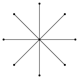
Figure 4: $K_{1,8}$ as an example of a star graph.

The eigenvalues of $\Delta(K_{1,N})$ are known as

$$\lambda_{0}=0\,,\quad\lambda_{p}=1\quad(p=1,2,\ldots,N-1)\,,\quad\lambda_{N}=N+1.$$ (67)

The determinant of $H=\Delta(K_{1,N})+l^{2}I_{N+1}$ is

$$\det H=D(0)=l^{2}\left(1+\frac{N}{1+l^{2}}\right)\left(1+l^{2}\right)^{N}\,.$$ (68)

6 Free energy on a graph

In this section, we consider applications of the results on determinants for studying discrete systems.

We first consider $N$ scalar degrees of freedom and define the action as follows:

$$S=\frac{1}{2}\left(\frac{N^{2}}{L^{2}}\sum_{k=1}^{N}\sum_{k^{\prime}=1}^{N}\phi_{k}\Delta(C_{N})_{kk^{\prime}}\phi_{k^{\prime}}+\mu^{2}\sum_{k=1}^{N}\phi_{k}^{2}\right)\,,$$ (69)

where $\Delta(C_{N})$ is the graph Laplacian for $C_{N}$ and

$$\mu\equiv\frac{2N}{L}\sinh\frac{mL}{2N}\,,$$ (70)

where $L$ and $m$ are constants.

Then, the Gaussian free energy on $C_{N}$ [26] is obtained using Eq. (42) as

$$F_{C_{N}}=\frac{1}{2}\ln\left[\det\left(\Delta(C_{N})+4\sinh^{2}\frac{mL}{2N}I_{N}\right)\right]=\ln\left(2\sinh\frac{mL}{2}\right)+const.\,.$$ (71)

This is interesting because the action (69) can be rewritten as

$$S=\frac{1}{2}\left[\frac{N^{2}}{L^{2}}\sum_{k=1}^{N}(\phi_{k}-\phi_{k+1})^{2}+\mu^{2}\sum_{k=1}^{N}\phi_{k}^{2}\right]\,,$$ (72)

under the ‘periodic’ condition, $\phi_{N+1}\equiv\phi_{1}$. A continuum limit, $a_{0}\equiv L/N\rightarrow 0$, enforces $\frac{\phi_{k+1}-\phi_{k}}{a_{0}}\rightarrow\partial_{x}\phi$, where $x$ is a coordinate of one dimension with periodicity $x+L\sim x$. Therefore, we can find that the one-loop free energy of a real scalar field $\phi(x)$ with mass $m$ on a circle ($S_{1}$) with circumference $L$ governed by the action

$$S=\frac{1}{2}\int dx\left[(\partial_{x}\phi)^{2}+m^{2}\phi^{2}\right]\,$$ (73)

takes the form

$$F_{S_{1}}=\ln\left(2\sinh\frac{mL}{2}\right)\,,$$ (74)

after some regularization [26, 27]. Note that since

$$2\sinh\frac{mL}{2}=mL\frac{\prod_{n=1}^{\infty}\left(\frac{4\pi^{2}n^{2}}{L^{2}}+m^{2}\right)}{\prod_{n=1}^{\infty}\left(\frac{4\pi^{2}n^{2}}{L^{2}}\right)}\,,$$ (75)

we find that the eigenvalues of $-\partial_{x}^{2}+m^{2}$, where $-\partial_{x}^{2}$ is the one-dimensional Laplacian on $S_{1}$, are shown by

$$\frac{4\pi^{2}n^{2}}{L^{2}}+m^{2}\quad(n\mbox{ is an integer})\,.$$ (76)

Similarly, we can consider the other matrices. For example, the action for complex scalar fields defined as

$$S = \frac{1}{2}\left(\frac{N^{2}}{L^{2}}\sum_{k=1}^{N}\sum_{k^{\prime}=1}^{N}\phi^{\dagger}_{k}{\Delta(C_{N},\chi)}_{kk^{\prime}}\phi_{k^{\prime}}+\mu^{2}\sum_{k=1}^{N}|\phi_{k}|^{2}\right)$$ (77)

$$= \frac{1}{2}\left[\frac{N^{2}}{L^{2}}\sum_{k=1}^{N}|\phi_{k}-e^{i\chi}\phi_{k+1}|^{2}+\mu^{2}\sum_{k=1}^{N}|\phi_{k}|^{2}\right]\,,$$

leads to the free energy

$$F_{C_{N},\chi} = \ln\left[\det\left(\Delta(C_{N},\chi)+4\sinh^{2}\frac{mL}{2N}I_{N}\right)\right]$$ (78)

$$= \ln\left(4\sinh^{2}\frac{Nz}{2}+4\sin^{2}\frac{N\chi}{2}\right)+const.\,.$$

Here we will avoid repeated discussion, and only note that the eigenvalue spectrum of the continuum limit of this case is given by

$$\frac{(2\pi n-\chi)^{2}}{L^{2}}+m^{2}\quad(n\mbox{ is an integer})\,.$$ (79)

Continuum limits exist also in other some cases.

The large $N$ limit of the determinant of $\Delta_{DD}+\mu^{2}I_{N}$ (according to Eq. (22)) becomes

$$\frac{\sinh mL}{\sinh\frac{mL}{N}}\rightarrow N\frac{\sinh mL}{{mL}}\,,$$ (80)

which coincides with the result of the example stated in Sec. 2 up to the constant. We find that the continuum limit corresponds to the system of massive scalar field in a line $0\leq x\leq L$ with Dirichlet-Dirichlet boundary conditions at its ends.

The large $N$ limit of the determinant of $\Delta_{DN}+\mu^{2}I_{N}$ (according to Eq. (25)) becomes simply

$$\cosh mL+2\sinh\frac{mL}{N}\sinh mL\rightarrow\cosh mL\,.$$ (81)

A comparison to a known mathematical relation

$$\cosh mL=\frac{\prod_{n=0}^{\infty}\left[\frac{\pi^{2}}{L^{2}}\left(n+\frac{1}{2}\right)^{2}+m^{2}\right]}{\prod_{n=0}^{\infty}\left[\frac{\pi^{2}}{L^{2}}\left(n+\frac{1}{2}\right)^{2}\right]}$$ (82)

leads to the conclusion that the continuum limit of spectrum is given by $\frac{\pi^{2}}{L^{2}}\left(n+\frac{1}{2}\right)^{2}+m^{2}$, thus the boundary conditions of the system is Dirichlet-Neumann condition.

Finally, the determinant of $\Delta(P_{N})+\mu^{2}I_{N}$ (according to Eq. (28)) is

$$2\tanh\frac{mL}{2N}\sinh mL\,.$$ (83)

Since the free energy is proportional to the logarhithm of this, we drop the $N$ dependent term (which is log divergent if $N\rightarrow\infty$). The boundary conditions of the continuum system is Neumann-Neumann condition (which can be judged from the existence of a zero mode).

In the next section, we will consider the way to obtain one-loop vacuum energy of scalar field theory with mass matrix required by structure of a theory space with four dimensional spacetime.

7 Vacuum energy from a theory space

7.1 formulation

One-loop vacuum energy density in quantum field theory can be derived from the functional determinants [2]. In the present paper, we only consider scalar field theories for simplicity. As seen in the previous section, $N$-scalar field theory can resemble compactification of a dimension. This is the key idea of the dimensional deconstruction [8, 9, 10]. The structure of the theory space is determined by the quadratic term of fields, i.e., the mass matrix. Suppose that a mass matrix (precisely, the $(mass)^{2}$ matrix) $\Delta/a_{0}^{2}$ is given (in other words, a theory space is given). The eigenvalues of $\Delta$ are denoted by $\lambda_{p}$, as previously. Then, using the characteristic polynomial $D(\lambda)=\prod_{p}(\lambda_{p}-\lambda)$, one-loop vacuum energy density for real scalar fields is calculated by

$$V=\frac{1}{2}\int\frac{d^{4}l}{(2\pi)^{4}}\ln\frac{\det[\Delta/a_{0}^{2}+l^{2}]}{\det[\Delta/a_{0}^{2}+l^{2}+M^{2}]}=\frac{1}{2a_{0}^{4}}(2\pi^{2})\int_{0}^{\infty}\frac{l^{3}dl}{(2\pi)^{4}}\ln\frac{D(-l^{2})}{D(-l^{2}-M^{2}a_{0}^{2})}\,,$$ (84)

where we used $M$ of the Pauli-Villars regularization, which is considered to be $M\rightarrow\infty$. The constant $a_{0}$ illustrates an overall scale in the theory space, i.e., related to mass scale of new physics via $a_{0}\sim m_{new~{}physics}^{-1}$.

In practice, regularization is an art of assembly of mathematical techniques. We adopt here the following approach. A physical value of the vacuum energy should be determined independently of the unphysical $M$ and the UV divergence must be subtracted in the expression of it. Thus, we consider, in the denominator in log in Eq. (84), as

$$D(-l^{2}-M^{2}a_{0}^{2})\Rightarrow\mbox{Asymptotic form of }D(-l^{2})\mbox{ when }l^{2}\rightarrow\infty\,.$$ (85)

Further, if the theory contains the $N$ (scalar) fields, the integrand of the most divergent part should be proportional to $N$. Thus, we extract the part of $\propto(l^{2})^{N}\subset D(-l^{2})$ for large $l^{2}$.

7.2 dimensional deconstruction of a circle

A concrete example is in order. We consider a theory space associated with $\Delta(C_{N},\chi)$. This model has widely been studied by many authors [8, 9, 10, 28]. We have already obtained $\det\left[\Delta(C_{N},\chi)+4\sinh^{2}\frac{z}{2}\,I_{N}\right]$ ($\propto D(-l^{2})$, in the present case) in Eq. (45). The asymptotic behavior can be found as

$$\det\left[\Delta(C_{N},\chi)+4\sinh^{2}\frac{z}{2}\,I_{N}\right]$$ (86)

$$= \left|e^{N(z+i\chi)/2}-e^{-N(z+i\chi)/2}\right|^{2}\rightarrow\left|e^{N(z+i\chi)/2}\right|^{2}(=e^{Nz})\quad(z\rightarrow\infty).$$

Thus, in our regularization scheme,

$$V(\chi)=\frac{1}{a_{0}^{4}}(2\pi^{2})\int_{0}^{\infty}\frac{dz}{(2\pi)^{4}}8\sinh^{3}\frac{z}{2}\cosh\frac{z}{2}\ln\frac{\left|e^{N(z+i\chi)/2}-e^{-N(z+i\chi)/2}\right|^{2}}{\left|e^{N(z+i\chi)/2}\right|^{2}}\,,$$ (87)

where we set $l=2\sinh\frac{z}{2}$. Now, the integration can be done by elementary methods as

$$V(\chi) = \frac{2\pi^{2}}{a_{0}^{4}}\int_{0}^{\infty}\frac{dz}{(2\pi)^{4}}4\sinh^{2}\frac{z}{2}\sinh z\left[\ln\left(1-e^{-N(z+i\chi)}\right)+\ln\left(1-e^{-N(z-i\chi)}\right)\right]$$ (88)

$$= -\frac{1}{16\pi^{2}a_{0}^{4}}\sum_{n=1}^{\infty}\int_{0}^{\infty}dz(e^{\frac{z}{2}}-e^{-\frac{z}{2}})^{2}(e^{z}-e^{-z})\left[\frac{e^{-Nn(z+i\chi)}}{n}+\frac{e^{-Nn(z-i\chi)}}{n}\right]$$

$$= -\frac{1}{8\pi^{2}a_{0}^{4}}\sum_{n=1}^{\infty}\frac{\cos Nn\chi}{n}\int_{0}^{\infty}dz(e^{2z}-2e^{z}+2e^{-z}-e^{-2z})e^{-Nnz}$$

$$= -\frac{1}{8\pi^{2}a_{0}^{4}}\sum_{n=1}^{\infty}\frac{\cos Nn\chi}{n}\left(\frac{1}{Nn-2}-\frac{2}{Nn-1}+\frac{2}{Nn+1}-\frac{1}{Nn+2}\right)$$

$$= -\frac{1}{8\pi^{2}a_{0}^{4}}\sum_{n=1}^{\infty}\frac{\cos Nn\chi}{n}\left(\frac{4}{N^{2}n^{2}-4}-\frac{4}{N^{2}n^{2}-1}\right)$$

$$= -\frac{3}{2\pi^{2}a_{0}^{4}}\sum_{n=1}^{\infty}\frac{\cos Nn\chi}{n(N^{2}n^{2}-1)(N^{2}n^{2}-4)}\,.$$

This result exactly coincides with the known result [8, 9, 10, 28]. Incidentally, for large $N$,

$$V(\chi)\sim-\frac{3}{2\pi^{2}(Na_{0})^{4}}\sum_{n=1}^{\infty}\frac{\cos Nn\chi}{n^{5}}\,,\quad V(0)\sim-\frac{3\zeta(5)}{2\pi^{2}(Na_{0})^{4}}\,,$$ (89)

where $\zeta(z)$ is the Riemann’s zeta function. We find that there exists a “continuum limit”, $N\rightarrow\infty$ as $Na_{0}$ and $N\chi$ are fixed.

7.3 the clockwork theory

Next, we turn to consider the theory space of the clockwork theory [20, 21, 22, 23] for real scalar fields. The action is

$$S=\frac{1}{2}\int d^{4}x\left[\sum_{k=1}^{N}(\partial_{\mu}\phi_{k})^{2}+m^{2}\sum_{k=1}^{N-1}(\phi_{k}-q\phi_{k+1})^{2}\right]\,,$$ (90)

where $m=a_{0}^{-1}$. Thus, the relevant matrix determinant is given as Eq. (31). The subtraction of UV divergence is subtle because of the complicated form of the determinant in this case. We separate the vacuum energy density into three parts, such as $V=V_{N}(q)+V_{0}+NV_{1}$. Here, $V_{N}(q)$ is a finite part ,

$$V_{N}(q)=\frac{1}{2a_{0}^{4}}(2\pi^{2})\int_{0}^{\infty}\frac{l^{3}dl}{(2\pi)^{4}}\ln\left[1-\left(\frac{\gamma_{-}}{\gamma_{+}}\right)^{N}\right]\,,$$ (91)

where $\gamma_{\pm}$ is given by Eq. (32). This will be of order of $O(N^{-4})$ as in the previous case and thus will have a continuum limit in vacuum energy density.

The change of the integration variable $\cosh y=\frac{\l^{2}+1+q^{2}}{2q}$ makes the integration simple. Then, we can rewrite $V_{N}(q)$ as

$$V_{N}(q)=\frac{1}{2a_{0}^{4}}(2\pi^{2})\int_{|\ln q|}^{\infty}\frac{dy}{(2\pi)^{4}}q\sinh y(2q\cosh y-1-q^{2})\ln\left(1-e^{-2Ny}\right)\,,$$ (92)

and we get the form with infinite summations,

$$V_{N}(q) = -\frac{q^{2}}{16\pi^{2}a_{0}^{4}}\sum_{n=1}^{\infty}\frac{q^{-2Nn}}{2n}\left[\frac{q^{2}}{(2Nn-2)(2Nn-1)}\right.$$ (93)

$$\qquad\left.-2\frac{1}{(2Nn-1)(2Nn+1)}+\frac{q^{-2}}{(2Nn+1)(2Nn+2)}\right]\quad(q\geq 1)\,,$$

$$V_{N}(q) = -\frac{q^{2}}{16\pi^{2}a_{0}^{4}}\sum_{n=1}^{\infty}\frac{q^{2Nn}}{2n}\left[\frac{q^{-2}}{(2Nn-2)(2Nn-1)}\right.$$ (94)

$$\qquad\left.-2\frac{1}{(2Nn-1)(2Nn+1)}+\frac{q^{2}}{(2Nn+1)(2Nn+2)}\right]\quad(q<1)\,.$$

Note that $q^{-2}V_{N}(q)=q^{2}V_{N}(q^{-1})$.

Figure 5: The numerical results for $(Na_{0})^{4}q^{-2(5/N)}V_{N}(q^{5/N})$ as functions of $q$ for $N=3,4,\ldots,10$, from lower to upper curves.

The numerical results for $(Na_{0})^{4}q^{-2(5/N)}V_{N}(q^{5/N})$ are shown in FIG. 5 for $N=3,4,\ldots,10$. These curves indicate that there is a continuum limit $N\rightarrow\infty$, while $Na_{0}$ and $q^{1/N}$ are fixed constants. If we can treat $q$ as a dynamical variable, the effective potential of $q$ seems to have a minimum at $q\sim 1$ for large $N$, where the mass matrix simply becomes the graph Laplacian of $P_{N}$. Note also that $V_{N}(q)\rightarrow 0$ both for $q\rightarrow 0$ and for $q\rightarrow\infty$.

We now estimate the separated contributions. They are written as

$$V_{0}=\frac{1}{2a_{0}^{4}}(2\pi^{2})\int_{0}^{\infty}\frac{l^{3}dl}{(2\pi)^{4}}\ln\frac{l^{2}}{\sqrt{(1-q^{2})^{2}+2(1+q^{2})l^{2}+l^{4}}}\,,$$ (95)

and

$$V_{1} = \frac{1}{2a_{0}^{4}}(2\pi^{2})\int_{0}^{\infty}\frac{l^{3}dl}{(2\pi)^{4}}\,\ln\gamma_{+}$$ (96)

$$= \frac{1}{2a_{0}^{4}}(2\pi^{2})\int_{0}^{\infty}\frac{l^{3}dl}{(2\pi)^{4}}\ln\left[\frac{1+q^{2}+l^{2}+\sqrt{(1-q^{2})^{2}+2(1+q^{2})l^{2}+l^{4}}}{2}\right]\,.$$

As for $V_{0}$, if we use the standard formula of derivation of the Coleman-Weinberg potential

$$\left.\frac{1}{2}\int\frac{d^{4}l}{(2\pi)^{4}}\ln(l^{2}+M^{2})\right|_{regularized}=\frac{M^{4}}{64\pi^{2}}\ln M^{2}\,,$$ (97)

to regularize $V_{0}$, aside from the contribution of a zero mode (as $\ln l^{2}$ in the integrand), we find

$$V_{0}=-\frac{1}{2(64\pi^{2})a_{0}^{4}}[(1-q)^{4}\ln(1-q)^{2}+(1+q)^{4}\ln(1+q)^{2}]\,.$$ (98)

It is notable that this contribution is equivalent to subtraction of the half of vacuum energy densities due to scalar fields with mass squared $(1-q)^{2}/a_{0}^{2}$ and $(1+q)^{2}/a_{0}^{2}$. The UV divergence of this part can be regarded to be canceled by the zero-mode contribution.

On the other hand, for the complicated form of a genuine divergent contribution of $NV_{1}$, we introduce a cut-off $\Lambda$ in the integration over $l$ and find

$$NV_{1} = \frac{N}{64\pi^{2}a_{0}^{4}}\left[\Lambda^{4}\left(\ln\Lambda^{2}-\frac{1}{2}\right)+2(1+q^{2})\Lambda^{2}-(1+4q^{2}+q^{4})\ln\frac{2\Lambda^{2}}{1+q^{2}+|1-q^{2}|}\right.$$ (99)

$$\left.+(1+q^{2})^{2}-\frac{3}{2}(1+q^{2})|1-q^{2}|\right]\,.$$

The quartic divergence seems to be independent of the structure of the mass matrix and the quadratic divergence is proportional to the trace of the mass matrix.

7.4 latticization of a disk

The matrix $\Delta(r,s)$ is used in [24, 25] as a latticization of a disk. Using the result of Eqs. (62) and (63), one-loop vacuum energy density of scalar field theory with mass matrix $\Delta(r,s)/a_{0}^{2}$ can be written formally as

$$V=\frac{2\pi^{2}}{2a_{0}^{4}}\int_{0}^{\infty}\frac{l^{3}dl}{(2\pi)^{4}}\ln\left[l^{2}\left(1+\frac{Ns}{s+l^{2}}\right)\left(\eta_{+}^{N}+\eta_{-}^{N}-2r^{N}\right)\right]$$

$$=V_{N}(r,s)+V_{0}+NV_{1}\,,$$ (100)

where

$$V_{N} = \frac{2\pi^{2}}{2a_{0}^{4}}\int_{0}^{\infty}\frac{l^{3}dl}{(2\pi)^{4}}\ln\left[1+\left(\frac{\eta_{-}}{\eta_{+}}\right)^{N}-2\left(\frac{r}{\eta_{+}}\right)^{N}\right]$$ (101)

$$= \frac{2\pi^{2}}{2a_{0}^{4}}\int_{0}^{\infty}\frac{l^{3}dl}{(2\pi)^{4}}\,2\ln\left[1-\left(\frac{r}{\eta_{+}}\right)^{N}\right]\,,$$

with

$$\eta_{+}\equiv\frac{1}{2}\left[2r+s+l^{2}+\sqrt{\left(2r+s+l^{2}\right)^{2}-4r^{2}}\right]\,,$$ (102)

$$V_{0}=\frac{2\pi^{2}}{2a_{0}^{4}}\int_{0}^{\infty}\frac{l^{3}dl}{(2\pi)^{4}}\ln\left[l^{2}\left(1+\frac{Ns}{s+l^{2}}\right)\right]\,,$$ (103)

and

$$V_{1} = \frac{2\pi^{2}}{2a_{0}^{4}}\int_{0}^{\infty}\frac{l^{3}dl}{(2\pi)^{4}}\ln\eta_{+}$$ (104)

$$= \frac{2\pi^{2}}{2a_{0}^{4}}\int_{0}^{\infty}\frac{l^{3}dl}{(2\pi)^{4}}\ln\frac{2r+s+l^{2}+\sqrt{\left(2r+s+l^{2}\right)^{2}-4r^{2}}}{2}\,.$$

A finite part $V_{N}$ can be rewritten as

$$V_{N}(s/r)=\frac{4\pi^{2}r^{2}}{2a_{0}^{4}}\int_{0}^{\infty}\frac{l^{3}dl}{(2\pi)^{4}}\,\ln\left[1-\left(\frac{2}{2+s/r+l^{2}+\sqrt{\left(2+s/r+l^{2}\right)^{2}-4}}\right)^{N}\right]\,.$$ (105)

Furthermore, introducing new variables $s/r=2\sin^{2}\frac{u}{2}$ and $\cosh y=l^{2}/2+\cosh u$, we find

$$V_{N}(u) = \frac{4\pi^{2}r^{2}}{2a_{0}^{4}}\int_{u}^{\infty}\frac{dy}{(2\pi)^{4}}\,2\sinh y(\cosh y-\cosh u)\ln\left[1-e^{-Ny}\right]$$ (106)

$$= -\frac{r^{2}}{8\pi^{2}a_{0}^{4}}\sum_{n=1}^{\infty}\frac{e^{-Nnu}}{n}\left[\frac{e^{2u}}{(Nn-2)(Nn-1)}\right.$$

$$\qquad\left.-2\frac{1}{(Nn-1)(Nn+1)}+\frac{e^{-2u}}{(Nn+1)(Nn+2)}\right]\,.$$

The numerical result of $(Na_{0})^{4}r^{-2}V_{N}(u/N)$ is plotted as a function of $N$ and $u$ in FIG. 6, where we treat $N$ as a continuous parameter.

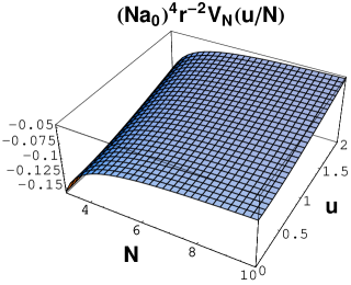
Figure 6: The numerical results for $(Na_{0})^{4}r^{-2}V_{N}(u/N)$ as a function of $N$ and $u$.

We find that $\lim_{N\rightarrow\infty}(Na_{0})^{4}r^{-2}V_{N}(0)=-\frac{3\zeta(5)}{4\pi^{2}}$, while we find no other limiting case for general $r$ and $s$, i.e., no precise continuum limit exists in general cases.

We now turn to consider the other part of the vacuum energy. For $V_{0}$, using similar estimation as in the previous subsection, we obtain, up to the zero-mode contribution,

$$V_{0}=\frac{1}{64\pi^{2}a_{0}^{4}}s^{2}\Bigl{\{}(N+1)^{2}\ln[(N+1)^{2}s^{2}]-\ln s^{2}\Bigr{\}}\,,$$ (107)

which is equivalent to the contribution of a scalar field with mass squared $(N+1)^{2}s^{2}/a_{0}^{2}$ minus the contribution of a scalar field with mass squared $s^{2}/a_{0}^{2}$. The UV divergence is canceled in this two contributions.

The divergent part is analyzed by using the cut-off $\Lambda$ and is found to be

$$NV_{1} = \frac{N}{64\pi^{2}a_{0}^{4}}\left[\Lambda^{4}\left(\ln\Lambda^{2}-\frac{1}{2}\right)+2(2r+s)\Lambda^{2}-(6r^{2}+4rs+s^{2})\ln\frac{2\Lambda^{2}}{2r+s+\sqrt{s(4r+s)}}\right.$$ (108)

$$\left.+(2r+s)^{2}-\frac{3}{2}(2r+s)\sqrt{s(4r+s)}\right]\,.$$

Again, we find that the quartic divergence is independent of the mass matrix and the quadratic divergence is proportional to the trace of the mass matrix.

In the next section, we will exhibit one more example of calculation of one-loop vacuum energy density for a slightly complicated theory space.

8 Some other examples of vacuum energy

Using the additional formulas on determinants, we can further obtain determinants of various matrices. In this section, we show some other examples below.

8.1 adding an edge with a vertex to each vertex of a graph

Let $\Delta_{N}$ be an $N\times N$ Hermitian matrix and define a $2N\times 2N$ matrix $\Delta_{2N}$ as follows:

$$\Delta_{2N}\equiv\left(\begin{array}[]{cc}\Delta_{N}+I_{N}&-I_{N}\\ -I_{N}&I_{N}\end{array}\right)\,,$$ (109)

where $I_{N}$ is an $N$ dimensional identity marix. In particular, if $\Delta_{N}$ is the graph Laplacian of a graph $G$, $\Delta_{2N}$ is the graph Laplacian of the graph generated by adding an edge with a vertex to every vertices of $G$.

Then, the formula on deteminants

$$\det\left(\begin{array}[]{cc}A&B\\ C&D\end{array}\right)=\det(A-BD^{-1}C)\det(D)$$ (110)

tells us that

$$\det(\Delta_{2N}-\lambda I_{2N})=(1-\lambda)^{N}\det\left(\Delta_{N}-\frac{1-(1-\lambda)^{2}}{1-\lambda}I_{N}\right)\,.$$ (111)

Therefore, if $D_{N}(\lambda)\equiv\prod_{p=1}^{N}(\lambda_{p}-\lambda)=\det(\Delta_{N}-\lambda I_{N})$, where $\{\lambda_{p}\}$ are eigenvalues of $\Delta_{N}$, is known, $D_{2N}(\lambda)\equiv\det(\Delta_{2N}-\lambda I_{2N})$ is obtained as

$$D_{2N}(\lambda)=(1-\lambda)^{N}D_{N}\left(\frac{1-(1-\lambda)^{2}}{1-\lambda}\right)\,.$$ (112)

For example, we will calculate vacuum energy density of the scalar field theory with mass matrix $\Delta_{2N}/a_{0}^{2}$, where $\Delta_{2N}$ is generated from $\Delta_{N}=\Delta(C_{N})$, i.e., $\Delta_{2N}$ is the graph Laplacian of the graph shown in FIG. 7.

Figure 7: The graph generated by adding an edge with a vertex to every vertices of $C_{9}$.

In this case, after some manipulation, we get

$$D_{2N}(\lambda)=\alpha(\lambda)^{N}\left[1-\left(\frac{1-\lambda}{\alpha(\lambda)}\right)^{N}\right]^{2}\,,$$ (113)

where

$$\alpha(\lambda)\equiv\frac{\lambda^{2}-4\lambda+2+\sqrt{\lambda(\lambda^{3}-8\lambda^{2}+16\lambda-8)}}{2}\,.$$ (114)

Now, we can obtain the vacuum energy density in this theory by utilizing $\ln D_{2N}(-l^{2})$, as in the previous section. We separate the finite and divergent parts of vacuum energy density as

$$V_{N}=\frac{1}{2a_{0}^{4}}(2\pi^{2})\int_{0}^{\infty}\frac{l^{3}dl}{(2\pi)^{4}}2\ln\left[1-\left(\frac{1+l^{2}}{\alpha(-l^{2})}\right)^{N}\right]\,,$$ (115)

and

$$V_{1}=\frac{1}{2a_{0}^{4}}(2\pi^{2})\int_{0}^{\infty}\frac{l^{3}dl}{(2\pi)^{4}}\ln\alpha(-l^{2})\,.$$ (116)

Figure 8: The numerical value of $(Na_{0})^{4}V_{N}$ for the model in this subsection as a function of $N$. The dotted lines indicate $\frac{1}{4}(Na_{0})^{4}V_{N}$, where $V_{N}$ is the vacuum energy density in the real scalar theory whose mass matrix is $\Delta(C_{N})/a_{0}^{2}$, and the constant $-\frac{3\zeta(5)}{16\pi^{2}}$.

The numerical result of $(Na_{0})^{4}V_{N}$ in the present case is shown in FIG. 8, where $N$ is treated as a continuous parameter. In the limit of $N\rightarrow\infty$, $(Na_{0})^{4}V_{N}$ approches $-\frac{3\zeta(5)}{16\pi^{2}}$, which is quarter of the value of the large $N$ limit of $(Na_{0})^{4}V_{N}$ in the case of the real scalar theory based on the graph Laplacian $\Delta(C_{N})$. The divergent part $NV_{1}$ can be estimated, because $\alpha(-l^{2})\sim l^{4}$ for large $l$, as

$$NV_{1}=\frac{2N}{64\pi^{2}a_{0}^{4}}\Lambda^{4}\left(\ln\Lambda^{2}-\frac{1}{2}\right)+\frac{N\Lambda^{2}}{8\pi^{2}}+\cdots\,.$$ (117)

The leading term is proportional to the number of real scalar fields, as expected. The quadratic divergence is proportional to the trace of the mass matrix.

8.2 the graph Cartesian products $G\times P_{2}$

Let $\Delta_{N}$ be an $N\times N$ Hermitian matrix and define a $2N\times 2N$ matrix $\hat{\Delta}_{2N}$ as follows:

$$\hat{\Delta}_{2N}\equiv\left(\begin{array}[]{cc}\Delta_{N}+I_{N}&-I_{N}\\ -I_{N}&\Delta_{N}+I_{N}\end{array}\right)\,.$$ (118)

In particular, if $\Delta_{N}$ is the graph Laplacian of a graph $G$, $\hat{\Delta}_{2N}$ is the graph Laplacian of the graph Cartesian product $G\times P_{2}$.

Then, the use of the formula on deteminants

$$\det\left(\begin{array}[]{cc}A&B\\ C&D\end{array}\right)=\det(A-BD^{-1}C)\det(D)=\det(AD-BC)\,,$$ (119)

provided that $[C,D]=0$, leads to

$$\det(\hat{\Delta}_{2N}-\lambda I_{2N}) = \det\left([\Delta_{N}+(1-\lambda)I_{N}]^{2}-I_{N}\right)$$ (120)

$$= \det\left(\Delta_{N}-\lambda I_{N}\right)\cdot\det\left(\Delta_{N}+(2-\lambda)I_{N}\right)\,.$$

Therefore, if $D_{N}(\lambda)\equiv\prod_{p=1}^{N}(\lambda_{p}-\lambda)=\det(\Delta_{N}-\lambda I_{N})$, where $\{\lambda_{p}\}$ are eigenvalues of $\Delta_{N}$, is known, $\hat{D}_{2N}(\lambda)\equiv\det(\hat{\Delta}_{2N}-\lambda I_{2N})$ is obtained as

$$\hat{D}_{2N}(\lambda)=D_{N}(\lambda)D_{N}(\lambda-2)\,.$$ (121)

The vacuum energy density of the scalar field theory with mass matrix $\hat{\Delta}_{2N}/a_{0}^{2}$, where $\hat{\Delta}_{2N}$ is generated from $\Delta_{N}=\Delta(C_{N})$, i.e., $\hat{\Delta}_{2N}$ is the graph Laplacian of the graph Cartesian product $C_{N}\times P_{2}$, called as the prism graph $Y_{N}$. We show the graph $Y_{9}$ in FIG. 9.

Figure 9: The graph Cartesian product $C_{9}\times P_{2}$, or the prism graph $Y_{9}$.

We can obtain the vacuum energy density in this theory by utilizing $\ln\hat{D}_{2N}(-l^{2})$. We separate the finite and divergent parts of vacuum energy density as

$$V_{N} = \frac{1}{16\pi^{2}a_{0}^{4}}\int_{0}^{\infty}{l^{3}dl}\cdot 2\left\{\ln\left[1-\left(\frac{2}{2+l^{2}+\sqrt{(2+l^{2})^{2}-4}}\right)^{N}\right]\right.$$ (122)

$$\qquad\qquad\qquad\qquad\left.+\ln\left[1-\left(\frac{2}{4+l^{2}+\sqrt{(4+l^{2})^{2}-4}}\right)^{N}\right]\right\}\,,$$

and

$$V_{1}=\frac{1}{16\pi^{2}a_{0}^{4}}\int_{0}^{\infty}{l^{3}dl}\left[\ln\frac{2+l^{2}+\sqrt{(2+l^{2})^{2}-4}}{2}+\ln\frac{4+l^{2}+\sqrt{(4+l^{2})^{2}-4}}{2}\right]\,.$$ (123)

Figure 10: The numerical value of $(Na_{0})^{4}V_{N}$ for the model whose theory space is associated with $Y_{N}$ as a function of $N$. The dotted lines indicate $(Na_{0})^{4}V_{N}$, where $V_{N}$ is the vacuum energy density in the real scalar theory whose mass matrix is $\Delta(C_{N})/a_{0}^{2}$, and the constant $-\frac{3\zeta(5)}{4\pi^{2}}$.

The numerical result of $(Na_{0})^{4}V_{N}$ in the present case is shown in FIG. 10, where $N$ is treated as a continuous parameter. In the limit of $N\rightarrow\infty$, $(Na_{0})^{4}V_{N}$ approches the vacuum energy density of the model associated with $C_{N}$ and $-\frac{3\zeta(5)}{4\pi^{2}}$. The divergent part $NV_{1}$ can be estimated as

$$NV_{1}=\frac{2N}{64\pi^{2}a_{0}^{4}}\Lambda^{4}\left(\ln\Lambda^{2}-\frac{1}{2}\right)+\frac{3N\Lambda^{2}}{16\pi^{2}}+\cdots\,.$$ (124)

The leading term is proportional to the number of real scalar fields, as expected. The quadratic divergence is proportional to the trace of the mass matrix.

9 Conclusion

In the present paper, we showed the method of obtaining the determinant of repetitive tridiagonal matrices with concrete examples. The concept of the method is similar to the Gel’fand–Yaglom method of obtaining functional determinants for differential operators.

The repetitive matrices as mass matrices are widely considered in modern models in particle physics, in order to attack the hierarchy problem by adopting a theory space. We showed one-loop vacuum energies of such models can be evaluated by using the determinant of the mass matrices obtained by our method stated in earlier sections.

We have seen that there are not always genuine continuum limits in large $N$ for general theory spaces. In Sec. 7, we have also found that contributions of $V_{0}$ expressed in logarithmic functions remain in general. They can be compensated by addition of bosonic or fermionic free fields with appropriate mass in some cases.

In future work, we wish to study one-loop energy density in models of deconstructed warped (theory) space [29, 30, 31, 32, 33, 34]. Although it is difficult to evaluate the determinants in a closed form in such a model, calculation based on recurrence relations would be suitable for a computer. It is also interesting to investigate the recent model of deconstruction of torus with magnetic flux [35].

If we would like to deal with the matrices related with more complicated graphs or higher dimensional lattices, we confront other difficulties. The graph Laplacians of generic graphs cannot be expressed by tridiagonal matrices. Though, fortunately, it is known that arbitrary square matrices can be systematically tridiagonalized by the Householder method [38] (see also Refs. [39, 40]). Thus, in principle, our Gel’fand–Yaglom-type method can be applied to the matrix with the general graph structure.

Finally, we add a comment on exclusion of zero modes. Zero modes of operators which appear in quantum field theory have crucial meanings related with nonperturbative aspects of the theory (see for example, the first section of Ref. [14]). In our present paper, we considered mass terms in almost all examples and the cases with zero modes can be considered as the limit that the value of mass goes to zero. Because we considered the vacuum energies and their dependence on the parameters in this paper, the analysis is just sound. Moreover, it is known that, if a matrix is expressed as a graph Laplacian of a simple graph (as in each example in this paper), the matrix has a single zero modes. Therefore, further analysis on zero modes, if necessary, could be fulfilled appropriately.

Data availability

No data were used to support this study.

Conflicts of interest

The authors declare that there are no conflicts of interest regarding the publication of this paper.

References

- [1] I. M. Gel’fand and A. M. Yaglom, J. Math. Phys. 1 (1960) 48.
- [2] G. V. Dunne, J. Phys. A41 (2008) 304006.
- [3] S. Coleman, Aspects of Symmetry, (Cambridge University Press, Cambridge, 1988).
- [4] C. Ccapa Ttira, C. D. Fosco and F. D. Mazzitelli, J. Phys. A44 (2011) 465403.
- [5] C. D. Fosco and F. D. Mazzitelli, arXiv:1708.08730 [hep-th].
- [6] B. L. Altshuler, Phys. Rev. D95 (2017) 086001.
- [7] B. L. Altshuler, arXiv:1706.06286 [hep-th].
- [8] N. Arkani-Hamed, A. G. Cohen and H. Georgi, Phys. Rev. Lett. 86 (2001) 4757.
- [9] C. T. Hill, S. Pokorski and J. Wang, Phys. Rev. D64 (2001) 105005.
- [10] C. T. Hill and A. K. Leibovich, Phys. Rev. D66 (2002) 016006.
- [11] R. J. Wilson, Introduction to Graph Theory, 4th ed. (Longman, New York, 1997).
- [12] J. S. Dowker, J. Phys. A45 (2012) 215203.
- [13] A. Ossipov, J. Phys. A51 (2018) 495201.
- [14] G. M. Falco, A. A. Fedorenko and I. A. Gruzberg, J. Phys. A50 (2017) 485201.
- [15] J. Zinn-Justin, Phase Transitions and Renormalization Group, (Oxford University Press, Oxford, 2007).
- [16] B. Mohar, The Laplacian spectrum of graphs, in Graph Theory, Combinatorics, and Applications, Y. Alavi et al. eds. (Wiley, New York, 1991), p. 871.
- [17] B. Mohar, Discrete Math. 109 (1992) 171.
- [18] B. Mohar, Some applications of Laplace eigenvalues of graphs, in Graph Symmetry, Algebraic Methods, and Applications, G. Hahn and G. Sabidussi eds. (Kluwer, Dordrecht, 1997), p. 225.
- [19] R. Merris, Linear Algebra Appl. 197 (1994) 143.
- [20] K. Choi and S. H. Im, JHEP 1601 (2016) 149.
- [21] D. E. Kaplan and R. Rattazzi, Phys. Rev. D93 (2016) 085007.
- [22] G. F. Giudice and M. McCullough, JHEP 1702 (2017) 036.
- [23] M. Farina, D. Pappadopulo, F. Rompineve and A. Tesi, JHEP 1701 (2017) 095.
- [24] F. Bauer, M. Lindner and G. Seidl, JHEP 0405 (2004) 026.
- [25] F. Bauer, T. Hällgren and G. Seidl, Nucl. Phys. B781 (2007) 32.
- [26] N. Kan and K. Shiraishi, J. Phys. A51 (2018) 035203 (23pp).
- [27] A. Monin, Phys. Rev. D94 (2016) 085013.
- [28] N. Kan, K. Sakamoto and K. Shiraishi, Eur. Phys. J. C28 (2003) 425.
- [29] A. Falkowski and H.-D. Kim, JHEP 0208 (2002) 052.
- [30] H. Abe, T. Kobayashi, N. Maru and K. Yoshioka, Phys. Rev. D67 (2003) 045019.
- [31] A. Katz and Y. Shadmi, JHEP 0411 (2004) 060.
- [32] C. D. Carone, J. Erlich and B. Glover, JHEP 0510 (2005) 042.
- [33] L. Randall, M. D. Schwartz and S. Thambyahpillai, JHEP 0510 (2005) 110.
- [34] J. de Blas, A. Falkowski, M. Pérez-Victoria and S. Pokorski, JHEP 0608 (2006) 061.
- [35] Y. Tatsuta and A. Tomiya, arXiv:1703.05263 [hep-th].
- [36] Y. Cho, N. Kan and K. Shiraishi, Acta Phys. Pol. B35 (2004) 1597.
- [37] G. V. Dunne and K. Kirsten, J. Phys. A39 (2006) 11915.
- [38] A. S. Householder, J. ACM 5 (1958) 339.
- [39] C. Lanczos, J. Res. Nat. Bureau of Standards 45 (1950) 255.
- [40] W. Givens, J. Soc. Indust. Appl. Math. 6 (1958) 26.