MorphNet: Fast & Simple Resource-Constrained Structure Learning of Deep Networks

Abstract

We present MorphNet, an approach to automate the design of neural network structures. MorphNet iteratively shrinks and expands a network, shrinking via a resource-weighted sparsifying regularizer on activations and expanding via a uniform multiplicative factor on all layers. In contrast to previous approaches, our method is scalable to large networks, adaptable to specific resource constraints (e.g. the number of floating-point operations per inference), and capable of increasing the network’s performance. When applied to standard network architectures on a wide variety of datasets, our approach discovers novel structures in each domain, obtaining higher performance while respecting the resource constraint.

1 Introduction

The design of deep neural networks (DNNs) has often been more of an art than a science. Over multiple years, top world experts have incrementally improved the accuracies and speed at which DNNs perform their tasks, harnessing their creativity, intuition, experience, and above all - trial-and-error. Structure design in DNNs has thus become the new feature engineering. Automating this process is an active research field that is gaining significance as DNNs become more ubiquitous in a variety of applications and platforms.

One key approach towards automated architecture search involves sparsifying regularizers. Initially it was shown that applying L1 regularization on weight matrices can reduce the number of nonzero weights with little effect on the performance (e.g. accuracy or mean-average-precision) of the DNN [33, 4]. However, as DNNs started powering more and more industrial applications, practical constraints such as inference speed and power consumption became of increasing importance. Standard L1 regularization can prune individual connections (edges) in a neural network, but this form of sparsity is ill-suited to modern hardware accelerators and does not result in a speedup in practice. To induce better sparsification, more recent work has designed regularizers which target neurons (a.k.a. activations) rather than weights [18, 32, 2]. While these techniques have succeeded in reducing the number of parameters of a network, they do not target reduction of a particular resource (e.g., the number of floating point operations, or FLOPs, per inference). In fact, resource specificity of sparsifying regularizers remains an under explored area.

A more recent approach to neural network architecture design expands the scope of the problem from only shrinking a network to optimizing every aspect of the network structure. Works using this approach  [36, 31, 25, 17] rely on an auxiliary neural network to learn the art of neural network design from a large number of trial-and-error attempts. While these proposals have succeeded in achieving new state-of-the-art results on several datasets [25, 37], they have done so at the cost of an exorbitant number of trial-and-error attempts. These methods require months or years of GPU time to obtain a single architecture, and become prohibitively expensive as the networks and datasets grow in complexity and volume.

Figure 1: ResNet101 based models with similar performance (around $0.426$ MAP on JFT, see Section 5). A structure obtained by shrinking ResNet101 uniformly by a $\omega=0.5$ factor (left), and structures learned by MorphNet when targeting FLOPs (center) or model size (i.e., number of parameters; right). Rectangle width is proportional to the number of channels in the layer and residual blocks are denoted in gray. $7\times 7$, $3\times 3$, and $1\times 1$ convolutions are in purple, blue and green respectively. The purple bar at the bottom of each model is thus the input layer. Learned structures are markedly different from the human-designed model and from each other. The FLOP  regularizer primarily prunes the early, compute-heavy layers. It notably learns to remove whole layers to further reduce computational burden. By contrast, the model size regularizer focuses on removal of $3\times 3$ convolutions at the top layers as those are the most parameter-heavy.

Given these various research directions, automatic neural network architecture design is currently effective only under limited conditions and given knowledge of the right tool to use. In this paper, we hope to alleviate this issue. We present MorphNet, a simple and general technique for resource-constrained optimization of DNN architectures.

Our technique has three advantages: (1) it is scalable to large models and large datasets; (2) it can optimize a DNN structure targeting a specific resource, such as FLOPs per inference, while allowing the usage of untargeted resources, such as model size (number of parameters), to grow as needed; (3) it can learn a structure that improves performance while reducing the targeted resource usage.

We show the efficacy of MorphNet on a variety of datasets. As a testament to its scalability, we find that on the JFT dataset [13], a dataset of 350M images and 20K classes, our method achieves 2.1% improvement in evaluation MAP while maintaining the same number of FLOPs per inference. The resources required by our technique to achieve this improvement are only slightly greater than the resources required to train the model once.

As evidence of our method’s ability to learn network architecture, we show that on Inception-v2 [28], a network structure which has been hand-tuned by experts, our method finds an improved network architecture which leads to an increase of $1.1\%$ test accuracy on ImageNet, again maintaining the same number of FLOPs per instance.

Lastly, to show constraint targeting, we present the results of applying our technique to a number of additional datasets while targeting different constraints. Our method is able to find unique, improved structures for each constraint, showing the benefits of constraint-specific targeting (see Figure 1).

Overall, we find our method provides a much needed general, automated, and scalable solution to the problem of neural architecture design, a problem which is currently only solved by a combination of context-specific approaches and manual labor.

2 Related Work

The need for automatic procedures to selectively remove or add weights to a DNN has been a topic of research for several decades.

Optimal Brain Damage [19, 10] proposed pruning the weights of a fully trained DNN based on their contribution to the objective function. Since the DNN is fully trained, the contribution of each parameter may be approximated using the Hessian. In this and similar pruning algorithms, it is often beneficial to add a penalty term to the loss to encourage less necessary weights to decrease in norm. Traditionally, the penalty has taken the form of L2 regularization, equivalent to weight-decay [6]. Later work [33] proposed to use an L1 regularization, which is known to induce sparsity [29, 24], thus alleviating the need for sophisticated estimates of a parameter’s contribution to the loss. We use an L1 regularization in our method for the same reasons.

An issue common to many pruning and penalty-based procedures for inducing network sparsity is that the removal of weights after training and the penalty during training adversely affects the performance of the model. Previous work [9] has noted the benefits of a multi-step training process, first training to induce sparsity and subsequently training again using the newer structure. We utilize the same paradigm in our approach, also finding that training a newer structure from scratch benefits overall performance.

In this work we note that sparsity in DNNs is useful only when it corresponds to the removal of an entire neuron rather than a single connection. Previous work has made this point as well. Group LASSO [34] was introduced to solve this problem and has been previously applied to DNNs [18, 32, 2, 23]. The specific technique we use is based on an L1 penalty applied to the scale variables of batch normalization [16]. This technique was also discovered by a recent work [21] and similar ideas appear elsewhere [15]. However, these works do not target a specific resource or demonstrate any improvement in performance. Moreover, they largely neglect to compare to naïve DNN shrinking strategies, such as applying a uniform multiplier to all layer sizes, which is crucial given that they often study DNNs that are significantly over-parameterized.

Previous works on sparsifying DNNs have traditionally focused on reducing model size (i.e., each individual parameter is equally valuable) [4, 20, 35]. Recent years have revealed that more nuanced prioritization is needed. For example in mobile applications [14], reducing latency is also important. Our work is formulated in a general way, thus making it applicable to a wide variety of application-specific constraints. Our evaluation studies model size and FLOPs-based constraints. FLOPs-based constraints have been studied previously [22, 31, 17], although we believe our work is the first to tackle the issue via cleverly designed sparsifying regularizers.

Many of these previous works focus on reducing the size of a network using sparsification. Our work supersedes such research, going further to show that one may maintain the size (or FLOPs per inference) and gain an increase in performance by changing the structure of a neural network. Other methods to learn the structure of a neural network have been proposed, especially focusing on when and how to expand the size of a neural network [7, 3]. While these techniques may be incorporated in our method, we believe the simplicity of our proposed iterative process is important. Our method is easy to implement and thus quick to try.

Finally, our work is distinct from a school of methods that learn the network structure from a large amount of trial-and-error attempts. These methods use RL [36, 31] or genetic algorithms [25, 17] with the purpose of finding a network architecture which maximizes performance. We note that some of these works have begun to investigate resource-aware optimization rather than maximizing performance at all costs [31, 17, 38]. Still, the amount of computation necessary for these techniques makes them unfeasible on large datasets and large models. In contrast, our approach is extremely scalable, requiring only a small constant number (often 2) of automated trial-and-error attempts.

3 Background

In this work, we consider deep feed-forward neural networks, typically composed of a stack of convolutions, biases, fully-connected layers, and various pooling layers, and in which the output is a vector of scores. In the case of classification, the final vector contains one score per each class.

We number the parameterized layers of the DNN $L=1,\dots,M+1$. Each layer $L$ corresponds to a convolution or fully-connected layer and has an input width $I_{L}$ and output width $O_{L}$ associated with it. In the case of a convolutional layer, $I_{L},O_{L}$ correspond to the number of input and output channels, respectively, and $O_{L-1}=I_{L}$ for most networks without concatenating residual connections. We consider $L=M+1$ to be the last layer of the neural network. Thus $O_{M+1}$ is the size of the final output vector.

Since a fully-connected layer may be considered as a special case of a convolution, we will henceforth only consider convolutions. Thus for each layer $L=1,\dots,M+1$ we also associate input spatial dimensions $w_{L},x_{L}$, output spatial dimensions $y_{L},z_{L}$, and filter dimensions $f_{L},g_{L}$. The weight matrix associated with layer $L$ thus has dimensions $I_{L}\times O_{L}\times f_{L}\times g_{L}$ and maps a $w_{L}\times x_{L}\times I_{L}$ input to a $y_{L}\times z_{L}\times O_{L}$ output.

The neural network is trained to minimize a loss:

$$\min_{\theta}\mathcal{L}(\theta),$$ (1)

where $\theta$ is the collective parameters of the neural network and $\mathcal{L}$ is a loss measuring a combination of how well the neural network fits the data and any additional regularization terms (e.g., L2 regularization on weight matrices).

3.1 Problem Setup

We are interested in a procedure for automatically determining the design of a neural network to optimize performance under a constraint of limiting the consumption of a certain resource (e.g., FLOPs per inference). In the fully general case, this would entail determining the widths $I_{L},O_{L}$, the filter dimensions $f_{L},g_{L}$, the number of layers $M$, which layers are connected to which, etc. In this paper, we restrict the task of neural network design to only optimize over the output widths $O_{1:M}$ of all layers. Thus we assume that we have a seed network design $O_{1:M}^{\circ}$, which in addition to an initial set of output widths also gives the filter dimensions, network topology, and other design choices that are treated as fixed. In Section E we elaborate on how our method can be extended to optimize over these additional design choices. However, we found that restricting the optimization to only layer widths can be effective while maintaining simplicity.

In formal terms, assume we are given a seed network design $O_{1:M}^{\circ}$ and that the objective in Eq. (1) is a suitable proxy for the performance. Let the constraint be denoted by $\mathcal{F}(O_{1:M})\leq\zeta$ for $\mathcal{F}$ monotonically increasing in each dimension. In this paper, $\mathcal{F}$ is either the number of FLOPs per inference or the model size (i.e., number of parameters), although our method is generalizable to other constraints. We would like to find the optimal dimensions,

$$O_{1:M}^{*}=\underset{\mathcal{F}(O_{1:M})\leq\zeta}{\operatorname{argmin}}\min_{\theta}\mathcal{L}(\theta).$$ (2)

4 Method

We motivate our approach by first presenting a naïve solution to Eq. (2): the width multiplier. Let $\omega\cdot O_{1:M}=\{\lfloor\omega O_{1}\rfloor,\dots,\lfloor\omega O_{M}\rfloor\}$ for $\omega>0$. Observe that $\omega<1$ results in a shrunk network and $\omega>1$ results in an expanded network. The width multiplier (with $\omega<1$) was first introduced in the context of MobileNet [14]. To solve Eq. (2) one may perform the following process:

1. Find the largest $\omega$ such that $\mathcal{F}(\omega\cdot O_{1:M}^{\circ})\leq\zeta$.

2. Return $\omega\cdot O_{1:M}^{\circ}$.

In most cases the form of $\mathcal{F}$ allows for easily finding the optimal $\omega$. Thus, unlike other methods which require training a network to determine which components are more or less necessary, application of a width multiplier is essentially free. Despite its simplicity, in our evaluations we found this approach to often give good solutions, especially when $O_{1:M}^{\circ}$ is already a well-structured network. The approach suffers, however, with decreased quality of the initial network design.

Consider now an alternative, more sophisticated approach based on sparsifying regularizers. We may augment the objective (1) with a regularizer $\mathcal{G}(\theta)$ which induces sparsity in the neurons, putting greater cost on neurons which contribute more to $\mathcal{F}(O_{1:M})$. The trained parameters $\theta^{*}=\text{argmin}_{\theta}~{}\{\mathcal{L}(\theta)+\lambda\mathcal{G}(\theta)\}$ then induce a new set of output widths $O_{1:M}^{\prime}$ which are a tradeoff between optimizing the loss given by $\mathcal{L}$ and satisfying the constraint given by $\mathcal{F}$. Unlike the width multiplier approach, this approach is able to change the relative sizes of layers. However, the resulting structure $O_{1:M}^{\prime}$ is not guaranteed to satisfy $\mathcal{F}(O_{1:M}^{\prime})\leq\zeta$. Moreover, this procedure often disproportionately sacrifices performance, especially when $\mathcal{F}(O_{1:M}^{\prime})<\zeta$.

4.1 Our Approach

We propose to utilize a hybrid of the two approaches, iteratively alternating between a sparsifying regularizer and a uniform width multiplier. Given a suitable regularizer $\mathcal{G}$ which induces sparsity in the activations, putting greater cost on activations which contribute more to $\mathcal{F}(O_{1:M})$ (we elaborate on the specific form of $\mathcal{G}$ in subsequent sections), we propose to approximately solve Eq. (2) starting from the seed network $O_{1:M}^{\circ}$ using Algorithm 1.

The MorphNet algorithm optimizes the DNN by iteratively shrinking (Steps 1-2) and expanding (usually, Step 3) the DNN. At the shrinking stage, we apply a sparsifying regularizer on neurons. This results in a DNN that consumes less of the targeted resource, but typically achieves a lower performance. However, a key observation is that the training process in Step 1 not only highlights which layers of the DNN are over-parameterized, but also which layers are bottlenecked. For example, when targeting FLOPs, higher-resolution neurons in the lower layers of the DNN tend to be sacrificed more than lower-resolution neurons in the upper layers of the DNN. The situation is the exact opposite when the targeted resource is model size rather than FLOPs.

Algorithm 1 The MorphNet Algorithm

1:Train the network to find

2:$\theta^{*}=\underset{\theta}{\operatorname{argmin}}\{\mathcal{L}(\theta)+\lambda\mathcal{G}(\theta)\}$, for suitable $\lambda$.

3:Find the new widths $O_{1:M}^{\prime}$ induced by $\theta^{*}$.

4:Find the largests $\omega$ such that $\mathcal{F}(\omega\cdot O_{1:M}^{\prime})\leq\zeta$.

5:Repeat from Step 1 for as many times as desired, setting $O_{1:M}^{\circ}=\omega\cdot O_{1:M}^{\prime}$.

6:return $\omega\cdot O_{1:M}^{\prime}$.

This leads us to Step 3 of the MorphNet algorithm, which usually performs an expansion. In this paper we only report one method for expansion, namely uniformly expanding all layer sizes via a width multiplier as much as the constrained resource allows, although one may replace this with an alternative expansion technique.

We have thus completed one cycle of improving the network architecture, and we can continue this process iteratively until the performance is satisfactory, or until the DNN architecture has converged (i.e., further iterations lead to a near-identical DNN structure). In our evaluation below, we found a single iteration of Steps 1-3 to be enough to yield a noticeable improvement over the naïve technique of just using a uniform width multiplier, while subsequent iterations can bring additional benefits in performance. The optimal number of iterations, and whether the process converges, is yet to be investigated. Note that a single iteration of the MorphNet algorithm comes at the cost of a number of training runs equal to the number of values of $\lambda$ attempted, often a small constant number (i.e., 5 or less). Empirically, we found it easy to find a good range of $\lambda$ by trial-and-error. Whether a value is too large or too small is evident very early on in training by observing if the constrained quantity collapses to zero or does not decrease at all.

We use the remainder of this section to elaborate on the specifics of MorphNet. We begin by describing the calculation of $\mathcal{F}$ for the two constraints we consider (FLOPs and model size). We then describe how a penalty on this constraint may be relaxed to a simple yet surprisingly effective regularizer $\mathcal{G}$ with informative sub-gradients. Subsequently, we describe how to maintain the sparsifying nature of $\mathcal{G}$ when network topologies are not confined to the traditional paradigm of stacked layers with only local connections (i.e., as in Residual Networks). Extensions to MorphNet to make it applicable to design choices beyond just layer widths are briefly discussed in the supplementary material

4.2 Constraints

In this paper we restrict the discussion to two simple types of constraints: the number of FLOPs per inference, and the model size (i.e., number of parameters). However, our approach lends itself to generalizations to other constraints, provided that they can be modeled.

Both the FLOPs and model size are dominated by layers associated with matrix multiplications - i.e., convolutions. The FLOPs and model size are bilinear in the number of inputs and outputs of that layer:

$$\mathcal{F}(\text{layer }L)=C(w_{L},x_{L},y_{L},z_{L},f_{L},g_{L})\cdot I_{L}O_{L}.$$ (3)

In the case of a FLOPs constraint we have,

$$C(w,x,y,z,f,g)=2yzfg,$$ (4)

and in the case of a model size constraint we have,

$$C(w,x,y,z,f,g)=fg.$$ (5)

For ease of notation, we will henceforth drop the arguments from $C$ and assume them to be implicit. The constraints also include the relatively small cost of the biases, which is linear in $O_{L}$, and omitted here to avoid clutter.

A sparsifying regularizer on neurons will induce some of the neurons to be zeroed out. Namely, the weight matrix will exhibit structured sparsity in such a way that the pre-activation at some index $i$ is zero for any input and the post-activation at the same index is a constant. Such neurons should be discounted from Eq. (3) since an equivalent network may be constructed without the weights leading into and out of these neurons. To reflect this, we rewrite Eq. (3) as,

$$\mathcal{F}(\text{layer }L)=C\sum_{i=0}^{I_{L}-1}A_{L,i}\sum_{j=0}^{O_{L}-1}B_{L,j},$$ (6)

where $A_{L,i}$ ($B_{L,j}$) is an indicator function which equals one if the $i$-th input ($j$-th output) of layer $L$ is alive – not zeroed out. Eq. (6) represents an expression for the constrained quantity pertaining to a single convolution layer. The total constrained quantity is obtained by summing Eq. (6) over all layers in the DNN:

$$\mathcal{F}(O_{1:M})=\sum_{L=1}^{M+1}\mathcal{F}(\text{layer }L).$$ (7)

4.3 Regularization

When shrinking a network, we wish to minimize the loss of the DNN $\mathcal{L}(\theta)$ subject to a constraint $\mathcal{F}(O_{1:M})\leq\zeta$. The optimization problem is equivalent to applying a penalty on the loss,

$$\min_{\theta}\mathcal{L}(\theta)+\lambda\mathcal{F}(O_{1:M}),$$ (8)

for a suitable $\lambda$. Note that $\mathcal{F}$ is implicitly a function of $\theta$, since its calculation (Eq. (6) and Eq. (7)) relies on indicator functions. For tractable learning via gradient descent, it is necessary to replace the discontinuous L0 norm that appears in Eq. (6) with a continuous proxy norm. There are many possible choices for this continuous proxy norm.

In this work we choose to use an L1 norm on the $\gamma_{L}$ variables of batch normalization [16]. We chose this regularization because it is simple and widely applicable. Indeed, many top-performing feed-forward models apply batch normalization to each layer. This means that each neuron has a particular $\gamma$ associated with it which determines its scale. Setting this $\gamma$ to zero effectively zeros out the neuron.

Thus our relaxation of Eq. (6) is

$$\mathcal{G}(\theta,\text{layer }L)=C\sum_{i=0}^{I_{L}-1}|\gamma_{L-1,i}|\sum_{j=0}^{O_{L}-1}B_{L,j}+\\ C\sum_{i=0}^{I_{L}-1}A_{L,i}\sum_{j=0}^{O_{L}-1}|\gamma_{L,j}|,$$ (9)

where for ease of notation we assume the input neurons to layer $L$ are given by layer $L-1$. The regularizer for the whole network is then

$$\mathcal{G}(\theta)=\sum_{L=1}^{M+1}\mathcal{G}(\theta,\text{layer }L).$$ (10)

Note that the $A$ and $B$ coefficients in Eq. (9) are dynamic quantities, being piece-wise constant functions of the network weights. As neurons at the input of layer $L$ are zeroed out, the cost of each neuron at the output is reduced, and vice versa for neurons at the output of layer $L$. Eq. (9) captures this behavior. In particular, Eq. (9) is discontinuous with respect to the $\gamma$’s. However, Eq. (9) is still differentiable almost everywhere, and thus we found that standard minibatch optimizers readily handle the discontinuity of $\mathcal{G}$.

Figure 2: A histogram of $\gamma$ for one of the ResNet101 bottleneck layers when trained with a FLOP regularizer. Some of the $|\gamma|$’s are zeroed out, and are separated by a clear gap from the nonzero $|\gamma|$’s.

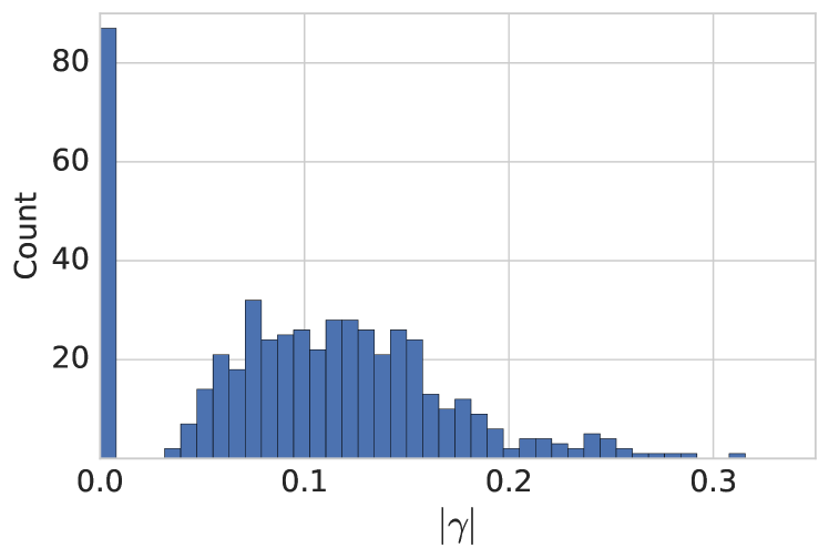
While our regularizer is simple and general, we found it to be surprisingly effective at inducing sparsity. We show the induced values of $\gamma$ for one network trained with $\mathcal{G}$ in Figure 2. There is a clear separation between those $\gamma$’s which have been zeroed out and those which continue to contribute to the network’s computation.

4.4 Preserving the Network Topology

DNNs in computer vision applications often have residual (skip) connections: i.e., the input of layer $L_{3}$ can be the sum of the outputs of $L_{1}$ and $L_{2}$. If the outputs of $L_{1}$ and $L_{2}$ are regularized separately, it is not guaranteed that the exact same outputs will be zeroed out in $L_{1}$ and $L_{2}$, which can change the topology of the network and introduce new types of connectivity that did not exist before. While the latter is a legitimate modification of the network structure, it may result in a significant complication in the network structure when the network has tens of layers tied to each other via residual connections. To avoid these changes in the network topology, we group all neurons that are tied in skip connections via a Group LASSO. For example, in the example above the $j$-th output of $L_{1}$ will be grouped with the $j$-th output of $L_{2}$. There are multiple ways to group them, and in the results presented in this work we use the $L_{\infty}$ norm - the maximum of the $|\gamma|$’s in the group.

5 Empirical Evaluation

We evaluate the MorphNet algorithm for automatic structure learning on a variety of datasets and seed network designs. We give a brief overview of each experimental setup in Section 5.1. In Section 5.2, we go through in detail the application of MorphNet on one of these setups (Inception V2 on ImageNet), examining the benefit and improvement at each step of the algorithm. We then give a summarized view of the results of MorphNet applied to all datasets and all models in Section 5.3. Finally, we take a closer look at our regularization in Section 5.4, showing that it adequately targets the desired constraint using both quantitative and qualitative analysis.

5.1 Datasets

We evaluate on a number of different datasets encompassing various scales and domains.

5.1.1 ImageNet

ImageNet [5] is a well-known benchmark consisting of 1M images classified into 1000 distinct classes. We apply MorphNet on two markedly different seed architectures: Inception V2 [28], and MobileNet [14]. These two networks were the result of hand-tuning to achieve two distinct goals. The former network was designed to have maximal accuracy (on ImageNet) while the latter was designed to have low computation foot-print (FLOPs) on mobile devices while maintaining good overall ImageNet accuracy.

For MobileNet we use the smallest published resolution ($128\times 128$) and the two smallest width multipliers ($50\%$ and $25\%$). We choose these as it focuses MorphNet on the low-FLOPs regime, thus furthest away from the Inception V2 regime.

5.1.2 JFT

At its introduction, ImageNet was significant for its size. Recent years have seen ever larger datasets. To evaluate the scalability of MorphNet, we choose the JFT dataset [13, 27], an especially large collection of labelled images, with about 350M images and about 20K labels. For this dataset we chose to start with the ResNet101 architecture [11], thus examining the applicability of MorphNet to residual networks.

5.1.3 AudioSet

Finally, as a dataset encompassing a different domain, we evaluate on AudioSet [8]. The published AudioSet contains $2$M audio segments encompassing $500$ distinct labels. We use a larger version of the dataset which contains $20$M labelled audio segments, while maintaining approximately the same number of labels. We seeded our model architecture with a residual network based on a structure previously used for this dataset [12].

5.2 A Case Study: Inception V2 on ImageNet

We provide a detailed look at each step of MorphNet (described in Section 4.1) on ImageNet with the seed network design $O_{1:M}^{\circ}$ corresponding to Inception V2 [28].

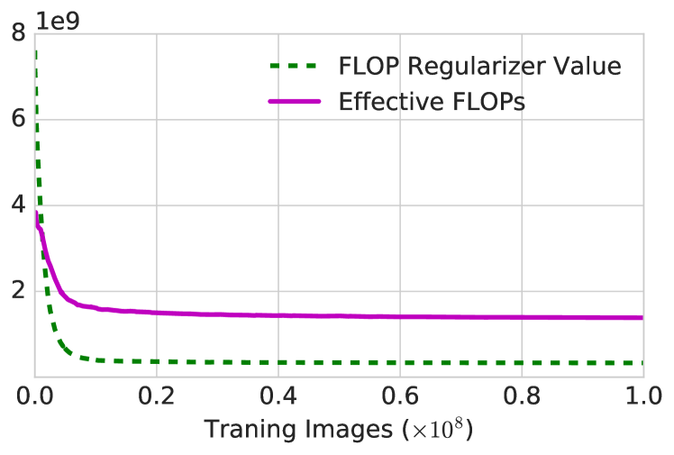
The shrinking stage of MorphNet trains the network with a sparsity-inducing regularizer $\mathcal{G}$. We use a FLOPs-based regularizer and show the effect of this regularizer on the actual FLOPs during training in Figure 3. Although the form of $\mathcal{G}$ is only a proxy to the true FLOPs, it is clear that the regularizer adequately targets the desired constraint.

Figure 3: Rapid convergence of of the FLOP regularization (green, dashed) and projected number of FLOPs (purple) for ImageNet trained with a FLOP regularizer strength of $\lambda=1.3\cdot 10^{-9}$. The projected number of FLOPs is computed by assuming all $|\gamma|<0.01$ are zeroed-out.

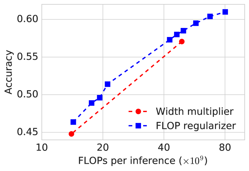
Applying $\mathcal{G}$ with different strengths (different values of $\lambda$) leads to different shrunk networks. We show the results of these distinct trained networks (blue line) compared to a naïve application of the width multiplier (red line) in Figure 4. While it is clear that sparsifying using $\mathcal{G}$ is more effective than applying a width multiplier, our main goal in this work is to demonstrate that the accuracy of the DNN can be improved while maintaining a constrained resource usage (FLOPs in this case).

Figure 4: ImageNet evaluation accuracy for various downsized versions of Inception V2 using both a naïve width multiplier (red circles) and a sparsifying FLOP regularizer (blue squares). We also show the result of re-expanding one of the networks induced by the FLOP regularizer to match the FLOP cost of the original network (pentagon point). A further increase in accuracy is achieved by performing the sparsifying and expanding process a second time (star point).

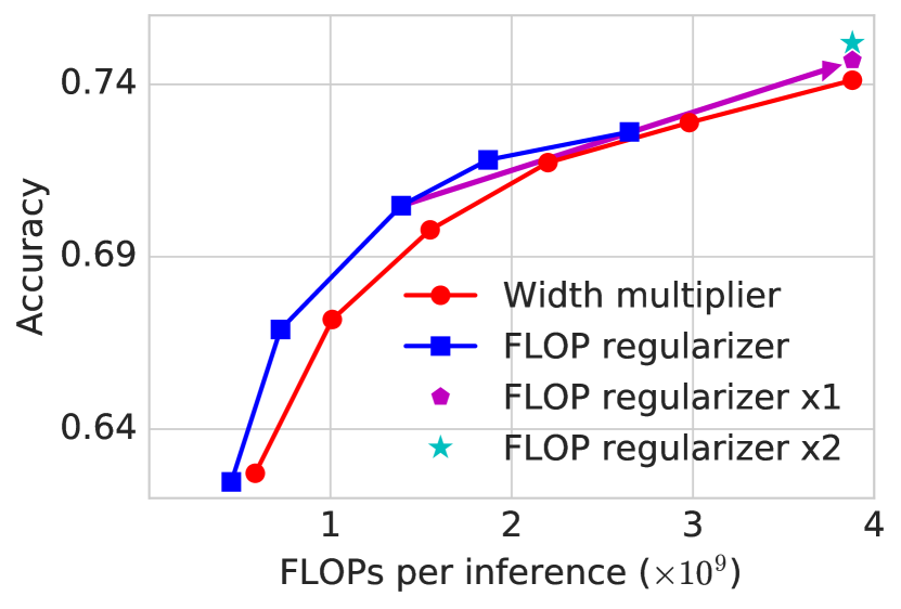
This leads us to MorphNet’ expansion stage (Step 3). We choose the DNN obtained by using $\lambda=1.3\cdot 10^{-9}$ to re-scale using a uniform width multiplier until the number of FLOPs per inference matches that of the seed Inception V2 architecture. See results in Figure 4 and Table 1. The resulting DNN achieves an improved accuracy compared to the Inception V2 baseline of 0.6%. We then repeat our procedure again, first applying a sparsifying regularizer and then re-scaling to the original FLOPs usage. On the second iteration we achieve a further improvement of 0.5%, adding up to a total improvement of 1.1% compared to the baseline. Since the improved DNN structures exhibited stronger overfitting than the seed, we introduced a dropout layer before the classifier (crucially, we were not able to improve the accuracy of the seed network in a significant manner by applying dropout). The dropout values and the accuracies are summarized in Table 1. Except for the dropout, all other hyperparameters used at training were identical for all DNNs.

In this case study we focused on improving accuracy while preserving the FLOPs per inference. However, it is clear that MorphNet can trade-off the two objectives when a practitioner’s priorities are different. For example, we found that the architecture learned in the second iteration can be shrunk by applying a width multiplier until the number of FLOPs is reduced by 30%, and the resulting DNN matches the original Inception V2 accuracy.

Iteration	$\omega$	Dropout	Weights	Accuracy
$0$	NA	0	$1.12\cdot 10^{7}$	74.1%
$1$	$1.69$	10%	$1.61\cdot 10^{7}$	74.7%
$2$	$1.57$	20%	$1.55\cdot 10^{7}$	75.2%

Table 1: MorphNet applied to the seed network of Inception V2 on ImageNet. A regularization strength of $\lambda=1.3\!\cdot\!10^{-9}$ was used in both iterations. The network was expanded to match the original FLOPs of $3.88\!\cdot\!10^{9}$. Dropout rate was increased to mitigate over-fit caused by the increased model capacity. Although the number of FLOPs is constant, our method is capable of and chooses to increase the number of weights in the model.

5.3 Improved Performance at No Cost

Network	Baseline	MorphNet	Relative Gain
Inception V2	74.1	75.2	+1.5%
MobileNet $50\%$	57.1	58.1	+1.78%
MobileNet $25\%$	44.8	45.9	+2.58%
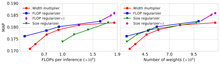
ResNet101	0.477	0.487	+2.1%
AudioResNet	0.182	0.186	+2.18%

Table 2: The result of applying MorphNet to a variety of datasets and model architectures while maintaining FLOP cost.

Figure 5: MAP vs. FLOPs (left) and MAP vs. model-size (right) curves on JFT (top) and AudioSet (bottom). The magenta points in the AudioSet figures represent models expanded from a FLOP (diamond) or size (pentagon) regularizes.

We present the collective results of MorphNet on all experimental setups on a FLOPs constraint in Table 2. In each setup we report the application of MorphNet to the seed network for a single iteration (two for Inception V2). Thus, each result requires up to three training runs.

We see improvements in performance across all datasets. The 1% improvement on MobileNet is especially impressive because MobileNet was specifically hand-designed to optimize accuracy under a FLOPs-constraint.

On JFT, an especially large dataset, we achieve over $2.1\%$ relative improvement. We note that the first training run is run until the convergence of the FLOPs cost, which is approximately 20 times faster than the convergence of the performance metric (MAP). Thus, for a given value of $\lambda$, a single iteration of MorphNet adds only 5% to the cost of training a single model. Since more than one attempt may be required to find a suitable $\lambda$, the actual added cost may be higher.

In AudioSet we continue to see the benefits of MorphNet, observing a 2.18% relative increase in MAP. To put this into perspective, an equivalent drop of 2.18% from the seed model corresponds to a FLOPs per inference reduction of over 50% (see Figure 5).

5.4 Resource Targeting

One of the contributions of this work is the form of the regularizer $\mathcal{G}$, which methodically targets a particular resource. In this section we demonstrate its effectiveness.

Figure 5 shows the results of applying a FLOPs-targeted $\mathcal{G}$ and a model size-targeted $\mathcal{G}$ at varying strengths. It is clear that the structures induced when targeting FLOPs form a better FLOPs/performance tradeoff curve, but poor model size/performance tradeoff curves, and vice versa when targeting model size.

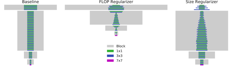
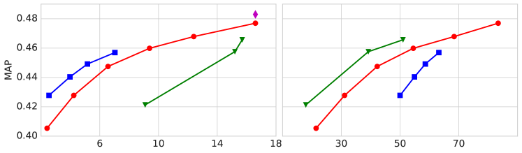
We may also examine the learned structures when targeting different resources. In Figure 1 we present the induced network structures when targeting FLOPs and when targeting model size. One thing to notice is that the FLOP regularizer tends to remove neurons from the lower layers near the input, whereas the model size regularizer tends to remove neurons from upper layers near the output. This makes sense, as the lower layers of the neural network are applied to a high-resolution image, and thus consume a large number of the total FLOPs. In contrast, the upper layers of a neural network are typically where the number of channels is higher and thus contain larger weight matrices. The two very different learned structures in Figure 1 achieve similar MAP (0.428 and 0.421, whereas the baseline model with similar cost is 0.405).

An interesting byproduct of applying MorphNet to residual networks is that the network also learns to shrink the number of layers, as shown in the FLOP regularized structure in Figure 1. When all the residual filters in a layer are pruned, the output is a direct copy of the input and the layer essentially can be removed. Therefore MorphNet achieves automatic layer shrinkage without any added complexity.

6 Conclusion

We presented MorphNet, a technique for learning DNN structures under a constrained resource. In our analysis of FLOP and model size constraints, we have shown that the form of the tradeoff between constraint and accuracy is highly dependent on the specific resource, and that MorphNet can successfully navigate this tradeoff when targeting either FLOPs or model size. Furthermore, we have applied MorphNet to large scale problems to achieve improvements over human-designed DNN structures, with little extra training cost compared to training the DNN once. While being highly effective, MorphNet is simple to implement and fast to apply, and thus we hope it becomes a general tool for machine learning practitioners aiming to better automate the task of neural network architecture design.

Appendix A Inception V2 trained on ImageNet

In this section we provide the technical details regarding the the experiments in Section 5.2 of the paper.

When training with a FLOP regularizer, we used a learning rate of $10^{-3}$, and we kept it constant in time. The values of $\lambda$ that were used to obtain the points displayed in Figure 4 are 0.7, 1.0, 1.3, 2.0 and 3.0, all times $10^{-9}$.

Tables 3 and 4 below lists the size of each convolution in Inception V2, for the seed network and for the two MorphNet iterations. The names of the layers are the ones generated by this code. Each column represents a learned DNN structure, obtained from the previous one by applying a FLOP regularizer with $\lambda=1.3\cdot 10^{-9}$ and then the width multiplier that was needed to restore the number of FLOPs to the initial value of $3.88\cdot 10^{9}$. The width multipliers at iteration 1 and 2 respectively were 1.692 and 1.571.

Appendix B MobileNet Training Details

B.1 Training protocol

Our models operate on $128\times 128$ images. The training procedure is a slight variant of running the main MorphNet algorithm for one iteration. This variability gives better results overall and is crucial for MorphNet to overtake the $50\%$ width-multipler model (see below). The procedure is as follows:

1. The full network (width-multipler of $1.0$ on $128\times 128$ image input) was first trained for $2$ million steps (which is the typical number of steps for a network’s performance to plateau as observed from training models with similar model sizes). Note that training smaller networks (e.g. with a width-multiplier of $0.25$) takes significantly more steps, e.g. around $10$ millions steps, to converge.

2. The checkpoint was used to initialize MorphNet training, which goes on for an additional $10$ million steps or until the FLOPs of the active channels converge, whichever is longer. We tried a range of $\lambda$ values $\in\{3,4,\ldots,10,11\}\times 10^{-9}$ to ensure that the converged FLOPs remain close to the FLOPs of the width-multiplier baselines.

3. We took the converged checkpoint and extracted a pruned network (both structure and weights) that consists of only the active channels.

4. Finally, we fine-tuned the pruned network using a small learning rate ($0.0013$). This is merely to restore moving average statistics for batch-normalization, and normally takes a negligible number, e.g. $20k$, of steps. While training for longer keeps improving the accuracy, simply training for $20k$ steps suffices to outperform models with width multipliers.

All training steps use the same optimizer, which is discussed below.

B.2 Trainer

We use the same trainer from MobileNet v2 [26], described below. We trained with the RMSProp optimizer [30] implemented in Tensorflow [1] with a batch-size of $96$. The initial learning rate was chosen from $\{0.013,0.045\}$, unless otherwise specified. The learning rate decays by a factor of $0.98$ every $2.5$ epochs. Training uses $16$ workers asynchronously.

B.3 Observations

Figure 6: ImageNet evaluation accuracy for various MobileNets on $128\times 128$ images using both a naïve  width multiplier (red circles) and a sparsifying FLOP regularizer (blue squares).

The total training time for each attempted $\lambda$ value is around $2+10=12$ million steps, which is less than twice the number of steps (around $10$ million) for training a regular network. Although multiple $\lambda$ values are required, each one of them contributes to the “optimal” FLOPs-vs-accuracy tradeoff, as shown in figure 6. The “optimality” is defined in a narrow sense that no model is dominated in both FLOP and accuracy by another. By contrast, the $50\%$ width-multipler model is dominated by the MorphNet models. Finally, we found that both the learning rate and the $\lambda$ parameter affects the converged FLOPs, but just the $\lambda$ parameter by itself suffices to traverse the range of desirable FLOPs.

Figure 7: Each of the four figures show the width of units in ResNet101 blocks (1-4). The green (blue) shaded lines represent different strength of the FLOP (size) regularizer. The purple line represents the unit width of a model expanded from a FLOP-regularized ResNet101 model so that the number of FLOPs matches these of the seed model. One can observe that increasing strengths of the FLOP regularizer (darker blue) remove more and more neurons from all blocks, and remove entire residual units (layers) from all blocks except for Block 4. Increasing the strength of the size regularizer (darker green) mainly removes neurons from Block 4.

Figure 8: A scatter plot of relative standard deviations v.s. average number of filters of each layer in ImageNet Inception V2 model. The standard deviation was calculated over the results of 10 independent runs of Inception V2 with a FLOP regularizer of $\lambda=1.3\cdot 10^{-9}$, using the same hyperparameter configuration.

Appendix C ResNet101 on JFT

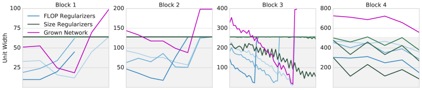
The FLOP regularizer $\lambda$-s used in Figure 5 on JFT were 0.7, 1.0, 1.3 and 2 times $10^{-9}$. The size regularizer $\lambda$-s were 0.7, 1 and 3 times $10^{-7}$. The width multiplier values were 1.0, 0.875, 0.75, 0.625, 0.5, and 0.375. Figure 7 illustrates the structures learned when applying these regularizers on ResNet101.

Appendix D Stability of MorphNet

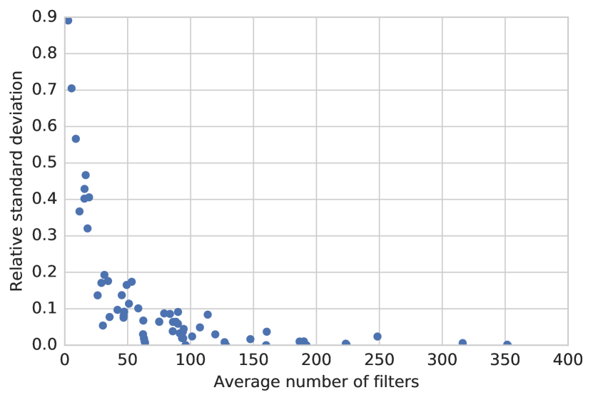
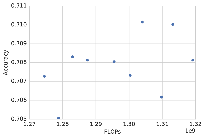
In this section, we study the stability of MorphNet with Inception V2 model on the ImageNet dataset. We trained the Inception V2 model regularized by FLOP regularizer with a constant learning rate of $10^{-3}$. We also set the value of $\lambda$ to be $1.3\times 10^{-9}$. The training procedure was repeated independently for 10 times. We extracted the final architecture, e.g. the number of filters in each layer, generated by MorphNet from each run, and computed the relative standard deviations (RSTD) for the number of filters in each layer of the Inception V2 model across the 10 independent runs. Figure 8 shows the scatter plot of RSTD for the ImageNet Inception V2 model. Such results show that the number of filters in most of the layers does not change too much across different runs of MorphNet with the same parameter configuration. Few of the layers have slightly large RSTD. However the number of filters in these layers is small, which means the absolute changes of the number of filters in these layers are still quite small across independent runs. Figure 9 shows the scatter plot of FLOPs v.s. test accuracy of Inception V2 model retrained over ImageNet dataset with the network architectures generated by the 10 independent runs of MorphNet with FLOPs regularizer. As we can see from this figure, the FLOPs and test accuracies from different runs all converged to the same region with a relative standard deviation of 1.12% and 0.208% respectively, which are relatively small. All of these results demonstrate that the MorphNet is capable of generating pretty stable DNN architectures under constrained computation resources.

Figure 9: FLOPs v.s. test accuracy for Inception V2 model on the ImageNet dataset. Each point represents an independent run of Inception V2 with a FLOP regularizer of $\lambda=1.3\cdot 10^{-9}$, using the same hyperparameter configuration. The differences in the FLOP counts of the resulting architectures and in their test accuracies is shown in the figure. The relative standard deviation for FLOPs and test accuracy across 10 runs are 1.12% and 0.208% respectively.

Layer name	iteration 0	iteration 1	iteration 2
Conv2d_1a_7x7	64	78	86
Conv2d_2b_1x1	64	51	25
Conv2d_2c_3x3	192	217	309
Mixed_3b/Branch_0/Conv2d_0a_1x1	64	108	170
Mixed_3b/Branch_1/Conv2d_0a_1x1	64	81	0
Mixed_3b/Branch_1/Conv2d_0b_3x3	64	73	0
Mixed_3b/Branch_2/Conv2d_0a_1x1	64	73	112
Mixed_3b/Branch_2/Conv2d_0b_3x3	96	42	63
Mixed_3b/Branch_2/Conv2d_0c_3x3	96	61	96
Mixed_3b/Branch_3/Conv2d_0b_1x1	32	52	69
Mixed_3c/Branch_0/Conv2d_0a_1x1	64	108	170
Mixed_3c/Branch_1/Conv2d_0a_1x1	64	15	24
Mixed_3c/Branch_1/Conv2d_0b_3x3	96	8	13
Mixed_3c/Branch_2/Conv2d_0a_1x1	64	19	0
Mixed_3c/Branch_2/Conv2d_0b_3x3	96	0	0
Mixed_3c/Branch_2/Conv2d_0c_3x3	96	17	0
Mixed_3c/Branch_3/Conv2d_0b_1x1	64	108	168
Mixed_4a/Branch_0/Conv2d_0a_1x1	128	130	75
Mixed_4a/Branch_0/Conv2d_1a_3x3	160	154	82
Mixed_4a/Branch_1/Conv2d_0a_1x1	64	54	66
Mixed_4a/Branch_1/Conv2d_0b_3x3	96	86	69
Mixed_4a/Branch_1/Conv2d_1a_3x3	96	154	154
Mixed_4b/Branch_0/Conv2d_0a_1x1	224	377	573
Mixed_4b/Branch_1/Conv2d_0a_1x1	64	108	121
Mixed_4b/Branch_1/Conv2d_0b_3x3	96	159	107
Mixed_4b/Branch_2/Conv2d_0a_1x1	96	161	124
Mixed_4b/Branch_2/Conv2d_0b_3x3	128	178	53
Mixed_4b/Branch_2/Conv2d_0c_3x3	128	181	83
Mixed_4b/Branch_3/Conv2d_0b_1x1	128	201	258
Mixed_4c/Branch_0/Conv2d_0a_1x1	192	325	496
Mixed_4c/Branch_1/Conv2d_0a_1x1	96	134	13
Mixed_4c/Branch_1/Conv2d_0b_3x3	128	147	11
Mixed_4c/Branch_2/Conv2d_0a_1x1	96	144	162
Mixed_4c/Branch_2/Conv2d_0b_3x3	128	154	118

Table 3:

Layer name	iteration 0	iteration 1	iteration 2
Mixed_4c/Branch_2/Conv2d_0c_3x3	128	135	146
Mixed_4c/Branch_3/Conv2d_0b_1x1	128	217	303
Mixed_4d/Branch_0/Conv2d_0a_1x1	160	271	424
Mixed_4d/Branch_1/Conv2d_0a_1x1	128	105	94
Mixed_4d/Branch_1/Conv2d_0b_3x3	160	118	90
Mixed_4d/Branch_2/Conv2d_0a_1x1	128	51	80
Mixed_4d/Branch_2/Conv2d_0b_3x3	160	39	61
Mixed_4d/Branch_2/Conv2d_0c_3x3	160	58	91
Mixed_4d/Branch_3/Conv2d_0b_1x1	96	162	255
Mixed_4e/Branch_0/Conv2d_0a_1x1	96	162	255
Mixed_4e/Branch_1/Conv2d_0a_1x1	128	110	64
Mixed_4e/Branch_1/Conv2d_0b_3x3	192	130	82
Mixed_4e/Branch_2/Conv2d_0a_1x1	160	32	50
Mixed_4e/Branch_2/Conv2d_0b_3x3	192	22	35
Mixed_4e/Branch_2/Conv2d_0c_3x3	192	36	57
Mixed_4e/Branch_3/Conv2d_0b_1x1	96	162	255
Mixed_5a/Branch_0/Conv2d_0a_1x1	128	217	324
Mixed_5a/Branch_0/Conv2d_1a_3x3	192	325	482
Mixed_5a/Branch_1/Conv2d_0a_1x1	192	151	237
Mixed_5a/Branch_1/Conv2d_0b_3x3	256	73	113
Mixed_5a/Branch_1/Conv2d_1a_3x3	256	404	635
Mixed_5b/Branch_0/Conv2d_0a_1x1	352	596	936
Mixed_5b/Branch_1/Conv2d_0a_1x1	192	321	11
Mixed_5b/Branch_1/Conv2d_0b_3x3	320	535	17
Mixed_5b/Branch_2/Conv2d_0a_1x1	160	271	258
Mixed_5b/Branch_2/Conv2d_0b_3x3	224	379	178
Mixed_5b/Branch_2/Conv2d_0c_3x3	224	379	200
Mixed_5b/Branch_3/Conv2d_0b_1x1	128	217	341
Mixed_5c/Branch_0/Conv2d_0a_1x1	352	596	930
Mixed_5c/Branch_1/Conv2d_0a_1x1	192	257	102
Mixed_5c/Branch_1/Conv2d_0b_3x3	320	168	110
Mixed_5c/Branch_2/Conv2d_0a_1x1	192	313	300
Mixed_5c/Branch_2/Conv2d_0b_3x3	224	272	146
Mixed_5c/Branch_2/Conv2d_0c_3x3	224	178	226
Mixed_5c/Branch_3/Conv2d_0b_1x1	128	217	341

Table 4:

Appendix E Extensions of the method

We have restricted the discussion and evaluation in this paper to optimizing only the output widths $O_{1:M}$ of all layers. However, our iterative process of shrinking via a sparsifying regularizer and expanding via a uniform multiplicative factor easily lends itself to optimizing over other aspects of network design.

For example, to determine filter dimensions and network depth, previous work [32] has proposed to leverage Group LASSO and residual connections to induce structured sparsity corresponding to smaller filter dimensions and reduced network depth. This gives us a suitable shrinking mechanism. For expansion, one may reuse the idea of the width multiplier to uniformly expand all filter dimensions and network depth. To avoid a substantially larger network, it may be beneficial to incorporate some rules regarding which filters will be uniformly expanded (e.g., by observing which filters were least affected by the sparsifying regularizer; or more simply by random selection).

References

- [1] M. Abadi, A. Agarwal, P. Barham, E. Brevdo, Z. Chen, C. Citro, G. S. Corrado, A. Davis, J. Dean, M. Devin, et al. Tensorflow: Large-scale machine learning on heterogeneous systems, 2015. Software available from tensorflow. org, 1, 2015.
- [2] J. M. Alvarez and M. Salzmann. Learning the number of neurons in deep networks. In Advances in Neural Information Processing Systems, pages 2270–2278, 2016.
- [3] T. Chen, I. Goodfellow, and J. Shlens. Net2net: Accelerating learning via knowledge transfer. arXiv preprint arXiv:1511.05641, 2015.
- [4] M. D. Collins and P. Kohli. Memory bounded deep convolutional networks. arXiv preprint arXiv:1412.1442, 2014.
- [5] J. Deng, W. Dong, R. Socher, L.-J. Li, K. Li, and L. Fei-Fei. Imagenet: A large-scale hierarchical image database. In Computer Vision and Pattern Recognition, 2009. CVPR 2009. IEEE Conference on, pages 248–255. IEEE, 2009.
- [6] J. Denker, D. Schwartz, B. Wittner, S. Solla, R. Howard, L. Jackel, and J. Hopfield. Large automatic learning, rule extraction, and generalization. Complex systems, 1(5):877–922, 1987.
- [7] J. Feng and T. Darrell. Learning the structure of deep convolutional networks. In Proceedings of the IEEE International Conference on Computer Vision, pages 2749–2757, 2015.
- [8] J. F. Gemmeke, D. P. W. Ellis, D. Freedman, A. Jansen, W. Lawrence, R. C. Moore, M. Plakal, and M. Ritter. Audio set: An ontology and human-labeled dataset for audio events. In Proc. IEEE ICASSP 2017, New Orleans, LA, 2017.
- [9] S. Han, J. Pool, J. Tran, and W. Dally. Learning both weights and connections for efficient neural network. In Advances in Neural Information Processing Systems, pages 1135–1143, 2015.
- [10] B. Hassibi and D. G. Stork. Second order derivatives for network pruning: Optimal brain surgeon. In Advances in neural information processing systems, pages 164–171, 1993.
- [11] K. He, X. Zhang, S. Ren, and J. Sun. Deep residual learning for image recognition. In Proceedings of the IEEE conference on computer vision and pattern recognition, pages 770–778, 2016.
- [12] S. Hershey, S. Chaudhuri, D. P. Ellis, J. F. Gemmeke, A. Jansen, R. C. Moore, M. Plakal, D. Platt, R. A. Saurous, B. Seybold, et al. Cnn architectures for large-scale audio classification. In Acoustics, Speech and Signal Processing (ICASSP), 2017 IEEE International Conference on, pages 131–135. IEEE, 2017.
- [13] G. Hinton, O. Vinyals, and J. Dean. Distilling the knowledge in a neural network. arXiv preprint arXiv:1503.02531, 2015.
- [14] A. G. Howard, M. Zhu, B. Chen, D. Kalenichenko, W. Wang, T. Weyand, M. Andreetto, and H. Adam. Mobilenets: Efficient convolutional neural networks for mobile vision applications. arXiv preprint arXiv:1704.04861, 2017.
- [15] Z. Huang and N. Wang. Data-driven sparse structure selection for deep neural networks. arXiv preprint arXiv:1707.01213, 2017.
- [16] S. Ioffe and C. Szegedy. Batch normalization: Accelerating deep network training by reducing internal covariate shift. In ICML, pages 448–456, 2015.
- [17] Y.-H. Kim, B. Reddy, S. Yun, and C. Seo. Nemo: Neuro-evolution with multiobjective optimization of deep neural network for speed and accuracy.
- [18] V. Lebedev and V. Lempitsky. Fast convnets using group-wise brain damage. In Proceedings of the IEEE Conference on Computer Vision and Pattern Recognition, pages 2554–2564, 2016.
- [19] Y. LeCun, J. S. Denker, and S. A. Solla. Optimal brain damage. In Advances in neural information processing systems, pages 598–605, 1990.
- [20] B. Liu, M. Wang, H. Foroosh, M. Tappen, and M. Pensky. Sparse convolutional neural networks. In Proceedings of the IEEE Conference on Computer Vision and Pattern Recognition, pages 806–814, 2015.
- [21] Z. Liu, J. Li, Z. Shen, G. Huang, S. Yan, and C. Zhang. Learning efficient convolutional networks through network slimming. arXiv preprint arXiv:1708.06519, 2017.
- [22] P. Molchanov, S. Tyree, T. Karras, T. Aila, and J. Kautz. Pruning convolutional neural networks for resource efficient transfer learning. arXiv preprint arXiv:1611.06440, 2016.
- [23] K. Murray and D. Chiang. Auto-sizing neural networks: With applications to n-gram language models. arXiv preprint arXiv:1508.05051, 2015.
- [24] A. Y. Ng. Feature selection, l 1 vs. l 2 regularization, and rotational invariance. In Proceedings of the twenty-first international conference on Machine learning, page 78. ACM, 2004.
- [25] E. Real, S. Moore, A. Selle, S. Saxena, Y. L. Suematsu, Q. Le, and A. Kurakin. Large-scale evolution of image classifiers. arXiv preprint arXiv:1703.01041, 2017.
- [26] M. Sandler, A. Howard, M. Zhu, A. Zhmoginov, and L.-C. Chen. Inverted residuals and linear bottlenecks: Mobile networks for classification, detection and segmentation. In Computer Vision and Pattern Recognition, 2018. CVPR 2018. IEEE Conference on. IEEE, 2018.
- [27] C. Sun, A. Shrivastava, S. Singh, and A. Gupta. Revisiting unreasonable effectiveness of data in deep learning era. arXiv preprint arXiv:1707.02968, 1, 2017.
- [28] C. Szegedy, V. Vanhoucke, S. Ioffe, J. Shlens, and Z. Wojna. Rethinking the inception architecture for computer vision. In Proceedings of the IEEE Conference on Computer Vision and Pattern Recognition, pages 2818–2826, 2016.
- [29] R. Tibshirani. Regression shrinkage and selection via the lasso. Journal of the Royal Statistical Society. Series B (Methodological), pages 267–288, 1996.
- [30] T. Tieleman and G. Hinton. Lecture 6.5-rmsprop: Divide the gradient by a running average of its recent magnitude. COURSERA: Neural networks for machine learning, 4(2):26–31, 2012.
- [31] T. Veniat and L. Denoyer. Learning time-efficient deep architectures with budgeted super networks. arXiv preprint arXiv:1706.00046, 2017.
- [32] W. Wen, C. Wu, Y. Wang, Y. Chen, and H. Li. Learning structured sparsity in deep neural networks. In Advances in Neural Information Processing Systems, pages 2074–2082, 2016.
- [33] P. M. Williams. Bayesian regularization and pruning using a laplace prior. Neural computation, 7(1):117–143, 1995.
- [34] M. Yuan and Y. Lin. Model selection and estimation in regression with grouped variables. Journal of the Royal Statistical Society: Series B (Statistical Methodology), 68(1):49–67, 2006.
- [35] H. Zhou, J. M. Alvarez, and F. Porikli. Less is more: Towards compact cnns. In European Conference on Computer Vision, pages 662–677. Springer, 2016.
- [36] B. Zoph and Q. V. Le. Neural architecture search with reinforcement learning. arXiv preprint arXiv:1611.01578, 2016.
- [37] B. Zoph and Q. V. Le. Neural architecture search with reinforcement learning. arXiv preprint arXiv:1611.01578, 2016.
- [38] B. Zoph, V. Vasudevan, J. Shlens, and Q. V. Le. Learning transferable architectures for scalable image recognition. arXiv preprint arXiv:1707.07012, 2017.