Stability of Fixed Points and Chaos in Fractional Systems

Abstract

In this paper we propose a method to define the range of stability of fixed points for a variety of discrete fractional systems of the order $0<\alpha<2$. The method is tested on various forms of fractional generalizations of the standard and logistic maps. Based on our analysis we make a conjecture that chaos is impossible in the corresponding continuous fractional systems.

Many natural (biological, physical, etc.) and social systems posess power-law memory and can be described by the fractional differential/difference equations. Nonlinearity is an important property of these systems. Behavior of such systems can be very different from the behavior of the correcponding systems with no memory. Previous reserch on the issues of the first bifurcations and the stability of fractional systems mostly adddressed the question of sufficient conditions. In this paper we propose the equations that allow calculations of the coordinates of the asymptotically stable period two sinks and the values of nonlinearity and memory parameters defining the first bifurcation form the stable fixed points to the $T=2$ sinks.

I Introduction

It is generally understood that socioeconomic and biological systems are systems with memory. Specific analysis showing that the memory in financial and socioeconomic systems obeys the power law can be found in papers MachadoFinance ; Machado2015 ; TarasovEconomic and sources cited in these papres. Power-law in human memory was investigated in Kahana ; Rubin ; Wixted1 ; Wixted2 ; Adaptation1 ; Donkin : the accuracy on memory tasks decays as a power law $\sim t^{-\beta}$, with $0<\beta<1$ and, with respect to human learning, it is shown in Anderson that the reduction in reaction times that comes with practice is a power function of the number of training trials. Power-law adaptation has been used to describe the dynamics of biological systems in papers Adaptation1 ; Adaptation3 ; Adaptation4 ; Adaptation2 ; Adaptation5 ; Adaptation6 .

The impotence and origin of the memory in biological systems can be related to the presence of memory at the level of individual cells: it has been shown recently that processing of external stimuli by individual neurons can be described by fractional differentiation Neuron3 ; Neuron4 ; Neuron5 . The orders of fractional derivatives $\alpha$ derived for different types of neurons fall within the interval [0,1], which implies power-law memory $\sim t^{\beta}$ with power $\beta=1-\alpha$, $\beta\in[-1,0]$. For neocortical pyramidal neurons the order of the fractional derivative is quite small: $\alpha\approx 0.15$.

Viscoelastic properties of the human organ tissues are best described by fractional differential equations with time fractional derivatives, which implies the power-law memory (see, e.g., references in Chaos2015 ). In most of the biological systems with the power-law behavior the power $\beta$ is between -1 and 1 ($0<\alpha<2$).

Among the fundamental scientific problems driving interest and research in fractional dynamics are the origin of memory and a possibility of memory being present in the very basic equations of Physics. Could it be that the fundamental laws describing fields and particles are not memoryless and are governed by fractional differential/difference equations?

Because most of the social, biological, and physical systems are nonlinear, it is important to look for the fundamental differences in the behavior of nonlinear systems with and without memory. Let’s list some of the differences.

• Trajectories in continuous fractional systems of orders less than two may intersect (see, e.g., Fig. 2 form Chaos2015 ) and chaotic attractors may overlap (see, e.g., Fig. 4 f from ME3 ).

• As a result of the previous statement, the Poincar$\acute{e}$-Bendixson Theorem does not apply to fractional systems and even in continuous systems of the order $\alpha<2$ non-existence of chaos is only a conjecture (see Chaos2015 ; Deshpande ).

• Periodic sinks may exist only in asymptotic sense and asymptotically attracting points may not belong to their own basins of attraction (see ME3 ; ME2 ; ME4 ). A trajectory starting from an asymptotically attracting point jumps out of this point and may end up in a different asymptotically attracting point.

• A way in which a trajectory is approaching an attracting point depends on its origin. Trajectories originating from the basin of attraction may converge faster (as $x_{n}\sim n^{-1-\alpha}$ for the fractional Riemann-Liuoville standard map, see Fig. 1 from ME3 ) than trajectories originating from the chaotic sea (as $x_{n}\sim n^{-\alpha}$).

• Cascade of bifurcations type trajectories (CBTT) exist only in fractional systems. The periodicity of such trajectories is changing with time: they may start converging to the period $2^{n}$ sink, but then bifurcate and start converging to the period $2^{n+1}$ sink and so on. CBTT may end its evolutions converging to the period $2^{n+m}$ sink (Fig.  1(a)) or in chaos (Fig.  1(b)) ME2 ; Chaos .

• Continuous and discrete fractional systems may not have periodic solutions except fixed points (see, e.g., PerD1 ; PerD2 ; PerC1 ; PerC2 ; PerC3 ; PerC4 ; PerC5 . Instead they may have asymptotically periodic solutions.

• Fractional extensions of the volume preserving systems are not volume preserving. If the order of a fractional system is less than the order of the corresponding integer system, then behavior of the system is similar to the behavior of the corresponding integer system with dissipation ZSE . Correspondingly, the types of attractors which may exist in fractional systems include sinks, limiting cycles, and chaotic attractors ME4 ; ME5 ; DNC ; AttrC1 ; AttrC2

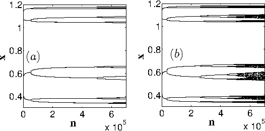
Figure 1: Two examples of cascade of bifurcations type trajectories in the Caputo logistic $\alpha$-family of maps (Eq.(22) with $h=1$ and $G_{K}(x)=x-Kx(1-x)$ ) with $\alpha=0.1$ and $x_{0}=0.001$: (a) for the nonlinearity parameter $K=22.37$ the last bifurcation from the period $T=8$ to the period $T=16$ occurs after approximately $5\times 10^{5}$ iterations; (b) when $K=22.423$ the trajectory becomes chaotic after approximately $5\times 10^{5}$ iterations.

A particular problem related to the differentiation between fractional systems and integer ones, the first bifurcation on CBTT, and related problems of stability of fixed points in discrete fractional systems and transition to chaos in continuous fractional systems are considered in this paper.

Stability of fractional systems was investigated in numerous papers based on various methods (Lyapunov’s direct and indirect methods, Lyapunov function, Routh-Hurwitz criterion, …). Here we’ll list only some of the research papers, reviews, and books on the topic. Paper Matignon is the most cited article on stability of linear fractional differential equations. In application to stability of nonlinear fractional differential equations, we’ll mention papers PRL ; Ahmed ; ElSaka ; StL ; StA ; StLW ; StLB . Some of the results on stability of discrete fractional systems can be found in papers StanislavskyMaps ; StChen ; StJarad ; StMohan ; StDis1 ; StB . The reviews on the topic include papers Rev2009 ; Rev2011 ; Rev2013 and books Petras ; Zhou . Almost all results obtained in the cited papers define sufficient conditions of stability and don’t allow to calculate the ranges of nonlinearity parameters and orders of derivatives for which fixed points are stable.

In this paper we derive the algebraic equations to calculate asymptotically period two sinks of discrete fractional systems, which define the conditions of their appearance, and conjecture that these equations define the values of nonlinearity parameters and orders of derivatives for which fixed points become unstable. This conjecture is numerically verified for the fractional standard and logistic maps. This paper is a continuation of the research on general properties of fractional systems based on the properties of fractional maps Chaos2015 ; ME3 ; ME2 ; Chaos ; ME4 ; ME5 ; DNC ; StanislavskyMaps ; Chaos2014 ; ME6 ; ME9 ; ME10 ; T2009a ; T2009b ; T2 ; T1 ; Fall . In Sec. II we review the most common forms of fractional maps. In Sec. III we derive the equations defining the ranges of nonlinearity parameters and orders of derivatives for which fixed points are stable. Sec. IV presents the summary of our results.

II Fractional/fractional difference maps

In this section some essential definitions and theorems are presented.

II.1 Fractional integrals and derivatives

In this paper we will use the definition of fractional integral introdused by Liouville, which is a generalization of the Cauchy formula for the n-fold integral

$${}_{a}I^{p}_{t}x(t)=\frac{1}{\Gamma(p)}\int^{t}_{a}\frac{x(\tau)d\tau}{(t-\tau)^{1-p}}~{},$$ (1)

where $p$ is a real number, $\Gamma()$ is the gamma function and we’ll assume $a=0$.

The left-sided Riemann-Liouville fractional derivative ${}_{0}D^{\alpha}_{t}x(t)$ is defined for $t>0$ KST ; Podlubny ; SKM as

$${}_{0}D^{\alpha}_{t}x(t)=D^{n}_{t}\ {}_{0}I^{n-\alpha}_{t}x(t)$$

$$=\frac{1}{\Gamma(n-\alpha)}\frac{d^{n}}{dt^{n}}\int^{t}_{0}\frac{x(\tau)d\tau}{(t-\tau)^{\alpha-n+1}}~{},$$ (2)

where $n-1\leq\alpha<n$, $n\in\mathbb{Z}$, $D^{n}_{t}=d^{n}/dt^{n}$.

In the definition of the left-sided Caputo derivative, the order of integration and differentiation in Eq. (2) is switched KST

$${}_{0}^{C}D^{\alpha}_{t}x(t)=_{0}I^{n-\alpha}_{t}\ D^{n}_{t}x(t)$$

$$=\frac{1}{\Gamma(n-\alpha)}\int^{t}_{0}\frac{D^{n}_{\tau}x(\tau)d\tau}{(t-\tau)^{\alpha-n+1}},\quad(n-1<\alpha\leq n).$$ (3)

II.2 Fractional sums and differences

We’ll also use the proposed by Miller and Ross generalization of the forward sum/difference operator MR

$$\Delta x(t)=x(t+1)-x(t)$$ (4)

(see below) and call it simply the fractional sum/difference operator. Nabla fractional difference, which is the generalization of the backward sum/difference operator $\nabla x(t)=x(t)-x(t-1)$ GZ1988 is not considered in this paper.

The fractional sum ($\alpha>0$)/difference ($\alpha<0$) operator deined in MR

$${}_{a}\Delta^{-\alpha}_{t}f(t)=\frac{1}{\Gamma(\alpha)}\sum^{t-\alpha}_{s=a}(t-s-1)^{(\alpha-1)}f(s)$$ (5)

is a fractional generalization of the $n$-fold summation formula ME9 ; GZ1988

$${}_{a}\Delta^{-n}_{t}f(t)=\frac{1}{(n-1)!}\sum^{t-n}_{s=a}(t-s-1)^{(n-1)}f(s)$$

$$=\sum^{t-n}_{s^{0}=a}\sum^{s^{0}}_{s^{1}=a}...\sum^{s^{n-2}}_{s^{n-1}=a}f(s^{n-1}),$$ (6)

where $n\in\mathbb{N}$. In Eq. (5) $f$ is defined on $\mathbb{N}_{a}$ and ${}_{a}\Delta^{-\alpha}_{t}$ on $\mathbb{N}_{a+\alpha}$, where $\mathbb{N}_{t}=\{t,t+1,t+2,...\}$. The falling factorial $t^{(\alpha)}$ is defined as

$$t^{(\alpha)}=\frac{\Gamma(t+1)}{\Gamma(t+1-\alpha)},\ \ t\neq-1,-2,-3,...$$ (7)

and is asymptotically a power function:

$$\lim_{t\rightarrow\infty}\frac{\Gamma(t+1)}{\Gamma(t+1-\alpha)t^{\alpha}}=1,\ \ \ \alpha\in\mathbb{R}.$$ (8)

For $\alpha>0$ and $m-1<\alpha\leq m$ the fractional (left) Riemann-Liouville difference operator is defined (see Atici1 ; Atici2 ) as

$${}_{a}\Delta^{\alpha}_{t}x(t)=\Delta^{m}_{a}\Delta^{-(m-\alpha)}_{t}x(t)$$

$$=\frac{1}{\Gamma(m-\alpha)}\Delta^{m}\sum^{t-(m-\alpha)}_{s=a}(t-s-1)^{(m-\alpha-1)}x(s)$$ (9)

and the fractional (left) Caputo-like difference operator (see Anastas ) as

$${}_{a}^{C}\Delta^{\alpha}_{t}x(t)=_{a}\Delta^{-(m-\alpha)}_{t}\Delta^{m}x(t)$$

$$=\frac{1}{\Gamma(m-\alpha)}\sum^{t-(m-\alpha)}_{s=a}(t-s-1)^{(m-\alpha-1)}\Delta^{m}x(s).$$ (10)

Due to the fact that ${}_{a}\Delta^{\lambda}_{t}$ in the limit $\lambda\rightarrow 0$ approaches the identity operator (see ME9 ; MR ), the definition Eq. (10) can be extended to all real $\alpha\geq 0$ with ${}_{a}^{C}\Delta^{m}_{t}x(t)=\Delta^{m}x(t)$ for $m\in\mathbb{N}_{0}$.

Fractional h-difference operators, which are generalizations of the fractional difference operators, were introduced in hdif1 ; hdif3 . The h-sum operator is defined as

$$(_{a}\Delta^{-\alpha}_{h}f)(t)=\frac{h}{\Gamma(\alpha)}\sum^{\frac{t}{h}-\alpha}_{s=\frac{a}{h}}(t-(s+1)h)^{(\alpha-1)}_{h}f(sh),$$ (11)

where $\alpha\geq 0$, $(_{a}\Delta^{0}_{h}f)(t)=f(t)$, $f$ is defined on $(h\mathbb{N})_{a}$, and ${}_{a}\Delta^{-\alpha}_{h}$ on $(h\mathbb{N})_{a+\alpha h}$. $(h\mathbb{N})_{t}=\{t,t+h,t+2h,...\}$. The $h$-factorial $t^{(\alpha)}_{h}$ is defined as

$$t^{(\alpha)}_{h}=h^{\alpha}\frac{\Gamma(\frac{t}{h}+1)}{\Gamma(\frac{t}{h}+1-\alpha)}=h^{\alpha}\Bigl{(}\frac{t}{h}\Bigr{)}^{(\alpha)},$$ (12)

where $t/h\neq-1,-2,-3,...$. With $m=\lceil\alpha\rceil$ the Riemann-Liouville (left) h-difference is defined as

$$(_{a}\Delta^{\alpha}_{h}x)(t)=(\Delta^{m}_{h}(_{a}\Delta^{-(m-\alpha)}_{h}x))(t)=\frac{h}{\Gamma(m-\alpha)}$$

$$\times\Delta^{m}_{h}\sum^{\frac{t}{h}-(m-\alpha)}_{s=\frac{a}{h}}(t-(s+1)h)^{(m-\alpha-1)}_{h}x(sh)$$ (13)

and the Caputo (left) h-difference is defined as

$$(_{a}\Delta^{\alpha}_{h,*}x)(t)=(_{a}\Delta^{-(m-\alpha)}_{h}(\Delta^{m}_{h}x))(t)=\frac{h}{\Gamma(m-\alpha)}$$

$$\times\sum^{\frac{t}{h}-(m-\alpha)}_{s=\frac{a}{h}}(t-(s+1)h)^{(m-\alpha-1)}_{h}(\Delta^{m}_{h}x)(sh),$$ (14)

where $(\Delta^{m}_{h}x))(t)$ is the $m$th power of the forward $h$-difference operator

$$(\Delta_{h}x)(t)=\frac{x(t+h)-x(t)}{h}.$$ (15)

As it has been noted in hdif1 ; hdif3 , due to the convergence of solutions of fractional Riemann-Liouville h-difference equations when $h\rightarrow 0$ to solutions of the corresponding differential equations, they can be used to solve fractional Riemann-Liouville differential equations numerically.

II.3 Fractional maps

Maps with power-law memory can be introduced directly as a particular form of maps with memory (see papers Chaos2015 ; StanislavskyMaps which contain references and discussions on the topic). The most general form of the convolution-type map with power-law memory introduced in Chaos2015 can be written as

$$x_{n}=\sum^{\lceil\alpha\rceil-1}_{k=1}\frac{c_{k}}{\Gamma(\alpha-k+1)}(nh)^{\alpha-k}$$

$$+\frac{h^{\alpha}}{\Gamma({\alpha})}\sum^{n-1}_{k=0}(n-k)^{\alpha-1}G_{K}(x_{k}),$$ (16)

where $\alpha\geq 0$, $K$ is a parameter, and $h$ is a constant time step between the time instants $t_{n}=a+nh$ and $t_{n+1}$. For a physical interpretation of this formula we consider a system which state is defined by the variable $x(t)$ and evolution by the continuous function $G_{K}(x)$. The value of the state variable at the time $t_{n}$, $x_{n}=x(t_{n})$, is a weighted total of the functions $G_{K}(x_{k})$ from the values of this variable at the past time instants $t_{k}=a+kh$, $0\leq k<n$, $t_{k}=kh$. The weights are the times between the time instants $t_{n}$ and $t_{k}$ to the fractional power $\alpha-1$. Eq.  (16) in the limit $h\rightarrow 0+$ yields the Volterra integral equation of the second kind

$$x(t)=\sum^{\lceil\alpha\rceil-1}_{k=1}\frac{c_{k}}{\Gamma(\alpha-k+1)}(t-a)^{\alpha-k}$$

$$+\frac{1}{\Gamma(\alpha)}\int^{t}_{a}\frac{G_{K}(\tau,x(\tau))d\tau}{(t-\tau)^{1-\alpha}}.\ \ \ (t>a),$$ (17)

This equation is equivalent to the fractional differential equation with the Riemann-Liouville or Gr$\ddot{u}$nvald-Letnikov fractional derivative Chaos2015 ; KBT1 ; KBT2

$${}_{a}^{RL/GL}D^{\alpha}_{t}x(t)=G_{k}(t,x(t)),\ \ 0<\alpha$$ (18)

with the initial conditions

$$(_{a}^{RL/GL}D^{\alpha-k}_{t}x)(a+)=c_{k},\ \ \ k=1,2,...,\lceil\alpha\rceil.$$ (19)

For $\alpha\not\in\mathbb{N}$ we assume $c_{\lceil\alpha\rceil}=0$, which corresponds to a finite value of $x(a)$.

The same map, Eq. (16), called the universal map, represents the solution of the fractional generalization of the differential equation of a periodically (with the period $h$) kicked system (see DNC ; Chaos ; ME5 ; T2009a ; T2009b ; T2 ; T1 for the fractional universal maps and ZasBook in regular dynamics).

To derive the equations of the fractional universal map, which we’ll call the universal $\alpha$-family of maps ($\alpha$-FM) for $\alpha\geq 0$, we start with the differential equation

$$\frac{d^{\alpha}x}{dt^{\alpha}}+G_{K}(x(t-\Delta h))\sum^{\infty}_{k=-\infty}\delta\Bigl{(}\frac{t}{h}-(k+\varepsilon)\Bigr{)}=0,$$ (20)

where $\varepsilon>\Delta>0$, $\alpha\in\mathbb{R}$, $\alpha>0$, and consider it as $\varepsilon\rightarrow 0$. The initial conditions should correspond to the type of the fractional derivative used in Eq. (20). The case $\alpha=2$, $\Delta=0$, and $G_{K}(x)=KG(x)$ corresponds to the equation whose integration yields the regular universal map.

Integration of Eq. (20) with the Riemann-Liouville fractional derivative ${}_{0}D^{\alpha}_{t}x(t)$ and the initial conditions

$$(_{0}D^{\alpha-k}_{t}x)(0+)=c_{k},$$ (21)

where $k=1,...,N$ and $N=\lceil\alpha\rceil$, yields the Riemann-Liouville universal $\alpha$-FM Eq. (16).

Integration of Eq. (20) with the Caputo fractional derivative ${}_{0}^{C}D^{\alpha}_{t}x(t)$ and the initial conditions $(D^{k}_{t}x)(0+)=b_{k}$, $k=0,...,N-1$ yields the Caputo universal $\alpha$-FM

$$x_{n+1}=\sum^{N-1}_{k=0}\frac{b_{k}}{k!}h^{k}(n+1)^{k}$$

$$-\frac{h^{\alpha}}{\Gamma(\alpha)}\sum^{n}_{k=0}G_{K}(x_{k})(n-k+1)^{\alpha-1}.$$ (22)

In this paper we’ll refer to the map Eqs. (16), the RL universal $\alpha$-FM, as the Riemann-Liouville universal map with power-law memory or the Riemann-Liouville universal fractional map; we’ll call the Caputo universal $\alpha$-FM, Eq. (22), the Caputo universal map with power-law memory or the Caputo universal fractional map.

In the case of integer $\alpha$ the universal map converges to $x_{n}=0$ for $\alpha=0$ and $x_{n+1}=x_{n}-hG_{K}(x_{n})$ for $\alpha=1$. and for $\alpha=N=2$ with $p_{n+1}=(x_{n+1}-x_{n})/h$

$$\begin{array}[]{c}\left\{\begin{array}[]{lll}p_{n+1}=p_{n}-hG_{K}(x_{n}),\ \ n\geq 0,\\ x_{n+1}=x_{n}+hp_{n+1},\ \ n\geq 0.\end{array}\right.\end{array}$$ (23)

N-dimensional, with $N\geq 2$, universal maps are investigated in Chaos , where it is shown that they are volume preserving.

II.4 Universal fractional difference map

In what follows we will consider fractional Caputo difference maps - the only fractional difference maps which behavior has been investigated. The following theorem Chaos2014 ; ME9 ; ME10 ; Fall ; DifSum is essential to derive the universal fractional difference map

Theorem 1

For $\alpha\in\mathbb{R}$, $\alpha\geq 0$ the Caputo-like h-difference equation

$$(_{0}\Delta^{\alpha}_{h,*}x)(t)=-G_{K}(x(t+(\alpha-1)h)),$$ (24)

where $t\in(h\mathbb{N})_{m}$, with the initial conditions

$$(_{0}\Delta^{k}_{h}x)(0)=c_{k},\ \ \ k=0,1,...,m-1,\ \ \ m=\lceil\alpha\rceil$$ (25)

is equivalent to the map with $h$-factorial-law memory

$$x_{n+1}=\sum^{m-1}_{k=0}\frac{c_{k}}{k!}((n+1)h)^{(k)}_{h}$$

$$-\frac{h^{\alpha}}{\Gamma(\alpha)}\sum^{n+1-m}_{s=0}(n-s-m+\alpha)^{(\alpha-1)}G_{K}(x_{s+m-1}),$$ (26)

where $x_{k}=x(kh)$, which is called the $h$-difference Caputo universal $\alpha$-family of maps.

In the case of integer $\alpha$ the fractional difference universal map converges to $x_{n+1}=-G_{K}(x_{n})$ for $\alpha=0$, $x_{n+1}=x_{n}-hG_{K}(x_{n})$ for $\alpha=1$, and for $\alpha=N=2$ with $p_{n+1}=(x_{n+1}-x_{n})/h$

$$\begin{array}[]{c}\left\{\begin{array}[]{lll}p_{n+1}=p_{n}-hG_{K}(x_{n}),\ \ n\geq 1,\ \ p_{1}=p_{0},\\ x_{n+1}=x_{n}+hp_{n+1},\ \ n\geq 0.\end{array}\right.\end{array}$$ (27)

N-dimensional, with $N\geq 2$, difference universal maps are volume preserving Chaos2014 .

All above considered universal maps in the case $\alpha=2$ yield the standard map if $G_{K}(x)=K\sin(x)$ (harmonic nonlinearity) and we’ll call them the standard $\alpha$-families of maps. When $G_{K}(x)=x-Kx(1-x)$ (quadratic nonlinearity) in the one-dimensional case all maps yield the regular logistic map and we’ll call them the logistic $\alpha$-families of maps.

III Period two sinks and stability of fixed points

In fractional systems not only the speed of convergence of trajectories to the periodic sinks but also the way in which convergence occurs depends on the initial conditions. As $n\rightarrow\infty$, all trajectories in Fig. 2 converge to the same period two ($T=2$) sink (as in Fig. 2 c), but for small values of the initial conditions $x_{0}$ all trajectories first converge to the $T=1$ trajectory which then bifurcates and turns into the $T=2$ sink converging to its limiting value. As $x_{0}$ increases, the bifurcation point $n_{bif}$ gradually evolves from the right to the left (Fig. 2(a)). Ignoring this feature may result (as in Fall and some other papers) in very messy bifurcation diagrams.

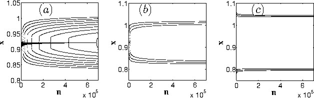
Figure 2: Asymptotically period two trajectories for the Caputo logistic $\alpha$-family of maps with $\alpha=0.1$ and $K=15.5$: (a) nine trajectories with the initial conditions $x_{0}=0.29+0.04i$, $i=0,1,...,8$ ($i=0$ corresponds to the rightmost bifurcation); (b) $x_{0}=0.61+0.06i$, $i=1,2,3$; (c) $x_{0}=0.95+0.04i$, $i=1,2,3$. As $n\rightarrow\infty$ all trajectories converge to the limiting values $x_{lim1}=0.80629$ and $x_{lim2}=1.036030$ (see Eq (71)). The unstable fixed point is $x_{lim0}=(K-1)/K=0.93548$.

In this paper we consider the asymptotic stability of periodic points. A periodic point is asymptotically stable if there exists an open set such that all trajectories with initial conditions from this set converge to this point as $t\rightarrow\infty$. It is known from the study of the ordinary nonlinear dynamical systems that as a nonlinearity parameter increases the system bifurcates. This means that at the point (value of the parameter) of birth of the $T=2^{n+1}$ sink, the $T=2^{n}$ sink becomes unstable. In this section we will investigate the $T=2$ sinks of discrete fractional systems and apply our results to analyze stability of the systems’ fixed points.

III.1 $0<\alpha<1$

When $0<\alpha<1$, all introduced in this paper forms of the universal $\alpha$-family of maps, Eqs. (16),  (22), (26), can be written in the form

$$x_{n+1}=x_{0}-\sum^{n}_{k=0}\tilde{G}(x_{k})U(n-k+1).$$ (28)

In this formula $\tilde{G}(x)=h^{\alpha}G_{K}(x)/\Gamma(\alpha)$ and $x_{0}$ is the initial condition ($x_{0}=0$ in Eq. (16)). In fractional maps, Eqs. (16) and (22),

$$U_{\alpha}(n)=n^{\alpha-1},\ \ \ \ U_{\alpha}(1)=1$$ (29)

and in fractional difference maps, Eq. (26),

$$U_{\alpha}(n)=(n+\alpha-2)^{(\alpha-1)},\ \ \ \$$

$$U_{\alpha}(1)=(\alpha-1)^{(\alpha-1)}=\Gamma(\alpha).$$ (30)

For $n=2N$ Eq. (28) can be written (after subtracting $x_{2N}$) as

$$x_{2N+1}=x_{2N}-\tilde{G}(x_{2N})U_{\alpha}(1)$$

$$+\sum^{N}_{n=1}\tilde{G}(x_{2N-2n+1})\Bigl{(}U_{\alpha}(2n-1)-U_{\alpha}(2n)\Bigr{)}$$

$$+\sum^{N}_{n=1}\tilde{G}(x_{2N-2n})\Bigl{(}U_{\alpha}(2n)-U_{\alpha}(2n+1)\Bigr{)}.$$ (31)

The terms $U_{\alpha}(2n-1)-U_{\alpha}(2n)$ are of the order $n^{\alpha-2}$. If we assume that in the limit $n\rightarrow\infty$ period $T=2$ sink exists,

$$x_{o}=\lim_{n\rightarrow\infty}x_{2n+1},\ \ \ \ x_{e}=\lim_{n\rightarrow\infty}x_{2n},$$ (32)

then the series in Eq.(31) converge absolutely. In the limit $n\rightarrow\infty$ Eq.(31) converges to

$$x_{o}-x_{e}=\Bigl{[}\tilde{G}(x_{o})-\tilde{G}(x_{e})\Bigr{]}W_{\alpha},$$ (33)

where $W_{\alpha}$ is a converging series

$$W_{\alpha}=\sum^{\infty}_{n=1}\Bigl{[}U_{\alpha}(2n-1)-U_{\alpha}(2n)\Bigr{]},$$ (34)

which can be computed numerically with $U_{\alpha}(n)$ defined either by Eq. (29) or by Eq. (30).

Now, instead of subtracting, let’s add $x_{2N}$ to $x_{2N+1}$:

$$x_{2N+1}+x_{2N}=2x_{0}-\sum^{2N}_{n=1}\Bigl{[}\tilde{G}(x_{2N-n+1})+$$

$$\tilde{G}(x_{2N-n})\Bigr{]}U_{\alpha}(n)-\tilde{G}(x_{0})U_{\alpha}(2N+1).$$ (35)

If $T=2$ sink exists, then, in the limit $n\rightarrow\infty$, the left-hand side (LHS) of Eq. (35), as well as the first term on the right-hand side (RHS) and the last term of this equation, is finite. Expressions in the brackets in Eq. (35) tend to the limit $\tilde{G}(x_{o})+\tilde{G}(x_{e})$. Because the series $\sum^{\infty}_{n=1}U_{\alpha}(n)$ is diverging, the only case in which Eq. (35) can be true is when

$$\tilde{G}(x_{o})+\tilde{G}(x_{e})=0.$$ (36)

Equations which define the existence and value of the asymptotic $T=2$ sink can be written as

$$\begin{array}[]{c}\left\{\begin{array}[]{lll}G_{K}(x_{o})+G_{K}(x_{e})=0,\\ x_{o}-x_{e}=\frac{W_{\alpha}}{\Gamma(\alpha)}h^{\alpha}\Bigl{[}G_{K}(x_{o})-G_{K}(x_{e})\Bigr{]}.\end{array}\right.\end{array}$$ (37)

• It is easy to see that the fixed point, defined by the equation $G_{K}(x_{o})=0$ is a solution of the system Eq. (37).

• As it was mentioned above, when $h\rightarrow 0$, fractional difference equations converge to the corresponding fractional differential equations. As $h\rightarrow 0$, the second equation from the system Eq. (37) leads to $x_{o}-x_{e}\rightarrow 0$. This implies that in fractional differential equations of the order $0<\alpha<1$ transition from a fixed point to periodic trajectories will never happen. A strict proof of the impossibility of periodic trajectories (except fixed points) in autonomous fractional systems described by the fractional differential equation

  $$\frac{d^{\alpha}x}{dt^{\alpha}}=G_{K}(x(t)),\ \ \ 0<\alpha<1$$ (38)

  with the Caputo or Riemann-Liouville fractional derivative was given in PerC1 (Theorem 9 there). Nonexistence of periodic trajectories and the fact that in regular dynamics transition to chaos occurs through cascades of the period doubling bifurcations, leads us to the following conjecture

  Conjecture 2

  Chaos does not exist in continuous fractional systems of the orders $0<\alpha<1$.

III.2 $1<\alpha<2$

For $1<\alpha<2$ map equations Eqs. (16), (22), (26), can be written in the form

$$x_{n+1}=x_{0}+f(\alpha)[h(n+1)]^{\beta}p_{0}$$

$$-h\sum^{n}_{k=0}\tilde{G}(x_{k})U_{\alpha}(n-k+1)+hf_{1}(n).$$ (39)

Here $\tilde{G}(x)=h^{\alpha-1}G_{K}(x)/\Gamma(\alpha)$, $x_{0}$ and $U(n)$ are defined the same way as in Eqs. (28), (29), and (30), $p_{0}$ is the initial momentum ($b_{k}$ or $c_{k}$ in corresponding formulae), $\beta$ is equael to $1$ in Eqs. (22), (26) and $\alpha-1$ in Eq. (16) $f(\alpha)$ is $1$ in Eqs. (22), (26) and $1/\Gamma(\alpha)$ in Eq. (16), and $f_{1}(n)=0$ in Eqs. (16), (22) and $f_{1}(n)=h^{\alpha-1}G(x_{0})(n-1+\alpha)^{(\alpha-1)}/\Gamma(\alpha)\sim n^{\alpha-1}$ in Eq. (26).

If we define

$$p_{n+1}=\frac{x_{n+1}-x_{n}}{h},$$ (40)

then, taking into account that $U_{\alpha}(0)=0$, from Eq. (39) follows

$$p_{n+1}=\tilde{f}(n)p_{0}$$

$$-\sum^{n}_{k=0}\tilde{G}(x_{k})\tilde{U}_{\alpha}(n-k+1)+f_{1}(n)-f_{1}(n-1),$$ (41)

where

$$\tilde{U}_{\alpha}(n)=U_{\alpha}(n)-U_{\alpha}(n-1)$$

$$=\begin{array}[]{c}\left\{\begin{array}[]{lll}n^{\alpha-1}-(n-1)^{\alpha-1}\sim n^{\alpha-2}\\ {\rm and}\ \ \tilde{U}_{\alpha}(1)=1\ \ {\rm in\ \ Eqs.~{}(\ref{EqDir}),~{}(\ref{FrCMapx})};\\ (n+\alpha-2)^{(\alpha-1)}-(n+\alpha-3)^{(\alpha-1)}\\ =(\alpha-1)(n+\alpha-3)^{(\alpha-2)}\\ =(\alpha-1)U_{\alpha-1}(n)\sim n^{\alpha-2}\\ {\rm and}\ \ \tilde{U}_{\alpha}(1)=\Gamma(\alpha)\ \ {\rm in\ \ Eq.~{}(\ref{FalFacMap_h})},\end{array}\right.\end{array}$$ (49)

$f_{1}(n)-f_{1}(n-1)=0$ in Eqs. (16), (22) and $f_{1}(n)-f_{1}(n-1)\sim n^{\alpha-1}$ in Eq. (26), $\tilde{f}(n)=1$ in Eqs. (22), (26) and $\tilde{f}(n)\sim n^{\alpha-2}$ in Eq. (16). Note, that the definition of $\tilde{U}_{\alpha}(1)$ in Eq. (49) and $U_{\alpha}(1)$ in Eqs. (29), (30) are identical.

Assuming existence of the $T=2$ sink and limits $x_{o}$ and $x_{e}$ are defined by Eq. (32), the limiting values for $p$ are defined by

$$p_{o}=\lim_{n\rightarrow\infty}p_{2n+1}=\lim_{n\rightarrow\infty}\frac{x_{2n+1}-x_{2n}}{h}=\frac{x_{o}-x_{e}}{h}$$

$${\rm and}\ \ p_{e}=\lim_{n\rightarrow\infty}p_{2n}=-p_{o}.$$ (50)

As in the derivation of Eqs. (33) and (36), if we add and subtract expressions for $p_{2N+1}$ and $p_{2N}$, we’ll arrive at relations

$$p_{o}-p_{e}=\Bigl{[}\tilde{G}(x_{o})-\tilde{G}(x_{e})\Bigr{]}\tilde{W}_{\alpha}$$ (51)

and

$$\tilde{G}(x_{o})+\tilde{G}(x_{e})=0,$$ (52)

where $\tilde{W}_{\alpha}$ is a converging series

$$\tilde{W}_{\alpha}=\sum^{\infty}_{n=1}\Bigl{[}\tilde{U}_{\alpha}(2n-1)-\tilde{U}_{\alpha}(2n)\Bigr{]}.$$ (53)

Let’s note that with $U_{\alpha}(n)=n^{\alpha-1}$, as defined in Eq. (29), $\tilde{W}$ is identical to the introduced in ME2 $V_{\alpha l}$ defined as

$$\tilde{W}_{\alpha}=V_{\alpha l}=\sum^{\infty}_{n=1}(-1)^{n+1}\Bigl{[}n^{\alpha-1}-(n-1)^{\alpha-1}\Bigr{]}.$$ (54)

High accuracy algorithm for calculating $V_{\alpha l}$ is presented in Appendix to ME4 . For $U(n)$ defined by Eq. (30) $\tilde{W}$ was calculated in Chaos2014 . Taking into account that converging series Eq. (53) can be written as

$$\tilde{W}_{\alpha}=\tilde{U}_{\alpha 1}-\sum^{\infty}_{n=1}\Bigl{[}\tilde{U}_{\alpha}(2n)-\tilde{U}_{\alpha}(2n+1)\Bigr{]},$$ (55)

where

$$\tilde{U}_{\alpha 1}=\begin{array}[]{c}\left\{\begin{array}[]{lll}1\ \ {\rm in\ \ Eqs.~{}(\ref{EqDir}),~{}(\ref{FrCMapx})},\\ \Gamma(\alpha)\ \ {\rm in\ \ Eq.~{}(\ref{FalFacMap_h})},\end{array}\right.\end{array}$$ (59)

and using absolute convergence of series Eq. (34) (and, correspondingly, the series on the first line of Eq. (III.2) below), for $0<\alpha<1$ we can write

$$\tilde{W}_{\alpha}=\tilde{U}_{\alpha 1}-\sum^{\infty}_{n=1}\Bigl{\{}\Bigl{[}{U}_{\alpha}(2n)-{U}_{\alpha}(2n-1)\Bigr{]}-$$

$$-\Bigl{[}{U}_{\alpha}(2n+1)-{U}_{\alpha}(2n)\Bigr{]}\Bigr{\}}$$

$$=\tilde{U}_{\alpha 1}+\sum^{\infty}_{n=1}\Bigl{[}{U}_{\alpha}(2n-1)-{U}_{\alpha}(2n)\Bigr{]}$$ (60)

$$-\sum^{\infty}_{n=1}\Bigl{[}{U}_{\alpha}(2n)-{U}_{\alpha}(2n+1)\Bigr{]}=W_{\alpha}+\tilde{U}_{\alpha 1}$$

$$-U_{\alpha}(2)+U_{\alpha}(3)-U_{\alpha}(4)+U_{\alpha}(5)-...=2W_{\alpha}.$$

Let us notice that in fractional difference maps Eq. (55) can be written as

$$\tilde{W}_{\alpha}=(\alpha-1)\Gamma(\alpha-1)-(\alpha-1)\sum^{\infty}_{n=1}\Bigl{[}U_{\alpha-1}(2n)-$$

$$U_{\alpha-1}(2n+1)\Bigr{]}=(\alpha-1)W_{\alpha-1}=\frac{\alpha-1}{2}\tilde{W}_{\alpha-1}.$$ (61)

Finally, the equations which define the existence and value of the asymptotic $T=2$ sink for $0<\alpha<2$ can be written as

$$\begin{array}[]{c}\left\{\begin{array}[]{lll}G_{K}(x_{o})+G_{K}(x_{e})=0,\\ x_{o}-x_{e}=\frac{\tilde{W}_{\alpha}}{2\Gamma(\alpha)}h^{\alpha}\Bigl{[}G_{K}(x_{o})-G_{K}(x_{e})\Bigr{]},\end{array}\right.\end{array}$$ (62)

where $\tilde{W}_{\alpha}$ is defined by Eqs. (55), (59). Notice that according to Eq (55) $\tilde{W}_{1}=1$.

• As in the case $0<\alpha<1$, for $1<\alpha<2$ the fixed point, defined by the equation $G_{K}(x_{o})=0$ is a solution of the system Eq. (62).

• As $h\rightarrow 0$, fractional difference equations converge to the corresponding fractional differential equations and $x_{o}-x_{e}\rightarrow 0$, which implies that in fractional differential equations of the order $1<\alpha<2$ transition from a fixed point to periodic trajectories will never happen. Now we may formulate a stronger conjecture:

  Conjecture 3

  Chaos does not exist in continuous fractional systems of the orders $0<\alpha<2$.

III.3 Examples

Now we’ll consider application of the results from this section to the introduced at the end of Section II fractional and fractional difference standard ($G_{K}(x)=K\sin(x)$) and logistic ($G_{K}(x)=x-Kx(1-x)$ ) $\alpha$-families of maps.

III.3.1 Standard $\alpha$-families of maps

With $G_{K}(x)=K\sin(x)$ all above considered forms of the universal map for $\alpha=2$ converge to the regular standard map and they are called the standard $\alpha$-families of maps. These families of maps are usually considered on a torus (mod $2\pi$). The first equation of the system Eq. (62) yields

$$\sin\frac{x_{o}+x_{e}}{2}\cos\frac{x_{o}-x_{e}}{2}=0,$$ (63)

which on $x\in[-\pi,\pi]$ yields two solutions

$${\rm symmetric\ \ point}\ \ x_{osy}=-x_{esy}\ \ {\rm and}\$$

$${\rm shift}-\pi\ \ {\rm point}\ \ x_{osh}=x_{esh}-\pi.$$ (64)

Then, the second equation of Eq. (62) yields the equation which together with Eq. (64) defines two $T=2$ sinks for $0<\alpha<2$

$$\sin x_{osy}=\frac{2\Gamma(\alpha)}{\tilde{W}_{\alpha}h^{\alpha}K}x_{osy}$$ (65)

and

$$\sin x_{osh}=\frac{\pi\Gamma(\alpha)}{\tilde{W}_{\alpha}h^{\alpha}K}.$$ (66)

The symmetric $T=2$ sink appears when

$$h^{\alpha}|K|>h^{\alpha}|K_{C1s}|=\frac{2\Gamma(\alpha)}{\tilde{W}_{\alpha}}$$ (67)

and the shift-$\pi$ $T=2$ sink appears when

$$h^{\alpha}|K|>\frac{\pi}{2}h^{\alpha}|K_{C1s}|.$$ (68)

Figure 3: 2D bifurcation diagrams for fractional (solid thing lines) and fractional difference (bold and dashed lines) Caputo standard (a) and $h=1$ logistic (b) maps. Fist bifurcation, transition from the stable fixed point to the stable period two ($T=2$) sink, occurs on the bottom curves. $T=2$ sink (in the case of standard $\alpha$-families of maps antisymmetric T=2 sink with $x_{n+1}=-x_{n}$) is stable between the bottom and the middle curves. Transition to chaos occurs on the top curves. For the standard fractional map transition from $T=2$ to $T=4$ sink occurs on the line below the top line (the third from the bottom line). Period doubling bifurcations leading to chaos occur in the narrow band between the two top curves. All bottom curves, as well as the next to the bottom in (a), are obtained using formulae Eqs. (67), (68), and (72). Two dashed lines for $1<\alpha<2$ in (b) are obtained by interpolation. The remaining lines are results of the direct numerical simulations. Stability of the fixed point for the fractional difference logistic $\alpha$-family of maps is calculated using both, Eq. (72) (bold solid line) and the direct numerical simulations (a dashed line branching from the solid line). The difference is due to the slow, as $n^{-\alpha}$ (see Chaos2014 ), convergence of trajectories to the $T=2$ sink for small $\alpha$ ($x$ vs. $K$, fixed $\alpha$, bifurcation diagrams used to find the first bifurcation were calculated on trajectories after 5000 iterations).

III.3.2 Logistic $\alpha$-families of maps

With $G_{K}(x)=x-Kx(1-x)$ all above considered forms of the universal map for $\alpha=1$ converge to the regular logistic map and they are called the logistic $\alpha$-families of maps. Th system Eq. (62) becomes

$$\begin{array}[]{c}\left\{\begin{array}[]{lll}(1-K)(x_{o}+x_{e})+K(x_{o}^{2}+x_{e}^{2})=0,\\ x_{o}-x_{e}=\frac{\tilde{W}_{\alpha}}{2\Gamma(\alpha)}h^{\alpha}(x_{o}-x_{e})[1-K+(x_{o}+x_{e})]\end{array}\right.\end{array}$$ (69)

Two fixed point solutions with $x_{o}=x_{e}$ are $x_{o}=0$, stable for $K<1$, and $x_{o}=(K-1)/K$.

The $T=2$ sink is defined by the equation

$$x_{o}^{2}-\Bigl{(}\frac{2\Gamma(\alpha)}{\tilde{W}Kh^{\alpha}}+\frac{K-1}{K}\Bigr{)}x_{o}+\frac{2\Gamma^{2}(\alpha)}{(\tilde{W}Kh^{\alpha})^{2}}+\frac{(K-1)\Gamma(\alpha)}{\tilde{W}K^{2}h^{\alpha}}=0,$$ (70)

which has solutions

$$x_{o}=\frac{K_{C1s}+K-1\pm\sqrt{(K-1)^{2}-K_{C1s}^{2}}}{2K}$$ (71)

defined when

$$K\geq 1+\frac{2\Gamma(\alpha)}{\tilde{W}h^{\alpha}}=1+K_{C1s}\ \ {\rm or}\ \ K\leq 1-\frac{2\Gamma(\alpha)}{\tilde{W}h^{\alpha}}=1-K_{C1s}$$ (72)

The first inequality of Eq. (72) was derived in ME4 for $h=1$ and $1<\alpha<2$. In this paper we consider $K>0$ and $h\leq 1$. It follows from the definition, Eq. (55), that $\tilde{W}<\tilde{U}_{1}$, which is either 1 or $\Gamma(\alpha)$, and it is known that $\Gamma(\alpha)>0.885$ for $\alpha>0$. Then, $2\Gamma(\alpha)/(\tilde{W}h^{\alpha})>1$ and we may ignore the second of the inaquolities in Eq. (72). We may also note that the fixed point $x=(K-1)/K$ is stable when

$$1\leq K<K_{C1l}=1+\frac{2\Gamma(\alpha)}{\tilde{W}h^{\alpha}}=1+K_{C1s}.$$ (73)

IV Conclusion

Figs. 3 a and b, the two-dimensional bifurcation diagrams, present results of the computer simulations of the fractional and fractional difference standard and logistic maps. Low curves on these diagrams are obtained using Eqs. (67), (68), and (72). They are in good agreement with the results (also used to calculate all other curves) obtained by the direct numerical simulations by calculating $x$ vs. $K$ bifurcation diagrams for various $\alpha\in(0,2)$ after 5000 iterations. Slight difference in Fig. 3 b for the fractional difference logistic map for $\alpha<0.2$ is probably due to the slow, as $\sim n^{-\alpha}$ convergence of trajectories to the fixed points. This confirms the validity of Eq. (62) to calculate the coordinates of the asymptotic $T=2$ sinks and the points of the first bifurcations for the discrete fractional/fractional difference maps. The continuous limits of the considered in this paper discrete maps are fractional differential equations and from the consideration presented in this paper we may conclude that chaos is impossible in systems described by equations

$$\frac{d^{\alpha}x}{dt^{\alpha}}=f(x)$$ (74)

with $0<\alpha<2$.

There are still many unanswered questions related to the behavior of fractional systems. They include:

• What is the nature and the corresponding analytic description of the bifurcations on a single trajectory of a fractional system?

• What kind of self-similarity can be found in CBTT?

• How to describe a self-similar behavior corresponding to the bifurcation diagrams of fractional systems? Can constants, similar to the Feigenbaum constants be found?

• Can cascade of bifurcations type trajectories be found in continuous systems?

This paper is a small step in investigation of the fractional dynamical systems and we hope that the following works will lead to more complete description of fractional (with power-law memory) systems which have many applications in biological, social, and physical systems.

References

- (1) J. A. Tenreiro Machado, F. B. Duarte, G. M. Duarte, Int. J. Bifurcation Chaos 22, 1250249 (2012).
- (2) J. A. Tenreiro Machado, C. M. A. Pinto, A. M. Lopes, Signal Process 107, 246 (2015).
- (3) V. E. Tarasov and V. V. Tarasova, Int. J. Management Social Sciences 5, 327 (2016).
- (4) M. J. Kahana, Foundations of human memory (Oxford University Press, New York, 2012).
- (5) D. C. Rubin and A. E. Wenzel, Psychological Review 103, 743 (1996).
- (6) J. T. Wixted, Journal of Experimental Psychology: Learning, Memory, and Cognition 16, 927 (1990).
- (7) J. T. Wixted and E. Ebbesen, Psychological Science 2, 409 (1991).
- (8) J. T. Wixted and E. Ebbesen, Memory & Cognition 25, 731 (1997).
- (9) C. Donkin and R. M. Nosofsky, Psychol. Sci. 23, 625 (2012).
- (10) J. R. Anderson, Learning and memory: An integrated approach (Wiley, New York 1995).
- (11) A. L. Fairhall, G. D. Lewen, W. Bialek, and R. R. de Ruyter van Steveninck, Nature 412, 787 (2001).
- (12) D, A. Leopold, Y. Murayama, and N. K. Logothetis, Cerebral Cortex 413, 422 (2003).
- (13) A. Toib, V. Lyakhov, and S. Marom, Journal of Neuroscience 18, 1893 (1998).
- (14) N. Ulanovsky, L. Las, D. Farkas, and I. Nelken, Journal of Neuroscience 24, 10440 (2004).
- (15) M. S. Zilany, I. C. Bruce, P. C. Nelson, and L. H. Carney, J. Acoust. Soc. Am. 126, 2390 (2009).
- (16) B. N. Lundstrom, A. L. Fairhall, and M. Maravall, J. Neuroscience 30, 5071 (2010).
- (17) B. N. Lundstrom, M. H. Higgs, W. J. Spain, and A. L. Fairhall, Nature Neuroscience 11, 1335 (2008).
- (18) C. Pozzorini, R. Naud, S. Mensi, and W. Gerstner, Nat. Neurosci. 16, 942 (2013).
- (19) M. Edelman, Chaos 25, 073103 (2015).
- (20) M. Edelman, 2011, Commun. Nonlin. Sci. Numer. Simul. 16, 4573 (2011).
- (21) A. S. Deshpande, V. Daftardar-Gejji Chaos, Solitons and Fractals 102, 119 (2017).
- (22) M. Edelman and V. E. Tarasov, Phys. Lett. A 374, 279 (2009).
- (23) M. Edelman, Chaos 23, 033127 (2013).
- (24) M. Edelman, and L. A. Taieb, in: Advances in Harmonic Analysis and Operator Theory; Series: Operator Theory: Advances and Applications, Eds: A. Almeida, L. Castro, and F.-O. Speck 229, 139–155 (Springer, Basel, 2013).
- (25) J. Jagan Mohan, Communications in Applied Analysis 20, 585 (2016).
- (26) J. Jagan Mohan, Fractional Differential Calculus 7, 339 (2017).
- (27) I. Area, J. Losada, and J. J. Nieto, Abstract and Applied Analysis 2014, 392598 (2014).
- (28) E. Kaslik and S. Sivasundaram, Nonlinear Analysis. Real World Applications 13, 1489 (2012).
- (29) M. S. Tavazoei and M. Haeri, Automatica 45, 1886 (2009).
- (30) J. Wang, M. Feckan, and Y. Zhou, Commun in Nonlin. Sci. Numer. Simul. 18, 246 (2013).
- (31) M. Yazdani and H. Salarieh, Automatica 47, 1837 (2011).
- (32) G. M. Zaslavsky, A. A. Stanislavsky, and M. Edelman, Chaos 16, 013102 (2006).
- (33) M. Edelman, in: Nonlinear Dynamics and Complexity; Series: Nonlinear Systems and Complexity, Eds.: A. Afraimovich, A. C. J. Luo, and X. Fu, 79–120 (New York, Springer, 2014).
- (34) M. Edelman, Discontinuity, Nonlinearity, and Complexity 1, 305 (2013).
- (35) A. A. Stanislavsky, Eur. Phys. J. B 49, 93 (2006).
- (36) J. Cermak and L. Nechvatal, Nonlin. Dyn. 87, 939 (2017).
- (37) D. Matignon, Proceedings of the International Meeting on Automated Compliance Systems and the International Conference on Systems, Man, and Cybernetics (IMACS-SMC 96), pp. 963–968 (Lille, France, 1996).
- (38) I. Grigorenko and E. Grigorenko, Phys. Rev. Lett. 91,034101 (2003).
- (39) E. Ahmed, A. M. A. El-Sayed, and Hala A.A. El-Saka, Phys. Lett. A 358, 1 (2006).
- (40) H. A. El-Saka, E. Ahmed, M. I. Shehata, and A. M. A. El-Sayed, Nonlinear Dyn. 56, 121 (2009).
- (41) Y. Li, Y. Q. Chen, and I. Podlubny, Comput. Math. Appl. 59, 1810 (2010).
- (42) N. Aguila-Camacho, M. A. Duarte-Mermoud, and J. A. Gallegos, Commun. Nonlin. Sci. Numer. Simul. 19, 2951 (2014).
- (43) T. Li and Y. Wang, Discrete Dynamics in Nature and Society 2014, 724270, (2014).
- (44) B. K. Lenka and S. Banerjee Nonlinear Dyn. 85, 167 (2016).
- (45) A. A. Stanislavsky, Chaos 16, 043105 (2006).
- (46) F. Chen and Z. Liu, J. Appl. Math. 2012, 879657, (2012).
- (47) F. Farad, T. Abdeljawad, D. Baleanu, and K. Bicen, Abstr. Appl. Anal. 2012, 476581 (2012).
- (48) J. Jagan Mohan, N. Shobanadevi, and G. V. S. R. Deekshitulu, Italian J. Pure Appl. Math. 32, 165 (2014).
- (49) Wyrwas, M., Pawluszewicz, E., and Girejko, E.: Kybernetika 15, 112–136 (2015).
- (50) D. Baleanu, G.-C. Wu, Y.-R. Bai, and F.-L. Chen, Commun. Nonlin. Sci. Numer. Simul. 48, 520 (2017).
- (51) I. Petras, Frac. Calc. Appl. Anal. 12, 269 (2009).
- (52) C. P. Li and F. R. Zhang, Eur. Phys. J. Special Topics 193, 27 (2011).
- (53) M. Rivero, S. V. Rogozin, J. A. T. Machado, and J. J. Trujilo, Math. Probl. Eng. 2013, 356215 (2013).
- (54) I. Petras, Fractional-Order Nonlinear Systems (Springer, Berlin, 2011).
- (55) Y. Zhou, Basic Theory of Fractional Differential Equations (World Scientific, Singapore, 2014).
- (56) M. Edelman, Chaos 24, 023137 (2014).
- (57) M. Edelman, in: International Conference on Fractional Differentiation and Its Applications (ICFDA), 2014, DOI: 10.1109/ICFDA.2014.6967376, 1–6 (2014).
- (58) M. Edelman, Discontinuity, Nonlinearity, and Complexity 4, 391 (2015).
- (59) M. Edelman, in: Chaotic, Fractional, and Complex Dynamics: New Insights and Perspectives; Series: Understanding Complex Systems, Eds.: M. Edelman, E. Macau, and M. A. F. Sanjuan, 147–171 (eBook, Springer, 2018).
- (60) V. E. Tarasov, J. Phys. A 42, 465102 (2009).
- (61) V. E. Tarasov, J. Math. Phys. 50, 122703 (2009).
- (62) V. E. Tarasov, Fractional Dynamics: Application of Fractional Calculus to Dynamics of Particles, Fields and Media (HEP, Springer, Beijing, Berlin, Heidelberg, 2011).
- (63) V. E. Tarasov and G.M. Zaslavsky, J. Phys. A 41, 435101 (2008).
- (64) G.-C. Wu, D. Baleanu, S.-D. Zeng, Phys. Lett. A 378, 484 (2014).
- (65) S. G Samko, A. A. Kilbas, and O. I. Marichev, Fractional Integrals and Derivatives Theory and Applications (Gordon and Breach, New York, 1993).
- (66) A. A. Kilbas, H. M. Srivastava, and J. J. Trujillo, Theory and Application of Fractional Differential Equations (Elsevier, Amsterdam, 2006)
- (67) I. Podlubny, Fractional Differential Equations (Academic Press, San Diego, 1999).
- (68) K. S. Miller, and B. Ross, In: H. M. Srivastava, and S. Owa, (eds.) Univalent Functions, Fractional Calculus, and Their Applications. 139–151 (Ellis Howard, Chichester, 1989).
- (69) H. L. Gray and N. F. Zhang, Mathematics of Computation 50, 513 (1988).
- (70) F. Atici and P. Eloe, Proc. Am. Math. Soc. 137, 981 (2009).
- (71) F. Atici and P. Eloe, Electron. J. Qual. Theory Differ. Equ. Spec. Ed. I3, 1 (2009).
- (72) G. A. Anastassiou, http://arxiv.org/abs/0911.3370 (2009).
- (73) N. R. O. Bastos, R. A. C. Ferreira, and D. F. M. Torres, Discrete-time fractional variational problems. Signal Processing 91, 513 (2011).
- (74) R. A. C. Ferreira and D. F. M. Torres, Appl. Anal. Discrete Math. 5, 110 (2011).
- (75) A. A. Kilbas, B. Bonilla, and J. J. Trujillo, Dokl. Math. 62, 222 (2000).
- (76) A. A. Kilbas, B. Bonilla, and J. J. Trujillo, Demonstratio Math. 33, 583 (2000).
- (77) G. M. Zaslavsky, Hamiltonian Chaos and Fractional Dynamics (Oxford University Press, Oxford, 2008).
- (78) F. Chen, X. Luo, and Y. Zhou, Adv.Differ.Eq. 2011, 713201 (2011).