The Boundary of the Future

Abstract

We prove that the boundary of the future of a surface $K$ consists precisely of the points $p$ that lie on a null geodesic orthogonal to $K$ such that between $K$ and $p$ there are no points conjugate to $K$ nor intersections with another such geodesic. Our theorem has applications to holographic screens and their associated light sheets and in particular enters the proof that holographic screens satisfy an area law.

I Theorem

In this paper, we prove the following theorem establishing necessary and sufficient conditions for a point to be on the boundary of the future of a surface in spacetime. (An analogous theorem holds for the past of $K$.)

Theorem 1.

Let $(M,g)$ be a smooth, globally hyperbolic spacetime and let $K$ be a smooth codimension-two submanifold of $M$ that is compact and acausal. Then a point $b\in M$ is on the boundary of the future of $K$ if and only if all of the following statements hold:

1. $b$ lies on a future-directed null geodesic $\gamma$ that intersects $K$ orthogonally.

2. $\gamma$ has no points conjugate to $K$ strictly before $b$.

3. $\gamma$ does not intersect any other null geodesic orthogonal to $K$ strictly between $K$ and $b$.

Theorem 1 enumerates the conditions under which a light ray, launched normally from a surface, can exit the boundary of the future of that surface and enter its chronological future. In essence, this happens only when the light ray either hits another null geodesic launched orthogonally from the surface or when the light ray encounters a caustic, in a sense that will be made precise in terms of special conditions on the deviation vectors for a family of infinitesimally-separated geodesics. These two possibilities for the fate of the light ray are illustrated in Fig. 1.

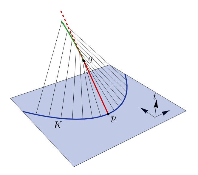
Figure 1: Possibilities for how a null geodesic orthogonal to a surface can exit the boundary of its future. In this example, a parabolic surface $K$ (blue line) lies in a particular spatial slice. A future-directed null geodesic (red line) is launched orthogonally from $p$. At $q$, it encounters a caustic, entering the interior of the future of $K$ (red dashed line). The point $q$ is conjugate to $K$. Other null geodesics orthogonal to $K$ (black lines) encounter nonlocal intersections with other such geodesics along the green line, where they exit the boundary of the future of $K$.

The theorem is useful for characterizing the causal structure induced by spatial surfaces. In particular, if $K$ splits a Cauchy surface into two parts, then Theorem 1 implies that the four orthogonal null congruences fully characterize the associated split of the spacetime into four portions: the future and past of $K$ and the domains of dependence of each of the two spatial sides (see Fig. 2). This is of particular interest when $K$ is a holographic screen CEB2 . Then some of the orthogonal congruences form light sheets CEB1 such that the entropy of matter on a light sheet is bounded by the area of $K$. This relation makes precise the notion that the universe is like a “hologram” Tho93 ; Sus95 ; FisSus98 and should be described as such in a quantum gravity theory. Such holographic theories have indeed been identified for a special class of spacetimes Mal97 .

Specifically, Theorem 1 plays a role in the recent proof of a novel area theorem for holographic screens BouEng15a ; BouEng15b , where it was assumed without proof. It also enters the analogous derivation of a related Generalized Second Law in cosmology BouEng15c from the Quantum Focusing Conjecture BouFis15a .

Although our motivation lies in applications to General Relativity and quantum gravity, we stress that the theorem itself is purely a statement about Lorentzian geometry. It does not assume Einstein’s equations and so in particular does not assume any conditions on the stress tensor of matter.

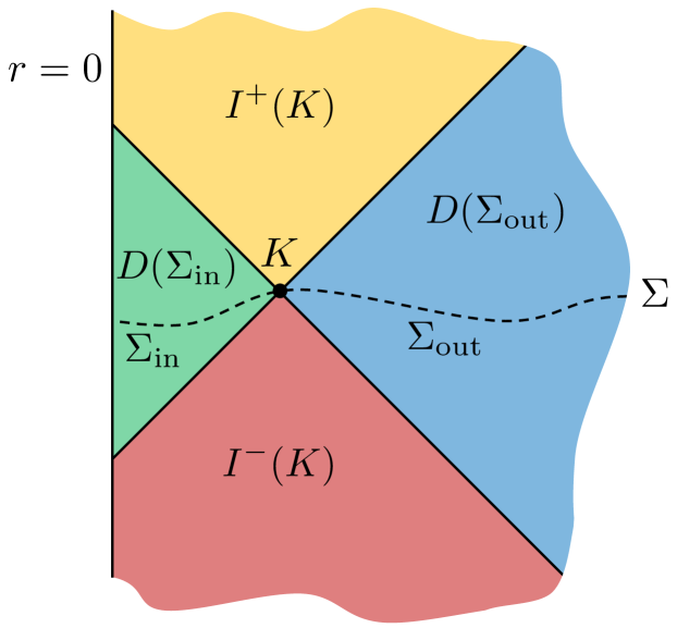
Figure 2: In this generic Penrose diagram, the codimension-two surface $K$ (black dot) splits a Cauchy surface $\Sigma$ (dashed line) into two parts $\Sigma_{\rm in}$, $\Sigma_{\rm out}$. This induces a splitting of the spacetime $M$ into four parts: the past and future of $K$ (red, yellow) and the domains of dependence of $\Sigma_{\rm in}$ and $\Sigma_{\rm out}$ (green, blue) BouEng15b . Theorem 1 guarantees that this splitting is fully characterized by the four orthogonal null congruences originating on $K$ (black diagonal lines).

Related Work.

Parts of the “only if” direction of the theorem are a standard textbook result Wald , except for $(iii)$, which we easily establish. The “if” direction is nontrivial and takes up the bulk of our proof.

LABEL:Beem considers the cut locus, i.e., the set of all cut points associated with geodesics starting at some point $p\in M$. Given a geodesic $\gamma$ originating at $p$, a future null cut point, in particular, can be defined in terms of the Lorentzian distance function or equivalently as the final point on $\gamma$ that is in the boundary of the future of $p$. As shown in Theorem 5.3 of LABEL:Beem, if $q$ is the future null cut point on $\gamma$ of $p$, then either $q$ corresponds to the first future conjugate point of $p$ along $\gamma$, or another null geodesic from $p$ intersects $\gamma$ at $q$, or both. Our theorem can be viewed as an analogous result for geodesics orthogonal to codimension-two surfaces and a generalization of our theorem implies the result of LABEL:Beem as a special case. The codimension-two surfaces treated by our theorem are of significant physical interest due to the important role of holographic screens in the study of quantum gravity (see, e.g., Ref. NettaAron2017 for very recent results on the coarse-grained black hole entropy). We encountered nontrivial differences in proving the theorem for surfaces. Moreover our condition ($ii$) places stronger constraints on the associated deviation vector, as we discuss in Sec. II.2.

The previously known parts of the “only if” direction of Theorem 1 were originally established in the context of proving singularity theorems Penrose2 ; Hawking2 . It would be interesting to see whether Theorem 1 can be used to derive new or stronger results on the formation or the cosmic censorship of spacetime singularities.

Generalizations.

As we are only concerned with the causal structure, the metric can be freely conformally rescaled. Thus, a version of Theorem 1 still holds for noncompact $K$, as long as it is compact in the conformal completion of the spacetime, i.e., in a Penrose diagram. A situation in which this may be of interest is for surfaces anchored to the boundary of anti-de Sitter space.

Furthermore, the theorem can be generalized to surfaces of codimension other than two, but in that case we can say less about the type of conjugate point that orthogonal null geodesics may encounter. We will discuss this further in Sec. III.

Notation.

Throughout, we use standard notation for causal structure. A causal curve is one for which the tangent vector is always timelike or null. The causal (respectively, chronological) future of a set $S$ in our spacetime $M$, denoted by $J^{+}(S)$ (respectively, $I^{+}(S)$) is the set of all $q\in M$ such that there exists $p\in S$ for which there is a future-directed causal (respectively, timelike) curve in $M$ from $p$ to $q$. For the past ($I^{-}(S)$, $J^{-}(S)$, etc.), similar definitions apply. We will denote the boundary of a set $S$ by $\dot{S}$. Standard results Wald include that $I^{\pm}(S)$ is open and that $\dot{J}^{\pm}(S)=\dot{I}^{\pm}(S)$. We will call a set $S$ acausal if there do not exist distinct $p,q\in S$ for which there is a causal path in $M$ from $p$ to $q$. A spacetime is said to be globally hyperbolic if it contains no closed causal curves and if $J^{+}(p)\cap J^{-}(q)$ is compact for all $p,q\in M$. Equivalently Geroch , $M$ has the topology of $\Sigma\times\mathbb{R}$ for some Cauchy surface $\Sigma$; that is, $\Sigma$ is a surface for which, for all $p\in M$, every inextendible timelike curve through $p$ intersects $\Sigma$ exactly once.

Outline.

In Sec. II, we review the notion of a conjugate point and establish some useful lemmas. In Sec. III, we prove Theorem 1.

II Conjugate Points to a Surface

II.1 Exponential Map

Let $(M,g)$ be a smooth, globally hyperbolic spacetime of dimension $n>2$. Thus, $M$ is a manifold with metric $g$ of signature $(-,+,\ldots,+)$. (As already noted, we will be concerned only with the causal structure of $M$, so $g$ need only be known up to conformal transformations.)

For $p\in M$, let $T_{p}M$ be the tangent vector space at $p$ and let $TM\equiv\bigcup_{p\in M}\{p\}\times T_{p}M$ be the tangent bundle of $M$. $TM$ has a natural topology that makes it a manifold of dimension $2n$. In the open subsets associated with charts of $M$, $TM$ is diffeomorphic to open subsets of $\mathbb{R}^{2n},$ corresponding to $n$ coordinates for the location of $p\in M$ and $n$ components of a tangent vector $v\in T_{p}M$. The tangent space of $TM$ at $(p,v)$ is

$$T_{p,v}TM=T_{p}M\times T_{v}T_{p}M.$$ (1)

For every $(p,v)\in TM$, there is a unique inextendible geodesic,

$$c_{p,v}:(a,b)\to M,~{}s\mapsto c_{p,v}(s),$$ (2)

where $a,b\in\mathbb{R}\cup\{-\infty,\infty\}$, with affine parameter $s$ and tangent vector $v\in T_{p}M$ given by the pushforward of $d/ds$ by $c_{p,v}$ at the point $p=c_{p,v}(0)\in M$. It is convenient to include the degenerate curves obtained with $v=0$.

Definition 2.

The exponential map is defined by:

$$\exp\,:~{}TM\to M,~{}(p,v)\mapsto c_{p,v}(1).$$ (3)

Restrictions of $\exp$ to submanifolds of $TM$ are frequently of interest. To study the congruence of geodesics emanating from a given point, one may restrict to $\exp_{p}:\,T_{p}M\to M\,,~{}v\mapsto c_{p,v}(1)$. Moreover, one can define the differential of $\exp_{p}$, $\exp_{p*}:T_{v}T_{p}M\rightarrow T_{c_{p,v}(1)}M$, which describes how $\exp_{p}v$ varies due to small changes in $v$. See Fig. 3 for an illustration of the exponential map and its differential. In this paper, we will consider a different restriction suited to the study of the geodesics orthogonal to a given spatial surface; we will define the differential in more detail for this restriction below.

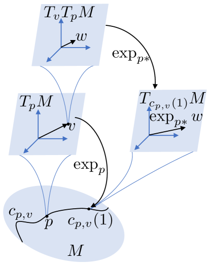
Figure 3: An illustration of the exponential map $\exp$, which takes a vector in $TM$ to a point in $M$, and the Jacobian of the exponential map, which takes a vector in the tangent space $TTM$ of $TM$ to a vector in $TM$.

Let $K\subset M$ be a smooth submanifold. We consider the normal bundle

$$NK\equiv\bigcup_{p\in K}\{p\}\times T_{p}K^{\perp},$$

where $T_{p}K^{\perp}$ is the two-dimensional tangent vector space perpendicular to $K$ at $p$. The normal bundle has the structure of an $n$-dimensional manifold. Its tangent space at $(p,v)\in NK$ is

$$T_{p,v}NK=T_{p}K\times T_{v}T_{p}K^{\perp}.$$ (4)

Here, $T_{p}K$ is the tangent space of $p$ in the manifold $K$; that is, $T_{p}K$ is the subspace of $T_{p}M$ normal to $T_{p}K^{\perp}$. Note that $T_{p}K$ is of the same dimension as $K$.

Definition 3.

The surface-orthogonal exponential map

$$\exp_{K}\,:~{}NK\to M\,,~{}(p,v)\mapsto c_{p,v}(1)$$ (5)

is the restriction of $\exp$ to $NK$.

Definition 4.

The Jacobian or differential of the exponential map is given by

$$\exp_{K*}\,:~{}T_{p,v}NK\to TM\,,~{}w\mapsto\exp_{K*}w.$$ (6)

It is a linear map between vectors that captures the response of $\exp_{K}$ to small variations in its argument. It is defined by requiring that $(\exp_{K*}w)(f)=w(f\mathbin{\mathchoice{\vbox{\hbox{$\scriptstyle\!\circ\!$}}}{\vbox{\hbox{$\scriptstyle\!\circ\!$}}}{\vbox{\hbox{$\scriptscriptstyle\!\circ\!$}}}{\vbox{\hbox{$\scriptscriptstyle\!\circ\!$}}}}\exp_{K})$ for any function $f:\,M\to\mathbb{R}$. Note $\exp_{K*}w$ is the pushforward of $w$ by $\exp_{K}$. If $x^{\alpha}$ are coordinates in an open neighborhood of $(p,v)\in NK$ and $y^{\beta}$ are coordinates in an open neighborhood of $\exp_{K}(p,v)\in M$ and we write the vectors in coordinate form, $w=\sum w^{\alpha}(\partial/\partial x^{\alpha})$ and $\exp_{K*}w=\sum\hat{w}^{\beta}(\partial/\partial y^{\beta})$, then the components are related by the Jacobian matrix,

$$\hat{w}^{\beta}=\sum_{\alpha}\frac{\partial y^{\beta}}{\partial x^{\alpha}}w^{\alpha}.$$ (7)

See Fig. 4 for an illustration of $\exp_{K}$, $\exp_{K*}$, and the various tangent spaces used in this paper.

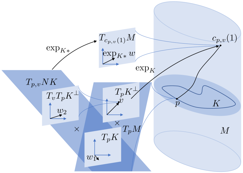
Figure 4: An illustration of the surface-orthogonal exponential map $\exp_{K}$ evaluated at $p\in K$, which takes a vector in $T_{p}K^{\perp}$ to a point $c_{p,v}(1)$ in $M$. Here, as in text, the tangent space at $p$, $T_{p}M$, is broken up as a product $T_{p}K^{\perp}\times T_{p}K$. Also shown is the Jacobian $\exp_{K*}$ at $v\in T_{p}K^{\perp}$, which takes a vector $w=(w_{1},w_{2})\in T_{p,v}NK=T_{p}K\times T_{v}T_{p}K^{\perp}$ to a vector in $T_{c_{p,v}(1)}M$.

Definition 5.

A Jacobian is an isomorphism if it is invertible, i.e., if it has no eigenvectors with eigenvalue zero.

Since $(M,g)$ and $K$ are smooth, $\exp_{K}$ is smooth. The inverse function theorem rudin thus implies the following.

Lemma 6.

If the Jacobian $\exp_{K*}$ at $(p,v)\in NK$ is an isomorphism, then $\exp_{K}$ is a diffeomorphism of an open neighborhood of $(p,v)$ onto an open neighborhood of $\exp_{K}(p,v)\in M$.

Definition 7.

The exponential map $\exp_{K}$ is called singular at $(p,v)\in NK$ if $\exp_{K*}$ is not an isomorphism. Then $(p,v)$ is called a conjugate point in $NK$.

II.2 Jacobi Fields

It is instructive to relate the above definition of conjugate point to an equivalent definition in terms of Jacobi fields.

Definition 8.

Let $Q$ be an open set in $\mathbb{R}^{2}$ and let $f:\,Q\to M,\,(r,s)\mapsto f(r,s)$ be a smooth map. If the curves of constant $r$ and varying $s$, $\gamma_{r}:Q\to M,s\mapsto f(r,s)$, are geodesics in $M$, then $f$ is called a one-parameter family (or congruence) of geodesics.

Definition 9.

Let $\partial_{s}$ denote the partial derivative with respect to $s$. It follows from the above definition that the pushforward $S\equiv f_{*}(\partial_{s})\in TM$ is tangent to any geodesic $\gamma_{r}$. Similarly, $R\equiv f_{*}(\partial_{r})\in TM$ is tangent to any curve $\mu_{s}:Q\to M,r\mapsto f(r,s)$ at fixed $s$. For general families of curves, $R$ represents the deviation vector field of the congruence. In the special case of a geodesic congruence, $R$ restricted to any $\gamma_{r}$ is called a Jacobi field on $\gamma_{r}$.

Remark 10.

The Jacobi field $R$ satisfies the geodesic deviation equation on $Q$,

$$D^{2}_{S}R=\mathcal{R}(S,R)S,$$ (8)

where $\mathcal{R}(A,B)\equiv[D_{A},D_{B}]-D_{[A,B]}$ is the curvature tensor Hicks ; Wald and $D_{V}=V^{\mu}\nabla_{\mu}$ is the covariant derivative, defined with respect to the Levi-Civita connection, along a vector $V$.

The exponential map can be used to generate a one-parameter family of geodesics and its derivative $\exp_{*}$ generates the associated Jacobi fields. We first recall the more familiar case of geodesics through a point $p$, generated by $\exp_{p}$, as follows.

Remark 11.

Let $\hat{R},\hat{S}\in T_{p}M$ and let $\tilde{R}$ and $\tilde{S}$ be the naturally associated constant vector fields in $TT_{p}M$. Then $f(r,s)=\exp_{p}[s(\hat{S}+r\hat{R})]$ is smooth and defines a one-parameter family of geodesics. Its tangent vector field is $S=\left.\exp_{p*}\right|_{s(\hat{S}+r\hat{R})}(\tilde{S}+r\tilde{R})$ and its deviation or Jacobi field is $R=\left.\exp_{p*}\right|_{s(\hat{S}+r\hat{R})}s\tilde{R}$. It is clear from this construction that $\exp_{p}$ is singular (i.e., $\exp_{p*}$ fails to be an isomorphism) at $s(\hat{S}+r\hat{R})$ if and only if there exists a nontrivial Jacobi field of the geodesic $\gamma_{r}$ that vanishes at $f(r,s)$ and $f(r,0).$ This establishes the equivalence of two common definitions of conjugacy to a point $p$.

Remark 12.

A conjugate point in a geodesic congruence with tangent vector $k^{\mu}$ corresponds to a caustic, which is a point at which the expansion $\theta=\nabla_{\mu}k^{\mu}$ goes to $-\infty$.

We turn to the case relevant to this paper: a one-parameter family of geodesics orthogonal to a smooth, compact, acausal, codimension-two submanifold $K$. (For example, $K$ could be a topological sphere at an instant of time.) Subject to this restriction, the map $f$ and vector fields $R$ and $S$ are defined as before, with $T_{p}M$ replaced by $T_{p}K^{\perp}$. One can choose the parameters $(r,s)$ such that $f(r,0)\in K$ and $f(0,0)=p$. The map $\nu:r\mapsto(f(r,0),S|_{(r,0)})$ is a smooth curve in $NK$ with tangent vector $\bar{R}\in TNK$. From this curve, the one-parameter family can be recovered as

$$f(r,s)=\exp_{f(r,0)}sS|_{(r,0)}=\exp_{K}(f(r,0),sS|_{(r,0)}).$$ (9)

Remark 13.

We will be interested in the Jacobi field $R\equiv f_{*}\partial_{r}$ only along one geodesic, say $\gamma$ at $r=0$. By Eq. (8) this depends only on the initial data $S$ and $\bar{R}$ at $p$. Thus $R|_{(0,s)}$ will be the same for any curve $\nu$ with tangent vector $\bar{R}$ at $(p,S|_{(0,0)})\in NK$. Conversely, one can extend any given $\bar{R}$ at $(p,S|_{(0,0)})\in NK$ to a (non-unique) one-parameter family of geodesics by picking such a curve $\nu$. We now take advantage of this freedom in order to find an explicit expression for the Jacobi field in terms of $\exp_{K*}$.

By Eq. (4), one can uniquely decompose $\bar{R}=(\check{R},\tilde{R})$, with $\check{R}\in T_{p}K$ and $\tilde{R}\in T_{S}T_{p}K^{\perp}$. Let $\pi$ be the defining projection of the fiber bundle, $\pi:NK\to K$. Then $\mu\equiv\pi(\nu)$ is a curve on $K$ with tangent vector $\check{R}$ at $p$. Let $f(r,0)=\mu(r)$.

Further, let $S|_{(r,0)}\in T_{f(r,0)}K^{\perp}$ be defined by $K$-normal parallel transport of the vector $S|_{(0,0)}+r\hat{R}\in T_{p}K^{\perp}$ along $\mu$ from $p$ to $\mu(r)$. Here $\hat{R}\in T_{p}K^{\perp}$ is the vector naturally associated with $\tilde{R}\in T_{S}T_{p}K^{\perp}.$ Similarly, we define $\tilde{S}\in T_{S}T_{p}K^{\perp}$ to be the vector naturally associated with $\left.S\right|_{(0,0)}.$

Lemma 14.

With the above choices and definitions, Eq. (9) yields a suitable one-parameter family of geodesics. The corresponding Jacobi field and tangent vector along $\gamma$ can be written as:

$$R|_{(0,s)}\equiv\left.f_{*}\partial_{r}\right|_{(0,s)}=\left.\exp_{K*}\right|_{(p,sS|_{(0,0)})}(\check{R},s\tilde{R})$$ (10)

and

$$S|_{(0,s)}\equiv\left.f_{*}\partial_{s}\right|_{(0,s)}=\left.\exp_{K*}\right|_{(p,sS|_{(0,0)})}(0,\tilde{S}),$$ (11)

respectively.

See App. A for a proof of Lemma 14 via a direct calculation.

We note that $\check{R}$ and $\tilde{R}$ encode the initial value and derivative, respectively, of $R$, in accordance with the initial value problem set up in Remark 13. From Eq. (10), we obtain a criterion for conjugacy equivalent to that of Def. 7:

Remark 15.

In the above notation, the map $\exp_{K}$ is singular at $(p,sS|_{(0,0)})\in NK$ if and only if the geodesic $\gamma$ possesses a nontrivial Jacobi field that vanishes at $\exp_{K}(p,sS|_{(0,0)})$ and is tangent to $K$ at $p.$

Specifically, our interest lies in null geodesics orthogonal to $K$. We now show that their conjugate points satisfy an additional criterion on the associated eigenvector of $\exp_{K*}$.

Lemma 16.

Let $\gamma$ be a geodesic orthogonal to $K$ at $p$, with conjugate point $(p,sS|_{(0,0)})\in NK$. By Def. 7 there exists a nonzero vector $\bar{R}\in T_{p,sS|_{(0,0)}}NK$ such that $\left.\exp_{K*}\right|_{(p,sS|_{(0,0)})}\bar{R}=0$. If $\gamma$ is null, i.e., if $\|{S|_{(0,0)}}\|=0$, then the projection of $\bar{R}$ onto $T_{p}K$ is nonvanishing: $\check{R}\neq 0$.

Proof.

By Eqs. (10) and (11), the Jacobi field $R|_{(0,s)}$ is orthogonal to $\gamma$ at two points: at $p$ (by construction) and (trivially) at the assumed conjugate point. By Lemma 8.7 of Ref. oneill , this implies that $R_{(0,s)}\perp S|_{(0,s)}$ for all $s$. Again using Eqs. (10) and  (11), along with linearity of $\exp_{K*}$, this implies that $\tilde{R}\perp\tilde{S}$ and thus $\exp_{K*}|_{(p,sS|_{(0,0)})}(0,s\tilde{R})\perp S.$

Prior to the conjugate point, the map $\exp_{K*}$ is a linear isomorphism; hence it maps the (1+1)-dimensional subspace $T_{S}T_{p}K^{\perp}\ni\tilde{R}$ of $T_{p,S}NK$ into a (1+1)-dimensional subspace $\exp_{K*}T_{S}T_{p}K^{\perp}$ of $T_{f(0,1)}M$. This subspace contains both the null tangent vector $S|_{(0,s)}$ and the component $\exp_{K*}|_{(p,sS|_{(0,0)})}(0,s\tilde{R})$ of the Jacobi field $R$, which is itself a Jacobi field since our choice of initial data $\bar{R}$ was arbitrary. In a (1+1)-dimensional space, the only vectors orthogonal to a null vector $S$ are proportional to $S$. The general solution to Eq. (8) for a Jacobi field proportional to the tangent vector $S$ is $(\alpha+\beta s)S|_{(0,s)}$. Therefore $\exp_{K*}|_{(p,sS|_{(0,0)})}(0,s\tilde{R})$ must have this form for some real constants $\alpha,\beta$. At $s=0$, $\exp_{K*}|_{(p,sS|_{(0,0)})}(0,s\tilde{R})$ vanishes trivially, so $\alpha=0$.

Now, suppose $\check{R}=0$, so $R|_{(0,s)}$ is just $\beta sS|_{(0,s)}$. Since our Jacobi field is nontrivial and $S$ does not vanish, we must have $\beta\neq 0$. Thus, $R|_{(s,0)}$ vanishes only at $p$ and hence cannot vanish at $\exp_{K}(p,sS|_{(0,0)})$. This contradiction implies that $\check{R}\neq 0$. ∎

We now define a refinement of the notion of a conjugate point.

Definition 17.

Let $\gamma(s)$ be a geodesic orthogonal to $K$ at $p$, with $\gamma(0)=p$ and with conjugate point $(p,v)$. Then there exists a nontrivial Jacobi field $R(s)\in TM$ that vanishes at $q=\exp_{K}(p,v)$ and is tangent to $K$ at $p.$ We say that $q$ is conjugate to (the surface) $K$ if $R$ is nonvanishing at $p.$

Remark 18.

By Lemma 16, $\check{R}\neq 0$, so the Jacobi field associated with $\bar{R}$ as defined in Eq. (10) does not vanish at $p$ and hence, if $(p,sS|_{(0,0)})\in NK$ is a conjugate point, then the point $\exp_{K}(p,sS|_{(0,0)})$ is conjugate to $K$ for $\gamma$ null.

Moreover, we can similarly define the notion of a point conjugate to another point.

Definition 19.

Given a nontrivial Jacobi field $R$ for a segment $\gamma$ of a geodesic such that $R$ vanishes at $p$ and $q$, we say that $q$ is conjugate to (the point) $p$.

See Fig. 5 for an illustration of the two types of conjugate points defined in Defs. 17 and 19.

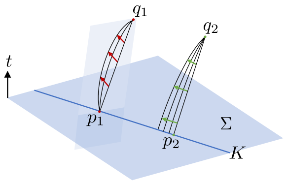
Figure 5: The two types of conjugate points defined in Defs. 17 and 19. The point $q_{1}$ is conjugate to the point $p_{1}$, with the Jacobi field illustrated by the red arrows. The point $q_{2}$ is conjugate to the surface $K$ (blue line), at the point $p_{2}$, with the Jacobi field illustrated by the green arrows. Geodesics orthogonal to $K$ are shown in black. If a general conjugate point lies along an orthogonal null geodesic, then by Lemma 16 there exists a Jacobi field such that the conjugate point is of the surface type. Hence, this type of conjugacy appears in Theorem 1.

III Proof of the Theorem

We now prove Theorem 1.

Proof.

For the “only if” direction, we may assume that $b\in\dot{I}^{+}(K)$. Then conclusions $(i),(ii)$ are already established explicitly elsewhere in the literature (e.g., Theorem 9.3.11 of LABEL:Wald and Theorem 7.27 of LABEL:Penrose; see also Lemma VII of LABEL:Penrose2, as well as LABEL:Hawking2).

Conclusion $(iii)$ follows by contradiction: let $\gamma^{\prime}$ be a distinct null geodesic orthogonal to $K$ that intersects $\gamma$ at some point $q$ strictly between $b$ and $K$. By acausality of $K$, $\gamma^{\prime}\cap K$ is a single point, $p^{\prime}$, which is distinct from $q$. Hence, $K$ can be connected to $b$ by a causal curve that is not an unbroken null geodesic, namely, by following $\gamma^{\prime}$ from $p^{\prime}$ to $q$ and $\gamma$ from $q$ to $b$. By Proposition 4.5.10 in Ref. HawEll , this implies that some $r\in K$ can be joined to $b$ by a timelike curve, in contradiction with $b\in\dot{I}^{+}(K)$. Hence, no such $\gamma^{\prime}$ can exist.

The “if” direction of the theorem states that if $(i),(ii),(iii)$ hold, then $b\in\dot{I}^{+}(K)$. We will prove the following equivalent statement: If $b\notin\dot{I}^{+}(K)$ satisfies $(i)$, then $b$ will fail to satisfy $(ii)$ or $(iii)$.

Let the geodesic $\gamma(s)$ guaranteed by $(i)$ be parametrized so that $\gamma(0)=p\equiv\gamma\cap K$ and $\gamma(1)=b$. By $(i)$, $b\in J^{+}(K)$, the causal future of $K$. By assumption, $b\notin\dot{I}^{+}(K)=\dot{J}^{+}(K)$, so it follows that $b\in I^{+}(K)$, the chronological future of $K$. Since $p\in\dot{I}^{+}(K)$, there exists an $s_{*}$ between 0 and 1 where $\gamma$ leaves the boundary of the future:

$$s_{*}\equiv\sup\gamma^{-1}(\gamma([0,1])\cap\dot{I}^{+}(K)).$$ (12)

The point where $\gamma$ leaves $\dot{I}^{+}{(K)}$, $q\equiv\gamma(s_{*})$, lies in $\dot{I}^{+}(K)$. Thus $s_{*}<1$. Moreover, $s_{*}>0$ by the obvious generalization of Proposition 4.5.1 in LABEL:HawEll and achronality of $K$. We conclude that

$$p\in\dot{I}^{-}(q)\cap K,~{}~{}q\neq b,~{}\text{and}~{}q\neq p.$$ (13)

Recall that $q=\gamma(s_{*})$ is the future-most point on $\gamma$ that is not in $I^{+}(K)$. Let $s_{n}$ be a strictly decreasing sequence of real numbers that converges to $s_{*}$. That is, $s_{n}>s_{*}$ and, for $n$ sufficiently large, the points $q_{n}\equiv\gamma(s_{n})$ exist and lie in $I^{+}(K)$. Now, since $K$ is acausal and $M$ is globally hyperbolic, there exists a Cauchy surface $\Sigma\supset K.$ Given $p_{1},p_{2}\in M$, define $C(p_{1},p_{2})$ to be the set of all causal curves from $p_{1}$ to $p_{2}$. Since by Corollary 6.6 of LABEL:Penrose $C(\Sigma,q_{n})$ is compact, it is closed and bounded. Thus, $C(K,q_{n})\subset C(\Sigma,q_{n})$ is bounded. Consider a sequence of curves $\mu_{m}$ from $K$ to $q_{n}$. By Lemma 6.2.1 of LABEL:HawEll, the limit curve $\mu$ of $\{\mu_{m}\}$ is causal; since $K$ is compact and thus contains its limit points, $\mu$ runs from $K$ to $q_{n}$, so $\mu\in C(K,q_{n})$. Hence, $C(K,q_{n})$ is closed and therefore compact. Since the proper time is an upper semicontinuous function on $C(\Sigma,q_{n})$, it attains its maximum over a compact domain, so we conclude in analogy with Theorem 9.4.5 of LABEL:Wald that there exists a timelike geodesic $\gamma_{n}$ that maximizes the proper time from $K$ to $q_{n}$. By Theorem 9.4.3 of LABEL:Wald, $\gamma_{n}$ is orthogonal to $K$.

By construction, the point $q$ is a convergence point (and hence a limit point) of the sequence $\{\gamma_{n}\}$. By the time-reverse of Lemma 6.2.1 of Ref. HawEll , there exists, through $q$, a causal limit curve $\gamma^{\prime}$ of the sequence $\{\gamma_{n}\}$. This curve must intersect $K$ because all $\gamma_{n}$ intersect $K$ and $K$ is compact. Since $\gamma^{\prime}$ passes through $q\in\dot{I}^{+}(K)$, it must not be smoothly deformable to a timelike curve since $I^{+}(K)$ is open. Thus, by Theorem 9.3.10 of LABEL:Wald, $\gamma^{\prime}$ must be a null geodesic orthogonal to $K$, so if $\gamma^{\prime}\neq\gamma$, condition $(iii)$ fails to hold. See Fig. 6 for an illustration.

The only alternative is that $\gamma$ is the only limit curve of the sequence $\{\gamma_{n}\}$. In this case, $\{\gamma_{n}\}$ contains a subsequence whose convergence curve is $\gamma$. From now on, let $\{\gamma_{n}\}$ denote this subsequence. Orthogonality to $K$ of the $\gamma_{n}$ implies that we can write

$$q_{n}=\exp_{K}(p_{n},v_{n}),$$ (14)

where $p_{n}=\gamma_{n}\cap K$, for some vector $v_{n}\in T_{p_{n}}K^{\perp}$ tangent to $\gamma_{n}$. But since $q_{n}\in\gamma$, we can also write

$$q_{n}=\exp_{K}(p,k_{n}),$$ (15)

where $k_{n}$ is tangent to $\gamma$. Thus, every $q_{n}$ has a non-unique pre-image.

By the above construction, the sequences $\{(p,k_{n})\}$ and $\{(p_{n},v_{n})\}$ in $NK$ each have $(p,v)$ as their limit point, where $q=\exp_{K}(p,v)$. Hence there exists no open neighborhood $\cal O$ of $(p,v)$ such that $\exp_{K}$ is a diffeomorphism of $\cal O$ onto an open neighborhood of $q$. By Lemma 6, it follows that $\exp_{K}$ is singular at $(p,v)$, i.e., $(p,v)$ is a conjugate point. By Lemma 16 and Remark 18, $q$ is conjugate to $K$. Thus, condition $(ii)$ fails to hold; again, see Fig. 6. ∎

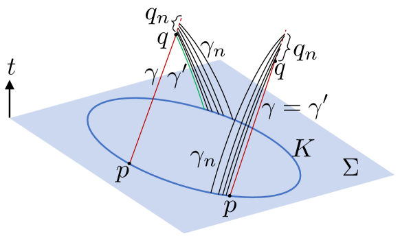
Figure 6: Possibilities in the proof. The sequence of timelike geodesics $\gamma_{n}$ (black) connects $K$ with a sequence of points $q_{n}\in I^{+}(K)$ on the orthogonal null geodesic $\gamma$ (red) that joins $p\in K$ with $q$, after which $\gamma$ leaves $\dot{I}^{+}(K)$ (red dashed). In the case on the left, $\gamma^{\prime}$ (green) is distinct from $\gamma$, so condition (iii) fails. In the case on the right, $\gamma^{\prime}=\gamma$, which we prove corresponds to a failure of condition (ii).

Remark 20.

The fact that $K$ had codimension two was only important in the last step in the proof of Theorem 1, i.e., going from knowing that $(p,v)$ is a conjugate point to showing that $q$ is conjugate to the surface $K$. For $K$ a compact, acausal submanifold that is not of codimension two, the steps in the proof of Theorem 1 still establish that $(p,v)$ is a conjugate point in the sense of Def. 7. Moreover, that the corresponding Jacobi field is orthogonal to $S$ remains true without the codimension-two assumption (see the proof of Lemma 16) and the one-parameter family of geodesics is orthogonal to $K$ (because it was defined via normal parallel transport). As a result, the Jacobi field defines a deviation of $\gamma$ in terms of only orthogonal null geodesics (as proven in, e.g., Corollary 10.40 of LABEL:oneill), but in general that will not mean that $q$ is conjugate to the surface $K$ in the sense of Def. 17. Specifically, the Jacobi field is not necessarily nonvanishing at $K$ if $K$ has codimension greater than two.

Acknowledgments It is a pleasure to thank Jason Koeller for initial collaboration on this project. We also thank Netta Engelhardt, Zachary Fisher, Stefan Leichenauer, and Robert Wald for helpful discussions and correspondence. We thank Umberto Lupo for pointing out Refs. X ; Y to us after this paper first appeared. This work was supported in part by the Berkeley Center for Theoretical Physics, by the National Science Foundation (award numbers PHY-1521446, PHY-1316783), by FQXi, and by the U.S. Department of Energy under contract DE-AC02-05CH11231. G.N.R. is supported by the Miller Institute for Basic Research in Science at the University of California, Berkeley.

Appendix A Proof of Lemma 14

We now prove Lemma 14 by direct calculation.

Proof.

We wish to show that

$$R|_{(0,s)}\equiv\left.f_{*}\partial_{r}\right|_{(0,s)}=\left.\exp_{K*}\right|_{(p,sS|_{(0,0)})}(\check{R},s\tilde{R})$$ (16)

and

$$S|_{(0,s)}\equiv\left.f_{*}\partial_{s}\right|_{(0,s)}=\left.\exp_{K*}\right|_{(p,sS|_{(0,0)})}(0,\tilde{S}),$$ (17)

where

$$f(r,s) =\exp_{f(r,0)}sS|_{(r,0)}$$ (18)

$$=\exp_{K}(f(r,0),sS|_{(r,0)}),$$

as defined in Sec. II.2.

Using the definition of the pushforward, we can write $f_{*}\partial_{r}|_{(0,s)}$ as the differential $\exp_{K*}$, associated with $f$ in Eq. (18), evaluated along the tangent direction $sS|_{(0,0)}$,

$$R|_{(0,s)}\equiv \left.f_{*}\partial_{r}\right|_{(0,s)}$$ (19)

$$= \left.\exp_{K*}\right|_{(p,sS|_{(0,0)})}(\check{R},s\phi_{*}(\partial_{r}S|_{(r,0)})|_{r=0}).$$

In the second line, we used the definition of $\check{R}$ as the tangent to $\mu(r)$ at $p$, along with linearity of $\exp_{K*}$. We have again used the notation $\phi_{*}$ for the identity map between vectors in $T_{p}M$ and their naturally associated counterparts in $T_{S}T_{p}M$.

Next, we must evaluate the derivative of $S$, $\phi_{*}(\partial_{r}S|_{(r,0)})|_{r=0}\in T_{S}T_{p}K^{\perp}$. Let us write $S|_{(r,0)}$ as an explicit function of both the parameter $r$ along the path $\mu(r)\equiv f(r,0)\in K$ and the vector $S|_{(0,0)}+r\hat{R}\in T_{p}K^{\perp}$ that is normal parallel transported along $\mu$ from $\mu(0)=p$ to $\mu(r)$:

$$S|_{(r,0)} =S(r,S|_{(0,0)}+r\hat{R})|_{r_{1}=r_{2}=r}$$ (20)

$$\equiv S(r_{1},r_{2})|_{r_{1}=r_{2}=r},$$

so that the derivative in question can be written as $\phi_{*}\partial_{r}S(r,S|_{(0,0)}+r\hat{R})|_{r=0}$. Since $S(r_{1},r_{2})$ is defined by normal parallel transporting a particular vector ($S|_{(0,0)}+r\hat{R}$) in $T_{p}K^{\perp}$ to $\mu(r_{1})$, its variation with respect to $r_{1}$ gives the normal part of the covariant derivative of $S$ along $\mu$, which vanishes, i.e., $\partial_{r_{1}}S(r_{1},r_{2})=0$. Hence,

$$\frac{\partial}{\partial r}\left[S(r_{1},S|_{(0,0)}+r_{2}\hat{R})|_{r_{1}=r_{2}=r}\right]$$ (21)

$$=\left[\frac{\partial}{\partial r_{2}}S(r,r_{2})\right]_{r_{2}=r}$$

$$=\hat{R}.$$

Inputting this result into Eq. (19), we have

$$R|_{(0,s)}= \left.\exp_{K*}\right|_{(p,sS|_{(0,0)})}(\check{R},s\phi_{*}\hat{R})$$ (22)

$$= \left.\exp_{K*}\right|_{(p,sS|_{(0,0)})}(\check{R},s\tilde{R}).$$

We have thus derived the claimed formula for the Jacobi field stated in Eq. (16). The proof of Eq. (17) follows similarly. Neither $f(r,0)$ or $S|_{(r,0)}$ depend on $s$. Therefore

$$S|_{(0,s)}\equiv \left.f_{*}\partial_{s}\right|_{(0,s)}$$ (23)

$$= \partial_{s}\exp_{K}(f(0,0),sS|_{(0,0)})$$

$$= \left.\exp_{K*}\right|_{(p,sS|_{(0,0)})}(0,\phi_{*}S|_{(0,0)})$$

$$= \left.\exp_{K*}\right|_{(p,sS|_{(0,0)})}(0,\tilde{S}).$$

This derivation of the Jacobi field and tangent vector completes the proof of Lemma 14. ∎

References

- (1) R. Bousso, “Holography in general space-times,” JHEP 06 (1999) 028, hep-th/9906022.
- (2) R. Bousso, “A covariant entropy conjecture,” JHEP 07 (1999) 004, hep-th/9905177.
- (3) G. ’t Hooft, “Dimensional reduction in quantum gravity,” gr-qc/9310026.
- (4) L. Susskind, “The world as a hologram,” J. Math. Phys. 36 (1995) 6377, hep-th/9409089.
- (5) W. Fischler and L. Susskind, “Holography and cosmology,” hep-th/9806039.
- (6) J. Maldacena, “The large- limit of superconformal field theories and supergravity,” Adv. Theor. Math. Phys. 2 (1998) 231, hep-th/9711200.
- (7) R. Bousso and N. Engelhardt, “New Area Law in General Relativity,” Phys. Rev. Lett. 115 (2015) 081301, arXiv:1504.07627 [hep-th].
- (8) R. Bousso and N. Engelhardt, “Proof of a New Area Law in General Relativity,” Phys. Rev. D92 (2015) 044031, arXiv:1504.07660 [gr-qc].
- (9) R. Bousso and N. Engelhardt, “Generalized Second Law for Cosmology,” Phys. Rev. D93 (2016) 024025, arXiv:1510.02099 [hep-th].
- (10) R. Bousso, Z. Fisher, S. Leichenauer, and A. C. Wall, “Quantum focusing conjecture,” Phys. Rev. D93 (2016) 064044, arXiv:1506.02669 [hep-th].
- (11) R. M. Wald, General Relativity. The University of Chicago Press, 1984.
- (12) J. K. Beem and P. E. Ehrlich, “The Space-Time Cut Locus,” General Relativity and Gravitation 11 (1979) 89.
- (13) N. Engelhardt and A. C. Wall, “Decoding the Apparent Horizon: A Coarse-Grained Holographic Entropy,” arXiv:1706.02038 [hep-th].
- (14) D. N. Kupeli, “Null cut loci of spacelike surfaces,” General Relativity and Gravitation 20 (1988) 415.
- (15) P. M. Kemp, Focal and Focal-Cut Points. PhD thesis, University of California, San Diego, 1984.
- (16) R. Penrose, “Structure of Space-Time,” in Battelle Rencontres: 1967 Lectures in Mathematics and Physics, C. M. DeWitt and J. A. Wheeler, eds. W. A. Benjamin, 1968.
- (17) S. W. Hawking, “The occurrence of singularities in cosmology. III. Causality and singularities,” Proc. Roy. Soc. Lond. A300 (1967) 187.
- (18) R. P. Geroch, “Domain of Dependence,” J. Math. Phys. 11 (1970) 437.
- (19) W. Rudin, Principles of Mathematical Analysis. McGraw-Hill, 1976.
- (20) N. J. Hicks, Notes on Differential Geometry. Van Nostrand Reinhold Company, 1965.
- (21) B. O’Neill, Semi-Riemannian Geometry: with Applications to Relativity. Academic Press, 1983.
- (22) R. Penrose, Techniques of Differential Topology in Relativity. Society for Industrial and Applied Mathematics, 1972.
- (23) S. W. Hawking and G. F. R. Ellis, The large scale structure of space-time. Cambridge University Press, Cambridge, England, 1973.