Comparing fully general relativistic and Newtonian calculations of structure formation

Abstract

In the standard approach to studying cosmological structure formation, the overall expansion of the Universe is assumed to be homogeneous, with the gravitational effect of inhomogeneities encoded entirely in a Newtonian potential. A topic of ongoing debate is to what degree this fully captures the dynamics dictated by general relativity, especially in the era of precision cosmology. To quantitatively assess this, we directly compare standard N-body Newtonian calculations to full numerical solutions of the Einstein equations, for cold matter with various magnitude initial inhomogeneities on scales comparable to the Hubble horizon. We analyze the differences in the evolution of density, luminosity distance, and other quantities defined with respect to fiducial observers. This is carried out by reconstructing the effective spacetime and matter fields dictated by the Newtonian quantities, and by taking care to distinguish effects of numerical resolution. We find that the fully general relativistic and Newtonian calculations show excellent agreement, even well into the nonlinear regime. They only notably differ in regions where the weak gravity assumption breaks down, which arise when considering extreme cases with perturbations exceeding standard values.

I Introduction

Our observable Universe appears to be, to a good approximation, homogeneous, isotropic, and flat on the largest scales, but with rich structure at smaller scales. The usual approach in cosmology is to treat the Universe on large scales as governed by a homogeneous solution to the Einstein equations—the Friedmann-Roberson-Walker (FRW) solution—with small deviations away from homogeneity, which are treated perturbatively. Smaller scales, where deviations from homogeneity become large and lead to formation of clusters of galaxies and other structures, are assumed to be decoupled from the large-scale dynamics. However, this treatment is only an approximation, as general relativity (GR) is inherently a nonlinear system which couples different scales. Recently, there has been much interest in applying advances in numerically solving the full Einstein equations to study inhomogeneous cosmologies Bentivegna and Bruni (2016); Giblin et al. (2016a, b); Macpherson et al. (2017); Daverio et al. (2016). Such studies are motivated by assessing “backreaction” effects—that is the potential for smaller-scale inhomogeneities to effect the overall expansion of the Universe, a topic that remains controversial Buchert (2000); Kolb et al. (2005); Rasanen (2011); Ishibashi and Wald (2006); Green and Wald (2014) —and, in general, quantifying relativistic effects and their possible impact on making measurements in the era of precision cosmology. Impetus for this is provided by ongoing and upcoming cosmological surveys such as the Dark Energy Survey (DES) (see year-one results in Collaboration (2017)), the Dark Energy Spectroscopic Instrument (DESI) Levi et al. (2013), the Large Synoptic Survey Telescope (LSST) LSST Dark Energy Science Collaboration (2012), or the Euclid space mission Laureijs et al. (2011). These surveys will provide vast observational data, from cosmological distances to lensing observations, measured with unprecedented precision, for testing assumptions underlying the standard cosmological model.

Studies utilizing full GR solutions have begun to explore the nonlinear effects that appear for sufficiently large inhomogeneities. However, standard Newtonian cosmology simulations also capture effects in collapse and structure formation that are nonlinear in the amplitude of the inhomogeneities, so the important question that remains to be answered is, how important are effects that are both nonlinear and relativistic? The goal of this work is to realize a meaningful comparison between standard Newtonian cosmology calculations, and those utilizing full GR, that will allow us to quantify how much the two types differ.

To do this, we directly compare Newtonian and full GR cosmological simulations of cold matter in an expanding Universe. For the former, we use standard N-body techniques to evolve a set of particles on a FRW background that source (through a Poisson-type equation), and respond to, a Newtonian gravitational potential. For the latter, we numerically solve the nonlinear constraint (at the initial time) and evolution parts of the Einstein equations, using standard grid-based methods. Given the computational expense of solving the full Einstein field equations, instead of using entirely realistic initial conditions, we focus on some simplified setups that contain inhomogeneities at a modest range of scales and allow us to compare the two types of calculations as a function of their amplitude. In this work we study a range of cosmological models, including ones where the density fluctuations exceed the rms of the density field at the corresponding scales in the standard $\Lambda$CDM cosmological model by factor of up to $\sim 100$ (i.e., they roughly correspond to rms $\sim 0.1$ at a Gpc scale at the present time). This is partly considered as a limiting case, to see how large the amplitude of the inhomogeneities can be made before significant relativistic effects arise. However, we also note that the possibility that high over(under)density structures are present on scales larger than the baryon acoustic oscillations have not been fully ruled out. For example, several studies find evidence for a $\sim 300$ Mpc underdensity in the southern sky, detected both in the distribution of galaxies (Keenan et al., 2013) and x-ray galaxy clusters (Böhringer et al., 2015).

We carry out the comparison in terms of quantities defined with respect to a set of fiducial observers, e.g. luminosity distance-redshift relations, both since these are the most readily interpreted and relevant quantities, and because this will obviate difficulties associated with the different coordinates used in the Newtonian and GR calculations. In order to facilitate this comparison, and to ensure that we are setting up equivalent initial conditions in the two cases, we make use of a dictionary that allows an effective spacetime and set of matter fields to be reconstructed from the evolution variables of the Newtonian simulation Chisari and Zaldarriaga (2011); Green and Wald (2012) (once the density fields have been suitably constructed from the particles using the techniques of Abel et al. (2012)). We find that the Newtonian calculations, suitably interpreted, in fact agree quite well with the full GR results, well into the nonlinear regime. We only find a significant difference in extreme cases where the magnitude of the Newtonian potential is no longer much smaller than 1. We also comment on the possible differences that can arise due to using a fluid versus particle description for matter, as is commonly done in conjunction with the different approaches to gravity.

Previous studies utilizing evolutions in full GR have mainly focused on comparing to linear theory using simple setups with perturbations initially at a single length scale, and following the evolution of matter or certain metric functions Bentivegna and Bruni (2016); Macpherson et al. (2017), or evolved perturbations at a range of length scales over an increase in scale factor by a factor of a few, while also tracking light propagation Giblin et al. (2016a, b). In this work we consider initial inhomogeneities of both these types, evolved through a $\sim 100\times$ increase in scale factor. We also use initial data that nontrivially solves the momentum constraint of the Einstein equations. This contrasts with previous treatments that trivially satisfy the momentum constraint by assuming a moment of time symmetry—and hence include decaying, as well as growing, perturbations—or do not solve the nonlinear momentum constraint. In addition, as in Macpherson et al. (2017), we use a treatment that is not restricted to synchronous gauge (geodesic slicing), where the lapse is set to unity and the shift vector to zero, which will break down when caustics form. This comes at the expense of having to also keep track of the nontrivial evolution of matter.

Tackling the problem from the other end, there has also been work comparing N-body calculations to exact solutions of the Einstein equations Alonso et al. (2010), and incorporating various relativistic effects into such calculations, for example evolving additional metric degrees of freedom in the weak gravity limit Adamek et al. (2016, 2017), or including relativistic screening through a Helmholtz equation Hahn and Paranjape (2016). In addition, as a way to probe the behavior of inhomogeneities on cosmic expansion in the extreme relativistic limit, there have been studies using full GR solutions of black hole lattices Bentivegna and Korzynski (2012); Yoo et al. (2013); Yoo and Okawa (2014).

The rest of this paper is organized as follows. In Sec. II we review the relativistic-Newtonian matching scheme that we will use in setting up equivalent initial conditions and making comparisons. In Sec. III, we describe the initial conditions for the various cases we consider, outline how we perform the respective Newtonian and GR calculations, and describe how we define and compute various “observable” quantities that we will compare between the two cases. The results of this comparison are given in Sec. IV. We conclude in Sec. V and mention some directions for future work. In the Appendix we describe results from resolution studies used to assess numerical error. Unless otherwise stated, we use units with $G=c=1$ throughout.

II Relativistic translation of Newtonian quantities

In this paper, we consider solutions of general relativity coupled to a matter model consisting of pressureless fluid in a periodic domain, and compare this to the N-body simulations of Newtonian gravity on the background of an expanding FRW solution commonly used in studies of structure formation. Properly interpreted, the quantities from such simulations should agree both with linear perturbation theory for sufficiently small perturbations around a homogeneous FRW solution, and with nonlinear Newtonian gravity on scales much smaller than the Hubble radius. In Chisari and Zaldarriaga (2011); Green and Wald (2012) a relativistic-Newtonian matching scheme is laid out that we will use to set up equivalent initial conditions and compare quantities between the GR and Newtonian calculations. In this section we briefly review this scheme.

For the Newtonian simulations we assume a background FRW solution with density $\rho_{0}$, scale factor $a$, and Hubble parameter $H$. We then calculate, on the simulation domain, a density $\rho_{N}$, gravitational potential $\psi_{N}$, and a velocity $v^{i}$. From the density we can also define a density contrast $\delta_{N}$:

$$\rho_{N}=\rho_{0}(1+\delta_{N}).$$ (1)

The gravitational potential $\psi_{N}$ satisfies

$$\partial^{i}\partial_{i}\psi_{N}=4\pi a^{2}\rho_{0}\delta_{N}$$ (2)

and the evolution of the density perturbation

$$\dot{\delta}_{N}+\partial_{i}((1+\delta_{N})v^{i})=0$$ (3)

where the derivatives are with respect to comoving coordinates and conformal time $\tau$.

Under some simplifying assumptions the metric that we can reconstruct from the Newtonian quantities is:

$$ds^{2}=a^{2}\left[-(1+2\psi_{N})d\tau^{2}+(1-2\psi_{N})\delta_{ij}dx^{i}dx^{j}\right].$$ (4)

The quantities that make up the stress-energy tensor $T^{ab}=\rho u^{a}u^{b}$ in the relativistic treatment are as follows. The density is given by

$$\rho/\rho_{0}-1=\delta=\delta_{N}-2\psi_{N}-2d\psi_{N}/d\log(a)$$ (5)

and the four-velocity is

$$u^{a}=u^{\tau}(1,v^{i})$$ (6)

where the time component can be calculated from the normalization requirement $u^{a}u_{a}=-1$ as

$$(u^{\tau})^{-1}=a\sqrt{1+2\psi_{N}-(1-2\psi_{N})\delta_{ij}v^{i}v^{j}}.$$ (7)

We also note that along the trajectory of some observer or particle, we can calculate the proper time as $t_{p}=\int(u^{\tau})^{-1}d\tau$.

In the above, we have ignored the vector modes of the metric, both because they are expected to be small, and because determining them would require the solution of additional elliptic equations that are not typically solved in Newtonian simulations (though see Bruni et al. (2014); Thomas et al. (2015)). This is the correspondence in Chisari and Zaldarriaga (2011), and in the “abridged dictionary” of Green and Wald (2012). The goal of this work will be to quantify how closely the spacetime metric and matter fields constructed from the Newtonian solution above match the full solution of the Einstein equations.

III Methodology

III.1 Initial conditions

In this section we detail the initial conditions we use. We begin with the initial data for the Newtonian simulations. We then outline how these translate into the GR quantities and specify how we solve the constraint part of the Einstein equations to obtain fully relativistic initial data for the GR calculations. For convenience we will assume that at the initial time $a=1$.

For the Newtonian simulations, we specify the density perturbations and velocities $\{\delta_{N},v^{i}\}$. We take the density perturbations to be a sum over modes with different amplitudes $\bar{\delta}_{n}$, wave numbers ${\bf k}_{n}$, and phases $\phi_{n}$:

$$\delta_{N}=\sum_{n}\bar{\delta}_{n}\sin({\bf k}_{n}\cdot{\bf x}+\phi_{n}).$$ (8)

For many of the cases we consider, we will use a simplified version of this where all of the components of the density perturbations have the same amplitude and wave number magnitude in each of the coordinate directions:

$$\delta_{N}=\bar{\delta}\sum_{i}\sin(kx^{i}).$$ (9)

For the velocity initial condition, we use the Zel’dovich approximation (ZA) Zel’dovich (1970):

$${\bf v}=H\sum_{n}{\bf k}_{n}\bar{\delta}_{n}\cos({\bf k}_{n}\cdot{\bf x}+\phi_{n})/k^{2}_{n}.$$ (10)

For comparison with previous work where initial data were chosen to trivially satisfy the momentum constraint (e.g. Bentivegna and Bruni (2016); Giblin et al. (2016a)), we also consider a case where the velocity is initially zero: $v^{i}=0$.

Once we have specified $\{\delta_{N},v^{i}\}$, we can calculate $\psi_{N}$ from Eq. (2), and thus $\dot{\psi}_{N}$, in order to calculate the relativistic quantities. Taking the time derivative of Eq. (2), and combining it with Eq. (3) (dropping the second-order term), we have that

$$\partial^{i}\partial_{i}\dot{\psi}_{N}\approx-\frac{3}{2}H^{2}(\partial_{i}v^{i}+H\delta_{N}).$$ (11)

This can be inverted to give an approximation of $\dot{\psi}_{N}$ at the initial time. For the Zel’dovich approximation velocity profile this just gives $\dot{\psi}_{N}=0$ and implies that the density perturbation is evolving with the Hubble flow: $\dot{\delta}_{N}=H\delta_{N}$. With these quantities in hand we can apply the dictionary of Sec. II to calculate everything else. For example, for the simple density profile of Eq. (9) from Eq. (5), we have that $\delta=\left[1+3(H/k)^{2}\right]\delta_{N}$ and $\delta=\delta_{N}$ for the Zel’dovich velocity profile and the zero velocity profile, respectively.

In addition to the density, the rest of the quantities for the GR initial data can be calculated from the metric in Eq. (4). Note, however, that the Einstein equations also impose constraints—the Hamiltonian and momentum constraints—on the initial metric. We solve these constraints in the conformal thin-sandwich formalism using the code described in East et al. (2012a). In this formalism we specify the conformal three-metric $\tilde{\gamma}_{ij}$, the trace of the extrinsic curvature $K$, the conformal lapse $\tilde{\alpha}$, the matter density $\rho$ and the conformal three-momentum $\tilde{p}^{i}$:

$$\tilde{\gamma}_{ij} =(1-2\psi_{N})\delta_{ij},$$ (12)

$$K =-3H(1-\psi_{N}-\dot{\psi}_{N}/H),$$

$$\tilde{\alpha} =\sqrt{1+2\psi_{N}},$$

$$\tilde{p}^{i} =\rho_{0}(1+\delta)\alpha(u^{\tau})^{2}v^{i},$$

as well as the traceless part of the time derivative of the metric, which we set to zero $\partial_{t}\tilde{\gamma}^{ij}=0$. With these free data, we solve the conformal thin-sandwich equations for a conformal factor $\Psi$ and shift vector $\beta^{i}$, such that the four-metric

$$g_{ab}dx^{a}dx^{b}=-\Psi^{12}\tilde{\alpha}^{2}dt^{2}+\Psi^{4}\tilde{\gamma}_{ij}(\beta^{i}dt+dx^{i})(\beta^{j}dt+dx^{j})$$ (13)

satisfies the nonlinear constraint equations. Since the conformal quantities already satisfy the constraint equations to linear order, we expect the quantities $(\Psi-1)$ and $\beta^{i}$ to be small and to scale like $\bar{\delta}^{2}$ for small initial inhomogeneities, which is true for all the cases considered here. We will consider initial conditions that consist of small perturbations on superhorizon scales, and our method for constructing initial conditions is in keeping with the assumption for the validity of the Newtonian approximation that this regime should be well described by linear perturbation theory.

III.2 Newtonian simulations

We carry out N-body simulations using the GADGET-2 code Springel (2005) in a mode for following the evolution of collisionless matter. The code combines two methods to compute gravitational forces: the Fourier technique for the contribution from long-range forces and the hierarchical tree method for short-range forces. The positions and velocities of particles are advanced using leapfrog integration with an adjustable time step. The Newtonian evolution of the particles is decoupled from the background expansion which is governed by the Friedmann equation.

We generate initial conditions by displacing particles from the positions given by regular mesh. The displacement field is related to the gradient of the initial potential $\psi_{N}(a=1)$ through the Zel’dovich approximation (Zel’dovich, 1970)

$$\delta x_{i}=-\frac{1}{4\pi\rho_{0}}\partial_{i}\psi_{N}(a=1),$$ (14)

where $\partial_{i}$ is the derivative with respect to the initial Lagrangian coordinates. Due to the nonlinearity of the transformation between the Lagrangian and Eulerian coordinates, the density field generated by the above displacement can slightly differ from the assumed initial density. The relative deviations from the analytic model given by Eq. (8) reach the percent level for initial conditions with the highest amplitude $\bar{\delta}$. In order to mitigate this problem, we alter particle masses in a way that they compensate differences between the actual and assumed density field. This correction makes the density field computed from the particle position resemble the analytic model with relative errors in the density contrast $\delta_{\rm N}$ of $10^{-3}$.

The N-body code does not explicitly evolve the density field, which needs to be computed from the particle positions in a postprocessing analysis. We employ a method based on tracing the evolution of the initial (Lagrangian) tessellation of the dark matter manifold in phase space (Abel et al., 2012; Shandarin et al., 2012). The local density is primarily determined by the expansion or contraction (in regions with no shell crossing, e.g. voids) and superposition (in multistream regions, e.g. halos) of tetrahedral volume elements defined by fixed groups of particles (neighboring particles in the initial Lagrangian space). Assuming that every particle contributes equally to the mass elements carried by all adjacent tetrahedra leads to a straightforward means of estimating the density at particle positions. Additional assumptions regarding interpolation schemes are required for estimating the density at arbitrary points. Here we follow the approach outlined in (Abel et al., 2012).

The accuracy of the adopted density estimator has some limitations. Less accurate density estimates can be expected in multistream regions (e.g. halos) where the density estimator does not fully comply with the effective density of the Poisson solver in the N-body code. However, as we shall see, the detailed properties of the matter distribution in these regions are quite sensitive to numerical resolution both in the GR and N-body simulations.

III.3 GR simulations

To evolve the GR-hydrodynamic equations we use the code described in East et al. (2012b). The Einstein equations are evolved in a periodic domain in the generalized harmonic formulation using a damped harmonic gauge Choptuik and Pretorius (2010); Lindblom and Szilágyi (2009) in a similar manner as in East et al. (2016). We make our initial conditions compatible with this choice of gauge by appropriately choosing $\partial_{t}g_{ta}$ (or equivalently, the time derivatives of the lapse and shift) at the initial time, so it does not affect the correspondence with the Newtonian quantities on the initial time slice. We use fourth-order Runge-Kutta time stepping and standard fourth-order finite differences for the spatial derivatives.

We note that stably evolving the Einstein equations requires resolving the light-crossing time between grid cells since this is the speed at which information propagates. This is in contrast to Newtonian simulations, where gravity is encapsulated in an elliptic equation, and the necessary time resolution is set by the velocity of the particles. This is the primary reason that solutions of full GR are much more computationally expensive than their Newtonian counterparts. To deal with the fact that the metric functions grow due to expansion, placing stricter limits on the time-step size for numerical stability, we decrease $dt$ in proportion to the minimum of $\alpha^{-1}$ over the whole domain during evolution.

Unlike some other approaches, we have not chosen a synchronous gauge, which means that we do not have to worry about the potential for coordinate problems from the formation of caustics, and we can use a gauge that has been found to be robust in the strong field, dynamical regime. However, it does mean that the dust velocity will not be zero in these coordinates, and the evolution of the dust will have to be kept track of as well. The way we handle this is just to evolve the hydrodynamic equations but with a fixed, negligibly small pressure ($P\sim 10^{-12}\rho$) and to ignore the energy evolution equation. The fluid equations are evolved as in East et al. (2012b) using standard high-resolution shock-capturing techniques that are second-order accurate for smooth flows and reduce to first order in the presence of shocks. We present details on convergence and estimates of numerical error in the Appendix.

III.4 Particle versus fluid differences

Since we use a particle description of matter for the Newtonian calculations and a fluid description for the GR calculations, there will, in principle, be differences between the two, irrespective of their treatment of gravity. In the particle case we are approximating the collisionless Boltzmann equation. Taking moments of this equation, the evolution of the density will obey the continuity equation, while the momentum density will obey the Jeans equation. These can be thought of as equivalent to the Euler equations governing a fluid, but with an anisotropic effective pressure that is nonzero in multistream regions and is set by the velocity dispersion. On the other hand, when actually evolving a fluid in the GR case, we take the pressure to be zero. In order to quantify this, we measure the velocity dispersion in the N-body calculation

$$\sigma_{v}=\left\langle{|\mathbf{v}-\left\langle{\mathbf{v}}\right\rangle|^{2}}\right\rangle^{1/2},$$ (15)

where $\left\langle{\ldots}\right\rangle$ represent an average over momentum space, for some representative cases below. In practice, we find these differences to be negligible for most of the comparisons we make in this work, where the velocity dispersion is zero (in single-stream regions) or small, and to only be significant in the vicinity of large collapsing regions at late times.

III.5 Calculating observables

To make a meaningful comparison between the Newtonian and GR calculations, we want to utilize observable quantities—that is, quantities defined in terms of a set of fiducial observers. This is especially important since we use different coordinates for the two calculations. To facilitate this we will make use of a set of geodesics, both timelike and null, that are defined with respect to the initial time slice where the two calculations do make use of the same gauge (up to small nonlinear corrections).

One quantity we will compare is the density $\rho$ measured as a function of proper time, as seen by a chosen set of observers comoving with matter (at the underdensities, overdensities, etc.). In the GR simulations this is calculated by integrating geodesics and evaluating $\rho$ along their worldlines. In the Newtonian simulations this can be calculated by saving $\{\delta_{N},v^{i},\psi_{N},\dot{\psi}_{N}\}$ along different particle trajectories and using the formulas in Sec. II. Even though the “observer” quantities are proper time and density, for convenience we can translate this into an effective scale factor and density contrast by making reference to the FRW solution (but not referring to any global or averaged quantities). The scale factor that a fiducial observer would get by integrating the FRW solution as a function of proper time is just

$$a_{p}:=\left[3t_{p}H(a=1)/2+1\right]^{2/3}.$$ (16)

Likewise the density is $\rho_{\rm FRW}(t_{p})=\rho_{0}(a=1)a_{p}^{-3}$, from which we can define a density contrast from only the observer’s local quantities as

$$\delta_{\rm obs}(t_{p}):=\rho(t_{p})/\rho_{\rm FRW}(t_{p})-1.$$ (17)

We emphasize that this is just a convenient parametrization of the density seen by an observer comoving with matter and will differ from the quantity $\delta_{N}$.

We also calculate null geodesics as a point of comparison, by directly integrating the geodesic equation

$$\frac{dk^{a}}{d\lambda}+\Gamma^{a}_{bc}k^{b}k^{c}=0$$ (18)

where $k^{a}$ is the four-velocity, $\lambda$ is an affine parameter, and $\Gamma^{a}_{bc}$ is the Christoffel symbol. For the Newtonian simulations we also directly integrate the geodesic using the values from the reconstructed metric [Eq. (4)] as a postprocessing step. This will, in some sense, include “relativistic” effects in the propagation of light, but the viewpoint we are taking is that we want to compare how similar the spacetime given by Eq. (4) is to the spacetime that comes from solving the Einstein equations, and tracing out geodesics is simply a way to measure this.

From the four-velocity of each of these null geodesics, we can compute a redshift with respect to an emitter and observer comoving with matter

$$z=-1+\frac{(u_{a}k^{a})_{\rm emit}}{(u_{a}k^{a})_{\rm obs}}.$$ (19)

Following Bentivegna et al. (2017), for each primary null geodesic, we also compute two neighboring null geodesics that are perturbed slightly in the directions orthogonal to the geodesic’s initial four-velocity, and we calculate the luminosity distance $D_{L}$ (or equivalently, the angular distance, as the two quantities are related by the reciprocity relation Etherington (2007)) from its relation to the geodesic deviation equation. See Perlick (2004); Bentivegna et al. (2017) for details.

Below we shall primarily concentrate on comparisons between the Newtonian and fully general-relativistic calculations of $\{a_{p}(t_{p}),\delta_{\rm obs}(t_{p})\}$ along specified timelike geodesics and $\{z(\lambda),D_{L}(\lambda)\}$ along null geodesics.

III.6 Cases

In this study we compare the general-relativistic and Newtonian evolution beginning from several different initial conditions, for an inhomogeneous, dust-filled, expanding universe with vanishing global curvature (the Einstein–de Sitter model, i.e. $\Omega=1$). We consider several cases where the inhomogeneities are initially at one length scale [Eq. (9)], and the velocity is given by the Zel’dovich approximation [Eq. (10)]. We fix $k=\pi H(a=1)/2$—i.e. the initial wavelength is 4 times the initial Hubble radius—and consider various magnitudes for the inhomogeneities: $\bar{\delta}=5\times 10^{-4}$, $10^{-3}$, and $10^{-2}$. For comparison with previous work, we also consider initial conditions equivalent to the $\bar{\delta}=10^{-3}$ case but with initial velocity that is identically zero.

In addition, we consider cases with inhomogeneities at a range of length scales. In particular, we consider a spectrum of inhomogeneities given by Eq. (8) where $\bar{\delta}_{n}$ is nonzero for $\pi/2\leq k_{n}/H(a=1)\leq 6\pi$, and given by drawing from a normal distribution with zero mean and $\sigma_{n}=(k_{n}/k_{\rm min})^{-3/2}$, $\bar{\delta}_{n}\sim\bar{\delta}_{\rm PS}\times\mathcal{N}(0,\sigma_{n}^{2})$ with $\bar{\delta}_{\rm PS}=10^{-3}$ and $10^{-2}$. We also chose $\phi_{n}$ in Eq. (8) from a uniform distribution on $[0,2\pi]$, and again use the Zel’dovich approximation for the initial velocity profile.

For several cases we perform simulations with multiple resolutions in order to estimate numerical errors, which we discuss in detail in the Appendix. Unless otherwise stated, results in the following are shown from the highest resolution runs, utilizing $256^{3}$ particles for the Newtonian simulations, and between $192^{3}$ and $256^{3}$ grid cells for the GR simulations.

IV Results

IV.1 Single-wavelength initial conditions

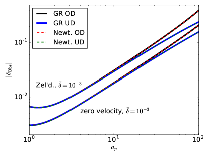
We first focus on simpler initial conditions of the form given by Eq. (9), where the inhomogeneities are initially all at a wavelength that is 4 times the initial Hubble radius, and follow the evolution of these inhomogeneities as they enter the horizon and grow. To begin with we compare a case where the initial velocity profile is zero to one where the velocity is given by the Zel’dovich approximation. In the latter case $|\delta_{N}|$ grows linearly with the scale factor in the Newtonian picture, beginning at the initial time. The zero-velocity initial data, on the other hand, includes both growing and decaying density perturbations, and so $|\delta_{N}|$ initially grows slower.

We show the density measured by some fiducial observers for these two cases in Fig. 1. Though the sizes of the initial Newtonian density perturbations $\delta_{N}$ are the same in both cases [given by Eq. (9) with $\bar{\delta}=10^{-3}$], they correspond to different densities through the relation given by Eq. (5). However, making use of this correspondence between the Newtonian and GR calculations, as illustrated in Fig. 1, both give fully consistent results, even as the perturbations become nonlinear—as evidenced by the diverging of the magnitude of the density contrast at the overdensities and underdensities. In what follows we will focus on initial conditions given by the Zel’dovich approximation velocity profile since this gives only growing modes, and we will study how close the relativistic and Newtonian calculations are in the nonlinear regime.

Figure 1: The density contrast as measured by an observer comoving with matter at the point of maximum overdensity (black and red curves) or underdensity (blue and green curves) for two cases with $\bar{\delta}=10^{-3}$ in Eq. (9), and an initial velocity profile that is either zero or given by the Zel’dovich approximation. The general-relativistic (solid lines) and Newtonian (dotted lines) calculations closely track each other.

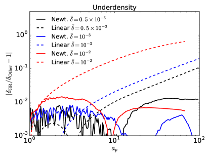
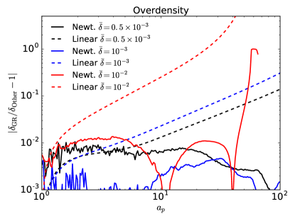
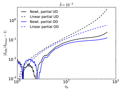
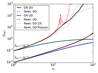
We can study how the difference between the calculations changes as a function of the magnitudes of the initial inhomogeneities. In Fig. 2 we again focus on the density measured by some fiducial observers and show the fractional difference between the GR and either Newtonian or linear perturbation results for a range of values for $\bar{\delta}$. For $\bar{\delta}\leq 10^{-3}$ a correction quadratic in $\bar{\delta}$ to the density is evident in the GR versus linear comparison, which reaches as high as tens of percent at the end. However, the difference from the Newtonian results is roughly an order of magnitude smaller. The $<1\%$ difference from this case seems to be consistent with being due to numerical truncation error, as illustrated in the Appendix. Since $|\psi_{N}|\lesssim 2\times 10^{-3}$ for these cases, even though the deviations from the background density are large, gravity is still weak.

Figure 2: The fractional difference between the density contrast $\delta_{\rm obs}$ at an underdensity (top) or overdensity (bottom) in the GR calculation compared to Newtonian simulations (solid lines) or linear perturbation theory (dotted lines) for various magnitudes of the initial inhomogeneities.

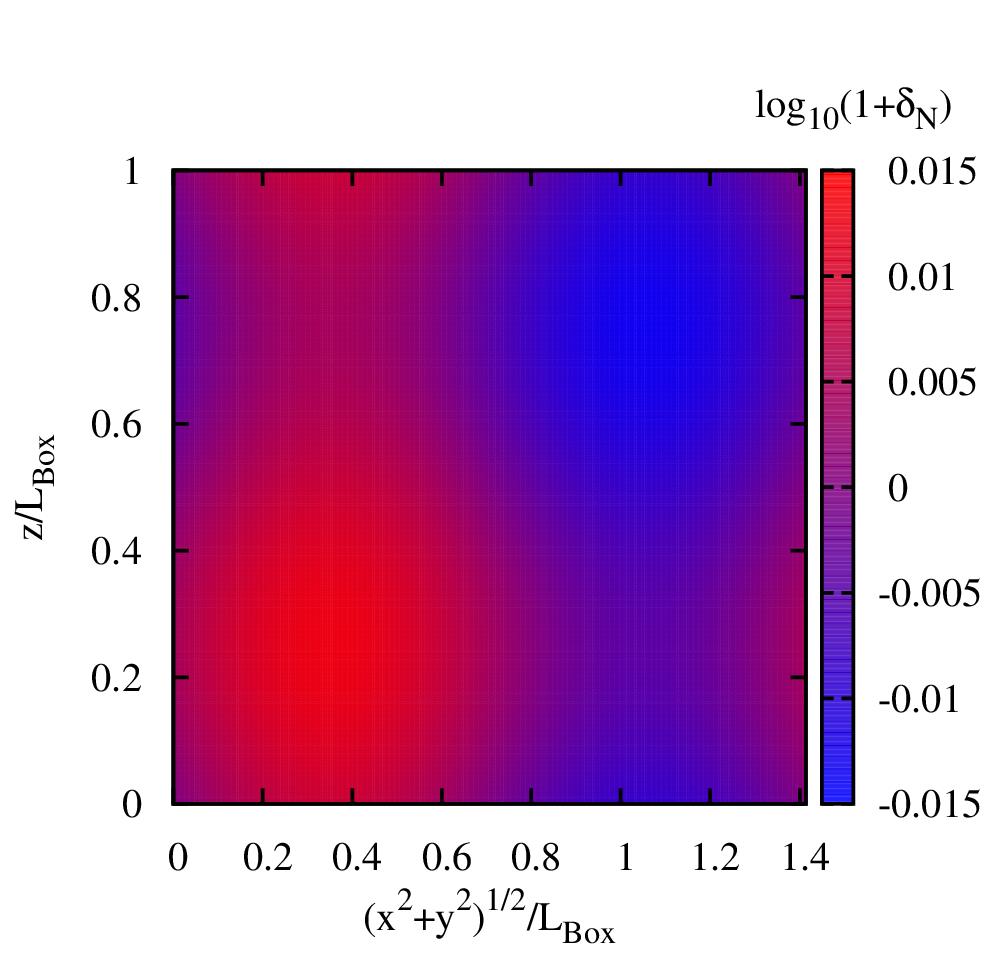
The case with $\bar{\delta}=10^{-2}$ is more extreme, with initial amplitude density perturbations that exceed the equivalent values in the standard $\Lambda$CDM model by roughly a factor of a 100. Figure 3 shows the initial and final density contrast $\delta_{N}$ from N-body simulations. Though the density at the point of maximum underdensity, which develops into a void, is again very close in the Newtonian and GR calculations, strong differences can be seen in the maximum overdensity at late times, with the Newtonian density exceeding that of the GR. In fact, in the Newtonian case a massive halo forms around this point with $\psi_{N}\sim-0.2$, while in the GR case the fluid density grows without bound, so the approximation of weak gravity is definitely breaking down. The divergence between the GR and Newtonian densities coincides quite well with the moment of halo formation predicted by the standard theory of spherical collapse, i.e. $a\approx 56$, at which the linearly extrapolated density contrast equals $1.686$. Before that, the GR and Newtonian simulations return fully consistent densities at all times until $a\approx 50$ when $\delta\approx 10$.

Figure 3: Two-dimensional slice of $\delta_{N}$ from the Newtonian simulations at the initial ($a=1$; top) and final ($a=60$; bottom) times from the $\bar{\delta}=10^{-2}$ case.

This discrepancy at halo formation is, of course, (at least partially) due to just the differing treatments of matter. In the particle case, after shell crossing at $a\approx 59$ at the point of maximum overdensity, the velocity dispersion goes from zero, to having a value of $\sigma_{v}\approx 0.2$–$0.3$. In the pressureless fluid treatment, there is nothing to halt the collapse, and we do not continue the calculation beyond this point. Thus, for this case we do not compare the GR and Newtonian results past the point where multistream regions form.

Similar but less extreme differences can also be found in other overdense and underdense regions in the $\bar{\delta}=10^{-2}$ case. As shown in Fig. 4, roughly $10\%$ differences appear at e.g. $(x,y,z)=(\pi/k)\times(-1/2,1/2,1/2)$ and $(\pi/k)\times(-1/2,-1/2,1/2)$ (and similarly at the permutations of the Cartesian directions). At both the overdense and underdense points shown, $|\delta_{\rm obs}|$ is larger in the Newtonian case. In contrast to the lower density cases, these differences do not appear to be due to resolution effects (though things do begin to become under-resolved at very late times at the center of the halo; see the Appendix for details).

Figure 4: The fractional difference between the density contrast $\delta_{\rm obs}$ measured by an observer comoving with the fluid initially at $(x,y,z)=(\pi/k)\times(-1/2,1/2,1/2)$ (black lines) and $(\pi/k)\times(-1/2,-1/2,1/2)$ (blue lines) in the GR calculation compared to Newtonian simulations (solid lines) or linear perturbation theory (dotted lines) for $\bar{\delta}=10^{-2}$.

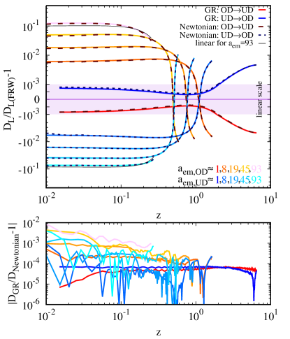
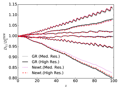
We can also compare the propagation of light as a measure of the differences between the two cases. To illustrate this, we note that our setup has a line of symmetry connecting the point of maximum overdensity and underdensity along which null geodesics will propagate. Hence, we can consider beams of light rays emitted by an observer at the overdensity (underdensity) at specified intervals of proper time and specified frequency, and calculate the redshift and luminosity distance, as seen by observers comoving with matter, as the beam propagates and finally reaches the underdensity (overdensity). This is shown in Figs. 5 and 6 for initial conditions with $\bar{\delta}=10^{-3}$ and $10^{-2}$, respectively. In the former we can see that, similar to the density contrast, at later times, once the perturbations have entered the horizon and begun collapsing, there are significant, order $10\%$, deviations from the homogeneous value of $D_{L}$, and also noticeable nonlinear corrections. However, again, the Newtonian and GR calculations agree quite well, with differences $\lesssim 1\%$, compatible with being due to numerical error.

Figure 5: The luminosity distance to the global maximum (OD) or minimum (UD) of the density field in the model with $\bar{\delta}=10^{-3}$. Distances are computed for an ensemble of observers located along the line joining the two critical points. Approximate values of the scale factor at subsequent moments of light emission are provided in the bottom right corner. The upper panel shows deviation of the GR/Newtonian distances from the corresponding observable based on the FRW metric and the bottom panel shows the fractional difference between the GR and Newtonian calculations. The shaded band indicates a linear scale of the vertical axis. The general-relativistic (thick solid lines) and Newtonian (dashed lines) simulations return consistent distances with compatible deviations from the FRW model and the predictions of linear Newtonian evolution (thin black lines, shown only for the latest emission time).

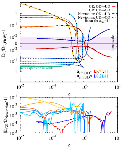
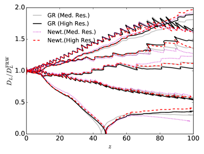
For the $\bar{\delta}=10^{-2}$ case shown in Fig. 6, there are even stronger effects from the inhomogeneities, with order unity deviations away from the linear perturbation value for $D_{L}$, and also some cases where the light rays are blueshifted as they approach the large, collapsing overdensity, causing $z$ to decrease. Again, the nonlinear Newtonian and GR calculations track each other quite well. However, there are noticeable differences which can be likely ascribed to the violation of the weak field regime, inside the halo of the Newtonian simulation (see the cases demonstrating light propagation inside the overdensity at late times: the yellow curve at small redshifts and the light blue curve at high redshifts).

Figure 6 demonstrates how the nonlinear phase of evolution, both in GR and Newtonian simulations, develops asymmetry between light propagation inside the overdensity and underdensity. For the latter, both simulations consistently show the emergence of a super-Hubble flow—a linear relation between redshift and distance with the effective Hubble constant $H_{\rm eff}>H_{0}$ at $z\lesssim 0.2$. Homogeneity of the super-Hubble expansion (in contrast to the local Hubble flow at the overdensity) reflects the fact that matter evacuation not only increases the density contrast in voids but also homogenizes the residual matter distribution (Wojtak et al., 2016). Our results demonstrate that both GR and Newtonian simulations provide a consistent description of this mechanism. In addition, we can see that the effective Hubble constant $H_{\rm eff}$ at subsequent emission times converges to its asymptotic value given by the maximum expansion in voids predicted in Newtonian gravity (the green line in Fig. 6), i.e. $H_{\rm eff}\rightarrow(3/2)H$ for $\Omega_{\rm m}=1$ (Bernardeau et al., 1997).

Figure 6: The same as Fig. 5 but for the case with $\bar{\delta}=10^{-2}$. The green line shows the maximum super-Hubble flow in empty voids, i.e. $\delta_{N}\rightarrow-1$, based on Newtonian calculations.

IV.2 Initial conditions with range of scales

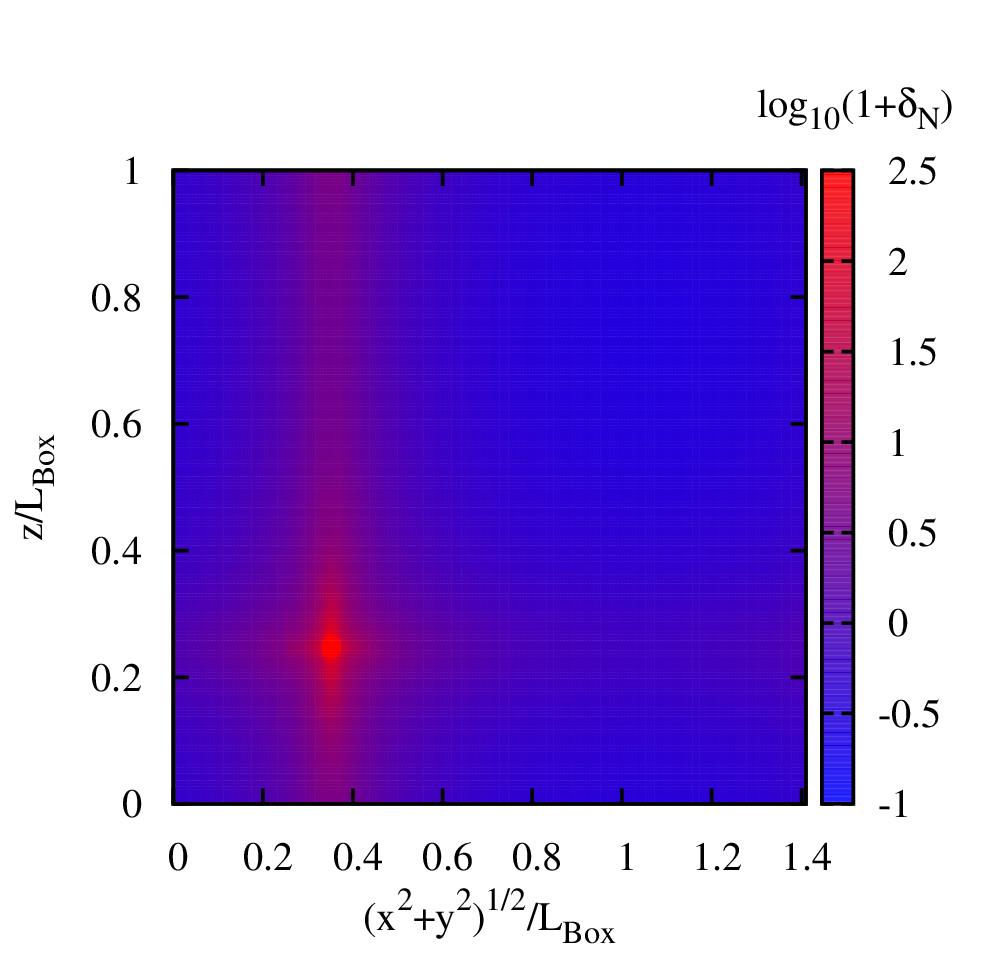
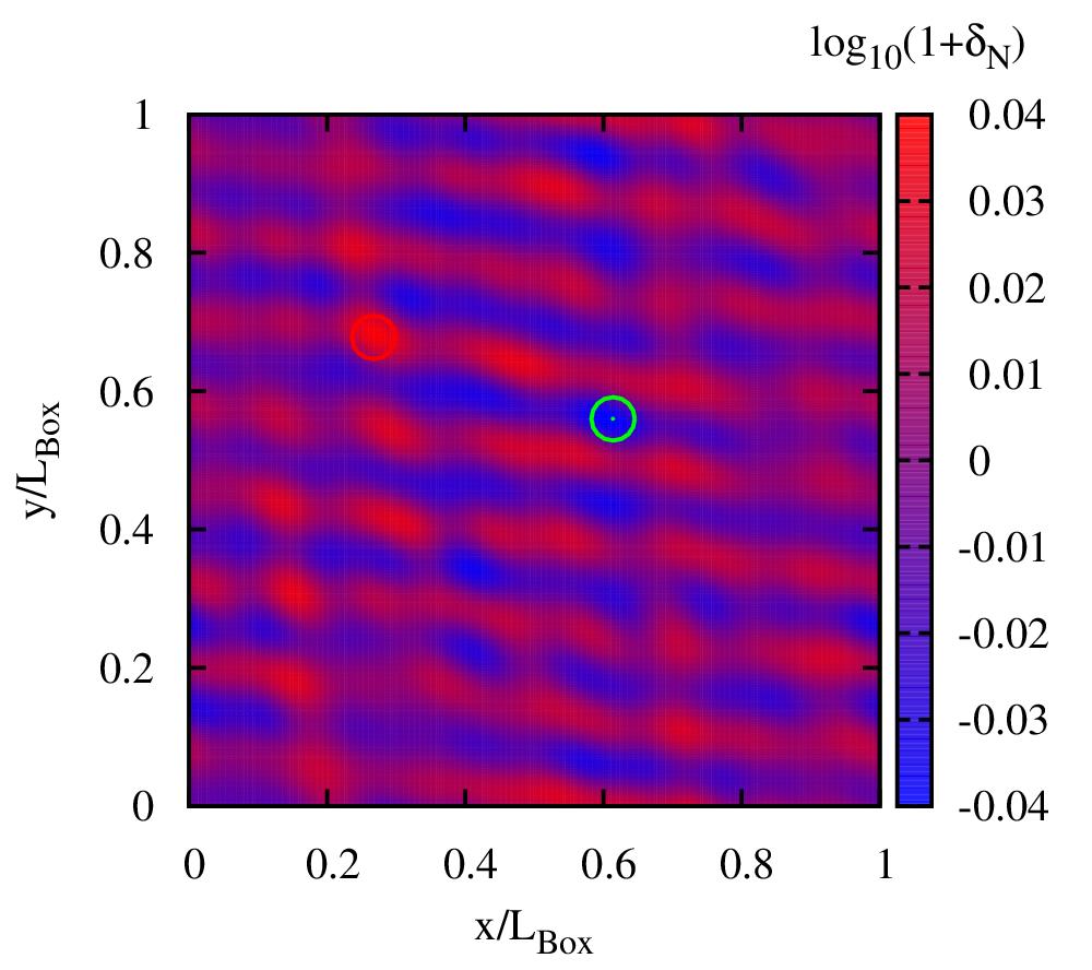
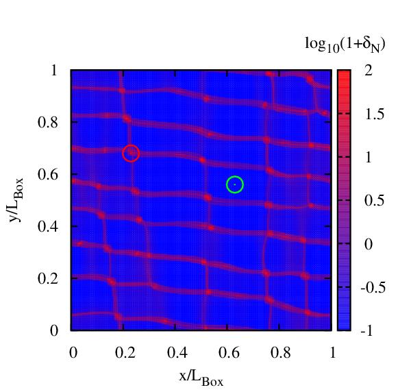
We next consider more general initial conditions that begin with variations over a range of length scales, to further study possible coupling between short and long length scales. In particular, we use the power spectrum initial conditions described in Sec. III.6 which have density variations on wavelengths ranging from 4 times to one-third the initial Hubble radius at two different amplitudes, which we label $\bar{\delta}_{\rm PS}=10^{-3}$ and $\bar{\delta}_{\rm PS}=10^{-2}$. To illustrate this we show a slice through the initial and final Newtonian density contrast from the higher amplitude case in Fig. 7. As is evident in the bottom panel, this model generates a network of halos with $\delta_{N}\gtrsim 10^{2}$ and voids with $\delta_{N}\sim-0.9$.

Figure 7: Two-dimensional slice of $\delta_{N}$ from the Newtonian simulations at the initial ($a=1$; top) and final ($a=100$; bottom) times from the $\bar{\delta}_{\rm PS}=10^{-2}$ case. The red and green points indicate the positions of fiducial observers initially at points of maximum overdensity and underdensity, respectively.

As an indication of the evolution of these cases, in Fig. 8 we show the density (relative to a FRW solution) seen by fiducial observers comoving with matter, at the initial points of minimum and maximum density (marked in Fig. 7). As in the previous cases, there is broad agreement between the Newtonian and GR results even as the inhomogeneities become large. At the point of maximum density, the velocity dispersion becomes nonzero in the particle case at $a\approx 15$ and eventually reaches a value of $\sigma_{v}\sim 0.04$. As nonlinear structure and multistream regions (in the N-body case) form, the density value at the overdensity becomes noisy, as well as fairly sensitive to resolution and the density estimator used. We illustrate this latter point in Fig. 8 by also including the density estimate for one of the N-body cases using two alternative methods: the cloud-in-cell method Springel (2005), and by calculating the density from the gravitational potential through the Poisson equation. Because of this, in what follows we will concentrate on comparing the propagation of light rays in the respective spacetimes.

Figure 8: The density contrast as measured by an observer comoving with matter at the points of maximum overdensity (black and red curves) and underdensity (blue and green curves) shown in Fig. 7 for two cases with $\bar{\delta}_{\rm PS}=10^{-3}$ and $\bar{\delta}_{\rm PS}=10^{-2}$. The general-relativistic (solid lines) and Newtonian (dashed lines) calculations closely track each other except at the overdensity in the largest amplitude case where a noisy multistream region forms. In such regions the N-body density contrast is sensitive to the particular density estimator used, which we illustrate by also including the cloud-in-cell density estimate, as well as the one obtained from the potential through the Poisson equation (dotted lines), for one case.

Since it does not have the discrete symmetry of the initial conditions considered in Sec. IV.1, for this setup we consider a set of light rays with initial positions at the points of minimum and maximum density, as well as an intermediate point with $\delta_{N}=0$. For each position we consider light rays with initial velocities pointing in plus and minus each of the $x$, $y$, and $z$ coordinate directions that then propagate throughout the simulations. We show the luminosity-redshift values—again, as measured by observers comoving with matter—for a representative set of these in Fig. 9 for $\bar{\delta}_{\rm PS}=10^{-3}$ and Fig. 10 for $\bar{\delta}_{\rm PS}=10^{-3}$. The effect of short and longer wavelength inhomogeneities is evident in higher and lower frequency components of the deviations from the homogeneous values of $D_{L}$ versus $z$. In the higher amplitude case (Fig. 10) strongly nonlinear effects are apparent, including instances of decreasing redshift with increasing luminosity distance and “lensing” which causes $D_{L}$ to pass through zero. However, these features are captured by both the full GR spacetime and the one reconstructed from the Newtonian solution. Though there are some evident quantitative differences between the values of $D_{L}$ obtained in the two cases, these can be primarily attributed to numerical truncation error due to the small-scale structure eventually not being well resolved. This is illustrated in the Appendix (in particular, Fig. 14), where we include lower resolution results.

Figure 9: The luminosity distance to the global minimum (left panels), the node point (middle panels) and the global maximum (right panels) of the initial density field in the cosmological model with $\bar{\delta}_{\rm PS}=10^{-3}$. Distances are computed for observers located along photon rays emitted at the scale factor $a_{\rm em}=1$ in the $x$, $y$ and $z$ directions. The upper panels show deviations between the GR and Newtonian distances from the corresponding observables based on the unperturbed FRW metric, and the bottom panels show the fractional difference between the GR and Newtonian results. Both the GR and Newtonian simulations return consistent distances with nearly the same deviations from the FRW model.

Figure 10: The same as Fig. 9 but for the case with $\bar{\delta}_{\rm PS}=10^{-2}$. The fractional differences are computed at the same value of affine parameters and plotted as a function of redshift from the GR simulations. The corresponding fractional differences in redshift are smaller than $10^{-2}$ at all times.

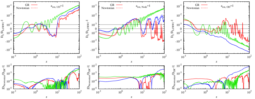
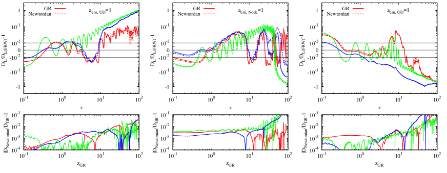
Figures 9 and 10 clearly demonstrate a difference between light propagating primarily in voids (left panels) or overdense regions (right panels). The cumulative effect of tidal forces (corresponding to the Riemann tensor in the GR calculations) makes the photon rays diverge in the former case or converge in the latter. This in turn manifests itself as demagnification (increased distances) or magnification (decreased distances), respectively. Our results show that this cumulative lensing effect is consistently described both in fully GR computations and in (relativistic) ray tracing on the effective spacetime of the Newtonian simulations.

V Discussion and Conclusion

We have systematically compared cosmological models of structure formation calculated using the full Einstein equations, to those using Newtonian gravity on a homogeneously expanding background. We considered a suite of globally flat cold dark matter models (Einstein–de Sitter models) with a range of density perturbations on scales comparable to the Hubble horizon at the initial time. Starting with consistent initial conditions based on the correspondence between GR and Newtonian cosmology in the linear regime of the density evolution, we evolved the models to a highly nonlinear phase using both numerical GR coupled to hydrodynamics and N-body techniques. The GR and Newtonian simulations were then compared in terms of the density field and the properties of light propagation. The former was consistently calculated for an ensemble of freely falling observers located at various points of the initial density field. The latter was quantified by solving the geodesic equations describing bundles of light rays emitted from a set of sources, consistently defined in both simulations. Every bundle of geodesics was then used to determine cosmological distance as a function of redshift, as measured by free-falling observers located along the photon path.

Our comparison between GR and Newtonian simulations in the highly nonlinear phase does not reveal any significant differences, as long as the Newtonian potential does not violate the weak field assumption. Our resolution studies show that in most cases any apparent differences between the GR densities and their counterparts from Newtonian simulations—typically sub-percent in the level of the inhomogeneities—are due to truncation error in the simulations. In general, the fractional differences between the two decrease in higher resolution runs. The only exception is one case with high density regions with shell crossings. In this one case, we were not able to continue the GR fluid calculation past the time where shell crossing occurs in the Newtonian N-body calculation. This is predominantly due to the lack of full conformity between the treatment of matter in the hydrodynamical and particle description. A more thorough comparison of GR and Newtonian simulations into this regime will probably require using particles (or hydrodynamics) with both treatments of gravity. In the other cases considered here, particle versus fluid differences due to multistream regions were subdominant to numerical truncation error.

Despite some noticeable differences between GR and Newtonian in regions where the weak gravity assumption is violated, we do not see any dissimilarities between gravitational collapse in the GR and Newtonian frameworks. In particular, in the model with the highest amplitude of the initial density field ($\bar{\delta}=10^{-2}$), the Newtonian evolution closely resembles the GR collapse until $\delta_{\rm N}\sim 10$. Taking the moment of abrupt growth of density as the halo formation time (the first shell crossing in Newtonian simulations), we demonstrated that both GR and Newtonian simulations point to the halo formation time that is consistent with the standard spherical collapse model. This is in contrast to (Bentivegna and Bruni, 2016) which considered a similar setup, and reported a lag between gravitational collapse in GR and the standard (Newtonian) spherical model. Our study also suggests that the results of Giblin et al. (2016a, b) are similarly in a regime where the observed nonlinear effects should be well captured by a nonlinear Newtonian calculation.

In our study we have made use of the “abridged dictionary” of Chisari and Zaldarriaga (2011); Green and Wald (2012) which relates the quantities from a Newtonian cosmology calculation to the general-relativistic spacetime metric and stress-energy tensor that they should approximate. Though this correspondence is only strictly applicable at the linear level, as argued in Green and Wald (2012), the corrections should be small even with large inhomogeneities, as long as they occur on small scales and the gravitational potential remains small. Our study demonstrates, for the first time, by means of explicit comparison of fully GR and Newtonian cosmological simulations, that indeed this is the case, even beginning with inhomogeneities on scales comparable to the Hubble horizon and continuing to the highly nonlinear regime of the density evolution. The Newtonian simulations are able to arrive at these solutions with considerably less computational expense, both because of the fewer number and less complicated nature of evolution equations and because roughly 100 times fewer time steps have to be taken. In most cases, we found the differences between the Newtonian and relativistic calculations to be dominated simply by numerical errors. Though here we focused on somewhat simplified setups with a limited range of length scales, and hence less stringent resolution requirements, production-level structure-formation N-body simulations typically have numerical errors that are comparable or worse Heitmann et al. (2008); Schneider et al. (2016), meaning it will be quite challenging to make such errors subdominant to any relativistic effects. Having said that, we emphasize that we have focused on somewhat simplified setups in this work, and our study does not exhaust all possible initial conditions, nor probe the effects of other types of matter or cosmological parameters such as dark energy, curvature, etc. Other, more relativistic types of matter, e.g. neutrinos, may exhibit stronger differences.

The close resemblance between our GR and Newtonian simulations is especially prominent in the comparison distances calculated from ray tracing (in both cases, based on solving geodesic equations describing bundles of light rays). Both simulations consistently capture all effects, giving rise to noticeable deviations from the observables based on the FRW metric including the enhanced (suppressed) expansion in overdense (underdense) regions (see Figs. 5 and 6) and the demagnification (magnification) in voids (overdensities) (see Figs. 9 and 10). Although numerical errors appear to be larger for some cases featuring particularly strong lensing, ray tracing yields remarkably similar characterization of these lensing events in both simulations.

Most observables used in cosmological inference are not based on directly integrating the geodesic equation but are rather derived under a number of simplifying assumptions, e.g. linearity of density evolution and the Born approximation of thin lenses adopted commonly in lensing calculations. However, it is not obvious whether forgoing such approximations when calculating observables can introduce significant corrections or not, and this is something currently under investigation (e.g. Petri et al. (2017); Fabbian et al. (2017)). Several recent studies have attempted to address this problem by combining fully GR cosmological simulations with full ray tracing (Giblin et al., 2016b, 2017). Our results suggest, however, that any possible corrections to the standard cosmological observables may stem from inaccurate ray tracing adopted in the standard framework rather than from a genuine difference between GR and Newtonian evolution of the density field. Therefore, to test the standard framework for calculating cosmological observables, it may be worth further exploring the easier and computationally less expensive strategy of using standard N-body simulations to reconstruct a spacetime and directly integrating geodesics on it, as we do here (see Koksbang and Hannestad (2015a, b) for work along these lines). The same strategy can also be useful in theoretical considerations involving cosmological models with large-scale perturbations exceeding the limits imposed by the standard $\Lambda$CDM model. For example, our study shows that models with large-scale local voids can feature substantially higher, locally measured, Hubble constants and thus are able to reproduce basic properties of recently studied cosmological models with an observationally constrained relation between the cosmological redshift and cosmic scale factor, dubbed redshift remapping (Wojtak and Prada, 2016, 2017).

Appendix: Numerical error results

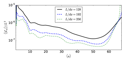
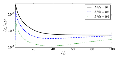
In this appendix we give some details on numerical convergence and error estimates. It is important to determine if the differences seen between the various quantities compared between the Newtonian and GR simulations are due to the differences in the underlying equations or just to differences in the numerical truncation error. In order to estimate this, we run selected cases at multiple resolutions. For the Newtonian N-body simulations we use a low, medium, and high resolution with $64^{3}$, $128^{3}$, and $256^{3}$ particles, respectively. For most of the GR calculations we use a low, medium, and high resolution with a grid with $96^{3}$, $128^{3}$, and $192^{3}$ cells, respectively. For the cases with the largest amplitude inhomogeneities (the $\bar{\delta}=10^{-2}$ and $\bar{\delta}_{\rm PS}=10^{-2}$ cases) we use $128^{3}$, $192^{3}$, and $256^{3}$ grid cells. To illustrate convergence, in Fig. 11 we show the magnitude of the generalized harmonic constraint violation for several cases. The convergence of this quantity to zero with increasing resolution is a nontrivial check that the constraint equations at the initial time, and the evolution equations, are being solved with sufficient resolution (see Pretorius (2005)).

Figure 11: The volume average of the norm of the constraint violation $\mathcal{C}_{a}:=\Box x_{a}-H_{a}$ as a function time (parametrized by a volume-averaged measure of the effective scale factor), for simulations with $\bar{\delta}=10^{-2}$ (top) and $\bar{\delta}_{\rm PS}=10^{-3}$ (bottom) at three different resolutions. The decrease in constraint violation with increasing resolution is consistent with roughly second-order convergence.

The Newtonian and GR calculations will have different truncation error, with different dependence on resolution. However, to give a rough estimate, we show the difference between several quantities in the Newtonian and GR simulations at multiple resolutions. In Fig. 12 we show the difference in the density contrast measured at the overdensity and underdensity for $\bar{\delta}=10^{-3}$ and $\bar{\delta}=10^{-2}$ (left and middle panels; cf. Fig. 2), as well as some intermediate points for $\bar{\delta}=10^{-2}$ (right panel; cf. Fig. 4). For many of the cases, the difference between the two calculations decreases as the resolution of the respective simulations is increased, indicating that the discrepancy is primarily attributable to truncation error. However, at late times in several of the $\bar{\delta}=10^{-2}$ cases, differences in the density that are consistent with increasing resolution are apparent.

Figure 12: The relative difference in density contrast $\delta_{\rm obs}$ between the GR and Newtonian simulations, at three different sets of resolutions. The left and middle panels show the points of maximum overdensity and underdensity for $\bar{\delta}=10^{-3}$ and $\bar{\delta}=10^{-2}$, respectively (similar to Fig. 2), while the right panel shows the same intermediate points from the $\bar{\delta}=10^{-2}$ case as in Fig. 4.

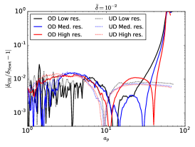
We also show the dependency of the redshift-luminosity relations on resolution in Fig. 13. Again, for the $\bar{\delta}=10^{-3}$ case shown in the top panel, the difference between the GR and Newtonian results decreases noticeably with increasing resolution, indicating that the $\lesssim 1\%$ differences seen in Fig. 5 are likely dominated by truncation error. Here we just show the light rays beginning at the overdensity and ending at the underdensity, but the reverse ones are similar. However, for the $\bar{\delta}=10^{-2}$ case shown in the bottom panel, there are some significant differences in the luminosity distance in the vicinity of the overdensity as it collapses at later times, though the differences diminish as the light rays propagate farther away.

Figure 13: The relative difference in the luminosity versus redshift between the GR and Newtonian simulations at different resolutions for light rays emitted at the point of maximum overdensity that propagate to the point of maximum underdensity for the $\bar{\delta}=10^{-3}$ (top) and $\bar{\delta}=10^{-2}$ (bottom) cases, similar to Figs. 5 and 6.

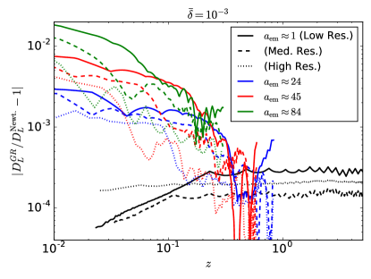
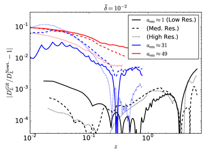
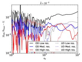
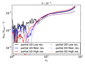
Finally, as an indication of the magnitude of truncation error in the power-spectrum initial conditions simulations, in Fig. 14 we show high- and medium-resolution results for redshift versus luminosity for $\bar{\delta}_{\rm PS}=10^{-3}$ and $\bar{\delta}_{\rm PS}=10^{-2}$. Here it can be seen that the difference between the GR and Newtonian values is both comparable to the difference with resolution and diminishes as the resolution is increased. This is true both for $\bar{\delta}_{\rm PS}=10^{-3}$ (top panel), where the differences are small, and $\bar{\delta}_{\rm PS}=10^{-2}$ (bottom panel), where stronger resolution-dependent effects are evident at late times.

Figure 14: The luminosity distance (normalized by the FRW value) versus redshift for a representative set of null rays in the $\bar{\delta}_{\rm PS}=10^{-3}$ (top) and $\bar{\delta}_{\rm PS}=10^{-2}$ (bottom) cases. We show results from both the highest resolution GR (solid black lines) and Newtonian (dashed red lines) simulations, as well as lower resolution results from both cases (grey solid and magenta dashed lines, for GR and Newtonian, respectively) to indicate the magnitude of the numerical truncation error.

References

- Bentivegna and Bruni (2016) E. Bentivegna and M. Bruni, Phys. Rev. Lett. 116, 251302 (2016), arXiv:1511.05124 [gr-qc] .
- Giblin et al. (2016a) J. T. Giblin, J. B. Mertens, and G. D. Starkman, Phys. Rev. Lett. 116, 251301 (2016a), arXiv:1511.01105 [gr-qc] .
- Giblin et al. (2016b) J. T. Giblin, J. B. Mertens, and G. D. Starkman, Astrophys. J. 833, 247 (2016b), arXiv:1608.04403 [astro-ph.CO] .
- Macpherson et al. (2017) H. J. Macpherson, P. D. Lasky, and D. J. Price, Phys. Rev. D95, 064028 (2017), arXiv:1611.05447 [astro-ph.CO] .
- Daverio et al. (2016) D. Daverio, Y. Dirian, and E. Mitsou, (2016), arXiv:1611.03437 [gr-qc] .
- Buchert (2000) T. Buchert, Gen. Rel. Grav. 32, 105 (2000), arXiv:gr-qc/9906015 [gr-qc] .
- Kolb et al. (2005) E. W. Kolb, S. Matarrese, A. Notari, and A. Riotto, Phys. Rev. D71, 023524 (2005), arXiv:hep-ph/0409038 [hep-ph] .
- Rasanen (2011) S. Rasanen, Class. Quant. Grav. 28, 164008 (2011), arXiv:1102.0408 [astro-ph.CO] .
- Ishibashi and Wald (2006) A. Ishibashi and R. M. Wald, Class. Quant. Grav. 23, 235 (2006), arXiv:gr-qc/0509108 [gr-qc] .
- Green and Wald (2014) S. R. Green and R. M. Wald, Class. Quant. Grav. 31, 234003 (2014), arXiv:1407.8084 [gr-qc] .
- Collaboration (2017) D. Collaboration, ArXiv e-prints (2017), arXiv:1708.01530 .
- Levi et al. (2013) M. Levi, C. Bebek, T. Beers, R. Blum, R. Cahn, D. Eisenstein, B. Flaugher, K. Honscheid, R. Kron, O. Lahav, P. McDonald, N. Roe, D. Schlegel, and representing the DESI collaboration, ArXiv e-prints (2013), arXiv:1308.0847 [astro-ph.CO] .
- LSST Dark Energy Science Collaboration (2012) LSST Dark Energy Science Collaboration, ArXiv e-prints (2012), arXiv:1211.0310 [astro-ph.CO] .
- Laureijs et al. (2011) R. Laureijs, J. Amiaux, S. Arduini, J. . Auguères, J. Brinchmann, R. Cole, M. Cropper, C. Dabin, L. Duvet, A. Ealet, and et al., ArXiv e-prints (2011), arXiv:1110.3193 [astro-ph.CO] .
- Keenan et al. (2013) R. C. Keenan, A. J. Barger, and L. L. Cowie, Astrophys. J. 775, 62 (2013), arXiv:1304.2884 [astro-ph.CO] .
- Böhringer et al. (2015) H. Böhringer, G. Chon, M. Bristow, and C. A. Collins, Astron. Astrophys. 574, A26 (2015), arXiv:1410.2172 .
- Chisari and Zaldarriaga (2011) N. E. Chisari and M. Zaldarriaga, Phys. Rev. D83, 123505 (2011), [Erratum: Phys. Rev.D84,089901(2011)], arXiv:1101.3555 [astro-ph.CO] .
- Green and Wald (2012) S. R. Green and R. M. Wald, Phys. Rev. D85, 063512 (2012), arXiv:1111.2997 [gr-qc] .
- Abel et al. (2012) T. Abel, O. Hahn, and R. Kaehler, Mon. Not. R. Astron. Soc. 427, 61 (2012), arXiv:1111.3944 .
- Beyer and Sarbach (2004) H. R. Beyer and O. Sarbach, Phys. Rev. D70, 104004 (2004), arXiv:gr-qc/0406003 [gr-qc] .
- Alonso et al. (2010) D. Alonso, J. Garcia-Bellido, T. Haugbolle, and J. Vicente, Phys. Rev. D82, 123530 (2010), arXiv:1010.3453 [astro-ph.CO] .
- Adamek et al. (2016) J. Adamek, D. Daverio, R. Durrer, and M. Kunz, Nature Phys. 12, 346 (2016), arXiv:1509.01699 [astro-ph.CO] .
- Adamek et al. (2017) J. Adamek, R. Durrer, and M. Kunz, (2017), arXiv:1707.06938 [astro-ph.CO] .
- Hahn and Paranjape (2016) O. Hahn and A. Paranjape, Phys. Rev. D 94, 083511 (2016), arXiv:1602.07699 .
- Bentivegna and Korzynski (2012) E. Bentivegna and M. Korzynski, Class. Quant. Grav. 29, 165007 (2012), arXiv:1204.3568 [gr-qc] .
- Yoo et al. (2013) C.-M. Yoo, H. Okawa, and K.-i. Nakao, Phys. Rev. Lett. 111, 161102 (2013), arXiv:1306.1389 [gr-qc] .
- Yoo and Okawa (2014) C.-M. Yoo and H. Okawa, Phys. Rev. D89, 123502 (2014), arXiv:1404.1435 [gr-qc] .
- Bruni et al. (2014) M. Bruni, D. B. Thomas, and D. Wands, Phys. Rev. D89, 044010 (2014), arXiv:1306.1562 [astro-ph.CO] .
- Thomas et al. (2015) D. B. Thomas, M. Bruni, and D. Wands, Mon. Not. Roy. Astron. Soc. 452, 1727 (2015), arXiv:1501.00799 [astro-ph.CO] .
- Zel’dovich (1970) Y. B. Zel’dovich, Astron. Astrophys. 5, 84 (1970).
- East et al. (2012a) W. E. East, F. M. Ramazanoglu, and F. Pretorius, Phys. Rev. D86, 104053 (2012a), arXiv:1208.3473 [gr-qc] .
- Springel (2005) V. Springel, Mon. Not. R. Astron. Soc. 364, 1105 (2005), astro-ph/0505010 .
- Shandarin et al. (2012) S. Shandarin, S. Habib, and K. Heitmann, Phys. Rev. D 85, 083005 (2012), arXiv:1111.2366 .
- East et al. (2012b) W. E. East, F. Pretorius, and B. C. Stephens, Phys.Rev. D85, 124010 (2012b), arXiv:1112.3094 [gr-qc] .
- Choptuik and Pretorius (2010) M. W. Choptuik and F. Pretorius, Phys. Rev. Lett. 104, 111101 (2010), arXiv:0908.1780 [gr-qc] .
- Lindblom and Szilágyi (2009) L. Lindblom and B. Szilágyi, Phys. Rev. D 80, 084019 (2009), arXiv:0904.4873 [gr-qc] .
- East et al. (2016) W. E. East, M. Kleban, A. Linde, and L. Senatore, JCAP 1609, 010 (2016), arXiv:1511.05143 [hep-th] .
- Bentivegna et al. (2017) E. Bentivegna, M. Korzyński, I. Hinder, and D. Gerlicher, JCAP 1703, 014 (2017), arXiv:1611.09275 [gr-qc] .
- Etherington (2007) I. M. H. Etherington, General Relativity and Gravitation 39, 1055 (2007).
- Perlick (2004) V. Perlick, Living Reviews in Relativity 7, 9 (2004).
- Wojtak et al. (2016) R. Wojtak, D. Powell, and T. Abel, Mon. Not. R. Astron. Soc. 458, 4431 (2016), arXiv:1602.08541 .
- Bernardeau et al. (1997) F. Bernardeau, R. van de Weygaert, E. Hivon, and F. R. Bouchet, Mon. Not. R. Astron. Soc. 290, 566 (1997), astro-ph/9609027 .
- Heitmann et al. (2008) K. Heitmann et al., Comput. Sci. Dis. 1, 015003 (2008), arXiv:0706.1270 [astro-ph] .
- Schneider et al. (2016) A. Schneider, R. Teyssier, D. Potter, J. Stadel, J. Onions, D. S. Reed, R. E. Smith, V. Springel, F. R. Pearce, and R. Scoccimarro, JCAP 1604, 047 (2016), arXiv:1503.05920 [astro-ph.CO] .
- Petri et al. (2017) A. Petri, Z. Haiman, and M. May, Phys. Rev. D95, 123503 (2017), arXiv:1612.00852 [astro-ph.CO] .
- Fabbian et al. (2017) G. Fabbian, M. Calabrese, and C. Carbone, (2017), arXiv:1702.03317 [astro-ph.CO] .
- Giblin et al. (2017) J. T. Giblin, Jr, J. B. Mertens, G. D. Starkman, and A. R. Zentner, ArXiv e-prints (2017), arXiv:1707.06640 .
- Koksbang and Hannestad (2015a) S. M. Koksbang and S. Hannestad, Phys. Rev. D91, 043508 (2015a), arXiv:1501.01413 [astro-ph.CO] .
- Koksbang and Hannestad (2015b) S. M. Koksbang and S. Hannestad, Phys. Rev. D92, 023532 (2015b), [Erratum: Phys. Rev.D92,no.6,069904(2015)], arXiv:1506.09127 [astro-ph.CO] .
- Wojtak and Prada (2016) R. Wojtak and F. Prada, Mon. Not. R. Astron. Soc. 458, 3331 (2016), arXiv:1602.02231 .
- Wojtak and Prada (2017) R. Wojtak and F. Prada, Mon. Not. R. Astron. Soc. 470, 4493 (2017), arXiv:1610.03599 .
- Pretorius (2005) F. Pretorius, Class. Quantum Grav. 22, 425 (2005), arXiv:gr-qc/0407110 .