Frobenius-Perron theory of endofunctors

Abstract.

We introduce the Frobenius-Perron dimension of an endofunctor of a $\Bbbk$-linear category and provide some applications.

0. Introduction

The spectral radius (also called the Frobenius-Perron dimension) of a matrix is an elementary and extremely useful invariant in linear algebra, combinatorics, topology, probability and statistics. The Frobenius-Perron dimension has become a crucial concept in the study of fusion categories and representations of semismiple weak Hopf algebras since it was introduced by Etingof-Nikshych-Ostrik [ENO] in early 2000 (also see [EG, EGO, Ni]). In this paper several Frobenius-Perron type invariants are proposed to study derived categories, representations of finite dimensional algebras, and complexity of algebras and categories.

Throughout let $\Bbbk$ be an algebraically closed field, and let everything be over $\Bbbk$.

0.1. Definitions

The first goal is to introduce the Frobenius-Perron dimension of an endofunctor of a category. If an object $V$ in a fusion category ${\mathcal{C}}$ is considered as the associated tensor endofunctor $V\otimes_{\mathcal{C}}-$, then our definition of the Frobenius-Perron dimension agrees with the definition given in [ENO], see [Example 2.11] for details. Our definition applies to the derived category of projective schemes and finite dimensional algebras, as well as other abelian and additive categories [Definitions 2.3 and 2.4]. We refer the reader to Section 2 for the following invariants of an endofunctor:

1. Frobenius-Perron dimension (denoted by $\operatorname{fpd}$, and $\operatorname{fpd}^{n}$ for $n\geq 1$),

2. Frobenius-Perron growth (denoted by $\operatorname{fpg}$),

3. Frobenius-Perron curvature (denoted by $\operatorname{fpv}$), and

4. Frobenius-Perron series (denoted by $\operatorname{FP}$).

One can further define the above invariants for an abelian or a triangulated category. Note that the Frobenius-Perron dimension/growth/curvature of a category can be a non-integer, see Proposition 5.12(1), Example 8.7, and Remark 5.13(5) for non-integral values of $\operatorname{fpd}$, $\operatorname{fpg}$, and $\operatorname{fpv}$ respectively.

If ${\mathfrak{A}}$ is an abelian category, let $D^{b}({\mathfrak{A}})$ denote the bounded derived category of ${\mathfrak{A}}$. On the one hand it is reasonable to call $\operatorname{fpd}$ a dimension function since

$$\operatorname{fpd}(D^{b}(\operatorname{Mod}-\Bbbk[x_{1},\cdots,x_{n}]))=n$$

[Proposition 4.3(1)], but on the other hand, one might argue that $\operatorname{fpd}$ should not be called a dimension function since

$$\operatorname{fpd}(D^{b}(coh({\mathbb{P}}^{n})))=\begin{cases}1,&\quad n=1\\ \infty,&\quad n\geq 2\end{cases}$$

[Propositions 6.5 and 6.7]. In the latter case, $\operatorname{fpd}$ is an indicator of representation type of the category of $coh({\mathbb{P}}^{n})$, namely, $coh({\mathbb{P}}^{n})$ is tame if $n=1$, and is of wild representation type for all $n\geq 2$. A similar statement holds for projective curves in terms of genus [Proposition 6.5].

We can define the Frobenius-Perron (“fp”) version of several other classical invariants

1. fp global dimension (denoted by $\operatorname{fpgldim}$) [Definition 2.7(1)],

2. fp Kodaira dimension (denoted by $\textup{fp}\kappa$) [CG].

The first one is defined for all triangulated categories and the second one is defined for triangulated categories with Serre functor. In general, the $\operatorname{fpgldim}A$ does not agree with the classical global dimension of $A$ [Theorem 7.8]. The fp version of the Kodaira dimension agrees with the classical definition for smooth projective schemes [CG].

Our second goal is to provide several applications.

0.2. Embeddings

In addition to the fact that the Frobenius-Perron dimension is an effective and sensible invariant of many categories, this invariant increases when the “size” of the endofunctors and categories increase.

Theorem 0.1.

Suppose ${\mathcal{C}}$ and ${\mathcal{D}}$ are $\Bbbk$-linear categories. Let $F:{\mathcal{C}}\to{\mathcal{D}}$ be a fully faithful functor. Let $\sigma_{\mathcal{C}}$ and $\sigma_{\mathcal{D}}$ be endofunctors of ${\mathcal{C}}$ and ${\mathcal{D}}$ respectively. Suppose that $F\circ\sigma_{\mathcal{C}}$ is naturally isomorphic to $\sigma_{\mathcal{D}}\circ F$. Then $\operatorname{FP}(u,t,\sigma_{\mathcal{C}})\leq\operatorname{FP}(u,t,\sigma_{\mathcal{D}})$.

By taking $\sigma$ to be the suspension functor of a pre-triangulated category, we have the following immediate consequence. (Note that the fp-dimension of a triangulated category ${\mathcal{T}}$ is defined to be $\operatorname{fpd}(\Sigma)$, where $\Sigma$ is the suspension of ${\mathcal{T}}$.)

Corollary 0.2.

Let ${\mathcal{T}}_{2}$ be a pre-triangulated category and ${\mathcal{T}}_{1}$ a full pre-triangulated subcategory of ${\mathcal{T}}_{2}$. Then the following hold.

1. $\operatorname{fpd}{\mathcal{T}}_{1}\leq\operatorname{fpd}{\mathcal{T}}_{2}$.

2. $\operatorname{fpg}{\mathcal{T}}_{1}\leq\operatorname{fpg}{\mathcal{T}}_{2}$.

3. $\operatorname{fpv}{\mathcal{T}}_{1}\leq\operatorname{fpv}{\mathcal{T}}_{2}$.

4. If ${\mathcal{T}}_{2}$ has fp-subexponential growth, so does ${\mathcal{T}}_{1}$.

Fully faithful embeddings of derived categories of projective schemes have been investigated in the study of Fourier-Mukai transforms, birational geometry, and noncommutative crepant resolutions (NCCRs) by Bondal-Orlov [BO1, BO2], Van den Bergh [VdB], Bridgeland [Bri], Bridgeland-King-Reid [BKR] and more.

Note that if $\operatorname{fpgldim}({\mathcal{T}})<\infty$, then $\operatorname{fpg}({\mathcal{T}})=0$. If $\operatorname{fpg}({\mathcal{T}})<\infty$, then $\operatorname{fpv}({\mathcal{T}})\leq 1$. Hence, $\operatorname{fpd}$, $\operatorname{fpgldim}$, $\operatorname{fpg}$ and $\operatorname{fpv}$ measure the “size”, “representation type”, or “complexity” of a triangulated category ${\mathcal{T}}$ at different levels. Corollary 0.2 has many consequences concerning non-existence of fully faithful embeddings provided that we compute the invariants $\operatorname{fpd}$, $\operatorname{fpg}$ and $\operatorname{fpv}$ of various categories efficiently.

0.3. Tame vs wild

Here we mention a couple of more applications. First we extend the classical trichotomy on the representation types of quivers to the $\operatorname{fpd}$.

Theorem 0.3.

Let $Q$ be a finite quiver and let ${\mathcal{Q}}$ be the bounded derived category of finite dimensional left $\Bbbk Q$-modules.

1. $\Bbbk Q$ is of finite representation type if and only if $\operatorname{fpd}{\mathcal{Q}}=0$.

2. $\Bbbk Q$ is of tame representation type if and only if $\operatorname{fpd}{\mathcal{Q}}=1$.

3. $\Bbbk Q$ is of wild representation type if and only if $\operatorname{fpd}{\mathcal{Q}}=\infty$.

By the classical theorems of Gabriel [Ga1] and Nazarova [Na], the quivers of finite and tame representation types correspond to the $ADE$ and $\widetilde{A}\widetilde{D}\widetilde{E}$ diagrams respectively.

The above theorem fails for quiver algebras with relations [Proposition 5.12]. As we have already seen, $\operatorname{fpd}$ is related to the “size” of a triangulated category, as well as, the representation types. We will see soon that $\operatorname{fpg}$ is also closely connected with the complexity of representations. When we focus on the representation types, we make some tentative definitions.

Let ${\mathcal{T}}$ be a triangulated category (such as $D^{b}(\operatorname{Mod}_{f.d.}-A)$).

1. We call ${\mathcal{T}}$ fp-trivial, if $\operatorname{fpd}{\mathcal{T}}=0$.

2. We call ${\mathcal{T}}$ fp-tame, if $\operatorname{fpd}{\mathcal{T}}=1$.

3. We call ${\mathcal{T}}$ fp-potentially-wild, if $\operatorname{fpd}{\mathcal{T}}>1$. Further,

   1. ${\mathcal{T}}$ is fp-finitely-wild, if $1<\operatorname{fpd}{\mathcal{T}}<\infty$.

   2. ${\mathcal{T}}$ is fp-locally-finitely-wild, if $\operatorname{fpd}{\mathcal{T}}=\infty$ and $\operatorname{fpd}^{n}({\mathcal{T}})<\infty$ for all $n$.

   3. ${\mathcal{T}}$ is fp-wild, if $\operatorname{fpd}^{1}{\mathcal{T}}=\infty$.

There are other notions of tame/wildness in representation theory, see for example, [GKr, Dr2]. Following the above definition, $\operatorname{fpd}$ provides a quantification of the tame-wild dichotomy. By Theorem 0.3, finite/tame/wild representation types of the path algebra $\Bbbk Q$ are equivalent to the fp-version of these properties of ${\mathcal{Q}}$. Let $A$ be a quiver algebra with relations and let ${\mathcal{A}}$ be the derived category $D^{b}(\operatorname{Mod}_{f.d.}-A)$. Then, in general, finite/tame/wild representation types of $A$ are NOT equivalent to the fp-version of these properties of ${\mathcal{A}}$ [Example 5.5]. It is natural to ask

Question 0.4.

For which classes of algebras $A$, is the fp-wildness of ${\mathcal{A}}$ equivalent to the classical and other wildness of $A$ in representation theory literature?

0.4. Complexity

The complexity of a module or of an algebra is an important invariant in studying representations of finite dimensional algebras [AE, Ca, CDW, GLW]. Let $A$ be the quiver algebra $\Bbbk Q/(R)$ with relations $R$. The complexity of $A$ is defined to be the complexity of the $A$-module $T:=A/Jac(A)$, namely,

$$cx(A)=cx(T):=\limsup_{n\to\infty}\log_{n}(\dim\operatorname{Ext}^{n}_{A}(T,T))+1.$$

Let $\operatorname{GKdim}$ denote the Gelfand-Kirillov dimension of an algebra (see [KL] and [MR, Ch. 13]). Under some reasonable hypotheses, one can show

$$cx(A)=\operatorname{GKdim}\left(\bigoplus_{n=0}^{\infty}\operatorname{Ext}^{n}_{A}(T,T)\right).$$

It is easy to see that $cx(A)$ is an derived invariant. We extend the definition of the complexity to any triangulated category [Definition 8.2(4)].

Theorem 0.5.

Let $A$ be the algebra $\Bbbk Q/(R)$ with relations $R$ and let ${\mathcal{A}}$ be the bounded derived category of finite dimensional left $A$-modules. Then

$$\operatorname{fpg}({\mathcal{A}})\leq cx(A)-1.$$

The equality $\operatorname{fpg}({\mathcal{A}})=cx(A)-1$ holds under some hypotheses [Theorem 8.4(2)].

0.5. Frobenius-Perron function

If ${\mathcal{T}}$ is a triangulated category with Serre functor $S$, we have a fp-function

$$fp:{\mathbb{Z}}^{2}\longrightarrow{\mathbb{R}}_{\geq 0}$$

which is defined by

$$fp(a,b):=\operatorname{fpd}(\Sigma^{a}\circ S^{b})\in{\mathbb{R}}_{\geq 0}.$$

Then $\operatorname{fpd}({\mathcal{T}})$ is the value of the fp-function at $(1,0)$.

The fp-function for the projective line ${\mathbb{P}}^{1}$ and the quiver $A_{2}$ are given in the Examples 5.1 and 5.4 respectively.

The statements in Theorem 0.3, Questions 0.4 and 7.11 indicate that $fp(1,0)$ predicts the representation type of ${\mathcal{T}}$ for certain triangulated categories. It is expected that values of the fp-function at other points in ${\mathbb{Z}}^{2}$ are sensitive to other properties of ${\mathcal{T}}$.

0.6. Other properties

The paper contains some basic properties of $\operatorname{fpd}$. Let us mention one of them.

Proposition 0.6 (Serre duality).

Let ${\mathcal{C}}$ be a $\operatorname{Hom}$-finite category with Serre functor $S$. Let $\sigma$ be an endofunctor of ${\mathcal{C}}$.

1. If $\sigma$ has a right adjoint $\sigma^{!}$, then

   $$\operatorname{fpd}(\sigma)=\operatorname{fpd}(\sigma^{!}\circ S).$$

2. If $\sigma$ is an equivalence with quasi-inverse $\sigma^{-1}$, then

   $$\operatorname{fpd}(\sigma)=\operatorname{fpd}(\sigma^{-1}\circ S).$$

3. If ${\mathcal{C}}$ is $n$-Calabi-Yau, then we have a duality, for all $i$,

   $$\operatorname{fpd}(\Sigma^{i})=\operatorname{fpd}(\Sigma^{n-i}).$$

0.7. Computations

Our third goal is to develop methods for computation. To use fp-invariants, we need to compute as many examples as possible. In general it is extremely difficult to calculate useful invariants for derived categories, as the definitions of these invariants are quite sophisticated. We develop some techniques for computing fp-invariants. In Sections 4 to 8, we compute the fp-dimension for some non-trivial examples.

0.8. Conventions

1. Usually $Q$ means a quiver.

2. ${\mathcal{T}}$ is a (pre)-triangulated category with suspension functor $\Sigma=[1]$.

3. If $A$ is an algebra over the base field $\Bbbk$, then $\operatorname{Mod}_{f.d.}-A$ denote the category of finite dimensional left $A$-modules.

4. If $A$ is an algebra, then we use ${\mathfrak{A}}$ for the abelian category $\operatorname{Mod}_{f.d.}-A$.

5. When ${\mathfrak{A}}$ is an abelian category, we use ${\mathcal{A}}$ for the bounded derived category $D^{b}({\mathfrak{A}})$.

This paper is organized as follows. We provide background material in Section 1. The basic definitions are introduced in Section 2. Some basic properties are given in Section 3. Section 4 deals with some derived categories of modules over commutative rings. In Section 5, we work out the fp-theories of the projective line and quiver $A_{2}$, as well as an example of non-integral $\operatorname{fpd}$. In Section 6, we develop some techniques to handle the $\operatorname{fpd}$ of projective curves and prove the tame-wild dichotomy of projective curves in terms of $\operatorname{fpd}$. Theorem 0.3 is proved in Section 7 where representation types are discussed. Section 8 focuses on the complexity of algebras and categories. We continue to develop the fp-theory in our companion paper [CG].

1. Preliminaries

1.1. Classical Definitions

Let $A$ be an $n\times n$-matrix over complex numbers ${\mathbb{C}}$. The spectral radius of $A$ is defined to be

$$\rho(A):=\max\{|r_{1}|,|r_{2}|,\cdots,|r_{n}|\}\quad\in{\mathbb{R}}$$

where $\{r_{1},r_{2},\cdots,r_{n}\}$ is the complete set of eigenvalues of $A$. When each entry of $A$ is a positive real number, $\rho(A)$ is also called the Perron root or the Perron-Frobenius eigenvalue of $A$. When applying $\rho$ to the adjacency matrix of a graph (or a quiver), the spectral radius of the adjacency matrix is sometimes called the Frobenius-Perron dimension of the graph (or the quiver).

Let us mention a classical result concerning the spectral radius of simple graphs. A finite graph $G$ is called simple if it has no loops and no multiple edges. Smith [Sm] formulated the following result:

Theorem 1.1.

[DoG, Theorem 1.3] Let $G$ be a finite, simple, and connected graph with adjacency matrix $A$.

1. $\rho(A)=2$ if and only if G is one of the extended Dynkin diagrams of type $\widetilde{A}\widetilde{D}\widetilde{E}$.

2. $\rho(A)<2$ if and only if G is one of the Dynkin diagrams of type $ADE$.

To save space we refer to [DoG] and [HPR] for the diagrams of the $ADE$ and $\widetilde{A}\widetilde{D}\widetilde{E}$ quivers/graphs.

In order to include some infinite-dimensional cases, we extend the definition of the spectral radius in the following way.

Let $A:=(a_{ij})_{n\times n}$ be an $n\times n$-matrix with entries $a_{ij}$ in $\overline{\mathbb{R}}:={\mathbb{R}}\cup\{\pm\infty\}$. Define $A^{\prime}=(a^{\prime}_{ij})_{n\times n}$ where

$$a^{\prime}_{ij}=\begin{cases}a_{ij}&a_{ij}\neq\pm\infty,\\ x_{ij}&a_{ij}=\infty,\\ -x_{ij}&a_{ij}=-\infty.\end{cases}$$

In other words, we are replacing $\infty$ in the $(i,j)$-entry by a finite real number, called $x_{ij}$, in the $(i,j)$-entry. And every $x_{ij}$ is considered as a variable or a function mapping ${\mathbb{R}}\to{\mathbb{R}}$.

Definition 1.2.

Let $A$ be an $n\times n$-matrix with entries in $\overline{\mathbb{R}}$. The spectral radius of $A$ is defined to be

(E1.2.1) $$\rho(A):=\liminf_{{\text{all}}\;x_{ij}\to\infty}\;\rho(A^{\prime})\quad\in\overline{\mathbb{R}}.$$

Remark 1.3.

It also makes sense to use $\limsup$ instead of $\liminf$ in (E1.2.1). We choose to take $\liminf$ in this paper.

Here is an easy example.

Example 1.4.

Let $A=\begin{pmatrix}1&-\infty\\ 0&2\end{pmatrix}$. Then $A^{\prime}=\begin{pmatrix}1&-x_{12}\\ 0&2\end{pmatrix}$. It is obvious that

$$\rho(A)=\lim_{x_{12}\to\infty}\rho(A^{\prime})=\lim_{x_{12}\to\infty}2=2.$$

1.2. $\Bbbk$-linear categories

If ${\mathcal{C}}$ is a $\Bbbk$-linear category, then $\operatorname{Hom}_{\mathcal{C}}(M,N)$ is a $\Bbbk$-module for all objects $M,N$ in ${\mathcal{C}}$. If ${\mathcal{C}}$ is also abelian, then $\operatorname{Ext}^{i}_{\mathcal{C}}(M,N)$ are $\Bbbk$-modules for all $i\geq 0$. Let $\dim$ be the $\Bbbk$-vector space dimension.

Remark 1.5.

One can use a dimension function other than $\dim$. Even when a category ${\mathcal{C}}$ is not $\Bbbk$-linear, it might still make sense to define some dimension function $\dim$ on the Hom-sets of the category ${\mathcal{C}}$. The definition of Frobenius-Perron dimension given in the next section can be modified to fit this kind of $\dim$.

1.3. Frobenius-Perron dimension of a quiver

In this subsection we recall some known elementary definitions and facts.

Definition 1.6.

Let $Q$ be a quiver.

1. If $Q$ has finitely many vertices, then the Frobenius-Perron dimension of $Q$ is defined to be

   $$\operatorname{fpd}Q:=\rho(A(Q))$$

   where $A(Q)$ is the adjacency matrix of $Q$.

2. Let $Q$ be any quiver. The Frobenius-Perron dimension of $Q$ is defined to be

   $$\operatorname{fpd}Q:=\sup\{\operatorname{fpd}Q^{\prime}\}$$

   where $Q^{\prime}$ runs over all finite subquivers of $Q$.

See [ES, Propositions 2.1 and 3.2] for connections between $\operatorname{fpd}$ of a quiver and its representation types, as well as its complexity. We need the following well-known facts in linear algebra.

Lemma 1.7.

1. Let $B$ be a square matrix with nonnegative entries and let $A$ be a principal minor of $B$. Then $\rho(A)\leq\rho(B)$.

2. Let $A:=(a_{ij})_{n\times n}$ and $B:=(b_{ij})_{n\times n}$ be two square matrices such that $0\leq a_{ij}\leq b_{ij}$ for all $i,j$. Then $\rho(A)\leq\rho(B)$.

Let $Q$ be a quiver with vertices $\{v_{1},\cdots,v_{n}\}$. An oriented cycle based at a vertex $v_{i}$ is called indecomposable if it is not a product of two oriented cycles based at $v_{i}$. For each vertex $v_{i}$ let $\theta_{i}$ be the number of indecomposable oriented cycles based at $v_{i}$. Define the cycle number of a quiver $Q$ to be

$$\Theta(Q):=\max\{\theta_{i}\mid\forall\;i\}.$$

The following result should be well-known.

Theorem 1.8.

Let $Q$ be a quiver and let $\Theta(Q)$ be the cycle number of $Q$.

1. $\operatorname{fpd}(Q)=0$ if and only if $\Theta(Q)=0$, namely, $Q$ is acyclic.

2. $\operatorname{fpd}(Q)=1$ if and only if $\Theta(Q)=1$.

3. $\operatorname{fpd}(Q)>1$ if and only if $\Theta(Q)\geq 2$.

The proof is not hard, and to save space, it is omitted.

2. Definitions

Throughout the rest of the paper, let ${\mathcal{C}}$ denote a $\Bbbk$-linear category. A functor between two $\Bbbk$-linear categories is assumed to preserve the $\Bbbk$-linear structure. For simplicity, $\dim(A,B)$ stands for $\dim\operatorname{Hom}_{\mathcal{C}}(A,B)$ for any objects $A$ and $B$ in ${\mathcal{C}}$.

The set of finite subsets of nonzero objects in ${\mathcal{C}}$ is denoted by $\Phi$ and the set of subsets of $n$ nonzero objects in ${\mathcal{C}}$ is denoted by $\Phi_{n}$ for each $n\geq 1$. It is clear that $\Phi=\bigcup_{n\geq 1}\Phi_{n}$. We do not consider the empty set as an element of $\Phi$.

Definition 2.1.

Let $\phi:=\{X_{1},X_{2},\cdots,X_{n}\}$ be a finite subset of nonzero objects in ${\mathcal{C}}$, namely, $\phi\in\Phi_{n}$. Let $\sigma$ be an endofunctor of ${\mathcal{C}}$.

1. The adjacency matrix of $(\phi,\sigma)$ is defined to be

   $$A(\phi,\sigma):=(a_{ij})_{n\times n},\quad{\text{where}}\;\;a_{ij}:=\dim(X_{i},\sigma(X_{j}))\;\;\forall i,j.$$

2. An object $M$ in ${\mathcal{C}}$ is called a brick [AS, Definition 2.4, Ch. VII] if

   $$\operatorname{Hom}_{\mathcal{C}}(M,M)=\Bbbk.$$

   If ${\mathcal{C}}$ is a pre-triangulated category, an object $M$ in ${\mathcal{C}}$ is called an atomic object if it is a brick and satisfies

   (E2.1.1) $$\operatorname{Hom}_{\mathcal{C}}(M,\Sigma^{-i}(M))=0,\quad\forall\;i>0.$$

3. $\phi\in\Phi$ is called a brick set (respectively, an atomic set) if each $X_{i}$ is a brick (respectively, atomic) and

   $$\dim(X_{i},X_{j})=\delta_{ij}$$

   for all $1\leq i,j\leq n$. The set of brick (respectively, atomic) $n$-object subsets is denoted by $\Phi_{n,b}$ (respectively, $\Phi_{n,a}$). We write $\Phi_{b}=\bigcup_{n\geq 1}\Phi_{n,b}$ (respectively, $\Phi_{a}=\bigcup_{n\geq 1}\Phi_{n,a}$). Define the b-height of ${\mathcal{C}}$ to be

   $$h_{b}({\mathcal{C}})=\sup\{n\mid\Phi_{n,b}\;{\rm{is\;nonempty}}\}$$

   and the a-height of ${\mathcal{C}}$ (when ${\mathcal{C}}$ is pre-triangulated) to be

   $$h_{a}({\mathcal{C}})=\sup\{n\mid\Phi_{n,a}\;{\rm{is\;nonempty}}\}.$$

Remark 2.2.

1. A brick may not be atomic. Let $A$ be the algebra

   $$\Bbbk\langle x,y\rangle/(x^{2},y^{2}-1,xy+yx).$$

   This is a 4-dimensional Frobenius algebra (of injective dimension zero). There are two simple left $A$-modules

   $$S_{0}:=A/(x,y-1),\quad{\rm{and}}\quad S_{1}:=A/(x,y+1).$$

   Let $M_{i}$ be the injective hull of $S_{i}$ for $i=0,1$. (Since $A$ is Frobenius, $M_{i}$ is projective.) There are two short exact sequences

   $$0\longrightarrow S_{0}\longrightarrow M_{0}\xrightarrow{\;\;f\;\;}S_{1}\longrightarrow 0$$

   and

   $$0\longrightarrow S_{1}\xrightarrow{\;\;g\;\;}M_{1}\longrightarrow S_{0}\longrightarrow 0.$$

   It is easy to check that $\operatorname{Hom}_{A}(M_{i},M_{j})=\Bbbk$ for all $0\leq i,j\leq 1$. Let ${\mathcal{A}}$ be the derived category $D^{b}(\operatorname{Mod}_{f.d.}-A)$ and let $X$ be the complex

   $$\cdots\longrightarrow 0\longrightarrow M_{0}\xrightarrow{g\circ f}M_{1}\longrightarrow 0\longrightarrow\cdots$$

   An easy computation shows that $\operatorname{Hom}_{\mathcal{A}}(X,X)=\Bbbk=\operatorname{Hom}_{\mathcal{A}}(X,X[-1])$. So $X$ is a brick, but not atomic.

2. A brick object is called a schur object by several authors, see [CC] and [CKW]. It is also called endo-simple by others, see [vR1, vR2].

3. An atomic object in a triangulated category is close to being a point-object defined by Bondal-Orlov [BO1, Definition 2.1]. A point-object was defined on a triangulated category with Serre functor. In this paper we do not automatically assume the existence of a Serre functor in general. When ${\mathcal{C}}$ is not a pre-triangulated category, we can not even ask for (E2.1.1). In that case we can only talk about bricks.

Definition 2.3.

Retain the notation as in Definition 2.1, and we use $\Phi_{b}$ as the testing objects. When ${\mathcal{C}}$ is a pre-triangulated category, $\Phi_{b}$ is automatically replaced by $\Phi_{a}$ unless otherwise stated.

1. The $n$th Frobenius-Perron dimension of $\sigma$ is defined to be

   $$\operatorname{fpd}^{n}(\sigma):=\sup_{\phi\in\Phi_{n,b}}\{\rho(A(\phi,\sigma))\}.$$

   If $\Phi_{n,b}$ is empty, then by convention, $\operatorname{fpd}^{n}(\sigma)=0$.

2. The Frobenius-Perron dimension of $\sigma$ is defined to be

   $$\operatorname{fpd}(\sigma):=\sup_{n}\{\operatorname{fpd}^{n}(\sigma)\}=\sup_{\phi\in\Phi_{b}}\{\rho(A(\phi,\sigma))\}.$$

3. The Frobenius-Perron growth of $\sigma$ is defined to be

   $$\operatorname{fpg}(\sigma):=\sup_{\phi\in\Phi_{b}}\{\limsup_{n\to\infty}\;\log_{n}(\rho(A(\phi,\sigma^{n})))\}.$$

   By convention, $\log_{n}0=-\infty$.

4. The Frobenius-Perron curvature of $\sigma$ is defined to be

   $$\operatorname{fpv}(\sigma):=\sup_{\phi\in\Phi_{b}}\{\limsup_{n\to\infty}\;(\rho(A(\phi,\sigma^{n})))^{1/n}\}.$$

   This is motivated by the concept of the curvature of a module over an algebra due to Avramov [Av].

5. We say $\sigma$ has fp-exponential growth (respectively, fp-subexponential growth) if $\operatorname{fpv}(\sigma)>1$ (respectively, $\operatorname{fpv}(\sigma)\leq 1$).

Sometimes we prefer to have all information from the Frobenius-Perron dimension. We make the following definition.

Definition 2.4.

Let ${\mathcal{C}}$ be a category and $\sigma$ be an endofunctor of ${\mathcal{C}}$.

1. The Frobenius-Perron theory (or fp-theory) of $\sigma$ is defined to be the set

   $$\{\operatorname{fpd}^{n}(\sigma^{m})\}_{n\geq 1,m\geq 0}.$$

2. The Frobenius-Perron series (or fp-series) of $\sigma$ is defined to be

   $$\operatorname{FP}(u,t,\sigma):=\sum_{m=0}^{\infty}\sum_{n=1}^{\infty}\operatorname{fpd}^{n}(\sigma^{m})t^{m}u^{n}.$$

Remark 2.5.

To define Frobenius-Perron dimension, one only needs have an assignment $\tau:\Phi_{n}\to M_{n\times n}(\operatorname{Mod}-\Bbbk)$, for every $n\geq 1$, satisfying the property that

if $\phi_{1}$ is a subset of $\phi_{2}$, then $\tau(\phi_{1})$ is a principal submatrix of $\tau(\phi_{2})$.

Then we define the adjacency matrix of $\phi\in\Phi_{n}$ to be

$$A(\phi,\tau)=(a_{ij})_{n\times n}$$

where

$$a_{ij}=\dim\;(\tau(\phi))_{ij}\;\;\forall i,j.$$

Then the Frobenius-Perron dimension of $\tau$ is defined in the same way as in Definition 2.3. If there is a sequence of $\tau_{m}$, the Frobenius-Perron series of $\{\tau_{m}\}$ is defined in the same way as in Definition 2.4 by replacing $\sigma^{m}$ by $\tau_{m}$. See Example 2.6 next.

Example 2.6.

1. Let ${\mathfrak{A}}$ be a $\Bbbk$-linear abelian category. For each $m\geq 1$ and $\phi=\{X_{1},\cdots,X_{n}\}$, define

   $$E^{m}:\phi\longrightarrow\left(\operatorname{Ext}^{m}_{\mathfrak{A}}(X_{i},X_{j})\right)_{n\times n}.$$

   By convention, let $\operatorname{Ext}^{0}_{\mathfrak{A}}(X_{i},X_{j})$ denote $\operatorname{Hom}^{0}_{\mathfrak{A}}(X_{i},X_{j})$. Then, for each $m\geq 0$, one can define the Frobenius-Perron dimension of $E^{m}$ as mentioned in Remark 2.5.

2. Let ${\mathfrak{A}}$ be the $\Bbbk$-linear abelian category $\operatorname{Mod}_{f.d.}-A$ where $A$ is a finite dimensional commutative algebra over a base field $\Bbbk$. For each $m\geq 1$ and $\phi=\{X_{1},\cdots,X_{n}\}$, define

   $$T_{m}:\phi\longrightarrow\left(\operatorname{Tor}_{m}^{A}(X_{i},X_{j})\right)_{n\times n}.$$

   By convention, let $\operatorname{Tor}_{0}^{A}(X_{i},X_{j})$ denote $X_{i}\otimes_{A}X_{j}$. Then, for each $m\geq 0$, one can define the Frobenius-Perron dimension of $T_{m}$ as mentioned in Remark 2.5.

Definition 2.7.

1. Let ${\mathfrak{A}}$ be an abelian category. The Frobenius-Perron dimension of ${\mathfrak{A}}$ is defined to be

   $$\operatorname{fpd}{\mathfrak{A}}:=\operatorname{fpd}(E^{1})$$

   where $E^{1}:=\operatorname{Ext}^{1}_{\mathfrak{A}}(-,-)$ is defined as in Example 2.6(1). The Frobenius-Perron theory of ${\mathfrak{A}}$ is the collection

   $$\{\operatorname{fpd}^{m}(E^{n})\}_{m\geq 1,n\geq 0}$$

   where $E^{n}:=\operatorname{Ext}^{n}_{\mathcal{A}}(-,-)$ is defined as in Example 2.6(1).

2. Let ${\mathcal{T}}$ be a pre-triangulated category with suspension $\Sigma$. The Frobenius-Perron dimension of ${\mathcal{T}}$ is defined to be

   $$\operatorname{fpd}{\mathcal{T}}:=\operatorname{fpd}(\Sigma).$$

   The Frobenius-Perron theory of ${\mathcal{T}}$ is the collection

   $$\{\operatorname{fpd}^{m}(\Sigma^{n})\}_{m\geq 1,n\in{\mathbb{Z}}}.$$

   The fp-global dimension of ${\mathcal{T}}$ is defined to be

   $$\operatorname{fpgldim}{\mathcal{T}}:=\sup\{n\mid\operatorname{fpd}(\Sigma^{n})\neq 0\}.$$

   If ${\mathcal{T}}$ possesses a Serre functor $S$, the Frobenius-Perron $S$-theory of ${\mathcal{T}}$ is the collection

   $$\{\operatorname{fpd}^{m}(\Sigma^{n}\circ S^{w})\}_{m\geq 1,n,w\in{\mathbb{Z}}}.$$

Remark 2.8.

1. The Frobenius-Perron dimension (respectively, Frobenius-Perron theory, fp-global dimension) can be defined for suspended categories [KV] and pre-$n$-angulated categories [GKO] in the same way as Definition 2.7(2) since there is a suspension functor $\Sigma$.

2. When ${\mathfrak{A}}$ is an abelian category, another way of defining the Frobenius-Perron dimension $\operatorname{fpd}{\mathfrak{A}}$ is as follows. We first embed ${\mathfrak{A}}$ into the derived category $D^{b}({\mathfrak{A}})$. The suspension functor $\Sigma$ of $D^{b}({\mathfrak{A}})$ maps ${\mathfrak{A}}$ to ${\mathfrak{A}}[1]$ (so it is not a functor of ${\mathfrak{A}}$). The adjacency matrix $A(\phi,\Sigma)$ is still defined as in Definition 2.1(1) for brick sets $\phi$ in ${\mathfrak{A}}$. Then we can define

   $$\operatorname{fpd}(\Sigma\mid_{\mathfrak{A}}):=\sup_{\phi\in\Phi_{b},\phi\subset{\mathfrak{A}}}\{\rho(A(\phi,\Sigma))\}$$

   as in Definition 2.3(2) by considering only the brick sets in ${\mathfrak{A}}$. Now $\operatorname{fpd}({\mathfrak{A}})$ agrees with $\operatorname{fpd}(\Sigma\mid_{\mathfrak{A}})$.

The following lemma is clear.

Lemma 2.9.

Let ${\mathfrak{A}}$ be an abelian category and $n\geq 1$. Then $\operatorname{fpd}^{n}(D^{b}({\mathfrak{A}}))\geq\operatorname{fpd}^{n}({\mathfrak{A}})$. A similar statement holds for $\operatorname{fpd}$, $\operatorname{fpg}$ and $\operatorname{fpv}$.

Proof.

This follows from the fact that there is a fully faithful embedding ${\mathfrak{A}}\to D^{b}({\mathfrak{A}})$ and that $E^{1}$ on ${\mathfrak{A}}$ agrees with $\Sigma$ on $D^{b}({\mathfrak{A}})$. ∎

For any category ${\mathcal{C}}$ with an endofunctor $\sigma$, we define the $\sigma$-quiver of ${\mathcal{C}}$, denoted by $Q^{\sigma}_{\mathcal{C}}$, as follows:

1. the vertex set of $Q^{\sigma}_{\mathcal{C}}$ consists of bricks in $\Phi_{1,b}$ in ${\mathcal{C}}$ (respectively, atomic objects in $\Phi_{1,a}$ when ${\mathcal{C}}$ is pre-triangulated), and

2. the arrow set of $Q^{\sigma}_{\mathcal{C}}$ consists of $n_{X,Y}$-arrows from $X$ to $Y$, for all $X,Y\in\Phi_{1,b}$ (respectively, in $\Phi_{1,a}$), where $n_{X,Y}=\dim(X,\sigma(Y))$.

If $\sigma$ is $E^{1}$, this quiver is denoted by $Q_{\mathcal{C}}^{E^{1}}$, which will be used in later sections.

The following lemma follows from the definition.

Lemma 2.10.

Retain the above notation. Then $\operatorname{fpd}\sigma\leq\operatorname{fpd}Q_{\mathcal{C}}^{\sigma}$.

The fp-theory was motivated by the Frobenius-Perron dimension of objects in tensor or fusion categories [EG], see the following example.

Example 2.11.

First we recall the definition of the Frobenius-Perron dimension given in [EG, Definitions 3.3.3 and 6.1.6]. Let ${\mathcal{C}}$ be a finite semisimple $\Bbbk$-linear tensor category. Suppose that $\{X_{1},\cdots,X_{n}\}$ is the complete list of non-isomorphic simple objects in ${\mathcal{C}}$. Since ${\mathcal{C}}$ is semisimple, every object $X$ in ${\mathcal{C}}$ is a direct sum

$$X=\bigoplus_{i=1}^{n}X_{i}^{\oplus a_{i}}$$

for some integers $a_{i}\geq 0$. The tensor product on ${\mathcal{C}}$ makes its Grothendieck ring ${\bf Gr}({\mathcal{C}})$ a ${\mathbb{Z}}_{+}$-ring [EG, Definition 3.1.1]. For every object $V$ in ${\mathcal{C}}$ and every $j$, write

(E2.11.1) $$V\otimes_{\mathcal{C}}X_{j}\cong\bigoplus_{i=1}^{n}X_{i}^{\oplus a_{ij}}$$

for some integers $a_{ij}\geq 0$. In the Grothendieck ring ${\bf Gr}({\mathcal{C}})$, the left multiplication by $V$ sends $X_{j}$ to $\sum_{i=1}^{n}a_{ij}X_{i}$. Then, by [EG, Definition 3.3.3], the Frobenius-Perron dimension of $V$ is defined to be

(E2.11.2) $${\bf FPdim}(V):=\rho((a_{ij})_{n\times n}).$$

In fact the Frobenius-Perron dimension is defined for any object in a ${\mathbb{Z}}_{+}$-ring.

Next we use Definition 2.3(2) to calculate the Frobenius-Perron dimension. Let $\sigma$ be the tensor functor $V\otimes_{\mathcal{C}}-$ that is a $\Bbbk$-linear endofunctor of ${\mathcal{C}}$. If $\phi$ is a brick subset of ${\mathcal{C}}$, then $\phi$ is a subset of $\phi_{n}:=\{X_{1},\cdots,X_{n}\}$. For simplicity, assume that $\phi$ is $\{X_{1},\cdots,X_{s}\}$ for some $s\leq n$. It follows from (E2.11.1) that

$$\operatorname{Hom}_{\mathcal{C}}(X_{i},\sigma(X_{j}))=\Bbbk^{\oplus a_{ij}},\;\;\forall\;i,j.$$

Hence the adjacency matrix of $(\phi_{n},\sigma)$ is

$$A(\phi_{n},\sigma)=(a_{ij})_{n\times n}$$

and the adjacency matrix of $(\phi,\sigma)$ is a principal minor of $A(\phi_{n},\sigma)$. By Lemma 1.7(1), $\rho(A(\phi,\sigma))\leq\rho(A(\phi_{n},\sigma))$. By Definition 2.3(2), the Frobenius-Perron dimension of the functor $\sigma=V\otimes_{\mathcal{C}}-$ is

$$\operatorname{fpd}(V\otimes_{\mathcal{C}}-)=\sup_{\phi\in\Phi_{b}}\{\rho(A(\phi,\sigma))\}=\rho(A(\phi_{n},\sigma))=\rho((a_{ij})_{n\times n}),$$

which agrees with (E2.11.2). This justifies calling $\operatorname{fpd}(V\otimes_{\mathcal{C}}-)$ the Frobenius-Perron dimension of $V$.

3. Basic properties

For simplicity, “Frobenius-Perron” is abbreviated to “fp”.

3.1. Embeddings

It is clear that the fp-series and the fp-dimensions are invariant under equivalences of categories. We record this fact below. Recall that the Frobenius-Perron series $\operatorname{FP}(u,t,\sigma)$ of an endofunctor $\sigma$ is defined in Definition 2.4(2).

Lemma 3.1.

Let $F:{\mathcal{C}}\to{\mathcal{D}}$ be an equivalence of categories. Let $\sigma_{\mathcal{C}}$ and $\sigma_{\mathcal{D}}$ be endofunctors of ${\mathcal{C}}$ and ${\mathcal{D}}$ respectively. Suppose that $F\circ\sigma_{\mathcal{C}}$ is naturally isomorphic to $\sigma_{\mathcal{D}}\circ F$. Then $\operatorname{FP}(u,t,\sigma_{\mathcal{C}})=\operatorname{FP}(u,t,\sigma_{\mathcal{D}})$.

Let ${\mathbb{R}}_{+}$ denote the set of non-negative real numbers union with $\{\infty\}$. Let

$$f(u,t):=\sum_{m,n=0}^{\infty}f_{m,n}t^{m}u^{n}\quad{\text{and}}\quad g(u,t):=\sum_{m,n=0}^{\infty}g_{m,n}t^{m}u^{n}$$

be two elements in ${\mathbb{R}}_{+}[[u,t]]$. We write $f\leq g$ if $f_{m,n}\leq g_{m,n}$ for all $m,n$.

Theorem 3.2.

Let $F:{\mathcal{C}}\to{\mathcal{D}}$ be a faithful functor that preserves brick subsets.

1. Let $\sigma_{\mathcal{C}}$ and $\sigma_{\mathcal{D}}$ be endofunctors of ${\mathcal{C}}$ and ${\mathcal{D}}$ respectively. Suppose that $F\circ\sigma_{\mathcal{C}}$ is naturally isomorphic to $\sigma_{\mathcal{D}}\circ F$. Then $\operatorname{FP}(u,t,\sigma_{\mathcal{C}})\leq\operatorname{FP}(u,t,\sigma_{\mathcal{D}})$.

2. Let $\tau_{\mathcal{C}}$ and $\tau_{\mathcal{D}}$ be assignments of ${\mathcal{C}}$ and ${\mathcal{D}}$ respectively satisfying the property in Remark 2.5. Suppose that $\rho(A(\phi,\tau_{\mathcal{C}}))\leq\rho(A(F(\phi),\tau_{\mathcal{D}}))$ for all $\phi\in\Phi_{n,b}({\mathcal{C}})$ and all $n$. Then $\operatorname{FP}(u,t,\tau_{\mathcal{C}})\leq\operatorname{FP}(u,t,\tau_{\mathcal{D}})$.

Proof.

(1) For every $\phi=\{X_{1},\cdots,X_{n}\}\in\Phi_{n}({\mathcal{C}})$, let $F(\phi)$ be $\{F(X_{1}),\cdots,F(X_{n})\}$ in $\Phi_{n}({\mathcal{D}})$. By hypothesis, if $\phi\in\Phi_{n,b}({\mathcal{C}})$, then $F(\phi)$ is in $\Phi_{n,b}({\mathcal{D}})$. Let $A=(a_{ij})$ (respectively, $B=(b_{ij})$) be the adjacency matrix of $(\phi,\sigma_{\mathcal{C}})$ (respectively, of $(F(\phi),\sigma_{\mathcal{D}})$). Then, by the faithfulness of $F$,

$$a_{ij} =\dim(X_{i},\sigma_{\mathcal{C}}(X_{j}))\leq\dim(F(X_{i}),F(\sigma_{\mathcal{C}}(X_{j})))$$

$$=\dim(F(X_{i}),\sigma_{\mathcal{D}}(F(X_{j})))=b_{ij}.$$

By Lemma 1.7(2),

(E3.2.1) $$\rho(A(\phi,\sigma_{\mathcal{C}}))=:\rho(A)\leq\rho(B):=\rho(A(F(\phi),\sigma_{\mathcal{D}})).$$

By definition,

(E3.2.2) $$\operatorname{fpd}^{n}(\sigma_{\mathcal{C}})\leq\operatorname{fpd}^{n}(\sigma_{\mathcal{D}}).$$

Similarly, for all $n,m$, $\operatorname{fpd}^{n}(\sigma^{m}_{\mathcal{C}})\leq\operatorname{fpd}^{n}(\sigma^{m}_{\mathcal{D}})$. The assertion follows.

(2) The proof of part (2) is similar. ∎

Theorem 0.1 follows from Theorem 3.2.

3.2. (a-)Hereditary algebras and categories

Recall that the global dimension of an abelian category ${\mathfrak{A}}$ is defined to be

$$\operatorname{gldim}{\mathfrak{A}}:=\sup\{n\mid\operatorname{Ext}^{n}_{\mathfrak{A}}(X,Y)\neq 0,\;{\rm{for\;some\;}}X,Y\in{\mathfrak{A}}\}.$$

The global dimension of an algebra $A$ is defined to be the global dimension of the category of left $A$-modules. An algebra (or an abelian category) is called hereditary if it has global dimension at most one.

There is a nice property concerning the indecomposable objects in the derived category of a hereditary abelian category (see [Ke1, Section 2.5]).

Lemma 3.3.

Let ${\mathfrak{A}}$ be a hereditary abelian category. Then every indecomposable object in the derived category $D({\mathfrak{A}})$ is isomorphic to a shift of an object in ${\mathfrak{A}}$.

Note that every brick (or atomic) object in an additive category is indecomposable. Based on the property in the above lemma, we make a definition.

Definition 3.4.

An abelian category ${\mathfrak{A}}$ is called a-hereditary (respectively, b-hereditary) if every atomic (respectively, brick) object $X$ in the bounded derived category $D^{b}({\mathfrak{A}})$ is of the form $M[i]$ for some object $M$ in ${\mathfrak{A}}$ and $i\in{\mathbb{Z}}$. The object $M$ is automatically a brick object in ${\mathfrak{A}}$.

If $\alpha$ is an auto-equivalence of an abelian category ${\mathfrak{A}}$, then it extends naturally to an auto-equivalence, denoted by $\overline{\alpha}$, of the derived category ${\mathcal{A}}:=D^{b}({\mathfrak{A}})$. The main result in this subsection is the following. Recall that the $b$-height of ${\mathfrak{A}}$, denoted by $h_{b}({\mathfrak{A}})$, is defined in Definition 2.1(3) and that the Frobenius-Perron global dimension of ${\mathcal{A}}$, denoted by $\operatorname{fpgldim}{\mathcal{A}}$, is defined in Definition 2.7(2).

Theorem 3.5.

Let ${\mathfrak{A}}$ be an a-hereditary abelian category with an auto-equivalence $\alpha$. For each $n$, define $n^{\prime}=\min\{n,h_{b}({\mathfrak{A}})\}$. Let ${\mathcal{A}}$ be $D^{b}({\mathfrak{A}})$.

1. If $m<0$ or $m>\operatorname{gldim}{\mathfrak{A}}$, then

   $$\operatorname{fpd}(\Sigma^{m}\circ\overline{\alpha})=0.$$

   As a consequence, $\operatorname{fpgldim}{\mathcal{A}}\leq\operatorname{gldim}{\mathfrak{A}}$.

2. For each $n$,

   (E3.5.1) $$\operatorname{fpd}^{n}(\alpha)\leq\operatorname{fpd}^{n}(\overline{\alpha})\leq\max_{1\leq i\leq n^{\prime}}\{\operatorname{fpd}^{i}(\alpha)\}.$$

   If $\operatorname{gldim}{\mathfrak{A}}<\infty$, then

   (E3.5.2) $$\operatorname{fpd}^{n}(\overline{\alpha})=\max_{1\leq i\leq n^{\prime}}\{\operatorname{fpd}^{i}(\alpha)\}.$$

3. Let $g:=\operatorname{gldim}{\mathfrak{A}}<\infty$. Let $\beta$ be the assignment $(X,Y)\to(\operatorname{Ext}^{g}_{\mathfrak{A}}(X,\alpha(Y)))$. Then

   (E3.5.3) $$\operatorname{fpd}^{n}(\Sigma^{g}\circ\overline{\alpha})=\max_{1\leq i\leq n^{\prime}}\{\operatorname{fpd}^{i}(\beta)\}.$$

4. For every hereditary abelian category ${\mathfrak{A}}$, we have $\operatorname{fpd}({\mathcal{A}})=\operatorname{fpd}({\mathfrak{A}})$.

Proof.

(1) Since ${\mathcal{A}}$ is a-hereditary, every atomic object in ${\mathcal{A}}$ is of the form $M[i]$.

Case 1: $m<0$. Write $\phi$ as $\{M_{1}[d_{1}],\cdots,M_{n}[d_{n}]\}$ where $d_{i}$ is decreasing and $M_{i}$ is in ${\mathfrak{A}}$. Then, for $i\leq j$,

$$a_{ij}=\operatorname{Hom}_{\mathcal{A}}(M_{i}[d_{i}],(\Sigma^{m}\circ\overline{\alpha})M_{j}[d_{j}])=\operatorname{Hom}_{\mathcal{A}}(M_{i},\alpha(M_{j})[d_{j}-d_{i}+m])=0$$

since $d_{j}-d_{i}+m<0$. Thus the adjacency matrix $A:=(a_{ij})_{n\times n}$ is strictly lower triangular. As a consequence, $\rho(A)=0$. By definition, $\operatorname{fpd}(\Sigma^{m}\circ\overline{\alpha})=0$.

Case 2: $m>\operatorname{gldim}{\mathfrak{A}}$. Write $\phi$ as $\{M_{1}[d_{1}],\cdots M_{n}[d_{n}]\}$ where $d_{i}$ is increasing and $M_{i}$ is in ${\mathfrak{A}}$. Then, for $i\geq j$,

$$a_{ij}=\operatorname{Hom}_{\mathcal{A}}(M_{i}[d_{i}],(\Sigma^{m}\circ\overline{\alpha})M_{j}[d_{j}])=\operatorname{Hom}_{\mathcal{A}}(M_{i},\alpha(M_{j})[d_{j}-d_{i}+m])=0$$

since $d_{j}-d_{i}+m>\operatorname{gldim}{\mathfrak{A}}$. Thus the adjacency matrix $A:=(a_{ij})_{n\times n}$ is strictly upper triangular. As a consequence, $\rho(A)=0$. By definition, $\operatorname{fpd}(\Sigma^{m}\circ\overline{\alpha})=0$.

(2) Let $F$ be the canonical fully faithful embedding ${\mathfrak{A}}\to{\mathcal{A}}$. By Theorem 3.2 and (E3.2.2),

$$\operatorname{fpd}^{n}(\alpha)\leq\operatorname{fpd}^{n}(\overline{\alpha}).$$

For the other assertion, write $\phi$ as a disjoint union $\phi_{d_{1}}\cup\cdots\cup\phi_{d_{s}}$ where $d_{i}$ is strictly decreasing and the subset $\phi_{d_{i}}$ consists of objects of the form $M[d_{i}]$ for $M\in{\mathfrak{A}}$. For any objects $X\in\phi_{d_{i}}$ and $Y\in\phi_{d_{j}}$ for $i<j$, $\operatorname{Hom}_{\mathcal{A}}(X,Y)=0$. Thus the adjacency matrix of $(\phi,\overline{\alpha})$ is of the form

(E3.5.4) $$A(\phi,\overline{\alpha})=\begin{pmatrix}A_{11}&0&0&\cdots&0\\ \ast&A_{22}&0&\cdots&0\\ \ast&\ast&A_{33}&\cdots&0\\ \ldots&\ldots&\ldots&\ldots&0\\ \ast&\ast&\ast&\cdots&A_{ss}\end{pmatrix}$$

where each $A_{ii}$ is the adjacency matrix $A(\phi_{d_{i}},\overline{\alpha})$. For each $\phi_{d_{i}}$, we have

$$A(\phi_{d_{i}},\overline{\alpha})=A(\phi_{d_{i}}[-d_{i}],\overline{\alpha})=A(\phi_{d_{i}}[-d_{i}],\alpha)$$

which implies that

$$\rho(A_{ii})\leq\operatorname{fpd}^{s_{i}}(\alpha)\leq\max_{1\leq j\leq n^{\prime}}\operatorname{fpd}^{j}(\alpha)$$

where $s_{i}$ is the size of $A_{ii}$ and $n^{\prime}=\min\{n,h_{b}({\mathfrak{A}})\}$. By using the matrix (E3.5.4),

$$\rho(A(\phi,\overline{\alpha}))=\max_{i}\{\rho(A_{ii})\}\leq\max_{1\leq j\leq n^{\prime}}\operatorname{fpd}^{j}(\alpha).$$

Then (E3.5.1) follows.

Suppose now that $g:=\operatorname{gldim}{\mathfrak{A}}<\infty$. Let $\phi\in\Phi_{n,a}({\mathcal{A}})$. Pick any $M\in\Phi_{1,b}({\mathfrak{A}})$. Then, for $g^{\prime}\gg g$, $\phi^{\prime}:=\phi\cup\{M[g^{\prime}]\}\in\Phi_{n+1,a}({\mathcal{A}})$. By Lemma 1.7(1), $\rho(A(\phi^{\prime},\overline{\alpha}))\geq\rho(A(\phi,\overline{\alpha}))$. Hence $\operatorname{fpd}^{n}(\overline{\alpha})$ is increasing as $n$ increases. Therefore (E3.5.2) follows from (E3.5.1).

(3) The proof is similar to the proof of part (2). Let $F$ be the canonical fully faithful embedding ${\mathfrak{A}}\to{\mathcal{A}}$. By Theorem 3.2(2) and (E3.2.2),

$$\operatorname{fpd}^{n}(\beta)\leq\operatorname{fpd}^{n}(\Sigma^{g}\circ\overline{\alpha}).$$

By the argument at the end of proof of part (2), $\operatorname{fpd}^{n}(\Sigma^{g}\circ\overline{\alpha})$ increases when $n$ increases. Then

$$\max_{1\leq j\leq n^{\prime}}\operatorname{fpd}^{j}(\beta)\leq\operatorname{fpd}^{n}(\Sigma^{g}\circ\overline{\alpha}).$$

For the other direction, write $\phi$ as a disjoint union $\phi_{d_{1}}\cup\cdots\cup\phi_{d_{s}}$ where $d_{i}$ is strictly increasing and $\phi_{d_{i}}$ consists of objects of the form $M[d_{i}]$ for $M\in{\mathfrak{A}}$. For objects $X\in\phi_{d_{i}}$ and $Y\in\phi_{d_{j}}$ for $i<j$, $\operatorname{Hom}_{\mathcal{A}}(X,\Sigma^{g}(\alpha(Y)))=0$. Let $\gamma=\Sigma^{g}\circ\overline{\alpha}$. Then the adjacency matrix of $(\phi,\gamma)$ is of the form (E3.5.4), namely,

$$A(\phi,\gamma)=\begin{pmatrix}A_{11}&0&0&\cdots&0\\ \ast&A_{22}&0&\cdots&0\\ \ast&\ast&A_{33}&\cdots&0\\ \ldots&\ldots&\ldots&\ldots&0\\ \ast&\ast&\ast&\cdots&A_{ss}\end{pmatrix}$$

where each $A_{ii}$ is the adjacency matrix $A(\phi_{d_{i}},\gamma)$. For each $\phi_{d_{i}}$, we have

$$A(\phi_{d_{i}},\gamma)=A(\phi_{d_{i}}[-d_{i}],\gamma)=A(\phi_{d_{i}}[-d_{i}],\beta)$$

which implies that

$$\rho(A_{ii})\leq\operatorname{fpd}^{s_{i}}(\beta)\leq\max_{1\leq j\leq n^{\prime}}\operatorname{fpd}^{j}(\beta)$$

where $s_{i}$ is the size of $A_{ii}$. By using matrix (E3.5.4),

$$\rho(A(\phi,\gamma))=\max_{i}\{\rho(A_{ii})\}\leq\max_{1\leq j\leq n^{\prime}}\operatorname{fpd}^{j}(\beta).$$

The assertion follows.

(4) Take $\alpha$ to be the identity functor of ${\mathfrak{A}}$ and $g=1$ (since ${\mathfrak{A}}$ is hereditary). By (E3.5.3), we have

$$\operatorname{fpd}^{n}(\Sigma)=\max_{1\leq i\leq n^{\prime}}\{\operatorname{fpd}^{i}(E^{1})\}.$$

By taking $\sup_{n}$, we obtain that $\operatorname{fpd}(E^{1})=\operatorname{fpd}(\Sigma)$. The assertion follows. ∎

3.3. Categories with Serre functor

Recall from [Ke2, Section 2.6] that if a $\operatorname{Hom}$-finite category ${\mathcal{C}}$ has a Serre functor $S$, then there is a natural isomorphism

$$\operatorname{Hom}_{\mathcal{C}}(X,Y)^{*}\cong\operatorname{Hom}_{\mathcal{C}}(Y,S(X))$$

for all $X,Y\in{\mathcal{C}}$. A (pre-)triangulated $\operatorname{Hom}$-finite category ${\mathcal{C}}$ with Serre functor $S$ is called $n$-Calabi-Yau if there is a natural isomorphism

$$S\cong\Sigma^{n}.$$

(In [Ke2, Section 2.6] it is called weakly $n$-Calabi-Yau.) We now prove Proposition 0.6.

Proposition 3.6 (Serre duality).

Let ${\mathcal{C}}$ be a $\operatorname{Hom}$-finite category with Serre functor $S$. Let $\sigma$ be an endofunctor of ${\mathcal{C}}$.

1. If $\sigma$ has a right adjoint $\sigma^{!}$, then

   $$\operatorname{fpd}(\sigma)=\operatorname{fpd}(\sigma^{!}\circ S).$$

2. If $\sigma$ is an equivalence with quasi-inverse $\sigma^{-1}$, then

   $$\operatorname{fpd}(\sigma)=\operatorname{fpd}(\sigma^{-1}\circ S).$$

3. If ${\mathcal{C}}$ is (pre-)triangulated and $n$-Calabi-Yau, then we have a duality

   $$\operatorname{fpd}(\Sigma^{i})=\operatorname{fpd}(\Sigma^{n-i})$$

   for all $i$.

Proof.

(1) Let $\phi=\{X_{1},\cdots,X_{n}\}\in\Phi_{n,b}$ and let $A(\phi,\sigma)$ be the adjacency matrix with $(i,j)$-entry $a_{ij}=\dim(X_{i},\sigma(X_{j}))$. By Serre duality,

$$a_{ij}=\dim(X_{i},\sigma(X_{j}))=\dim(\sigma(X_{j}),S(X_{i}))=\dim(X_{j},(\sigma^{!}\circ S)(X_{i})),$$

which is the $(j,i)$-entry of the adjacency matrix $A(\phi,\sigma^{!}\circ S)$. Then $\rho(A(\phi,\sigma))=\rho(A(\phi,\sigma^{!}\circ S))$. It follows from the definition that $\operatorname{fpd}^{n}(\sigma)=\operatorname{fpd}^{n}(\sigma^{!}\circ S)$ for all $n\geq 1$. The assertion follows from the definition.

(2,3) These are consequences of part (1). ∎

3.4. Opposite categories

Lemma 3.7.

Let $\sigma$ be an endofunctor of ${\mathcal{C}}$ and suppose that $\sigma$ has a left adjoint $\sigma^{*}$. Consider $\sigma^{*}$ as an endofunctor of the opposite category ${\mathcal{C}}^{op}$ of ${\mathcal{C}}$. Then

$$\operatorname{fpd}^{n}(\sigma\mid_{\mathcal{C}})=\operatorname{fpd}^{n}(\sigma^{*}\mid_{{\mathcal{C}}^{op}}).$$

for all $n$.

Proof.

Let $\phi:=\{X_{1},\cdots,X_{n}\}$ be a brick subset of ${\mathcal{C}}$ (which is also a brick subset of ${\mathcal{C}}^{op}$). Then

$$\dim_{\mathcal{C}}(X_{i},\sigma(X_{j}))=\dim_{\mathcal{C}}(\sigma^{*}(X_{i}),X_{j})=\dim_{{\mathcal{C}}^{op}}(X_{j},\sigma^{*}(X_{i})),$$

which implies that the adjacency matrix of $\sigma^{*}$ as an endofunctor of ${\mathcal{C}}^{op}$ is the transpose of the adjacency matrix of $\sigma$. The assertion follows. ∎

Definition 3.8.

1. Two pre-triangulated categories $({\mathcal{T}}_{i},\Sigma_{i})$, for $i=1,2$, are called fp-equivalent if

   $$\operatorname{fpd}^{n}(\Sigma_{1}^{m})=\operatorname{fpd}^{n}(\Sigma_{2}^{m})$$

   for all $n\geq 1,m\in{\mathbb{Z}}$.

2. Two algebras are fp-equivalent if their bounded derived categories of finitely generated modules are fp-equivalent.

3. Two pre-triangulated categories with Serre functors $({\mathcal{T}}_{i},\Sigma_{i},S_{i})$, for $i=1,2$, are called fp-$S$-equivalent if

   $$\operatorname{fpd}^{n}(\Sigma_{1}^{m}\circ S_{1}^{k})=\operatorname{fpd}^{n}(\Sigma_{2}^{m}\circ S_{2}^{k})$$

   for all $n\geq 1,m,k\in{\mathbb{Z}}$.

Proposition 3.9.

Let ${\mathcal{T}}$ be a pre-triangulated category.

1. ${\mathcal{T}}$ and ${\mathcal{T}}^{op}$ are fp-equivalent.

2. Suppose $S$ is a Serre functor of ${\mathcal{T}}$. Then $({\mathcal{T}},S)$ and $({\mathcal{T}}^{op},S^{op})$ are fp-$S$-equivalent.

Proof.

(1) Let $\Sigma$ be the suspension of ${\mathcal{T}}$. Then ${\mathcal{T}}^{op}$ is also pre-triangulated with suspension functor being $\Sigma^{-1}=\Sigma^{*}$ (restricted to ${\mathcal{T}}^{op}$). The assertion follows from Lemma 3.7.

(2) Note that the Serre functor of ${\mathcal{T}}^{op}$ is equal to $S^{-1}=S^{*}$ (restricted to ${\mathcal{T}}^{op}$). The assertion follows by Lemma 3.7. ∎

Corollary 3.10.

Let $A$ be a finite dimensional algebra.

1. $A$ and $A^{op}$ are fp-equivalent.

2. Suppose $A$ has finite global dimension. In this case, the bounded derived category of finite dimensional $A$-modules has a Serre functor. Then $A$ and $A^{op}$ are fp-$S$-equivalent.

Proof.

(1) Since $A$ is finite dimensional, the $\Bbbk$-linear dual induces an equivalence of triangulated categories between $D^{b}(\operatorname{Mod}_{f.d.}-A)^{op}$ and $D^{b}(\operatorname{Mod}_{f.d.}-A^{op})$. The assertion follows from Proposition 3.9(1).

The proof of (2) is similar by using Proposition 3.9(2) instead. ∎

There are examples where ${\mathcal{T}}$ and ${\mathcal{T}}^{op}$ are not triangulated equivalent, see Example 3.12. In this paper, a $\Bbbk$-algebra $A$ is called local if $A$ has a unique maximal ideal $\mathfrak{m}$ and $A/\mathfrak{m}\cong\Bbbk$. The following lemma is easy and well-known.

Lemma 3.11.

Let $A$ be a finite dimensional local algebra over $\Bbbk$. Let ${\mathfrak{A}}$ be the category $\operatorname{Mod}_{f.d.}-A$ and ${\mathcal{A}}$ be $D^{b}({\mathfrak{A}})$.

1. Let $X$ be an object in ${\mathcal{A}}$ such that $\operatorname{Hom}_{\mathcal{A}}(X,X[-i])=0$ for all $i>0$. Then $X$ is of the form $M[n]$ where $M$ is an object in ${\mathfrak{A}}$ and $n\in{\mathbb{Z}}$.

2. Every atomic object in ${\mathcal{A}}$ is of the form $M[n]$ where $M$ is a brick object in ${\mathfrak{A}}$ and $n\in{\mathbb{Z}}$. Namely, ${\mathfrak{A}}$ is a-hereditary.

Proof.

(2) is an immediate consequence of part (1). We only prove part (1).

On the contrary we suppose that $H^{m}(X)\neq 0$ and $H^{n}(X)\neq 0$ for some $m<n$. Since $X$ is a bounded complex, we can take $m$ to be minimum of such integers and $n$ to be the maximum of such integers. Since $A$ is local, there is a nonzero map from $H^{n}(X)\to H^{m}(X)$, which induces a nonzero morphism in $\operatorname{Hom}_{\mathcal{A}}(X,X[m-n])$. This contradicts the hypothesis. ∎

Example 3.12.

Let $m,n$ be integers $\geq 2$. Define $A_{m,n}$ to be the algebra

$$\Bbbk\langle x_{1},x_{2}\rangle/(x_{1}^{m},x_{2}^{n},x_{1}x_{2}).$$

It is easy to see that $A_{m,n}$ is a finite dimensional local connected graded algebra generated in degree 1 (with $\deg x_{1}=\deg x_{2}=1$). If $A_{m,n}$ is isomorphic to $A_{m^{\prime},n^{\prime}}$ as algebras, by [BZ, Theorem 1], these are isomorphic as graded algebras. Suppose $f:A_{m,n}\to A_{m^{\prime},n^{\prime}}$ is an isomorphism of graded algebras and write

$$f(x_{1})=ax_{1}+bx_{2},\quad f(x_{2})=cx_{1}+dx_{2}.$$

Then the relation $f(x_{1})f(x_{2})=0$ forces $b=c=0$. As a consequence, $m=m^{\prime}$ and $n=n^{\prime}$. So we have proven that

1. $A_{m,n}$ is isomorphic to $A_{m^{\prime},n^{\prime}}$ if and only if $m=m^{\prime}$ and $n=n^{\prime}$.

Next we claim that

1. if $m\neq n$, then the derived category $D^{b}(\operatorname{Mod}_{f.d.}-A_{m,n})$ is not triangulated equivalent to $D^{b}(\operatorname{Mod}_{f.d.}-A_{m,n}^{op})$.

Let $m,n,m^{\prime},n^{\prime}$ be integers $\geq 2$. Suppose that $D^{b}(\operatorname{Mod}_{f.d.}-A_{m,n})$ is triangulated equivalent to $D^{b}(\operatorname{Mod}_{f.d.}-A_{m^{\prime},n^{\prime}})$. Since $A_{m,n}$ is local, by [Ye, Theorem 2.3], every tilting complex over $A_{m,n}$ is of the form $P[n]$ where $P$ is a progenerator over $A_{m,n}$. As a consequence, $A_{m,n}$ is Morita equivalent to $A_{m^{\prime},n^{\prime}}$. Since both $A_{m,n}$ and $A_{m^{\prime},n^{\prime}}$ are local, Morita equivalence implies that $A_{m,n}$ is isomorphic to $A_{m^{\prime},n^{\prime}}$. By part (1), $m=m^{\prime}$ and $n=n^{\prime}$. In other words, if $(m,n)\neq(m^{\prime},n^{\prime})$, then $D^{b}(\operatorname{Mod}_{f.d.}-A_{m,n})$ is not triangulated equivalent to $D^{b}(\operatorname{Mod}_{f.d.}-A_{m^{\prime},n^{\prime}})$. As a consequence, if $m\neq n$, then $D^{b}(\operatorname{Mod}_{f.d.}-A_{m,n})$ is not triangulated equivalent to $D^{b}(\operatorname{Mod}_{f.d.}-A_{n,m})$. By definition, $A_{m,n}^{op}\cong A_{n,m}$. Therefore the claim (2) follows.

We can show that $D^{b}(\operatorname{Mod}_{f.d.}-A)$ is dual to $D^{b}(\operatorname{Mod}_{f.d.}-A^{op})$ by using the $\Bbbk$-linear dual. In other words, $D^{b}(\operatorname{Mod}_{f.d.}-A)^{op}$ is triangulated equivalent to $D^{b}(\operatorname{Mod}_{f.d.}-A^{op})$. Therefore the following is a consequence of part (2).

1. Suppose $m\neq n$ and let ${\mathcal{A}}$ be $D^{b}(\operatorname{Mod}_{f.d.}-A_{m,n})$. Then ${\mathcal{A}}$ is not triangulated equivalent to ${\mathcal{A}}^{op}$. But by Proposition 3.9(1), ${\mathcal{A}}$ and ${\mathcal{A}}^{op}$ are fp-equivalent.

4. Derived category over a commutative ring

Throughout this section $A$ is a commutative algebra and ${\mathcal{A}}=D^{b}(\operatorname{Mod}-A)$. (In other sections ${\mathcal{A}}$ usually denotes $D^{b}(\operatorname{Mod}_{f.d.}-A)$.)

Lemma 4.1.

Let $A$ be a commutative algebra. Let $X$ be an atomic object in ${\mathcal{A}}$. Then $X$ is of the form $M[i]$ for some simple $A$-module $M$ and some $i\in{\mathbb{Z}}$. As a consequence, $\operatorname{Mod}-A$ is a-hereditary.

Proof.

Consider $X$ as a bounded above complex of projective $A$-modules. Since $A$ is commutative, every $f\in A$ induces naturally a morphism of $X$ by multiplication. For each $i$, $H^{i}(X)$ is an $A$-module. We have natural morphisms of $A$-algebras

$$A\to\operatorname{Hom}_{{\mathcal{A}}}(X,X)\to\operatorname{End}_{A}(H^{i}(X)).$$

By definition, $\operatorname{Hom}_{{\mathcal{A}}}(X,X)=\Bbbk$. Thus $\operatorname{Hom}_{{\mathcal{A}}}(X,X)=A/\mathfrak{m}$ for some ideal $\mathfrak{m}$ of $A$ that has codimension 1. Hence the $A$-action on $H^{i}(X)$ factors through the map $A\to A/\mathfrak{m}$. This means that $H^{i}(X)$ is a direct sum of $A/\mathfrak{m}$.

Let $n=\sup X$ and $m=\inf X$. Then $H^{m}(X)=(A/\mathfrak{m})^{\oplus s}$ and $H^{n}(X)=(A/\mathfrak{m})^{\oplus t}$ for some $s,t>0$. If $m<n$, then

$$\operatorname{Hom}_{{\mathcal{A}}}(X,X[m-n])\cong\operatorname{Hom}_{{\mathcal{A}}}(X[n],X[m])\cong\operatorname{Hom}_{A}(H^{n}(X),H^{m}(X))\neq 0$$

which contradicts (E2.1.1). Therefore $m=n$ and $X=M[n]$ for $M:=H^{n}(X)$. Since $X$ is atomic, $M$ has only one copy of $A/\mathfrak{m}$. ∎

Lemma 4.2.

Let $A$ be a commutative algebra. Let $X$ and $Y$ be two atomic objects in ${\mathcal{A}}$. Then $\operatorname{Hom}_{\mathcal{A}}(X,Y)\neq 0$ if and only if there is an ideal $\mathfrak{m}$ of $A$ of codimension 1 such that $X\cong A/\mathfrak{m}[m]$ and $Y\cong A/\mathfrak{m}[n]$ for some $0\leq n-m\leq\operatorname{projdim}A/\mathfrak{m}$.

Proof.

By Lemma 4.1, $X\cong A/\mathfrak{m}[m]$ for some ideal $\mathfrak{m}$ of codimension 1 and some integer $m$. Similarly, $Y\cong A/\mathfrak{n}[n]$ for ideal $\mathfrak{n}$ of codimension 1 and integer $n$.

Suppose $\operatorname{Hom}_{\mathcal{A}}(X,Y)\neq 0$. If $\mathfrak{m}\neq\mathfrak{n}$, then clearly $\operatorname{Hom}_{\mathcal{A}}(X,Y)=0$. Hence $\mathfrak{m}=\mathfrak{n}$. Further, $\operatorname{Ext}^{n-m}_{A}(A/\mathfrak{m},A/\mathfrak{m})\cong\operatorname{Hom}_{\mathcal{A}}(X,Y)\neq 0$ implies that $0\leq n-m\leq\operatorname{projdim}A/\mathfrak{m}$. The converse can be proved in a similar way. ∎

If $A$ is an affine commutative ring over $\Bbbk$, then every simple $A$-module is $1$-dimensional. Hence $(A/\mathfrak{m})[i]$ is a brick (and atomic) object in ${\mathcal{A}}$ for every $i\in{\mathbb{Z}}$ and every maximal ideal $\mathfrak{m}$ of $A$. The fp-global dimension $\operatorname{fpgldim}({\mathcal{A}})$ is defined in Definition 2.7(2).

Proposition 4.3.

Let $A$ be an affine commutative domain of global dimension $g<\infty$.

1. $\operatorname{fpd}({\mathcal{A}})=g$.

2. $\operatorname{fpd}(\Sigma^{i})={g\choose i}$ for all $i$.

3. $\operatorname{fpgldim}({\mathcal{A}})=g$.

Proof.

(1) By Lemma 4.1, every atomic object is of the form $M[i]$ for some $M\cong A/\mathfrak{m}$ where $\mathfrak{m}$ is an ideal of codimension 1, and $i\in{\mathbb{Z}}$. It is well-known that

(E4.3.1) $$\dim\operatorname{Ext}^{i}_{A}(A/\mathfrak{m},A/\mathfrak{m})={g\choose i},\;\;\forall\;\;i.$$

If $\mathfrak{m}_{1}$ and $\mathfrak{m}_{2}$ are two different maximal ideals, then

(E4.3.2) $$\operatorname{Ext}^{i}_{A}(A/\mathfrak{m}_{1},A/\mathfrak{m}_{2})=0$$

for all $i$. Let $\phi$ be an atomic $n$-object subset. We can decompose $\phi$ into a disjoint union $\phi_{A/\mathfrak{m}_{1}}\cup\cdots\cup\phi_{A/\mathfrak{m}_{s}}$ where $\phi_{A/\mathfrak{m}}$ consists of objects of the form $A/\mathfrak{m}[i]$ for $i\in{\mathbb{Z}}$. It follows from (E4.3.2) that the adjacency matrix is a block-diagonal matrix. Hence, we only need to consider the case when $\phi=\phi_{A/\mathfrak{m}}$ after we use the reduction similar to the one used in the proof of Theorem 3.5. Let $\phi=\phi_{A/\mathfrak{m}}=\{A/\mathfrak{m}[d_{1}],\cdots,A/\mathfrak{m}[d_{m}]\}$ where $d_{i}$ is increasing. By Lemma 4.2, we have $d_{i+1}-d_{i}>g$, or $d_{i}+g<d_{i+1}$, for all $i=1,\cdots,m-1$. Under these conditions, the adjacency matrix is lower triangular with each diagonal being $g$. Thus $\operatorname{fpd}(\Sigma)=g$.

The proof of (2) is similar. (3) is a consequence of (2). ∎

Suggested by Theorem 3.5, we could introduce some secondary invariants as follows. The stabilization index of a triangulated category ${\mathcal{T}}$ is defined to be

$$SI({\mathcal{T}})=\min\{n\mid\operatorname{fpd}^{n^{\prime}}{\mathcal{T}}=\operatorname{fpd}{\mathcal{T}},\;\forall\;n^{\prime}\geq n\}.$$

The global stabilization index of ${\mathcal{T}}$ is defined to be

$$GSI({\mathcal{T}})=\max\{SI({\mathcal{T}}^{\prime})\mid{\text{for}}\;\;{\text{all}}\;\;{\text{thick}}\;\;{\text{triangulated}}\;\;{\text{full}}\;\;{\text{subcategories}}\;\;{\mathcal{T}}^{\prime}\subseteq{\mathcal{T}}\}.$$

It is clear that both stabilization index and global stabilization index can be defined for an abelian category.

Similar to Proposition 4.3, one can show the following. Suppose that $A$ is affine. For every $i$, let

$$d_{i}:=\sup\{\dim\operatorname{Ext}^{i}_{A}(A/\mathfrak{m},A/\mathfrak{m})\mid\;\;{\rm{maximal\;ideals}}\;\;\mathfrak{m}\subseteq A\}.$$

Proposition 4.4.

Let $A$ be an affine commutative algebra. Then, for each $i$, $\operatorname{fpd}(\Sigma^{i})=d_{i}<\infty$ and $\rho(A(\phi,\Sigma^{i}))\leq d_{i}$ for all $\phi\in\Phi_{n,a}$. As a consequence, for each integer $i$, the following hold.

1. $\operatorname{fpd}(\Sigma^{i})=\operatorname{fpd}^{1}(\Sigma^{i})$. Hence the stabilization index of ${\mathcal{A}}$ is 1.

2. $\operatorname{fpd}(\Sigma^{i})$ is a finite integer.

Theorem 4.5.

Let $A$ be an affine commutative algebra and ${\mathcal{A}}$ be $D^{b}(\operatorname{Mod}−A)$. Let ${\mathcal{T}}$ be a triangulated full subcategory of ${\mathcal{A}}$ with suspension $\Sigma_{\mathcal{T}}$. Let $i$ be an integer.

1. $\operatorname{fpd}(\Sigma^{i}_{\mathcal{T}})=\operatorname{fpd}^{1}(\Sigma^{i}_{\mathcal{T}})$. As a consequence, the global stabilization index of ${\mathcal{A}}$ is 1.

2. $\operatorname{fpd}(\Sigma^{i}_{\mathcal{T}})$ is a finite integer.

3. If ${\mathcal{T}}$ is isomorphic to $D^{b}(\operatorname{Mod}_{f.d.}-B)$ for some finite dimensional algebra $B$, then $B$ is Morita equivalent to a commutative algebra.

Proof.

(1,2) These are similar to Proposition 4.4.

(3) Since $B$ is finite dimensional, it is Morita equivalent to a basic algebra. So we can assume $B$ is basic and show that $B$ is commutative. Write $B$ as a $\Bbbk Q/(R)$ where $Q$ is a finite quiver with admissible ideal $R\subseteq(\Bbbk Q)_{\geq 2}$. We will show that $B$ is commutative.

First we claim that each connected component of $Q$ consists of only one vertex. Suppose not. Then $Q$ contains distinct vertices $v_{1}$ and $v_{2}$ with an arrow $\alpha:v_{1}\to v_{2}$. Let $S_{1}$ and $S_{2}$ be the simple modules corresponding to $v_{1}$ and $v_{2}$ respectively. Then $\{S_{1},S_{2}\}$ is an atomic set in ${\mathcal{T}}$. The arrow represents a nonzero element in $\operatorname{Ext}^{1}_{B}(S_{1},S_{2})$. Hence

$$\operatorname{Hom}_{\mathcal{T}}(S_{1},S_{2}[1])\cong\operatorname{Ext}^{1}_{B}(S_{1},S_{2})\neq 0.$$

By Lemma 4.2, $S_{1}$ is isomorphic to a complex shift of $S_{2}$. But this is impossible. Therefore, the claim holds.

It follows from the claim in the last paragraph that $B=B_{1}\oplus\cdots\oplus B_{n}$ where each $B_{i}$ is a finite dimensional local ring corresponding to a vertex, say $v_{i}$. Next we claim that each $B_{i}$ is commutative. Without loss of generality, we can assume $B_{i}=B$.

Now let $\iota$ be the fully faithful embedding from

$$\iota:{\mathcal{T}}:=D^{b}(\operatorname{Mod}_{f.d.}-B)\longrightarrow{\mathcal{A}}:=D^{b}(\operatorname{Mod}-A).$$

Let $S$ be the unique simple left $B$-module. Then, by Lemma 4.1, there is a maximal ideal $\mathfrak{m}$ of $A$ such that $\iota(S)=A/\mathfrak{m}[w]$ for some $w\in{\mathbb{Z}}$. After a shift, we might assume that $\iota(S)=A/\mathfrak{m}$. The left $B$-module $B$ has a composition series such that each simple subquotient is isomorphic to $S$, which implies that, as a left $A$-module, $\iota(B)$ is generated by $A/\mathfrak{m}$ in ${\mathcal{A}}$. By induction on the length of $B$, one sees that, for every $n\in{\mathbb{Z}}$, $H^{n}(\iota(B))$ is a left $A/\mathfrak{m}^{d}$-module for some $d\gg 0$ (we can take $d={\rm{length}}(_{B}B)$). Since $\operatorname{Hom}_{\mathcal{A}}(\iota(B),\iota(B)[-i])=\operatorname{Hom}_{\mathcal{T}}(B,B[-i])=0$ for all $i>0$, the proof of Lemma 3.11(2) shows that $\iota(B)\cong M[m]$ for some left $A/\mathfrak{m}^{d}$-module $M$ and $m\in{\mathbb{Z}}$. Since there are nonzero maps from $S$ to $B$ and from $B$ to $S$, we have nonzero maps from $A/\mathfrak{m}$ to $\iota(B)$ and from $\iota(B)$ to $A/\mathfrak{m}$. This implies that $m=0$. Since $B$ is local (and then $B/\mathfrak{m}_{B}$ is 1-dimensional for the maximal ideal $\mathfrak{m}_{B}$), this forces that $M=A/I$ where $I$ is an ideal of $A$ containing $\mathfrak{m}^{d}$. Finally,

$$B^{op}=\operatorname{End}_{B}(B)\cong\operatorname{End}_{\mathcal{A}}(A/I,A/I)=\operatorname{End}_{A}(A/I,A/I)\cong A/I$$

which is commutative. Hence $B$ is commutative. ∎

5. Examples

In this section we give three examples.

5.1. Frobenius-Perron theory of projective line ${\mathbb{P}}^{1}:=\operatorname{Proj}\Bbbk[t_{0},t_{1}]$

Example 5.1.

Let $coh({\mathbb{P}}^{1})=:{\mathfrak{A}}$ denote the category of coherent sheaves on ${\mathbb{P}}^{1}$. It is well-known (and follows from [BB, Example 3.18]) that

Claim 5.1.1: Every brick object $X$ in ${\mathfrak{A}}$ (namely, satisfying $\operatorname{Hom}_{{\mathbb{P}}^{1}}(X,X)=\Bbbk$) is either ${\mathcal{O}}(m)$ for some $m\in{\mathbb{Z}}$ or ${\mathcal{O}}_{p}$ for some $p\in{\mathbb{P}}^{1}$.

Let $\phi$ be in $\Phi_{n,b}(coh({\mathbb{P}}^{1}))$. If $n=1$ or $\phi$ is a singleton, then there are two cases: either $\phi=\{{\mathcal{O}}(m)\}$ or $\phi=\{{\mathcal{O}}_{p}\}$. Let $E^{1}$ be the functor $\operatorname{Ext}^{1}_{{\mathbb{P}}^{1}}(-,-)$. In the first case, $\rho(A(\phi,E^{1}))=0$ because $\operatorname{Ext}^{1}_{{\mathbb{P}}^{1}}({\mathcal{O}}(m),{\mathcal{O}}(m))=0$, and in the second case, $\rho(A(\phi,E^{1}))=1$ because $\operatorname{Ext}^{1}_{{\mathbb{P}}^{1}}({\mathcal{O}}_{p},{\mathcal{O}}_{p})=1$.

If $|\phi|>1$, then ${\mathcal{O}}(m)$ can not appear in $\phi$ as $\operatorname{Hom}_{{\mathbb{P}}^{1}}({\mathcal{O}}(m),{\mathcal{O}}(m^{\prime}))\neq 0$ and $\operatorname{Hom}_{{\mathbb{P}}^{1}}({\mathcal{O}}(m),{\mathcal{O}}_{p})\neq 0$ for all $m\leq m^{\prime}$ and $p\in{\mathbb{P}}^{1}$. Hence, $\phi$ is a collection of ${\mathcal{O}}_{p}$ for finitely many distinct points $p$’s. In this case, the adjacency matrix is the identity $n\times n$-matrix and $\rho(A(\phi,E^{1}))=1$. Therefore

(E5.1.1) $$\operatorname{fpd}^{n}(coh({\mathbb{P}}^{1}))=\operatorname{fpd}(coh({\mathbb{P}}^{1}))=1$$

for all $n\geq 1$. Since $coh({\mathbb{P}}^{1})$ is hereditary, by Theorem 3.5(3,4), we obtain that

(E5.1.2) $$\operatorname{fpd}^{n}(D^{b}(coh({\mathbb{P}}^{1})))=\operatorname{fpd}(D^{b}(coh({\mathbb{P}}^{1})))=1$$

for all $n\geq 1$.

Let $K_{2}$ be the Kronecker quiver

(E5.1.3)

By a result of Beilinson [Bei], the derived category $D^{b}(\operatorname{Mod}_{f.d.}-\Bbbk K_{2})$ is triangulated equivalent to $D^{b}(coh({\mathbb{P}}^{1}))$. As a consequence,

(E5.1.4) $$\operatorname{fpd}(D^{b}(\operatorname{Mod}_{f.d.}-\Bbbk K_{2}))=\operatorname{fpd}(D^{b}(coh({\mathbb{P}}^{1})))=1.$$

It is easy to see, or by Theorem 1.8(1),

$$\operatorname{fpd}K_{2}=0$$

where $\operatorname{fpd}$ of a quiver is defined in Definition 1.6.

This implies that

(E5.1.5) $$\operatorname{fpd}(D^{b}(\operatorname{Mod}_{f.d.}-\Bbbk K_{2}))>\operatorname{fpd}K_{2}.$$

Next we consider some general auto-equivalences of $D^{b}(coh({\mathbb{P}}^{1}))$. Let

$$(m):coh({\mathbb{P}}^{1})\to coh({\mathbb{P}}^{1})$$

be the auto-equivalence induced by the shift of degree $m$ of the graded modules over $\Bbbk[t_{0},t_{1}]$ and let $\Sigma$ be the suspension functor of $D^{b}(coh({\mathbb{P}}^{1}))$. Then the Serre functor $S$ of $D^{b}(coh({\mathbb{P}}^{1}))$ is $\Sigma\circ(-2)$. Let $\sigma$ be the functor $\Sigma^{a}\circ(b)$ for some $a,b\in{\mathbb{Z}}$. By Theorem 3.5(1),

$$\operatorname{fpd}^{n}(\Sigma^{a}\circ(b))=0,\;\;\forall\;a\neq 0,1.$$

For the rest we consider $a=0$ or $1$. By Theorem 3.5(2,3), we only need to consider $\operatorname{fpd}$ on $coh({\mathbb{P}}^{1})$.

If $\phi$ is a singleton $\{{\mathcal{O}}(n)\}$, then the adjacency matrix is

$$A(\phi,\sigma)=\dim({\mathcal{O}},\Sigma^{a}{\mathcal{O}}(b))=\begin{cases}0&a=0,b<0,\\ b+1&a=0,b\geq 0,\\ 0&a=1,b\geq-1,\\ -b-1&a=1,b<-1.\end{cases}$$

This follows from the well-known computation of $H^{i}_{{\mathbb{P}}^{1}}({\mathcal{O}}(m))$ for $i=0,1$ and $m\in{\mathbb{Z}}$. (It also follows from a more general computation [AZ, Theorem 8.1].) If $\phi=\{{\mathcal{O}}_{p}\}$ for some $p\in{\mathbb{P}}^{1}$, then the adjacency matrix is

$$A(\phi,\sigma)=\dim({\mathcal{O}}_{p},\Sigma^{a}({\mathcal{O}}_{p}))=1,\;\;{\rm{for}}\;\;a=0,1.$$

It is easy to see from the above computation that

(E5.1.6) $$\operatorname{fpd}^{1}(\Sigma^{a}\circ(b))=\begin{cases}1&a=0,b<0,\\ b+1&a=0,b\geq 0,\\ 1&a=1,b\geq-1,\\ -b-1&a=1,b<-1.\end{cases}$$

Now we consider the case when $n>1$. If $\phi\in\Phi_{n,b}(coh({\mathbb{P}}^{1}))$, $\phi$ is a collection of ${\mathcal{O}}_{p}$ for finitely many distinct $p$’s. In this case, the adjacency matrix $A(\phi,\Sigma^{a}\circ(b))$ is the identity $n\times n$-matrix for $a=0,1$, and $\rho(A(\phi,\sigma))=1$. Therefore

(E5.1.7) $$\operatorname{fpd}^{n}(\Sigma^{a}\circ(b))=1$$

for all $n>1$, when restricted to the category $coh({\mathbb{P}}^{1})$.

It follows from Theorem 3.5(2,3) that
Claim 5.1.2: Consider $\Sigma^{a}\circ(b)$ as an endofunctor of $D^{b}(coh({\mathbb{P}}^{1}))$. For $a,b\in{\mathbb{Z}}$ and $n\geq 1$, we have

(E5.1.8) $$\operatorname{fpd}^{n}(\Sigma^{a}\circ(b))=\begin{cases}0&a\neq 0,1,\\ 1&a=0,b<0,\\ b+1&a=0,b\geq 0,\\ 1&a=1,b\geq-1,\\ -b-1&a=1,b<-1.\end{cases}$$

Since $S=\Sigma\circ(-2)$, we have the following (also see Figure 1, next page)

(E5.1.9) $$\operatorname{fpd}^{n}(\Sigma^{a}\circ S^{b})=\operatorname{fpd}^{n}(\Sigma^{a+b}\circ(-2b))=\begin{cases}0&a+b\neq 0,1,\\ 1&a+b=0,b>0,\\ -(2b-1)&a+b=0,b\leq 0,\\ 1&a+b=1,b\leq 0,\\ 2b-1&a+b=1,b>0.\end{cases}$$

Claim 5.1.3: Since $D^{b}(coh({\mathbb{P}}^{1}))$ and $D^{b}(\operatorname{Mod}_{f.d.}-\Bbbk K_{2})$ are equivalent, the fp-theory of $D^{b}(\operatorname{Mod}_{f.d.}-\Bbbk K_{2})$ agrees with (E5.1.9) and Figure 1 (next page).

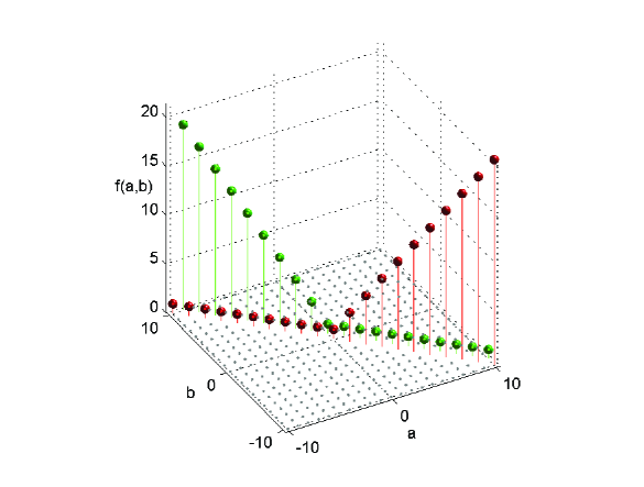
Figure 1. fp-$S$-theory for ${\mathbb{P}}^{1}$, where $f(a,b)=\operatorname{fpd}(\Sigma^{a}\circ S^{b})$.

5.2. Frobenius-Perron theory of the quiver $A_{2}$

We start with the following example.

Example 5.2.

Let $A$ be the ${\mathbb{Z}}$-graded algebra $\Bbbk[x]/(x^{2})$ with $\deg x=1$. Let ${\mathcal{C}}:=\operatorname{gr}-A$ be the category of finitely generated graded left $A$-modules. Let $\sigma:=(-)$ be the degree shift functor of ${\mathcal{C}}$. It is clear that $\sigma$ is an autoequivalence of ${\mathcal{C}}$. Let ${\mathfrak{A}}$ be the additive subcategory of ${\mathcal{C}}$ generated by $\sigma^{n}(A)=A(n)$ for all $n\in{\mathbb{Z}}$. Note that ${\mathfrak{A}}$ is not abelian and that every object in ${\mathfrak{A}}$ is of the form $\bigoplus_{n\in{\mathbb{Z}}}A(n)^{\oplus p_{n}}$ for some integers $p_{n}\geq 0$. Since the Hom-set in the graded module category consists of homomorphisms of degree zero, we have

$$\operatorname{Hom}_{\mathfrak{A}}(A,A(n))=\begin{cases}\Bbbk&n=0,1\\ 0&{\rm{otherwise}}\end{cases}.$$

In the following diagram each arrow represents $1$-dimensional Hom for all possible $\operatorname{Hom}$-set for different objects $A(n)$

(E5.2.1) $$\cdots\longrightarrow A(-2)\longrightarrow A(-1)\longrightarrow A(0)\longrightarrow A(1)\longrightarrow A(2)\longrightarrow\cdots$$

(where the number of arrows from $A(m)$ to $A(n)$ agrees with $\dim\operatorname{Hom}(A(m),A(n))$). It is easy to see that the set of indecomposable objects is $\{A(n)\}_{n\in{\mathbb{Z}}}$, which is also the set of bricks in ${\mathfrak{A}}$.

Lemma 5.3.

Retain the notation as in Example 5.2. When restricting $\sigma$ onto the category ${\mathfrak{A}}$, we have, for every $m\geq 1$,

(E5.3.1) $$\operatorname{fpd}^{m}(\sigma^{n})=\begin{cases}1&n=0,1,\\ 0&{\rm{otherwise}}\end{cases}.$$

Proof.

When $n=0$, (E5.3.1) is trivial. Let $n=1$. For each set $\phi\in\Phi_{m,b}$, we can assume that $\phi=\{A(d_{1}),A(d_{2},),\cdots,A(d_{m})\}$ for a strictly increasing sequence $\{d_{i}\mid i=1,2,\cdots,m\}$. For any $i<j$, the $(i,j)$-entry of the adjacency matrix is

$$a_{ij}=\dim(A(d_{i}),A(d_{j}+1))=0.$$

Thus $A(\phi,\sigma)$ is a lower triangular matrix with

$$a_{ii}=\dim(A(d_{i}),A(d_{i}+1))=1.$$

Hence $\rho(A(\phi,\sigma))=1$. So $\operatorname{fpd}^{m}(\sigma)=1$.

Similarly, $\operatorname{fpd}^{m}(\sigma^{n})=0$ when $n>1$ as $\dim(A(d_{i}),A(d_{i}+2))=0$ for all $i$.

Let $n<0$. Let $\phi=\{A(d_{1}),A(d_{2},),\cdots,A(d_{m})\}\in\Phi_{m,b}$ where $d_{i}$ are strictly decreasing. Then $a_{ij}=\dim(A(d_{i}),A(d_{j}+n))=0$ for all $i\leq j$. Thus $\rho(A(\phi,\sigma^{n}))=0$ and (E5.3.1) follows in this case. ∎

Example 5.4.

Consider the quiver $A_{2}$

(E5.4.1) $$\bullet_{2}\longleftarrow\bullet_{1}.$$

Let $P_{i}$ (respectively, $I_{i}$) be the projective (respectively, injective) left $\Bbbk A_{2}$-modules corresponding to vertices $i$, for $i=1,2$, It is well-known that there are only three indecomposable left modules over $A_{2}$, with Auslander-Reiten quiver (or AR-quiver, for short)

(E5.4.2) $$P_{2}\longrightarrow P_{1}(=I_{2})\longrightarrow I_{1}$$

where each arrow represents a nonzero homomorphism (up to a scalar) [Sc1, Ex.1.13, pp.24-25]. The AR-translation (or translation, for short) $\tau$ is determined by $\tau(I_{1})=P_{2}$. Let ${\mathcal{T}}$ be $D^{b}(\operatorname{Mod}_{f.d.}-\Bbbk A_{2})$. The Auslander-Reiten theory can be extended from the module category to the derived category. It is direct that, in ${\mathcal{T}}$, we have the AR-quiver of all indecomposable objects

(E5.4.3)    

The above represents all possible nonzero morphisms (up to a scalar) between non-isomorphic indecomposable objects in ${\mathcal{T}}$. Note that ${\mathcal{T}}$ has a Serre functor $S$ and that the AR-translation $\tau$ can be extended to a functor of ${\mathcal{T}}$ such that $S=\Sigma\circ\tau$ [RVdB, Proposition I.2.3] or [Cr, Remarks (2), p. 23]. After we identifying

$$P_{2}[i]\leftrightarrow A(3i),\quad P_{1}[i]\leftrightarrow A(3i+1),\quad I_{1}[i]\leftrightarrow A(3i+2),$$

(E5.4.3) agrees with (E5.2.1). Using the above identification, at least when restricted to objects, we have

(E5.4.4) $$\Sigma(A(i)) \cong A(i+3),$$

(E5.4.5) $$\tau(A(i)) \cong A(i-2),$$

(E5.4.6) $$S(A(i)) \cong A(i+1).$$

It follows from the definition of the AR-quiver [ARS, VII] that the degree of $\tau$ is $-2$, see also [AS, Picture on p. 131]. Equation (E5.4.5) just means that the degree of $\tau$ is $-2$.

By equation (E5.4.6), the Serre functor $S$ satisfies the property of $\sigma$ defined in Example 5.2. By Lemma 5.3 or (E5.3.1), we have

$$\operatorname{fpd}^{n}(\Sigma^{a}\circ S^{b})=\operatorname{fpd}^{n}(\sigma^{3a+b})=\begin{cases}1&3a+b=0,1,\\ 0&{\rm{otherwise}}.\end{cases}$$

Therefore the fp-$S$-theory of ${\mathcal{T}}$ is given as above, and given as in Figure 2 (next page).

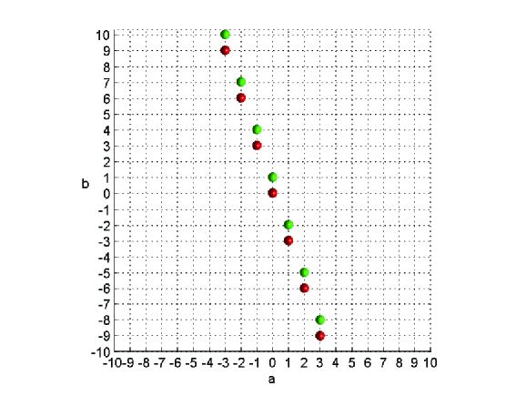
Figure 2. fp-$S$-theory for $A_{2}$

In particular, we have proven

$$\operatorname{fpgldim}(D^{b}(\operatorname{Mod}_{f.d.}-\Bbbk A_{2}))=\operatorname{fpd}(D^{b}(\operatorname{Mod}_{f.d.}-\Bbbk A_{2}))=\operatorname{fpd}(\Sigma)=0,$$

which is less than $\operatorname{gldim}\Bbbk A_{2}=1$.

5.3. An example of non-integral Frobenius-Perron dimension

In the next example, we “glue” $K_{2}$ in (E5.1.3) and $A_{2}$ in (E5.4.1) together.

Example 5.5.

Let $G_{2}$ be the quiver

(E5.5.1)

consisting of two vertices $1$ and $2$, with arrow $\alpha:2\to 1$ and $\beta,\gamma:1\to 2$ satisfying relations

(E5.5.2) $$R:\quad\beta\alpha=\gamma\alpha=0,\alpha\beta=\alpha\gamma=0.$$

Note that $(G_{2},R)$ is a quiver with relations. The corresponding quiver algebra with relations is a 5-dimensional algebra

$$A=\Bbbk e_{1}+\Bbbk e_{2}+\Bbbk\alpha+\Bbbk\beta+\Bbbk\gamma$$

satisfying, in addition to (E5.5.2),

(E5.5.3) $$e_{1}^{2}=e_{1},\quad e_{2}^{2}=e_{2},\quad 1=e_{1}+e_{2},$$

(E5.5.4) $$e_{2}\alpha=0,\quad\alpha e_{1}=0,\quad e_{1}\beta=e_{1}\gamma=0,\quad\beta e_{2}=\gamma e_{2}=0,$$

and

(E5.5.5) $$\alpha e_{2}=\alpha=e_{1}\alpha,\quad\beta e_{1}=\beta=e_{2}\beta,\quad\gamma e_{1}=\gamma=e_{2}\gamma.$$

We can use the following matrix form to represent the algebra $A$

$$A=\begin{pmatrix}\Bbbk e_{1}&\Bbbk\alpha\\ \Bbbk\beta+\Bbbk\gamma&\Bbbk e_{2}\end{pmatrix}.$$

For each $i=1,2$, let $S_{i}$ be the left simple $A$-module corresponding to the vertex $i$ and $P_{i}$ be the projective cover of $S_{i}$. Then $P_{1}\cong Ae_{1}$ is isomorphic to the first column of $A$, namely, $\begin{pmatrix}\Bbbk e_{1}\\ \Bbbk\beta+\Bbbk\gamma\end{pmatrix}$; and $P_{2}\cong Ae_{2}$ is isomorphic to the second column of $A$, namely, $\begin{pmatrix}\Bbbk\alpha\\ \Bbbk e_{2}\end{pmatrix}$.

We will show that the Frobenius-Perron dimension of the category of finite dimensional representations of $(G_{2},R)$ is $\sqrt{2}$, by using several lemmas below that contain some detailed computations.

Lemma 5.6.

Let $V=(V_{1},V_{2})$ be a representation of $(G_{2},R)$. Let $\overline{W}={\rm{im}}\;\alpha$ and $K=\ker\alpha$. Take a $\Bbbk$-space decomposition $V_{2}=W\oplus K$ where $W\cong\overline{W}$. Then there is a decomposition of $(G_{2},R)$-representations $V\cong(\overline{W}\oplus T,W\oplus K)\cong(\overline{W},W)\oplus(T,K)$ where $\alpha$ is the identity when restricted to $W$ (and identifying $W$ with $\overline{W}$) and is zero when restricted to $K$, where $\beta$ and $\gamma$ are zero when restricted to $\overline{W}$.

Proof.

Since $\overline{W}={\rm{im}}\;\alpha$, $V_{2}\cong W\oplus K$ where $K=\ker\alpha$ and $W\cong\overline{W}$. Write $V_{1}=\overline{W}\oplus T$ for some $\Bbbk$-subspace $T\subseteq V_{1}$. The assertion follows by using the relations in (E5.5.2). ∎

Recall that $A_{2}$ is the quiver given in (E5.4.1) and $K_{2}$ is the Kronecker quiver given in (E5.1.3). By the above lemma, the subrepresentation $(W,W)$ (where we identify $\overline{W}$ with $W$) is in fact a representation of $\begin{pmatrix}\Bbbk e_{1}&\Bbbk\alpha\\ 0&\Bbbk e_{2}\end{pmatrix}(\cong\Bbbk A_{2})$ and the subrepresentation $(T,K)$ is a representation of $\begin{pmatrix}\Bbbk e_{1}&0\\ \Bbbk\beta+\Bbbk\gamma&\Bbbk e_{2}\end{pmatrix}(\cong\Bbbk K_{2})$.

Let $I_{n}$ be the $n\times n$-identity matrix. Let $Bl(\lambda)$ denote the block matrix

$$\begin{pmatrix}\lambda&1&0&\cdots&0&0\\ 0&\lambda&1&\cdots&0&0\\ \ldots&\ldots&\ldots&\ldots&\ldots&\ldots\\ 0&0&0&\cdots&\lambda&1\\ 0&0&0&\cdots&0&\lambda\end{pmatrix}.$$

Lemma 5.7.

Suppose $\Bbbk$ is of characteristic zero. The following is a complete list of indecomposable representations of $(G_{2},R)$.

1. $P_{2}\cong(\Bbbk,\Bbbk)$, where $\alpha=I_{1}$ and $\beta=\gamma=0$.

2. $X_{n}(\lambda)=(K,K)$ with $\dim K=n$, where $\alpha=0$, $\beta=I_{n}$ and $\gamma=Bl(\lambda)$ for some $\lambda\in\Bbbk$.

3. $Y_{n}=(K,K)$ with $\dim K=n$, where $\alpha=0$, $\beta=Bl(0)$ and $\gamma=I_{n}$.

4. $S_{2,n}=(T,K)$ with $\dim T=n$ and $\dim K=n+1$, where $\alpha=0$, $\beta=(I_{n},0)$ and $\gamma=(0,I_{n})$.

5. $S_{1,n}=(T,K)$ with $\dim T=n+1$ and $\dim K=n$, where $\alpha=0$, $\beta=(I_{n},0)^{\tau}$ and $\gamma=(0,I_{n})^{\tau}$.

As a consequence, $\Bbbk G_{2}/(R)$ is of tame representation type [Definition 7.1].

Proof.

(1) By Lemma 5.6, this is the only case that could happen when $\alpha\neq 0$. Now we assume $\alpha=0$.

(2,3,4,5) If $\alpha=0$, then we are working with representations of Kronecker quiver $K_{2}$ (E5.1.3). The classification follows from a classical result of Kronecker [Ben, Theorem 4.3.2].

By (1-5), for each integer $n$, there are only finitely many 1-parameter families of indecomposable representations of dimension $n$. Therefore $A$ is of tame representation type. ∎

The following is a consequence of Lemma 5.7 and a direct computation.

Lemma 5.8.

Retain the hypotheses of Lemma 5.7. The following is a complete list of brick representations of $(G_{2},R)$.

1. $P_{2}\cong(\Bbbk,\Bbbk)$, where $\alpha=I_{1}$ and $\beta=\gamma=0$.

2. $X_{1}(\lambda)=(\Bbbk,\Bbbk)$, where $\alpha=0$, $\beta=I_{1}$ and $\gamma=\lambda I_{1}$ for some $\lambda\in\Bbbk$.

3. $Y_{1}=(\Bbbk,\Bbbk)$, where $\alpha=0$, $\beta=0$ and $\gamma=I_{1}$.

4. $S_{2,n}$ for $n\geq 0$.

5. $S_{1,n}$ for $n\geq 0$.

The set $\Phi_{1,b}$ consists of the above objects.

Let $X_{1}(\infty)$ denote $Y_{1}$. We have the following short exact sequences of $(G_{2},R)$-representations

$$0\to S_{1}\to P_{2}\to S_{2}\to 0,$$

$$0\to S_{2}\to X_{1}(\lambda)\to S_{1}\to 0,$$

$$0\to S_{2}^{n+1}\to S_{2,n}\to S_{1}^{n}\to 0,$$

$$0\to S_{2}^{n}\to S_{1,n}\to S_{1}^{n+1}\to 0,$$

$$0\to S_{2}^{2}\to S_{2,n}\to S_{1,n-1}\to 0,$$

where $n\geq 1$ for the last exact sequence, and have the following nonzero homs, where $A=\Bbbk G_{2}/(R)$,

$$\operatorname{Hom}_{A}(X_{1}(\lambda),S_{1,n}) \neq 0,\;\;\forall\;n\geq 1$$

$$\operatorname{Hom}_{A}(S_{2,n},X_{1}(\lambda)) \neq 0,\;\;\forall\;n\geq 1$$

$$\operatorname{Hom}_{A}(S_{2,m},S_{2,n}) \neq 0,\;\;\forall\;m\leq n$$

$$\operatorname{Hom}_{A}(S_{1,n},S_{1,m}) \neq 0,\;\;\forall\;m\leq n$$

$$\operatorname{Hom}_{A}(S_{2,n},S_{1,m}) \neq 0,\;\;\forall\;m+n\geq 1$$

Lemma 5.9.

Retain the hypotheses of Lemma 5.7. The following is the complete list of zero hom-sets between brick representations of $G_{2}$ in both directions.

1. $\operatorname{Hom}_{A}(X_{1}(\lambda),X_{1}(\lambda^{\prime}))=\operatorname{Hom}_{A}(X_{1}(\lambda^{\prime}),X_{1}(\lambda))=0$ if $\lambda\neq\lambda^{\prime}$ in $\Bbbk\cup\{\infty\}$.

2. $\operatorname{Hom}_{A}(S_{1},S_{2})=\operatorname{Hom}_{A}(S_{2},S_{1})=0$.

As a consequence, if $\phi\in\Phi_{n,b}$ for some $n\geq 2$, then $\phi=\{S_{1},S_{2}\}$ or $\phi=\{X_{1}(\lambda_{i})\}_{i=1}^{n}$ for different parameters $\{\lambda_{1},\cdots,\lambda_{n}\}$.

We also need to compute the $\operatorname{Ext}^{1}_{A}$-groups.

Lemma 5.10.

Retain the hypotheses of Lemma 5.7. Let $\lambda\neq\lambda^{\prime}$ be in $\Bbbk\cup\{\infty\}$.

1. $\operatorname{Ext}^{1}_{A}(X_{1}(\lambda),X_{1}(\lambda))=\operatorname{Hom}_{A}(X_{1}(\lambda),X_{1}(\lambda))=\Bbbk$.

2. $\operatorname{Ext}^{1}_{A}(X_{1}(\lambda),X_{1}(\lambda^{\prime}))=\operatorname{Hom}_{A}(X_{1}(\lambda),X_{1}(\lambda^{\prime}))=0$.

3. $\begin{pmatrix}\operatorname{Ext}^{1}_{A}(S_{1},S_{1})&\operatorname{Ext}^{1}_{A}(S_{1},S_{2})\\ \operatorname{Ext}^{1}_{A}(S_{2},S_{1})&\operatorname{Ext}^{1}_{A}(S_{2},S_{2})\end{pmatrix}=\begin{pmatrix}0&\Bbbk^{\oplus 2}\\ \Bbbk&0\end{pmatrix}.$

4. $\operatorname{Ext}^{1}_{A}(P_{2},P_{2})=0$.

5. $\dim\operatorname{Ext}^{1}_{A}(S_{2,n},S_{2,n})\leq 1$ for all $n$.

6. $\dim\operatorname{Ext}^{1}_{A}(S_{1,n},S_{1,n})\leq 1$ for all $n$.

Remark 5.11.

In fact, one can show the following stronger version of Lemma 5.10(5,6).

1. $\operatorname{Ext}^{1}_{A}(S_{2,n},S_{2,n})=0$ for all $n$.

2. $\operatorname{Ext}^{1}_{A}(S_{1,n},S_{1,n})=0$ for all $n$.

Proof of Lemma 5.10.

(1,2) Consider a minimal projective resolution of $X_{1}(\lambda)$

$$P_{1}\to P_{2}\xrightarrow{f_{\lambda}}P_{1}\to X_{1}(\lambda)\to 0$$

where $f_{\lambda}$ sends $e_{2}\in P_{2}$ to $\gamma-\lambda\beta\in P_{1}$. More precisely, we have

$$\begin{pmatrix}\Bbbk e_{1}\\ \Bbbk\beta+\Bbbk\gamma\end{pmatrix}\xrightarrow{e_{1}\to\alpha}\begin{pmatrix}\Bbbk\alpha\\ \Bbbk e_{2}\end{pmatrix}\xrightarrow{e_{2}\to\gamma-\lambda\beta}\begin{pmatrix}\Bbbk e_{1}\\ \Bbbk\beta+\Bbbk\gamma\end{pmatrix}\longrightarrow P_{1}/(\Bbbk(\gamma-\lambda\beta))\longrightarrow 0.$$

Applying $\operatorname{Hom}_{A}(-,X_{1}(\lambda^{\prime}))$ to the truncated projective resolution of the above, we obtain the following complex

$$\Bbbk\xleftarrow{\quad 0\quad}\Bbbk\xleftarrow{\quad g\quad}\Bbbk\longleftarrow 0.$$

If $g$ is zero, this is case (1). If $g\neq 0$, this is case (2).

(3) The proof is similar to the above by considering minimal projective resolutions of $S_{1}$ and $S_{2}$.

(4) This is clear since $P_{2}$ is a projective module.

(5,6) Let $S$ be either $S_{2,n}$ or $S_{1,n}$. By Example 5.1, $\operatorname{fpd}(\operatorname{Mod}_{f.d}-\Bbbk K_{2})=1$. This implies that

$$\dim\operatorname{Ext}^{1}_{\Bbbk K_{2}}(S,S)\leq 1$$

where $S$ is considered as an indecomposable $K_{2}$-module.

Let us make a comment before we continue the proof. Following a more careful analysis, one can actually show that

$$\operatorname{Ext}^{1}_{\Bbbk K_{2}}(S,S)=0.$$

Using this fact, the rest of the proof would show the assertions (5’,6’) in Remark 5.11.

Now we continue the proof. There is a projective cover $P_{1}^{b}\xrightarrow{f}S$ so that $\ker f$ is a direct sum of finitely many copies of $S_{2}$. Since $P_{2}$ is the projective cover of $S_{2}$, we have a minimal projective resolution

$$\longrightarrow P_{2}^{a}\longrightarrow P_{1}^{b}\longrightarrow S\longrightarrow 0$$

for some $a,b$. In the category $\operatorname{Mod}_{f.d}-\Bbbk K_{2}$, we have a minimal projective resolution of $S$

$$0\longrightarrow S_{2}^{a}\longrightarrow P_{1}^{b}\longrightarrow S\longrightarrow 0$$

where $S_{2}$ is a projective $\Bbbk K_{2}$-module. Hence we have a morphism of complexes

$$\begin{CD}@>{}>{}>P_{2}^{a}@>{}>{}>P_{1}^{b}@>{}>{}>S@>{}>{}>0\\ @V{}V{}V@ VV=V@V{}V{=}V\\ 0@>{}>{}>S_{2}^{a}@>{}>{}>P_{1}^{b}@>{}>{}>S@>{}>{}>0\end{CD}$$

Applying $\operatorname{Hom}_{A}(-,S)$ to above, we obtain that

$$\begin{CD}\cdots @<{}<{}<\operatorname{Hom}_{A}(P_{2}^{a},S)@<{h}<{}<\operatorname{Hom}_{A}(P_{1}^{b},S)@<{}<{}<\operatorname{Hom}_{A}(S,S)@<{}<{}<0\\ @A{g}A{}A@ AA=A@A{}A{=}A\\ \cdots @<{}<{}<\operatorname{Hom}_{A}(S_{2}^{a},S)@<{f}<{}<\operatorname{Hom}_{A}(P_{1}^{b},S)@<{}<{}<\operatorname{Hom}_{A}(S,S)@<{}<{}<0\\ \end{CD}$$

Note that $g$ is an isomorphism. Since $\dim\operatorname{Ext}^{1}_{\Bbbk K_{2}}(S,S)\leq 1$, the cokernel of $f$ has dimension at most 1. Since $g$ is an isomorphism, the cokernel of $h$ has dimension at most 1. This implies that $\operatorname{Ext}^{1}_{A}(S,S)$ has dimension at most 1. ∎

Proposition 5.12.

Let ${\mathfrak{A}}$ be the category $\operatorname{Mod}_{f.d.}-A$ where $A$ is in Example 5.5.

1. $\operatorname{fpd}^{n}{\mathfrak{A}}=\begin{cases}\sqrt{2}&n=2,\\ 1&n\neq 2.\end{cases}$ As a consequence, $\operatorname{fpd}{\mathfrak{A}}=\sqrt{2}$.

2. $SI({\mathfrak{A}})=2$.

3. $\operatorname{fpd}{\mathcal{A}}\geq\sqrt{2}$.

Proof.

(1) This is a consequence of Lemmas 5.9 and 5.10. Parts (2,3) follow from part (1). ∎

Remark 5.13.

Let $A$ be the algebra given in Example 5.5. We list some facts, comments and questions.

1. The algebra $A$ is non-connected ${\mathbb{N}}$-graded Koszul.

2. The minimal projective resolutions of $S_{1}$ and $S_{2}$ are

   $$\cdots\longrightarrow P_{1}^{\oplus 4}\longrightarrow P_{2}^{\oplus 4}\longrightarrow P_{1}^{\oplus 2}\longrightarrow P_{2}^{\oplus 2}\longrightarrow P_{1}\longrightarrow S_{1}\longrightarrow 0,$$

   and

   $$\cdots\longrightarrow P_{2}^{\oplus 4}\longrightarrow P_{1}^{\oplus 2}\longrightarrow P_{2}^{\oplus 2}\longrightarrow P_{1}\longrightarrow P_{2}\longrightarrow S_{2}\longrightarrow 0.$$

3. For $i\geq 0$, we have

   $$\operatorname{Ext}^{i}_{A}(S_{1},S_{1}) =\begin{cases}\Bbbk^{\oplus 2^{i/2}}&i\;{\text{is}}\;{\text{even}}\\ 0&\;{\text{is}}\;{\text{odd}}\end{cases}$$

   $$\operatorname{Ext}^{i}_{A}(S_{1},S_{2}) =\begin{cases}0&i\;{\text{is}}\;{\text{even}}\\ \Bbbk^{\oplus 2^{(i+1)/2}}&\;{\text{is}}\;{\text{odd}}\end{cases}$$

   $$\operatorname{Ext}^{i}_{A}(S_{2},S_{2}) =\begin{cases}\Bbbk^{\oplus 2^{i/2}}&i\;{\text{is}}\;{\text{even}}\\ 0&\;{\text{is}}\;{\text{odd}}\end{cases}$$

   $$\operatorname{Ext}^{i}_{A}(S_{2},S_{1}) =\begin{cases}0&i\;{\text{is}}\;{\text{even}}\\ \Bbbk^{\oplus 2^{(i-1)/2}}&\;{\text{is}}\;{\text{odd.}}\end{cases}$$

4. One can check that every algebra of dimension 4 or less has either infinite or integral $\operatorname{fpd}$. Hence, $A$ is an algebra of smallest $\Bbbk$-dimension that has finite non-integral (or irrational) $\operatorname{fpd}$. It is unknown if there is a finite dimensional algebra $A$ such that $\operatorname{fpd}(\operatorname{Mod}_{f.d.}-A)$ is transcendental.

5. Several authors have studied the connection between tame-wildness and complexity [BS, ES, Fa, FW, Kul, Ri]. The algebra $A$ is probably the first explicit example of a tame algebra with infinite complexity.

6. It follows from part (3) that the fp-curvature of ${\mathcal{A}}:=D^{b}(\operatorname{Mod}_{f.d.}-A)$ is $\sqrt{2}$ (some details are omitted). As a consequence, $\operatorname{fpg}({\mathcal{A}})=\infty$. By Theorem 8.3, the complexity of $A$ is $\infty$. We don’t know what $\operatorname{fpd}{\mathcal{A}}$ is.

6. $\sigma$-decompositions

We fix a category ${\mathcal{C}}$ and an endofunctor $\sigma$. For a set of bricks $B$ in ${\mathcal{C}}$ (or a set of atomic objects when ${\mathcal{C}}$ is triangulated), we define

$$\operatorname{fpd}^{n}\mid_{B}(\sigma)=\sup\{\rho(A(\phi,\sigma))\;\mid\;\phi:=\{X_{1},\cdots,X_{n}\}\in\Phi_{n,b},\;\;{\rm{and}}\;\;X_{i}\in B\;\;\forall i\}.$$

Let $\Lambda:=\{\lambda\}$ be a totally ordered set. We say a set of bricks $B$ in ${\mathcal{C}}$ has a $\sigma$-decomposition $\{B^{\lambda}\}_{\lambda\in\Lambda}$ (based on $\Lambda$) if the following holds.

1. $B$ is a disjoint union $\bigcup_{\lambda\in\Lambda}B^{\lambda}$.

2. If $X\in B^{\lambda}$ and $Y\in B^{\delta}$ with $\lambda<\delta$, $\operatorname{Hom}_{\mathcal{C}}(X,\sigma(Y))=0$.

The following lemma is easy.

Lemma 6.1.

Let $n$ be a positive integer. Suppose that $B$ has a $\sigma$-decomposition $\{B^{\lambda}\}_{\lambda\in\Lambda}$. Then

$$\operatorname{fpd}^{n}|_{B}(\sigma)\leq\sup_{\lambda\in\Lambda,m\leq n}\{\operatorname{fpd}^{m}|_{B^{\lambda}}(\sigma)\}.$$

Proof.

Let $\phi$ be a brick set that is used in the computation of $\operatorname{fpd}^{n}|_{B}(\sigma)$. Write

(E6.1.1) $$\phi=\phi_{\lambda_{1}}\cup\cdots\cup\phi_{\lambda_{s}}$$

where $\lambda_{i}$ is strictly increasing and $\phi_{\lambda_{i}}=\phi\cap B^{\lambda_{i}}$. For any objects $X\in\phi^{\lambda_{i}}$ and $Y\in\phi^{\lambda_{j}}$, where $\lambda_{i}<\lambda_{j}$, by definition, $\operatorname{Hom}_{\mathcal{C}}(X,\sigma(Y))=0$. Listing the objects in $\phi$ in the order that suggested by (E6.1.1), then the adjacency matrix of $(\phi,\sigma)$ is of the form

$$A(\phi,\sigma)=\begin{pmatrix}A_{11}&0&0&\cdots&0\\ \ast&A_{22}&0&\cdots&0\\ \ast&\ast&A_{33}&\cdots&0\\ \ldots&\ldots&\ldots&\ldots&0\\ \ast&\ast&\ast&\cdots&A_{ss}\end{pmatrix}$$

where each $A_{ii}$ is the adjacency matrix $A(\phi_{\lambda_{i}},\sigma)$. By definition,

$$\rho(A_{ii})\leq\operatorname{fpd}^{s_{i}}\mid_{B^{\lambda_{i}}}(\sigma)$$

where $s_{i}$ is the size of $A_{ii}$, which is no more than $n$. Therefore

$$\rho(A(\phi,\sigma))=\max_{i}\{\rho(A_{ii})\}\leq\sup_{\lambda\in\Lambda,m\leq n}\{\operatorname{fpd}^{m}|_{B^{\lambda}}(\sigma)\}.$$

The assertion follows. ∎

We give some examples of $\sigma$-decompositions.

Example 6.2.

Let ${\mathfrak{A}}$ be an abelian category and ${\mathcal{A}}$ be the derived category $D^{b}({\mathfrak{A}})$. Let $[n]$ be the $n$-fold suspension $\Sigma^{n}$.

1. Suppose that $\alpha$ is an endofunctor of ${\mathfrak{A}}$ and $\overline{\alpha}$ is the induced endofunctor of ${\mathcal{A}}$. For each $n\in{\mathbb{Z}}$, let $B^{n}:=\{M[-n]\mid M\;\;{\rm{is}}\;{\rm{a}}\;{\rm{brick}}\;{\rm{in}}\;{\mathfrak{A}}\}$ and $B:=\bigcup_{n\in{\mathbb{Z}}}B^{n}$. If $M_{i}[-n_{i}]\in B^{n_{i}}$, for $i=1,2$, such that $n_{1}<n_{2}$, then

   $$\operatorname{Hom}_{\mathcal{A}}(M_{1}[-n_{1}],\overline{\alpha}(M_{2}[-n_{2}]))=\operatorname{Ext}_{\mathfrak{A}}^{n_{1}-n_{2}}(M_{1},\alpha(M_{2}))=0.$$

   Then $B$ has a $\overline{\alpha}$-decomposition $\{B^{n}\}_{n\in{\mathbb{Z}}}$ based on ${\mathbb{Z}}$.

2. Suppose $g:=\operatorname{gldim}{\mathfrak{A}}<\infty$. Let $\sigma$ be the functor $\Sigma^{g}\circ\overline{\alpha}$. For each $n\in{\mathbb{Z}}$, let $B^{n}:=\{M[n]\mid M\;\;{\rm{is}}\;{\rm{a}}\;{\rm{brick}}\;{\rm{in}}\;{\mathfrak{A}}\}$ and $B:=\bigcup_{n\in{\mathbb{Z}}}B^{n}$. If $M_{i}[n_{i}]\in B^{n_{i}}$, for $i=1,2$, such that $n_{1}<n_{2}$, then

   $$\operatorname{Hom}_{\mathcal{A}}(M_{1}[n_{1}],\sigma(M_{2}[n_{2}]))=\operatorname{Ext}_{\mathfrak{A}}^{n_{2}-n_{1}+g}(M_{1},\alpha(M_{2}))=0.$$

   Then $B$ has a $\sigma$-decomposition $\{B^{n}\}_{n\in{\mathbb{Z}}}$ based on ${\mathbb{Z}}$.

Example 6.3.

Let $C$ be a smooth projective curve and let ${\mathfrak{A}}$ be the the category of coherent sheaves over $C$. Every coherent sheaf over $C$ is a direct sum of a torsion subsheaf and a locally free subsheaf. Define

$$B^{0} =\{T\;\;{\rm{is}}\;\;{\rm{a}}\;\;{\rm{torsion}}\;\;{\rm{brick}}\;\;{\rm{object}}\;\;{\rm{in}}\;\;{\mathfrak{A}}\},$$

$$B^{-1} =\{F\;\;{\rm{is}}\;\;{\rm{a}}\;\;{\rm{locally}}\;{\rm{free}}\;\;{\rm{brick}}\;\;{\rm{object}}\;\;{\rm{in}}\;\;{\mathfrak{A}}\}$$

and

$$B=B^{-1}\cup B^{0}.$$

Let $\sigma$ be the functor $E^{1}:=\operatorname{Ext}^{1}_{\mathfrak{A}}(-,-)$. If $F\in B^{-1}$ and $T\in B^{0}$, then

$$\operatorname{Ext}^{1}_{\mathfrak{A}}(F,T)=0.$$

Hence, $B$ has an $E^{1}$-decomposition based on the totally ordered set $\Lambda:=\{-1,0\}$.

The next example is given in [BB].

Example 6.4.

Let $C$ be an elliptic curve. Let ${\mathfrak{A}}$ be the the category of coherent sheaves over $C$ and ${\mathcal{A}}$ be the derived category $D^{b}({\mathfrak{A}})$.

First we consider coherent sheaves. Let $\Lambda$ be the totally ordered set ${\mathbb{Q}}\cup\{+\infty\}$. The slope of a coherent sheaf $X\neq 0$ [BB, Definition 4.6] is defined to be

$$\mu(X):=\frac{\chi(X)}{\operatorname{rk}(X)}\in\Lambda$$

where $\chi(X)$ is the Euler characteristic of $X$ and $\operatorname{rk}(X)$ is the rank of $X$. If $X$ and $Y$ are bricks such that $\mu(X)<\mu(Y)$, by [BB, Corollary 4.11], $X$ and $Y$ are semistable, and thus by [BB, Proposition 4.9(1)], $\operatorname{Hom}_{\mathfrak{A}}(Y,X)=0$. By Serre duality (namely, Calabi-Yau property),

(E6.4.1) $$\operatorname{Hom}_{\mathcal{A}}(X,Y[1])=\operatorname{Ext}^{1}_{\mathfrak{A}}(X,Y)=\operatorname{Hom}_{\mathfrak{A}}(Y,X)^{*}=0.$$

Write $B=\Phi_{1,b}({\mathfrak{A}})$ and $B^{\lambda}$ be the set of (semistable) bricks with slope $\lambda$. Then $B=\bigcup_{\lambda\in\Lambda}B^{\lambda}$. By (E6.4.1), $\operatorname{Ext}^{1}_{\mathfrak{A}}(X,Y)=0$ when $X\in B^{\lambda}$ and $Y\in B^{\nu}$ with $\lambda<\nu$. Hence $B$ has an $E^{1}$-decomposition. By Lemma 6.1, for every $n\geq 1$,

$$\operatorname{fpd}^{n}(E^{1})=\operatorname{fpd}^{n}|_{B}(E^{1})\leq\sup_{\lambda\in\Lambda,m\leq n}\{\operatorname{fpd}^{m}|_{B^{\lambda}}(E^{1})\}.$$

Next we compute $\operatorname{fpd}^{n}|_{B^{\lambda}}(E^{1})$. Let $SS^{\lambda}$ be the full subcategory of ${\mathfrak{A}}$ consisting of semistable coherent sheaves of slope $\lambda$. By [BB, Summary], $SS^{\lambda}$ is an abelian category that is equivalent to $SS^{\infty}$. Therefore one only needs to compute $\operatorname{fpd}^{n}|_{B^{\infty}}(E^{1})$ in the category $SS^{\infty}$. Note that $SS^{\infty}$ is the abelian category of torsion sheaves and every brick object in $SS^{\infty}$ is of the form ${\mathcal{O}}_{p}$ for some $p\in C$. In this case, $A(\phi,E^{1})$ is the identity matrix. Consequently, $\rho(A(\phi,E^{1}))=1$. This shows that $\operatorname{fpd}^{n}|_{B^{\lambda}}(E^{1})=\operatorname{fpd}^{n}|_{B^{\infty}}(E^{1})=1$ for all $n\geq 1$. It is clear that $\operatorname{fpd}^{n}(E^{1})\geq\operatorname{fpd}^{n}|_{B^{\infty}}(E^{1})=1$. Combining with Lemma 6.1, we obtain that $\operatorname{fpd}^{n}(E^{1})=1$ for all $n$. (The above approach works for functors other than $E^{1}$.)

Finally we consider the fp-dimension for the derived category ${\mathcal{A}}$. It follows from Theorem 3.5(3) that

$$\operatorname{fpd}^{n}(\Sigma)=\operatorname{fpd}^{n}(E^{1})=1$$

for all $n\geq 1$. By definition,

$$\operatorname{fpd}({\mathcal{A}})=\operatorname{fpd}({\mathfrak{A}})=1.$$

As we explained before $\operatorname{fpd}$ is an indicator of the representation types of categories.

Drozd-Greuel studied a tame-wild dichotomy for vector bundles on projective curves [DrG] and introduced the notion of VB-finite, VB-tame and VB-wild similar to the corresponding notion in the representation theory of finite dimensional algebras. In [DrG] Drozd-Greuel showed the following:

Let $C$ be a connected smooth projective curve. Then

1. $C$ is VB-finite if and only if $C$ is ${\mathbb{P}}^{1}$.

2. $C$ is VB-tame if and only if $C$ is elliptic (that is, of genus 1).

3. $C$ is VB-wild if and only if $C$ has genus $g\geq 2$.

We now prove a fp-version of Drozd-Greuel’s result [DrG, Theorem 1.6]. We thank Max Lieblich for providing ideas in the proof of Proposition 6.5(3) next.

Proposition 6.5.

Suppose $\Bbbk={\mathbb{C}}$. Let ${\mathbb{X}}$ be a connected smooth projective curve and let $g$ be the genus of ${\mathbb{X}}$.

1. If $g=0$ or ${\mathbb{X}}={\mathbb{P}}^{1}$, then $\operatorname{fpd}\;D^{b}(coh(\mathbb{X}))=1.$

2. If $g=1$ or ${\mathbb{X}}$ is an elliptic curve, then $\operatorname{fpd}\;D^{b}(coh(\mathbb{X}))=1.$

3. If $g\geq 2$, then $\operatorname{fpd}\;D^{b}(coh(\mathbb{X}))=\infty$.

Proof.

(1) The assertion follows from (E5.1.4).

(2) The assertion follows from Example 6.4.

(3) By Theorem 3.5(4), $\operatorname{fpd}(D^{b}(coh({\mathbb{X}})))=\operatorname{fpd}(coh({\mathbb{X}}))$. Hence it suffices to show that $\operatorname{fpd}(coh({\mathbb{X}}))=\infty$.

For each $n$, let $\{x_{i}\}_{i=1}^{n}$ be a set of $n$ distinct points on ${\mathbb{X}}$. By [DrG, Lemma 1.7], we might further assume that $2x_{i}\not\sim x_{j}+x_{k}$ for all $i\neq j$, as divisors on ${\mathbb{X}}$. Write $\mathcal{E}_{i}:={\mathcal{O}}(x_{i})$ for all $i$. By [DrG, p.11], $\operatorname{Hom}_{{\mathcal{O}}_{\mathbb{X}}}(\mathcal{E}_{i},\mathcal{E}_{j})=0$ for all $i\neq j$, which is also a consequence of a more general result [HL, Proposition 1.2.7]. It is clear that $\operatorname{Hom}_{{\mathcal{O}}_{\mathbb{X}}}(\mathcal{E}_{i},\mathcal{E}_{i})=\Bbbk$ for all $i$. Let $\phi_{n}$ be the set $\{\mathcal{E}_{1},\ldots,\mathcal{E}_{n}\}$. Then it is a brick set of non-isomorphic vector bundles on ${\mathbb{X}}$ (which are stable with ${\text{rank}}(\mathcal{E}_{i})=\deg(\mathcal{E}_{i})=1$ for all $i$).

Define the sheaf $\mathcal{H}_{ij}=\mathcal{H}om(\mathcal{E}_{i},\mathcal{E}_{j})$ for all $i,j$. Then $\deg(\mathcal{H}_{ij})=0.$ By the Riemann-Roch Theorem, we have

$$0 =\deg(\mathcal{H}_{ij})$$

$$=\chi(\mathcal{H}_{ij})-{\text{rank}}(\mathcal{H}_{ij})\chi(\mathcal{O}_{\mathbb{X}})$$

$$=\dim\operatorname{Hom}_{\mathcal{O}_{\mathbb{X}}}(\mathcal{E}_{i},\mathcal{E}_{j})-\dim\operatorname{Ext}^{1}_{\mathcal{O}_{\mathbb{X}}}(\mathcal{E}_{i},\mathcal{E}_{j})-(1-g)$$

$$=\delta_{ij}-\dim\operatorname{Ext}^{1}_{\mathcal{O}_{\mathbb{X}}}(\mathcal{E}_{i},\mathcal{E}_{j})+(g-1),$$

which implies that $\dim\operatorname{Ext}^{1}_{\mathcal{O}_{\mathbb{X}}}(\mathcal{E}_{i},\mathcal{E}_{j})=g-1+\delta_{ij}$. This formula was also given in [DrG, p.11 before Lemma 1.7] when $i\neq j$.

Define the matrix $A_{n}$ with entries $a_{ij}:=\dim\operatorname{Ext}^{1}_{\mathcal{O}_{\mathbb{X}}}(\mathcal{E}_{i},\mathcal{E}_{j})=g-1+\delta_{ij}$, which is the adjacency matrix of $(\phi_{n},E^{1})$. This matrix has entries $g$ along the diagonal and entries $g-1$ everywhere else. Therefore the vector $(1,\ldots,1)$ is an eigenvector for this matrix with eigenvalue $n(g-1)+1$. So $\rho(A_{n})\geq n(g-1)+1\geq n+1$. Since we can define $\phi_{n}$ for arbitrarily large $n$, we must have $\operatorname{fpd}(coh({\mathbb{X}}))=\infty.$ ∎

Question 6.6.

Let ${\mathbb{X}}$ be a smooth irreducible projective curve of genus $g\geq 2$. Is $\operatorname{fpd}^{n}({\mathbb{X}})$ finite for each $n$? If yes, do these invariants recover $g$?

Proposition 6.7.

Suppose $\Bbbk={\mathbb{C}}$. Let ${\mathbb{Y}}$ be a smooth projective scheme of dimension at least 2. Then

$$\operatorname{fpd}^{1}(coh({\mathbb{Y}}))=\operatorname{fpd}(coh({\mathbb{Y}}))=\operatorname{fpd}^{1}(D^{b}(coh({\mathbb{Y}})))=\operatorname{fpd}(D^{b}(coh({\mathbb{Y}})))=\infty.$$

Proof.

It is clear that $\operatorname{fpd}^{1}(coh({\mathbb{Y}}))$ is smallest among these four invariants. It suffices to show that $\operatorname{fpd}^{1}(coh({\mathbb{Y}}))=\infty$.

It is well-known that ${\mathbb{Y}}$ contains an irreducible projective curve ${\mathbb{X}}$ of arbitrarily large (either geometric or arithmetic) genus, see, for example, [CFZ, Theorem 0.1] or [Ch, Theorems 1 and 2]. Let ${\mathcal{O}}_{\mathbb{X}}$ be the coherent sheaf corresponding to the curve ${\mathbb{X}}$ and let $g$ be the arithmetic genus of ${\mathbb{X}}$. In the abelian category $coh({\mathbb{X}})$, we have

$$\dim\operatorname{Ext}^{1}_{\mathcal{O}_{\mathbb{X}}}(\mathcal{O}_{\mathbb{X}},\mathcal{O}_{\mathbb{X}})=\dim H^{1}({\mathbb{X}},\mathcal{O}_{\mathbb{X}})=g.$$

Since $coh({\mathbb{X}})$ is a full subcategory of $coh({\mathbb{Y}})$, we have

$$\dim\operatorname{Ext}^{1}_{\mathcal{O}_{\mathbb{Y}}}(\mathcal{O}_{\mathbb{X}},\mathcal{O}_{\mathbb{X}})\geq\dim\operatorname{Ext}^{1}_{\mathcal{O}_{\mathbb{X}}}(\mathcal{O}_{\mathbb{X}},\mathcal{O}_{\mathbb{X}})=g.$$

By taking $\phi=\{\mathcal{O}_{\mathbb{X}}\}$, one sees that $\operatorname{fpd}^{1}(coh({\mathbb{Y}}))\geq\operatorname{fpd}^{1}(coh({\mathbb{X}}))\geq g$ for all such ${\mathbb{X}}$. Since $g$ can be arbitrarily large, the assertion follows. ∎

7. Representation types

7.1. Representation types

We first recall some known definitions and results.

Definition 7.1.

Let $A$ be a finite dimensional algebra.

1. We say $A$ is of finite representation type if there are only finitely many isomorphism classes of finite dimensional indecomposable left $A$-modules.

2. We say $A$ is tame or of tame representation type if it is not of finite representation type, and for every $n\in{\mathbb{N}}$, all but finitely many isomorphism classes of $n$-dimensional indecomposables occur in a finite number of one-parameter families.

3. We say $A$ is wild or of wild representation type if, for every finite dimensional $\Bbbk$-algebra $B$, the representation theory of $B$ can be embedded into that of $A$.

The following is the famous trichotomy result due to Drozd [Dr1].

Theorem 7.2 (Drozd’s trichotomy theorem).

Every finite dimensional algebra is either of finite, tame, or wild representation type.

Remark 7.3.

1. An equivalent and more precise definition of a wild algebra is the following. An algebra $A$ is called wild if there is a faithful exact embedding of abelian categories

   (E7.3.1) $$Emb:\quad\operatorname{Mod}_{f.d.}-\Bbbk\langle x,y\rangle\to\operatorname{Mod}_{f.d.}-A$$

   that respects indecomposability and isomorphism classes.

2. A stronger notion of wildness is the following. An algebra $A$ is called strictly wild, also called fully wild, if $Emb$ in (E7.3.1) is a fully faithful embedding.

3. It is clear that strictly wild is wild. The converse is not true.

We collect some celebrated results in terms of representation types of path algebras [Ga1] and [Na, DoF].

Theorem 7.4.

Let $Q$ be a finite connected quiver.

1. [Ga1] The path algebra $\Bbbk Q$ is of finite representation type if and only if the underlying graph of $Q$ is a Dynkin diagram of type $ADE$.

2. [Na, DoF] The path algebra $\Bbbk Q$ is of tame representation type if and only if the underlying graph of $Q$ is an extended Dynkin diagram of type $\widetilde{A}\widetilde{D}\widetilde{E}$.

Our main goal in this section is to prove Theorem 0.3. We thank Klaus Bongartz for suggesting the following lemma.

Lemma 7.5.

[B1] Let $A$ be a finite dimensional algebra that is strictly wild. Then, for each integer $a>0$, there is a finite dimensional brick left $A$-module $N$ such that $\dim\operatorname{Ext}^{1}_{A}(N,N)\geq a$.

Proof.

Let $V$ be the vector space $\bigoplus_{i=1}^{a}\Bbbk x_{i}$ and let $B$ be the finite dimensional algebra $\Bbbk\langle V\rangle/(V^{\otimes 2})$. By [B2, Theorem 2(i)], there is a fully faithful exact embedding

$$\operatorname{Mod}_{f.d.}-B\longrightarrow\operatorname{Mod}_{f.d.}-\Bbbk\langle x,y\rangle.$$

Since $A$ is strictly wild, there is a fully faithful exact embedding

$$\operatorname{Mod}_{f.d.}-\Bbbk\langle x,y\rangle\longrightarrow\operatorname{Mod}_{f.d.}-A.$$

Hence we have a fully faithful exact embedding

(E7.5.1) $$F:\quad\operatorname{Mod}_{f.d.}-B\longrightarrow\operatorname{Mod}_{f.d.}-A.$$

Let $S$ be the trivial $B$-module $B/B_{\geq 1}$. It follows from an easy calculation that $\dim\operatorname{Ext}^{1}_{B}(S,S)=\dim(V)^{*}=a$. Since $F$ is fully faithful exact, $F$ induces an injection

$$F:\operatorname{Ext}^{1}_{B}(S,S)\longrightarrow\operatorname{Ext}^{1}_{A}(F(S),F(S)).$$

Thus $\dim\operatorname{Ext}^{1}_{A}(F(S),F(S))\geq a$. Since $S$ is simple, it is a brick. Hence, $F(S)$ is a brick. The assertion follows by taking $N=F(S)$. ∎

Proposition 7.6.

1. Let $A$ be a finite dimensional algebra that is strictly wild, then

   $$\operatorname{fpd}^{1}(E^{1})=\operatorname{fpd}({\mathfrak{A}})=\operatorname{fpd}({\mathcal{A}})=\infty.$$

2. If $A:=\Bbbk Q$ is wild, then

   $$\operatorname{fpd}^{1}(E^{1})=\operatorname{fpd}({\mathfrak{A}})=\operatorname{fpd}({\mathcal{A}})=\infty.$$

Proof.

(1) For each integer $a$, by Lemma 7.5, there is a brick $N$ in ${\mathfrak{A}}$ such that $\operatorname{Ext}^{1}_{\mathfrak{A}}(N,N)\geq a$. Hence $\operatorname{fpd}^{1}(E^{1})\geq a$. Since $a$ is arbitrary, $\operatorname{fpd}^{1}(E^{1})=\infty$. Consequently, $\operatorname{fpd}({\mathfrak{A}})=\infty$. By Lemma 2.9, $\operatorname{fpd}({\mathcal{A}})=\infty$.

(2) It is well-known that a wild path algebra is strictly wild, see a comment of Gabriel [Ga2, p.149] or [Ar, Proposition 7]. The assertion follows from part (1). ∎

The following lemma is based on a well-understood AR-quiver theory for acyclic quivers of finite representation type and the hammock theory introduced by Brenner [Bre]. We refer to [RV] if the reader is interested in a more abstract version of the hammock theory.

For a class of quivers including all ADE quivers, there is a convenient (though not essential) way of positioning the vertices as in [AS, Example IV.2.6]. A quiver $Q$ is called well-positioned if the vertices of $Q$ are located so that all arrows are strictly from the right to the left of the same horizontal distance. For example, the following quiver $D_{n}$ is well-positioned:

Lemma 7.7.

Let $Q$ be a quiver such that

1. the underlying graph of $Q$ is a Dynkin diagram of type $A$, or $D$, or $E$, and that

2. $Q$ is well-positioned.

Let $A=\Bbbk Q$ and let $M,N$ be two indecomposable left $A$-modules in the AR-quiver of $A$. Then the following hold.

1. There is a standard way of defining the order or degree for indecomposable left $A$-modules $M$, denoted by $\deg M$, such that all arrows in the the AR-quiver have degree 1, or equivalently, all arrows are from the left to the right of the same horizontal distance. As in (E5.4.2), when $Q=A_{2}$, $\deg P_{2}=0$, $\deg P_{1}=1$ and $\deg I_{1}=2$.

2. If $\operatorname{Hom}_{A}(M,N)\neq 0$, then $\deg M\leq\deg N$.

3. The degree of the AR-translation $\tau$ is $-2$.

4. If $\operatorname{Ext}^{1}_{A}(M,N)\neq 0$, then $\deg M\geq\deg N+2$.

5. There is no oriented cycle in the $E^{1}$-quiver of ${\mathfrak{A}}:=\operatorname{Mod}_{f.d.}-\Bbbk Q$, denoted by $Q^{E^{1}}_{\mathfrak{A}}$, defined before Lemma 2.10.

6. $\operatorname{fpd}({\mathfrak{A}})=0$.

Proof.

(1) This is a well-known fact in AR-quiver theory. For each given quiver $Q$ as described in (i,ii), one can build the AR-quiver by using the Auslander-Reiten translation $\tau$ and the Knitting Algorithm, see [Sc1, Ch. 3]. Some explicit examples are given in [Ga3, Ch. 6] and [Sc1, Ch. 3].

(2) This follows from (1). Note that the precise dimension of $\operatorname{Hom}_{A}(M,N)$ can be computed by using hammock theory [Bre, RV]. Some examples are given in [Sc1, Ch. 3].

(3) This follows from the definition of the translation $\tau$ in the AR-quiver theory [ARS, VII]. See also, [Cr, Remarks (2), p. 23].

(4) By Serre duality, $\operatorname{Ext}^{1}_{R}(M,N)=\operatorname{Hom}_{A}(N,\tau M)^{\ast}$ [RVdB, Proposition I.2.3] or [Cr, Lemma 1, p. 22]. If $\operatorname{Ext}^{1}_{R}(M,N)\neq 0$, then, by Serre duality and part (2), $\deg N\leq\deg\tau M=\deg M-2$. Hence $\deg M\geq\deg N+2$.

(5) In this case, every indecomposable module is a brick. Hence the $E^{1}$-quiver $Q^{E^{1}}_{\mathfrak{A}}$ has the same vertices as the AR-quiver. By part (4), if there is an arrow from $M$ to $N$ in the quiver $Q^{E^{1}}_{\mathfrak{A}}$, then $\deg M\geq\deg N+2$. This means that all arrows in $Q_{\mathfrak{A}}^{E^{1}}$ are from the right to the left. Therefore there is no oriented cycle in $Q^{E^{1}}_{\mathfrak{A}}$.

(6) This follows from part (5), Theorem 1.8(1) and Lemma 2.10. ∎

Theorem 7.8.

Let $Q$ be a finite quiver whose underlying graph is a Dynkin diagram of type $ADE$ and let $A=\Bbbk Q$. Then $\operatorname{fpd}({\mathfrak{A}})=\operatorname{fpd}({\mathcal{A}})=\operatorname{fpgldim}({\mathcal{A}})=0$.

Proof.

Since the path algebra $A$ is hereditary, ${\mathfrak{A}}$ is a-hereditary of global dimension 1. By Theorem 3.5(3), $\operatorname{fpd}({\mathfrak{A}})=\operatorname{fpd}({\mathcal{A}})$. If $Q_{1}$ and $Q_{2}$ are two quivers whose underlying graphs are the same, then, by Bernstein-Gelfand-Ponomarev (BGP) reflection functors [BGP], $D^{b}(\operatorname{Mod}_{f.d.}-\Bbbk Q_{1})$ and $D^{b}(\operatorname{Mod}_{f.d.}-\Bbbk Q_{2})$ are triangulated equivalent. Hence we only need prove the statement for one representative. Now we can assume that $Q$ satisfies the hypotheses (i,ii) of Lemma 7.7. By Lemma 7.7(6), $\operatorname{fpd}({\mathfrak{A}})=0$. Therefore $\operatorname{fpd}({\mathcal{A}})=0$, or equivalently, $\operatorname{fpd}(\Sigma)=0$. By Theorem 3.5(1), $\operatorname{fpd}(\Sigma^{i})=0$ for all $i\neq 0,1$. Therefore $\operatorname{fpgldim}({\mathcal{A}})=0$. ∎

7.2. Weighted projective lines

To prove Theorem 0.3, it remains to show part (2) of the theorem. Our proof uses a result of [CG] about weighted projective lines, which we now review. Details can be found in [GL, Section 1].

For $t\geq 1$, let ${\bf p}:=(p_{0},p_{1},\cdots,p_{t})$ be a $(t+1)$-tuple of positive integers, called the weight sequence. Let ${\bf D}:=(\lambda_{0},\lambda_{1},\cdots,\lambda_{t})$ be a sequence of distinct points of the projective line ${\mathbb{P}}^{1}$ over $\Bbbk$. We normalize ${\bf D}$ so that $\lambda_{0}=\infty$, $\lambda_{1}=0$ and $\lambda_{2}=1$ (if $t\geq 2$). Let

$$S:=\Bbbk[X_{0},X_{1},\cdots,X_{t}]/(X_{i}^{p_{i}}-X_{1}^{p_{1}}+\lambda_{i}X_{0}^{p_{0}},i=2,\cdots,t).$$

The image of $X_{i}$ in $S$ is denoted by $x_{i}$ for all $i$. Let ${\mathbb{L}}$ be the abelian group of rank 1 generated by $\overrightarrow{x_{i}}$ for $i=0,1,\cdots,t$ and subject to the relations

$$p_{0}\overrightarrow{x_{0}}=\cdots=p_{i}\overrightarrow{x_{i}}=\cdots=p_{t}\overrightarrow{x_{t}}=:\overrightarrow{c}.$$

The algebra $S$ is ${\mathbb{L}}$-graded by setting $\deg x_{i}=\overrightarrow{x_{i}}$. The corresponding weighted projective line, denoted by ${\mathbb{X}}({\bf p},{\bf D})$ or simply ${\mathbb{X}}$, is a noncommutative space whose category of coherent sheaves is given by the quotient category

$$coh({\mathbb{X}}):=\frac{\operatorname{gr}^{\mathbb{L}}-S}{\operatorname{gr}_{f.d.}^{\mathbb{L}}-S}$$

where $\operatorname{gr}^{\mathbb{L}}-S$ is the category of noetherian ${\mathbb{L}}$-graded left $S$-modules and $\operatorname{gr}_{f.d.}^{\mathbb{L}}-S$ is the full subcategory of $\operatorname{gr}^{\mathbb{L}}-S$ consisting of finite dimensional modules.

The weighted projective lines are classified into the following three classes:

$${\mathbb{X}}\;\;{\rm{is}}\;\;\begin{cases}domestic\;\;&{\rm{if}}\;\;{\bf p}\;\;{\rm{is}}\;(p,q),(2,2,n),(2,3,3),(2,3,4),(2,3,5);\\ tubular\;\;&{\rm{if}}\;\;{\bf p}\;\;{\rm{is}}\;(2,3,6),(3,3,3),(2,4,4),(2,2,2,2);\\ wild\;\;&{\rm{otherwise}}.\end{cases}$$

Let ${\mathbb{X}}$ be a weighted projective curve. Let $Vect({\mathbb{X}})$ be the full subcategory of $coh({\mathbb{X}})$ consisting of all vector bundles. Similar to the elliptic curve case [Example 6.4], one can define the concepts of degree, rank and slope of a vector bundle on a weighted projective curve ${\mathbb{X}}$, see [LM, Section 2] for details. For each $\mu\in{\mathbb{Q}}\cup\{\infty\}$, let $Vect_{\mu}({\mathbb{X}})$ be the full subcategory of $Vect({\mathbb{X}})$ consisting of all vector bundles of slope $\mu$.

Lemma 7.9.

Let ${\mathbb{X}}={\mathbb{X}}({\bf p},{\bf D})$ be a weighted projective line.

1. $coh({\mathbb{X}})$ is noetherian and hereditary.

2. $$D^{b}(coh({\mathbb{X}}))\cong\begin{cases}D^{b}(\operatorname{Mod}_{f.d.}-\Bbbk\widetilde{A}_{p,q})&{\rm{if}}\;\;{\bf p}=(p,q),\\ D^{b}(\operatorname{Mod}_{f.d.}-\Bbbk\widetilde{D}_{n})&{\rm{if}}\;\;{\bf p}=(2,2,n),\\ D^{b}(\operatorname{Mod}_{f.d.}-\Bbbk\widetilde{E}_{6})&{\rm{if}}\;\;{\bf p}=(2,3,3),\\ D^{b}(\operatorname{Mod}_{f.d.}-\Bbbk\widetilde{E}_{7})&{\rm{if}}\;\;{\bf p}=(2,3,4),\\ D^{b}(\operatorname{Mod}_{f.d.}-\Bbbk\widetilde{E}_{8})&{\rm{if}}\;\;{\bf p}=(2,3,5).\end{cases}$$

3. Let $M$ be a generic simple object in $coh({\mathbb{X}})$. Then $\operatorname{Ext}^{1}_{\mathbb{X}}(M,M)=1$.

4. $\operatorname{fpd}^{1}(coh({\mathbb{X}}))\geq 1$.

5. If ${\mathbb{X}}$ is tubular or domestic, then $\operatorname{Ext}^{1}_{\mathbb{X}}(X,Y)=0$ for all $X\in Vect_{\mu^{\prime}}({\mathbb{X}})$ and $Y\in Vect_{\mu}({\mathbb{X}})$ with $\mu^{\prime}<\mu$.

6. If ${\mathbb{X}}$ is domestic, then $\operatorname{Ext}^{1}_{\mathbb{X}}(X,Y)=0$ for all $X\in Vect_{\mu^{\prime}}({\mathbb{X}})$ and $Y\in Vect_{\mu}({\mathbb{X}})$ with $\mu^{\prime}\leq\mu$. As a consequence, $\operatorname{fpd}(\Sigma\mid_{Vect_{\mu^{\prime}}({\mathbb{X}})})=0$ for all $\mu<\infty$.

7. Suppose ${\mathbb{X}}$ is tubular. Then every indecomposable vector bundle ${\mathbb{X}}$ is semi-stable.

8. Suppose ${\mathbb{X}}$ is tubular and let $\mu\in{\mathbb{Q}}$. Then each $Vect_{\mu}({\mathbb{X}})$ is a uniserial category. Accordingly indecomposables in $Vect_{\mu}({\mathbb{X}})$ decomposes into Auslander-Reiten components, which all are tubes of finite rank.

Proof.

(1) This is well-known.

(2) [GL, 5.4.1].

(3) Let $M$ be a generic simple object. Then $M$ is a brick and $\operatorname{Ext}^{1}(M,M)=1$.

(4) Follows from (3) by taking $\phi:=\{M\}$.

(5) This is [Sc2, Corollary 4.34(i)] since tubular is also called elliptic in [Sc2].

(6) This is [Sc2, Comments after Corollary 4.34] since domestic is also called parabolic in [Sc2]. The consequence is clear.

(7) [GL, Theorem 5.6(i)].

(8) [GL, Theorem 5.6(iii)]. ∎

We will use the following result which is proved in [CG].

Theorem 7.10.

[CG] Let ${\mathbb{X}}$ be a weighted projective line.

1. If ${\mathbb{X}}$ is domestic, then $\operatorname{fpd}\;D^{b}(coh({\mathbb{X}}))=1$.

2. If ${\mathbb{X}}$ is tubular, then $\operatorname{fpd}\;D^{b}(coh({\mathbb{X}}))=1$.

3. If ${\mathbb{X}}$ is wild, then $\operatorname{fpd}\;D^{b}(coh({\mathbb{X}}))\geq\dim\operatorname{Hom}_{\mathbb{X}}({\mathcal{O}}_{\mathbb{X}},{\mathcal{O}}_{\mathbb{X}}(\overrightarrow{\omega}))$ where $\overrightarrow{\omega}$ is the dualizing element [GL, Sec. 1.2].

There is a similar statement for smooth complex projective curves [Proposition 6.5]. The authors are interested in answering the following question.

Question 7.11.

Let ${\mathbb{X}}$ be a wild weighted projective line. What is the exact value of $\operatorname{fpd}^{n}\;D^{b}(coh({\mathbb{X}}))$?

7.3. Tubes

The following example is studied in [CG], which is dependent on direct linear algebra calculations.

Example 7.12.

[CG] Let $\xi$ be a primitive $n$th root of unity. Let $T_{n}$ be the algebra

$$T_{n}:=\frac{\Bbbk\langle g,x\rangle}{(g^{n}-1,xg-\xi gx)}.$$

This algebra can be expressed by using a group action. Let $G$ be the group

$$\{g\mid g^{n}=1\}\cong{\mathbb{Z}}/(n)$$

acting on the polynomial ring $\Bbbk[x]$ by $g\cdot x=\xi x$. Then $T_{n}$ is naturally isomorphic to the skew group ring $\Bbbk[x]\ast G$. Let $\overrightarrow{A_{n-1}}$ denote the cycle quiver with $n$ vertices, namely, the quiver with one oriented cycle connecting $n$ vertices. It is also known that $T_{n}$ is isomorphic to the path algebra of the quiver $\overrightarrow{A_{n-1}}$. Then $\operatorname{fpd}(\operatorname{Mod}_{f.d.}-T_{n})=1$ by [CG].

7.4. Proof of Theorem 0.3

Proof of Theorem 0.3.

Part (1) follows from Theorems 7.4(1) and 7.8. Part (3) follows from Proposition 7.6(2). It remains to deal with part (2).

(2) By Theorem 7.4(2), $Q$ must be of type either $\overrightarrow{A_{n-1}}$, or $\widetilde{A}_{p,q}$, or $\widetilde{D}_{n}$, or $\widetilde{E}_{6,7,8}$. If $Q$ is of type $\overrightarrow{A_{n-1}}$, the assertion follows from Example 7.12. If $Q$ is of type $\widetilde{A}_{p,q}$, $\widetilde{D}_{n}$, or $\widetilde{E}_{6,7,8}$, the assertion follows from Lemma 7.9(2) and Theorem 7.10(1). ∎

8. Complexity

The concept of complexity was first introduced by Alperin-Evens in the study of group cohomology in 1981 [AE]. Since then the study of complexity has been extended to finite dimensional algebras, Frobenius algebras, Hopf algebras and commutative algebras. First we recall the classical definition of the complexity for finite dimensional algebras and then give a definition of the complexity for triangulated categories. We give the following modified (but equivalent) version, which can be generalized.

Definition 8.1.

Let $A$ be a finite dimensional algebra and $T=A/J(A)$ where $J(A)$ is the Jacobson radical of $A$. Let $M$ be a finite dimensional left $A$-module.

1. The complexity of $M$ is defined to be

   $$cx(M):=\limsup_{n\to\infty}\log_{n}(\dim\operatorname{Ext}^{n}_{A}(M,T))+1.$$

2. The complexity of the algebra $A$ is defined to be

   $$cx(A):=cx(T).$$

In the original definition of complexity by Alperin-Evens [AE] and in most of other papers, the dimension of $n$-syzygies is used instead of the dimension of the $\operatorname{Ext}^{n}$-groups, but it is easy to see that the asymptotic behavior of these two series are the same, therefore these give rise to the same complexity. It is well-known that $cx(M)\leq cx(A)$ for all finite dimensional left $A$-modules $M$. Next we introduce the notion of a complexity for a triangulated category which is partially motivated by the work in [BHZ, Section 4].

Definition 8.2.

Let ${\mathcal{T}}$ be a pre-triangulated category. Let $d$ be a real number.

1. The left subcategory of complexity less than $d$ is defined to be

   $${}_{d}{\mathcal{T}}:=\left\{X\in{\mathcal{T}}\mid\lim_{n\to\infty}\frac{\dim\operatorname{Hom}_{\mathcal{T}}(X,\Sigma^{n}(Y))}{n^{d-1}}=0,\forall\;Y\in{\mathcal{T}}\right\}.$$

2. The right subcategory of complexity less than $d$ is defined to be

   $${\mathcal{T}}_{d}:=\left\{X\in{\mathcal{T}}\mid\lim_{n\to\infty}\frac{\dim\operatorname{Hom}_{\mathcal{T}}(Y,\Sigma^{n}(X))}{n^{d-1}}=0,\forall\;Y\in{\mathcal{T}}\right\}.$$

3. The complexity of ${\mathcal{T}}$ is defined to be

   $$cx({\mathcal{T}}):=\inf\left\{d\mid{{}_{d}{\mathcal{T}}}={\mathcal{T}}\right\}$$

4. The Frobenius-Perron complexity of ${\mathcal{T}}$ is defined to be

   $$\operatorname{fpcx}({\mathcal{T}}):=\operatorname{fpg}(\Sigma)+1.$$

Note that it is not hard to show that $cx({\mathcal{T}})=\inf\left\{d\mid{{\mathcal{T}}_{d}}={\mathcal{T}}\right\}.$

Theorem 8.3.

Let ${\mathcal{T}}$ be a pre-triangulated category. Then $\operatorname{fpcx}({\mathcal{T}})\leq cx({\mathcal{T}})$.

Proof.

Let $d$ be any number strictly larger than $cx({\mathcal{T}})$. We need to show that $\operatorname{fpcx}({\mathcal{T}})\leq d$.

Let $\phi\in\Phi_{m,a}$ be an atomic set and let $X:=\bigoplus_{X_{i}\in\phi}X_{i}$. Then, by definition,

$$\lim_{n\to\infty}\frac{\dim\operatorname{Hom}_{\mathcal{T}}(X,\Sigma^{n}(X))}{n^{d-1}}=0.$$

Then there is a constant $C$ such that $\dim\operatorname{Hom}_{\mathcal{T}}(X,\Sigma^{n}(X))<Cn^{d-1}$ for all $n>0$. Since each $X_{i}$ is a direct summand of $X$, we have

$$a_{ij}(n):=\dim\operatorname{Hom}_{\mathcal{T}}(X_{i},\Sigma^{n}(X_{j}))<Cn^{d-1}$$

for all $i,j$. This means that each entry $a_{ij}(n)$ in the adjacency matrix of $A(\phi,\Sigma^{n})$ is less than $Cn^{d-1}$. Therefore $\rho(A(\phi,\Sigma^{n}))<mCn^{d-1}$. By Definition 2.3(3), $\operatorname{fpg}(\Sigma)\leq d-1$. Thus $\operatorname{fpcx}({\mathcal{T}})\leq d$ as desired. ∎

We will prove that the equality $\operatorname{fpcx}({\mathcal{T}})=cx({\mathcal{T}})$ holds under some extra hypotheses. Let $A$ be a finite dimensional algebra with a complete list of simple left $A$-modules $\{S_{1},\cdots,S_{w}\}$. We use $n$ for any integer and $i,j$ for integers between 1 and $w$. Define, for $i\leq j$,

$$p_{ij}(n):=\min\{\dim\operatorname{Ext}^{n}_{A}(S_{i},S_{j}),\dim\operatorname{Ext}^{n}_{A}(S_{j},S_{i})\}$$

and

$$P_{n}:=\max\{p_{ij}(n)\mid i\leq j\}.$$

We say $A$ satisfies averaging growth condition (or AGC for short) if there are positive integers $C$ and $d$, independent of the choices of $n$ and $(i,j)$, such that

(E8.3.1) $$\dim\operatorname{Ext}^{n}_{A}(S_{i},S_{j})\leq C\max\{P_{n-d},P_{n-d+1},\cdots,P_{n+d}\}$$

for all $n$ and all $1\leq i,j\leq w$.

Theorem 8.4.

Let $A$ be a finite dimensional algebra and ${\mathcal{A}}=D^{b}(\operatorname{Mod}_{f.d.}-A)$.

1. $cx(A)=cx({\mathcal{A}})$. As a consequence, $cx(A)$ is a derived invariant.

2. If $A$ satisfies AGC, then $\operatorname{fpcx}({\mathcal{A}})=cx({\mathcal{A}})=cx(A)$. As a consequence, if $A$ is local or commutative, then $\operatorname{fpcx}({\mathcal{A}})=cx({\mathcal{A}})=cx(A)$.

We will prove Theorem 8.4 after the next lemma.

Let ${\mathcal{T}}$ be a pre-triangulated category with suspension $\Sigma$. We use $X,Y,Z$ for objects in ${\mathcal{T}}$. Fix a family $\phi$ of objects in ${\mathcal{T}}$ and a positive number $d$. Define

(E8.4.1) $${{}_{d}(\phi)} =\left\{X\in{\mathcal{T}}\mid\lim_{n\to\infty}\frac{\dim\operatorname{Hom}_{\mathcal{T}}(X,\Sigma^{n}(Y))}{n^{d-1}}=0,\forall\;Y\in\phi\right\},$$

(E8.4.2) $$(\phi)_{d} =\left\{X\in{\mathcal{T}}\mid\lim_{n\to\infty}\frac{\dim\operatorname{Hom}_{\mathcal{T}}(Y,\Sigma^{n}(X))}{n^{d-1}}=0,\forall\;Y\in\phi\right\},$$

(E8.4.3) $${{}^{d}(\phi)} =\left\{X\in{\mathcal{T}}\mid\lim_{n\to\infty}\frac{\sum_{i\leq n}\dim\operatorname{Hom}_{\mathcal{T}}(X,\Sigma^{i}(Y))}{n^{d}}=0,\forall\;Y\in\phi\right\},$$

(E8.4.4) $$(\phi)^{d} =\left\{X\in{\mathcal{T}}\mid\lim_{n\to\infty}\frac{\sum_{i\leq n}\dim\operatorname{Hom}_{\mathcal{T}}(Y,\Sigma^{i}(X))}{n^{d}}=0,\forall\;Y\in\phi\right\}.$$

Lemma 8.5.

The following are full thick pre-triangulated subcategories of ${\mathcal{T}}$ closed under direct summands.

1. ${{}_{d}(\phi)}$.

2. $(\phi)_{d}$.

3. ${{}^{d}(\phi)}$.

4. $(\phi)^{d}$.

Proof.

We only prove (1). The proofs of other parts are similar. Suppose $X\in{{}_{d}(\phi)}$. Using the fact $\lim_{n\to\infty}\frac{n^{d-1}}{(n+1)^{d-1}}=1$, we see that $X[1]=\Sigma(X)$ is in ${{}_{d}(\phi)}$. Similarly, $X[-1]$ is in ${{}_{d}(\phi)}$. If $f:X_{1}\to X_{2}$ be a morphism of objects in ${{}_{d}(\phi)}$, and let $X_{3}$ be the mapping cone of $f$, then, for each $Y\in\phi$, we have an exact sequence

$$\to\operatorname{Hom}_{\mathcal{T}}(X_{1},\Sigma^{n-1}(Y))\to\operatorname{Hom}_{\mathcal{T}}(X_{3},\Sigma^{n}(Y))\to\operatorname{Hom}_{\mathcal{T}}(X_{2},\Sigma^{n}(Y))\to$$

which implies that $X_{3}\in{{}_{d}(\phi)}$. Therefore ${{}_{d}(\phi)}$ is a thick pre-triangulated subcategory of ${\mathcal{T}}$. If $X\in{{}_{d}(\phi)}$ and $X=Y\oplus Z$, it is clear that $Y,Z\in{{}_{d}(\phi)}$. Therefore ${{}_{d}(\phi)}$ is closed under taking direct summands. ∎

Proof of Theorem 8.4.

(1) Let $c=cx(A)$. For every $d<c$, we have that

$$\limsup_{n\to\infty}\frac{\dim\operatorname{Ext}^{n}_{A}(T,T)}{n^{d-1}}=\infty$$

which implies that $T\not\in{{}_{d}{\mathcal{A}}}$. Therefore $d\leq cx({\mathcal{A}})$.

Conversely, let $d>c$. It follows from the definition that

$$\limsup_{n\to\infty}\frac{\dim\operatorname{Ext}^{n}_{A}(T,T)}{n^{d-1}}=0.$$

This means that $T\in(\{T\})_{d}$. Since $T$ generates ${\mathcal{A}}$, we have ${\mathcal{A}}=(\{T\})_{d}$. Again, since $T$ generates ${\mathcal{A}}$, we have ${\mathcal{A}}={\mathcal{A}}_{d}={{}_{d}{\mathcal{A}}}$. By definition, $d\geq cx({\mathcal{A}})$ as desired.

(2) Assume that $A$ satisfies AGC. Let

$$c_{1} =\operatorname{fpcx}({\mathcal{A}}),$$

$$c_{2} =\limsup_{n\to\infty}\log_{n}(C\max\{P_{n-d},P_{n-d+1},\cdots,P_{n+d}\})+1,$$

$$c_{3} =\limsup_{n\to\infty}\log_{n}(P_{n})+1,$$

$$c_{4} =cx(A)=cx({\mathcal{A}}).$$

By calculus, we have $c_{2}=c_{3}$. Let $\phi$ be the atomic set of simple objects $\{S_{i}\}_{i=1}^{w}$. Then $\rho(\phi,\Sigma^{n})\geq p_{ij}(n)$, for all $i,j$, by Lemma 1.7(2). So $\rho(\phi,\Sigma^{n})\geq P_{n}$. As a consequence, $c_{1}\geq c_{3}$. Let $T=A/J=\bigoplus_{i=1}^{w}S_{i}^{d_{i}}$ for some finite numbers $\{d_{i}\}_{i=1}^{w}$. Let $D$ be $\max_{i}\{d_{i}\}$. By AGC, namely, (E8.3.1),

$$\dim\operatorname{Ext}^{n}_{A}(T,T) =\sum_{i,j}d_{i}d_{j}\dim\operatorname{Ext}^{n}_{A}(S_{i},S_{j})$$

$$\leq w^{2}DC\max\{P_{n-d},P_{n-d+1},\cdots,P_{n+d}\}$$

which implies that $c_{4}=cx(A)=cx(T)\leq c_{2}$. Combining with Theorem 8.3, we have $c_{1}=c_{2}=c_{3}=c_{4}$ as desired.

If $A$ is local, then there is only one simple module $S_{1}$. Then (E8.3.1) is automatic. If $A$ is commutative, then $\operatorname{Ext}^{i}_{A}(S_{i},S_{j})=0$ for all $n$ and all $i\neq j$. Again, in this case, (E8.3.1) is obvious. The consequence follows from the main assertion. ∎

For all well-studied finite dimensional algebras $A$, (E8.3.1) holds. For example, the algebra $A$ in Example 5.5 satisfies AGC. This can be shown by using the computation given in Remark 5.13(3). It is natural to ask if every finite dimensional algebra satisfies AGC.

Lemma 8.6.

1. Let ${\mathfrak{A}}$ be an abelian category and ${\mathcal{A}}=D^{b}({\mathfrak{A}})$. If $\operatorname{gldim}{\mathfrak{A}}<\infty$, then $\operatorname{fpcx}({\mathcal{A}})=0$.

2. Let ${\mathcal{T}}$ be a pre-triangulated category. If $\operatorname{fpgldim}{\mathcal{T}}<\infty$, then $\operatorname{fpcx}({\mathcal{T}})=0$.

Proof.

Both are easy and proofs are omitted. ∎

We conclude with examples of non-integral $\operatorname{fpg}$ of a triangulated category.

Example 8.7.

(1) Let $\alpha$ be any real number in $\{0\}\cup\{1\}\cup[2,\infty)$. By [KL, Theorem 1.8, or p. 14], there is a finitely generated algebra $R$ with $\operatorname{GKdim}R=\alpha$. More precisely, [KL, Theorem 1.8] implies that there is a 2-dimensional vector space $V\subset R$ that generates $R$ such that, there are positive integers $a<b$, for every $n>0$,

$$an^{\alpha}<\dim(\Bbbk 1+V)^{n}<bn^{\alpha}.$$

Define a filtration ${\mathcal{F}}$ on $R$ by

$$F_{i}R=(\Bbbk 1+V)^{i},\quad\forall\;i.$$

Let $A$ be the associated graded algebra $\operatorname{gr}R$ with respect to this grading. Then $A$ is connected graded and generated by two elements in degree 1 and satisfying, for every $n>0$,

(E8.7.1) $$an^{\alpha}<\sum_{i=0}^{n}\dim A_{i}<bn^{\alpha}.$$

To match up with the definition of complexity, we further assume that there are $c<d$ such that, for every $n>0$,

(E8.7.2) $$cn^{\alpha-1}<\dim A_{n}<dn^{\alpha-1}.$$

This can be achieved, for example, by replacing $A$ by its polynomial extension $A[t]$ (with $\deg t=1$) and replacing $\alpha$ by $\alpha+1$.

Next we make $A$ a differential graded (dg) algebra by setting elements in $A_{i}$ to have cohomological degree $i$ and $d_{A}=0$. For this dg algebra, we denote the derived category of left dg $A$-modules by ${\mathcal{A}}$. Let ${\mathcal{O}}$ be the object ${}_{A}A$ in ${\mathcal{A}}$. By the definition of the cohomological degree of $A$, we have

(E8.7.3) $$\operatorname{Hom}_{\mathcal{A}}({\mathcal{O}},\Sigma^{i}{\mathcal{O}})=A_{i},\quad\forall\;i.$$

Let ${\mathcal{T}}$ be the full triangulated subcategory of ${\mathcal{A}}$ generated by ${\mathcal{O}}$. (E8.7.3) implies that ${\mathcal{O}}$ is an atomic object. Now using (E8.7.3) together with (E8.7.2), we obtain that

(E8.7.4) $$\operatorname{fpcx}({\mathcal{T}})\geq\alpha.$$

By (E8.7.2)-(E8.7.3), we have that, for every $d>\alpha$, ${\mathcal{O}}\in{{}_{d}(\{\mathcal{O}\})}$. Since ${\mathcal{O}}$ generates ${\mathcal{T}}$, we have ${{}_{d}(\{\mathcal{O}\})}={\mathcal{T}}$. The last equation means that ${\mathcal{O}}\in({\mathcal{T}})_{d}$. Since ${\mathcal{O}}$ generates ${\mathcal{T}}$, we have $({\mathcal{T}})_{d}={\mathcal{T}}$. By definition, $d>cx({\mathcal{T}})$. Combining these with Theorem 8.3 and (E8.7.4), we have, for every $d>\alpha$,

$$\alpha\leq\operatorname{fpcx}({\mathcal{T}})\leq cx({\mathcal{T}})<d$$

which implies that $\operatorname{fpcx}({\mathcal{T}})=cx({\mathcal{T}})=\alpha$. This construction implies that

(E8.7.5) $$\operatorname{GKdim}\left(\bigoplus_{i=0}^{\infty}\operatorname{Hom}_{\mathcal{T}}({\mathcal{O}},\Sigma^{i}({\mathcal{O}}))\right)=\operatorname{GKdim}A=\alpha.$$

(2) We now consider an extreme case. Let $a:=\{a_{i}\}_{i=0}^{\infty}$ be any sequence of non-negative integers with $a_{0}=1$. Define $B$ to be the dg algebra $\bigoplus B_{i}$ such that

1. $\dim B_{i}=a_{i}$ for all $i$. In particular, $B_{0}=\Bbbk$. Elements in $B_{i}$ have cohomological degree $i$.

2. $(\bigoplus_{i>0}B_{i})^{2}=0$.

3. Differential $d_{B}=0$.

In this case, $\operatorname{GKdim}B=0$. Similar to part (1), the derived category of left dg $B$-modules is denoted by ${\mathcal{B}}$. Let ${\mathcal{O}}$ be the object ${}_{B}B$ in ${\mathcal{B}}$. Then

$$\operatorname{Hom}_{\mathcal{B}}({\mathcal{O}},\Sigma^{i}{\mathcal{O}})=B_{i},\quad\forall\;i,$$

and ${\mathcal{O}}$ is an atomic object. Let ${\mathcal{T}}$ be the full triangulated subcategory of ${\mathcal{B}}$ generated by ${\mathcal{O}}$. The argument in part (1) shows that

$$\operatorname{fpcx}({\mathcal{T}})=\limsup_{n\to\infty}\log_{n}(a_{n})+1.$$

Now let $r$ be any real number $\geq 1$ and let $a_{i}=\begin{cases}1&i=0\\ \lfloor i^{r-1}\rfloor&i\geq 1\end{cases}$. Then we have $\operatorname{fpcx}({\mathcal{T}})=r$. Let $r$ be any real number $\geq 1$ and $a_{i}=\lfloor r^{i}\rfloor$ for all $i\geq 0$. Then $\operatorname{fpcx}({\mathcal{T}})=\begin{cases}1&r=1\\ \infty&r>1\end{cases}$. Using a similar method (with details omitted), $\operatorname{fpv}({\mathcal{T}})=r$.

Acknowledgments

The authors would like to thank Klaus Bongartz, Christof Geiss, Ken Goodearl, Claus Michael Ringel, and Birge Huisgen-Zimmermann for many useful conversations on the subject, and thank Max Lieblich for the proof of Proposition 6.5(3). J. Chen was partially supported by the National Natural Science Foundation of China (Grant No. 11571286) and the Natural Science Foundation of Fujian Province of China (Grant No. 2016J01031). Z. Gao was partially supported by the National Natural Science Foundation of China (Grant No. 61401381). E. Wicks and J.J. Zhang were partially supported by the US National Science Foundation (Grant Nos. DMS-1402863 and DMS-1700825). X.-H. Zhang was partially supported by the National Natural Science Foundation of China (Grant No. 11401328). H. Zhu was partially supported by a grant from Jiangsu overseas Research and Training Program for university prominent young and middle-aged Teachers and Presidents, China.

References

• [AE] J. Alperin and L. Evens, Representations, resolutions, and Quillen’s dimension theorem, J. Pure Appl. Algebra 22 (1981), 1-9.
• [Ar] S. Ariki, Hecke algebras of classical type and their representation type, Proc. London Math. Soc. (3) 91 (2005), no. 2, 355–413.
• [AZ] M. Artin, J.J. Zhang, Noncommutative projective schemes, Adv. Math. 109 (1994), 228–287.
• [AS] I. Assem, D. Simson and A. SkowroΕ„ski, Elements of the representation theory of associative algebras, Vol. 1. Techniques of representation theory. London Mathematical Society Student Texts, 65. Cambridge University Press, Cambridge, 2006.
• [ARS] M. Auslander, I. Reiten and S.O. Smalo, Representation theory of Artin algebras, Corrected reprint of the 1995 original. Cambridge Studies in Advanced Mathematics, 36 Cambridge University Press, Cambridge, 1997.
• [Av] L.L. Avramov, Infinite free resolutions, in: Six Lectures on Commutative Algebra, in: Prog. Math., vol. 166, BirkhΓ€user Verlag, Basel, Boston, Berlin, 1998, 1-118.
• [BHZ] Y.-H. Bao, J.-W. He and J.J. Zhang, Pertinency of Hopf actions and quotient categories of Cohen-Macaulay algebras, J. Noncommut. Geom. (accepted for publication).
• [BZ] J. Bell and J.J. Zhang, An isomorphism lemma for graded rings, Proc. Amer. Math. Soc., 145 (2017), no. 3, 989–994
• [Bei] A. A. Beǐlinson, Coherent sheaves on ${\mathbb{P}}^{n}$ and problems in linear algebra, Funktsional. Anal. i Prilozhen. 12(3) (1978), 68–69.
• [Ben] D.J. Benson, Representations and cohomology I. Basic representation theory of finite groups and associative algebras. Cambridge Studies in Advanced Mathematics, 30. Cambridge University Press, Cambridge, 1991.
• [BS] P.A. Bergh and Ø. Solberg, Relative support varieties, Q. J. Math. 61 (2010), no. 2, 171–182.
• [BGP] I.N. Bernstein, I.M. Gel’fand and V.A. Ponomarev, Coxeter functors and Gabriel’s theorem, Russ. Math. Surv. 28 (1973), no. 2, 17–32 (English).
• [BO1] A. Bondal and D. Orlov, Reconstruction of a variety from the derived category and groups of autoequivalences, Compositio Math. 125 (2001), no. 3, 327–344.
• [BO2] A. Bondal and D. Orlov, Derived categories of coherent sheaves, In Proceedings of the International Congress of Mathematicians, Vol. II (Beijing, 2002), pages 47–56. Higher Ed. Press, Beijing, 2002.
• [B1] K. Bongartz, priviate communications.
• [B2] K. Bongartz, Representation embeddings and the second Brauer-Thrall conjecture, preprint, (2017), arXiv:1611.02017.
• [Bre] S. Brenner, A combinatorial characterization of finite Auslander-Reiten quivers, Proceedings ICRA 4, Ottawa 1984, Lecture Notes in Mathematics 1177 (Springer, Berlin, 1986), pp. 13–49.
• [Bri] T. Bridgeland, Flops and derived categories, Invent. Math., 147(3), (2002), 613–632.
• [BKR] T. Bridgeland, A. King, and M. Reid, The MacKay correspondence as an equivalence of derived categories, J. Amer. Math. Soc., 14(3) (2001), 535–554.
• [BB] K. BrΓΌning and I. Burban, Coherent sheaves on an elliptic curve, (English summary) Interactions between homotopy theory and algebra, 297–315, Contemp. Math., 436, Amer. Math. Soc., Providence, RI, 2007.
• [Ca] J.F. Carlson, The decomposition of the trivial module in the complexity quotient category, J. Pure Appl. Algebra 106 (1996), 23–44.
• [CDW] J.F. Carlson, P. W. Donovan and W. W. Wheeler, Complexity and quotient categories for group algebras, J. Pure Appl. Algebra 93 (1994), 147–167.
• [CC] A.T. Carroll and C. Chindris, Moduli spaces of modules of Schur-tame algebras, (English summary) Algebr. Represent. Theory 18 (2015), no. 4, 961–976.
• [Ch] J.A. Chen, On genera of smooth curves in higher-dimensional varieties, Proc. Amer. Math. Soc. 125 (1997), no. 8, 2221–2225.
• [CG] J.M. Chen, Z.B. Gao, E. Wicks, J. J. Zhang, X-.H. Zhang and H. Zhu, Frobenius-Perron theory for projective schemes, ArXiv e-prints, (2019). ArXiv:1907.02221.
• [CKW] C. Chindris, R. Kinser and J. Weyman, Module varieties and representation type of finite-dimensional algebras, Int. Math. Res. Not. IMRN (2015), no. 3, 631–650.
• [CFZ] C. Ciliberto, F. Flamini and M. Zaidenberg, Gaps for geometric genera, Arch. Math. (Basel) 106 (2016), no. 6, 531–541.
• [Cr] W. Crawley-Boevey, Lectures on representations of quivers, Lectures in Oxford in 1992, available at www.amsta.leeds.ac.uk/Β pmtwc/quivlecs.pdf.
• [DoG] M.A. Dokuchaev, N.M. Gubareni, V.M. Futorny, M.A. Khibina and V.V. Kirichenko, Dynkin diagrams and spectra of graphs, SΓ£o Paulo J. Math. Sci., 7 (2013), no. 1, 83–104.
• [DoF] P. Donovan and M.R. Freislich, The representation theory of finite graphs and associated algebras, Number 5 in Carleton Mathematical Lecture Notes. Carleton University, Ottawa, Ont., 1973.
• [Dr1] J.A. Drozd, Tame and wild matrix problems, Representation theory, II (Proc. Second Internat. Conf., Carleton Univ., Ottawa, Ont., 1979), Lecture Notes in Math., vol. 832, Springer, Berlin, 1980, pp. 242–258.
• [Dr2] Y.A. Drozd, Derived tame and derived wild algebras, Algebra Discrete Math. (2004), no. 1, 57–74.
• [DrG] Y.A. Drozd and G.-M. Greuel, Tame and wild projective curves and classification of vector bundles, J. Algebra 246 (2001), no. 1, 1–54.
• [ES] K. Erdmann and Ø. Solberg, Radical cube zero selfinjective algebras of finite complexity, J. Pure Appl. Algebra 215 (2011), no. 7, 1747–1768.
• [EG] P. Etingof, S. Gelaki, D. Nikshych and V. Ostrik, Tensor categories, Mathematical Surveys and Monographs, 205. American Mathematical Society, Providence, RI, 2015.
• [EGO] P. Etingof, S. Gelaki and V. Ostrik, Classification of fusion categories of dimension $pq$, Int. Math. Res. Not., 2004, no. 57, 3041–3056.
• [ENO] P. Etingof, D. Nikshych and V. Ostrik, On fusion categories, Ann. of Math., (2) 162 (2005), no. 2, 581–642.
• [Fa] R. Farnsteiner, Tameness and complexity of finite group schemes, Bulletin of the London Mathematical Society, 39 (2007) no. 1, 63–70.
• [FW] J. Feldvoss and S. Witherspoon, Support varieties and representation type of self-injective algebras, Homology Homotopy Appl. 13 (2011), no. 2, 197–215.
• [Ga1] P. Gabriel, Unzerlegbare Darstellungen. I, (German. English summary) Manuscripta Math. 6 (1972), 71–103; correction, ibid. 6 (1972), 309.
• [Ga2] P. Gabriel, ReprΓ©sentations indΓ©composables, (French) SΓ©minaire Bourbaki, 26e annΓ©e (1973/1974), Exp. No. 444, pp. 143–169. Lecture Notes in Math., Vol. 431, Springer, Berlin, 1975.
• [Ga3] P. Gabriel, Auslander-Reiten sequences and representation-finite algebras, Representation theory, I (Proc. Workshop, Carleton Univ., Ottawa, Ont., 1979), pp. 1–71, Lecture Notes in Math., 831, Springer, Berlin, 1980.
• [GL] W. Geigle and H. Lenzing, A class of weighted projective curves arising in representation theory of finite-dimensional algebras, Singularities, representation of algebras, and vector bundles (Lambrecht, 1985), 265–297, Lecture Notes in Math., 1273, Springer, Berlin, 1987.
• [GKO] C. Geiss, B. Keller and S. Oppermann, $n$–angulated categories, J. Reine Angew. Math. 675 (2013) 101–120.
• [GKr] C. Geiss and H. Krause, On the notion of derived tameness, (English summary) J. Algebra Appl. 1 (2002), no. 2, 13–157.
• [GLW] J.-Y. Guo, A. Li, Q. Wu, Selfinjective Koszul algebras of finite complexity, Acta Math. Sinica, English Series 25 (2009), 2179–2198.
• [HPR] D. Happel, U. Preiser, and C.M. Ringel, Binary polyhedral groups and Euclidean diagrams. Manuscripta Math., 31 (1-3), (1980), 317–329.
• [HL] D. Huybrechts and M. Lehn, The geometry of moduli spaces of sheaves, Second edition. Cambridge Mathematical Library. Cambridge University Press, Cambridge, 2010.
• [Ke1] B. Keller, Derived categories and tilting, Handbook of tilting theory, 49–104, London Math. Soc. Lecture Note Ser., 332, Cambridge Univ. Press, Cambridge, 2007.
• [Ke2] B. Keller, Calabi-Yau triangulated categories. Trends in representation theory of algebras and related topics, 467–489, EMS Ser. Congr. Rep., Eur. Math. Soc., ZΓΌrich, 2008.
• [KV] B. Keller and D. Vossieck Sous les catΓ©gories dΓ©rivΓ©es (French) [Beneath the derived categories] C. R. Acad. Sci. Paris SΓ©r. I Math. 305 (1987), no. 6, 225–228.
• [KL] G.R. Krause and T.H. Lenagan, Growth of algebras and Gelfand-Kirillov dimension, Research Notes in Mathematics, Pitman Adv. Publ. Program, 116 (1985).
• [Kul] J. KΓΌlshammer, Representation type of Frobenius-Lusztig kernels, Q. J. Math. 64 (2013), no. 2, 471–488. Corrigendum ”Representation type of Frobenius-Lusztig kernels” Q. J. Math. 66 (2015), no. 4, 1139.
• [LM] H. Lenzing, H. Meltzer, Sheaves on a weighted projective line of genus one, and representations of a tubular algebra, Representations of algebras (Ottawa, Canada, 1992), CMS Conf. Proc. 14, 313–337, (1994).
• [MR] J.C. McConnell and J.C . Robson, β€œNoncommutative Noetherian Rings,” Wiley, Chichester, 1987.
• [Ni] D. Nikshych, Semisimple weak Hopf algebras, J. Algebra, 275 (2004), no. 2, 639–667.
• [Na] L.A. Nazarova, Representations of quivers of infinite type, Izvestiya Akademii Nauk SSSR. Seriya Matematicheskaya, 37 (1973), 752–791.
• [RVdB] I. Reiten and M. Van den Bergh, Noetherian hereditary abelian categories satisfying Serre duality, J. Amer. Math. Soc. 15 (2002), no. 2, 295–366.
• [Ri] J. Rickard, The representation type of self-injective algebras, Bull. London Math. Soc. 22 (1990), 540–546.
• [RV] C.M. Ringel and D. Vossieck, Hammocks, Proc. London Math. Soc. (3) 54 (1987), no. 2, 216–246.
• [Sc1] R. Schiffler, Quiver representations, CMS Books in Mathematics/Ouvrages de MathΓ©matiques de la SMC. Springer, Cham, 2014.
• [Sc2] O. Schiffmann, Lectures on Hall algebras, Geometric methods in representation theory. II, 1–141, SΓ©min. Congr., 24-II, Soc. Math. France, Paris, 2012.
• [Sm] J.H. Smith, Some properties of the spectrum of a graph, in: Combinatorial Structures and their Applications (Eds. R. Guy, H. Hanani, N. Sauer, J. SchΓΆnheim), Gordon and Breach (New York), 1970, 403–406.
• [VdB] M. Van den Bergh, Three-dimensional flops and noncommutative rings, Duke Math. J. 122(3), (2004), 423–455.
• [vR1] A.-C. van Roosmalen, Abelian 1-Calabi-Yau categories, Int. Math. Res. Not. IMRN 2008, no. 6, Art. ID rnn003, 20pp.
• [vR2] A.-C. van Roosmalen, Numerically finite hereditary categories with Serre duality, Trans. Amer. Math. Soc. 368 (2016), no. 10, 7189–7238.
• [Ye] A. Yekutieli, Dualizing complexes, Morita equivalence and the derived Picard group of a ring, J. London Math. Soc. (2) 60 (1999), no. 3, 723–746.