Magneto-Coulomb Drag and Hall Drag in Double-Layer Dirac Systems

Abstract

We develop a theory of Coulomb drag due to momentum transfer between graphene layers in a strong magnetic field. The theory is intended to apply in systems with disorder that is weak compared to Landau level separation, so that Landau level mixing is weak, but strong compared to correlation energies within a single Landau level, so that fractional quantum Hall physics is not relevant. We find that in contrast to the zero-field limit, the longitudinal magneto-Coulomb drag is finite, and in fact attains a maximum at the simultaneous charge neutrality point (CNP) of both layers. Our theory also predicts a sizable Hall drag resistivity at densities away from the CNP.

Introduction.— Progress in preparing high quality samples of graphene GraphRev1 ; GraphRev2 and other atomically thin two-dimensional (2D) systems has made it possible to study interlayer interaction effects in Coulomb-coupled electron gas layers separated by only a few nanometers. The archetypical Coulomb-coupling phenomenon is drag resistance due to Coulomb interactions between layers DragRMP . When an external electric field drives a current through one of the layers, there is a non-zero rate of net momentum transfer from electrons in the drive layer to electrons in the drag layer, resulting in a drag voltage in an open-circuit geometry. This intriguing effect has been extensively studied theoretically and experimentally in conventional 2D electron gas (2DEG) systems. Atomically thin Dirac electron systems like graphene present new challenges to theories of Coulomb drag because stronger coupling can be achieved by placing the two layers closer together vdWH1 ; vdWH2 .

The weak coupling regime of Coulomb drag in double-layer graphene system has been explored theoretically Tse_GDrag ; Dragpaper1 ; Dragpaper2 ; Dragpaper3 ; Dragpaper4 ; Dragpaper5 ; Dragpaper6 and realized experimentally Tutuc_exp1 . Striking differences compared with the zero field case are observed Geim_drag1 ; Geim_drag2 ; Dean_exp1 ; Tutuc_exp2 when closely separated ($\gtrsim 1\,\mathrm{nm}$) double-layer graphene or bilayer graphene structures are placed in weak perpendicular magnetic fields. The observations of a finite longitudinal drag resistivity at the simultaneous CNP of both layers and of a large Hall drag away from this density have been particularly intriguing. Very recently, strong-field Coulomb drag in the quantum Hall regime has been measured in double layers of graphene Kim_exp2 and bilayer graphene Dean_exp2 ; Kim_exp .

In this Letter, we develop a theory of Coulomb drag due to momentum exchange between 2D graphene sheets in the presence of strong magnetic fields. We consider the case where fields are strong enough for weakly disorder-broadened Landau levels to be well-resolved. Our theory does not apply when an exciton condensate is present, or in the weak-disorder, low-temperature regime at which the fractional quantum Hall effect and other phenomena associated with strong electronic correlations appear. We find that the drag resistivity behaves very differently in the strong magnetic field and zero magnetic field limits. As we will show, a finite drag resistivity is present at the simultaneous CNP of both layers at strong fields, whereas drag vanishes at that point in the $B=0$ case Tse_GDrag . Away from the CNP, we find a sizable Hall drag resistivity. These two main findings from our theory corroborate recent experimental observations Kim_exp2 .

Theory.— The eigenstates of the graphene free-particle Hamiltonian consist of a special Dirac point Landau level (LL) labelled by $(n=0,X)$, and other LLs labeled by $(n,s,X)$, where $n=1,2,\dots$ is a LL index, $s=\pm$ is a band label (conduction band $+$ and valence band $-$), and $X$ is a Landau gauge guiding center label. The LL energies are $s\varepsilon_{n}=s\hbar\omega_{\mathrm{c}}\sqrt{n}$ where $\omega_{\mathrm{c}}={\sqrt{2}v}/{\ell_{B}}$ with $v$ the Dirac velocity ($v=10^{6}\,\mathrm{ms}^{-1}$ in graphene) and $\ell_{B}=\sqrt{\hbar/e|B|}$ the magnetic length.

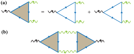
Figure 1: (Color online) (a) Diagrams for the nonlinear susceptibility $\Gamma$. The black (dark) wavy line denotes a vector potential coupled to a current vertex and the light (green) wavy lines denote scalar potentials coupled charge vertices. (b) Diagram for the drag transconductivity. Interlayer screened Coulomb interactions ( green (light) wave lines representing interlayer Coulomb interactions $U(q,\omega)$ link the two triangle nonlinear susceptibility diagrams.

The central quantity in the Coulomb drag problem Oreg ; Jauho is the nonlinear susceptbility $\bm{\Gamma}(\bm{q},\omega,B)$ [See Fig. 1(a)]. We now derive an expression for this quantity that is valid for graphene in a magnetic field. The Green’s function in Fig. 1(a) is

$$G_{n,s,X}(\varepsilon)=\frac{|n,s,X\rangle\langle n,s,X|}{\varepsilon-\varepsilon_{s,n}+i/2\tau},$$ (1)

where $|n,s,X\rangle$ is an eigenstate eigen_remark and $\tau$ is its lifetime. The three vertices in the nonlinear susceptibility diagram Fig. 1(a) contain matrix elements of the current and charge density operators between different LL wavefunctions. In a continuum model, the eigenstates are spinors with components on both honeycomb sublattices. The current and charge density matrix elements are:

$$\langle n_{2},s_{2},X_{2}|j_{x}|n_{3},s_{3},X_{3}\rangle=ev\delta_{X_{2},X_{3}}$$

$$\times\mathcal{N}_{n_{2}}\mathcal{N}_{n_{3}}\left[s_{2}\delta_{n_{2}-1,n_{3}}+s_{3}\delta_{n_{2},n_{3}-1}\right],$$ (2)

$$\langle n_{1},s_{1},X_{1}|e^{i\bm{q}\cdot\bm{r}}|n_{2},s_{2},X_{2}\rangle=\delta_{X_{1},X_{2}+q_{y}\ell_{B}^{2}}e^{iq_{x}(X_{1}+X_{2})/2}$$

$$\times\mathcal{N}_{n_{1}}\mathcal{N}_{n_{2}}\left[F_{n_{1},n_{2}}(\bm{q})+s_{1}s_{2}F_{n_{1}-1,n_{2}-1}(\bm{q})\right],$$ (3)

where $\mathcal{N}_{n}=\delta_{n,0}+(1-\delta_{n,0})/\sqrt{2}$ is a normalization factor, and we have defined

$$F_{n_{1},n_{2}}(\bm{q})=\sqrt{\frac{n_{<}!}{n_{>}!}}e^{-q^{2}\ell_{B}^{2}/4}L_{n_{<}}^{n_{>}-n_{<}}\left(\frac{q^{2}\ell_{B}^{2}}{2}\right)\left(\frac{i\tilde{q}\ell_{B}}{\sqrt{2}}\right)^{n_{>}-n_{<}}.$$ (4)

In Eq. (3), $q=|\bm{q}|$, $\tilde{q}=q_{x}+iq_{y}$, $n_{>}=\mathrm{max}(n_{1},n_{2})$, $n_{<}=\mathrm{min}(n_{1},n_{2})$, and $L_{n}^{\alpha}$ is the generalized Laguarre polynomial of degree $n$. Evaluating Fig. 1(a) using the standard Matsubara Feynman diagram technique and Eqs. (1)-(4), we obtain the following compact expression for the nonlinear susceptibility:

$$\bm{\Gamma}(\bm{q},\omega,\bm{B})=2\ell_{B}^{2}\bm{q}\times\hat{\bm{B}}\,\mathrm{Im}\;\Pi({q},\omega,B),$$ (5)

where $\hat{\bm{B}}$ is the direction of the magnetic field,

$$\Pi({q},\omega,B)=-\frac{g}{2\pi\ell_{B}^{2}}\sum_{n_{1},n_{2}=0}^{\infty}\sum_{s_{1},s_{2}=\pm}$$ (6)

$$\frac{f_{s_{1},n_{1}}-f_{s_{2},n_{2}}}{\omega+s_{1}\varepsilon_{n_{1}}-s_{2}\varepsilon_{n_{2}}+i/2\tau}\;\;\mathcal{F}_{s_{1},s_{2}}(q\ell_{B},n_{1},n_{2}),$$

$g=4$ accounts for the spin and valley degeneracy, and $f_{s,n}$ is the Fermi occupation factor for the $(n,s,X)$ LL. The form factor $\mathcal{F}$ in Eq. (6) is

$$\mathcal{F}_{s_{1},s_{2}}(x,n_{1},n_{2})=\frac{e^{-x^{2}/2}}{4}\left(\frac{x^{2}}{2}\right)^{n_{>}-n_{<}}$$

$$\times\left[s_{1}\sqrt{\frac{n_{<}!}{n_{>}!}}L^{n_{>}-n_{<}}_{n_{<}}\left(\frac{x^{2}}{2}\right)\right.$$

$$\left.+s_{2}\sqrt{\frac{(n_{<}-1)!}{(n_{>}-1)!}}L^{n_{>}-n_{<}}_{n_{<}-1}\left(\frac{x^{2}}{2}\right)\theta\left(n_{<}-1\right)\right]^{2},$$ (7)

where $\theta(x)=1$ for $x\geq 0$ and $0$ otherwise. The quantity $\Pi$ in Eq. (6) is the polarization function of Dirac fermions in a perpendicular quantizing magnetic field Polarpapers . The nonlinear susceptibility $\bm{\Gamma}$ is therefore directly proportional to the imaginary part of the polarization function, as in the conventional 2DEG case with a single non-chiral parabolic band Bonsager .

This finding might seem surprising since the $\Gamma(q,\omega)\propto\mathrm{Im}\,\Pi(q,\omega)$ property of a conventional 2DEG Oreg ; Jauho does not apply to the nonlinear susceptibility of graphene Dragpaper1 in the absence of a magnetic field. This difference can be explained by noting that while the energy dispersions of the conventional 2DEG and graphene are different at $B=0$, both have dispersionless Landau levels at strong $B$. We therefore conjecture that, in a strong magnetic field when disorder does not appreciably mix Landau levels, the simple relationship $\Gamma\propto\mathrm{Im}\,\Pi(q,\omega)$ is a universal feature of all clean two-dimensional electron systems, regardless of their energy dispersions. In such a case the nonlinear susceptibility is, like the polarization function, dominated by inelastic inter-LL transitions of electrons from one localized LL orbit to another localized LL orbit.

Another remarkable distinction of the strong magnetic field is brought to light by examining the drag resistivity at the CNP. The nonlinear susceptibility of graphene in the absence of a magnetic field was first evaluated in Ref. Tse_GDrag . Making use of the electron-hole symmetry of the bands and time-reversal invariance it is straightforward to show that, at $B=0$, $\bm{\Gamma}({q},\omega)$ is an odd function of the chemical potential $\mu$. When the chemical potential is at the Dirac point, $\Gamma=0$ because the two diagrams comprising Fig. 1(a) exactly cancel. Drag therefore vanishes when either layer is charge neutral. At high temperatures this behavior has indeed been observed experimentally Tutuc_exp1 ; Geim_drag1 . In the presence of a strong magnetic field, on the other hand, the nonlinear susceptibility Eq. (5) is an even function of $\mu$, as we prove below.

First, we note that electron-hole symmetry is preserved for the $s=\pm$ LLs so that $f_{s,n}(\mu)=1-f_{-s,n}(-\mu)$, and that the form factor in Eq. (7) is invariant under $s_{1}\to-s_{1}$ and $s_{2}\to-s_{2}$. Next we can interchange the labels $n_{1}\leftrightarrow n_{2}$, $s_{1}\leftrightarrow s_{2}$ to conclude that $\Pi({q},\omega,B)$ is invariant under $\mu\to-\mu$. It then follows from Eq. (5) that $\bm{\Gamma}(\bm{q},\omega,\bm{B};\mu)=-\bm{\Gamma}(-\bm{q},\omega,\bm{B};-\mu)=\bm{\Gamma}(\bm{q},\omega,\bm{B};-\mu)$. The final identity requires the observation that the form factors in Eq. (7) depend on $q=|\bm{q}|$ only. Therefore, the contributions from the two diagrams in Fig. 1(a) do not cancel at $\mu=0$ as they do in the absence of broken time-reversal symmetry. Drag can be finite even when one of the layers is charge neutral.

The interlayer transconductivity diagrams Oreg ; Jauho yield the drag conductivity [Fig. 1(b)]

$$\sigma_{\alpha\beta}^{\mathrm{D}}=\frac{e^{2}}{16\pi\hbar k_{\mathrm{B}}T}\sum_{q}\int_{-\infty}^{+\infty}\frac{\mathrm{d}\omega}{\mathrm{sinh}^{2}(\omega/2k_{\mathrm{B}}T)}$$

$$\times{\Gamma}_{\alpha}^{\mathrm{L}}(\bm{q},\omega,\bm{B}){\Gamma}_{\beta}^{\mathrm{R}}(\bm{q},\omega,-\bm{B})|U(q,\omega,B)|^{2},$$ (8)

where the superscripts ‘L’ and ‘R’ (left and right) label the two layers, and $U(q,\omega,B)$ is the screened interlayer Coulomb interaction in the random phase approximation RPA . The Coulomb interaction strength in graphene is characterized by the dimensionless coupling constant $\alpha_{\mathrm{G}}=e^{2}/(\epsilon\hbar v)$, where $\epsilon$ is an effective dielectric constant which we view as a parameter that can be altered by changing the sheet’s dielectric environment USupp . The quantity measured in most Coulomb drag experiments is the drag resistivity, which can be obtained by inverting the four component (two layers each with two directions) conductivity tensor $\overleftrightarrow{\sigma}$ of the bilayer , $\overleftrightarrow{\rho}=(\overleftrightarrow{\sigma})^{-1}$. The conductivity tensor becomes diagonal in Cartesian labels when $\hat{x}$ and $\hat{y}$ components are replaced by left and right handed components ($\hat{x}\pm i\hat{y}$) components. It simplifies further in the special case of identical left and right sheets since parallel flow and counterflow are then decoupled.

For the general case we introduce the definitions:

$$\mathcal{S}_{xx} = {(\sigma_{xx}^{\mathrm{D}})^{2}-\sigma_{xx}^{\mathrm{L}}\sigma_{xx}^{\mathrm{R}}+\sigma_{xy}^{\mathrm{L}}\sigma_{xy}^{\mathrm{R}}},$$ (9)

$$\mathcal{S}_{xy} = {\sigma_{xy}^{\mathrm{L}}\sigma_{xx}^{\mathrm{R}}+\sigma_{xx}^{\mathrm{L}}\sigma_{xy}^{\mathrm{R}}},$$ (10)

where $\sigma_{xx}^{\mathrm{L,R}}$ and $\sigma_{xy}^{\mathrm{L,R}}$ are the longitudinal and Hall conductivities in the individual layers. Because the Hall drag conductivity $\sigma_{xy}^{\mathrm{D}}$ vanishes due to the odd momentum dependence of $\bm{\Gamma}\propto\bm{q}\times\hat{\bm{B}}$ in Eq. (5), the general drag resistivity tensor expression simplifies to

$$\rho_{\alpha\beta}^{\mathrm{D}}=\sigma_{xx}^{\mathrm{D}}{\mathcal{S}_{\alpha\beta}}/({\mathcal{S}_{xx}^{2}+\mathcal{S}_{xy}^{2}}),$$ (11)

where $\alpha,\beta=x$ or $y$. In 2DEG systems, the Hall drag resistivity is negligible for $\omega_{\mathrm{c}}\tau\ll 1$, where $\omega_{\mathrm{c}}$ is the cyclotron frequency Oreg ; Hu_Hall . In strong magnetic fields, the Hall drag resistivity is finite and can be significant, arising from the longitudinal drag combined with the intralayer Hall responses $\sigma_{xy}^{\mathrm{L,R}}$. From Eq. (10), we observe that the Hall drag $\rho_{xy}^{\mathrm{D}}$ is comparable to the longitudinal drag $\rho_{xx}^{\mathrm{D}}$ in magnitude except when (1) both layers are characterized by well-formed quantum Hall plateaus such that the longitudinal conductivities vanish $\sigma_{xx}^{\mathrm{L,R}}=0$; or (2), since $\sigma^{L,R}_{xx}(\mu)=\sigma^{L,R}_{xx}(-\mu)$ and $\sigma_{xy}^{L,R}(\mu)=-\sigma_{xy}^{L,R}(-\mu)$, the two layers have opposite carrier densities Geim_drag1 ; Geim_drag2 ; Tutuc_exp1 .

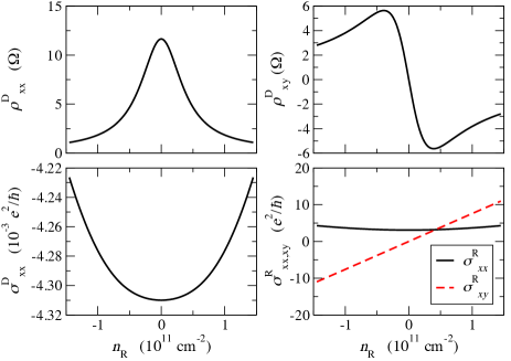
Figure 2: (Color online) Longitudinal (a) and Hall (b) drag resistivities of double-layer graphene as a function of right-layer electron density $n_{\mathrm{R}}$ for $n_{\mathrm{L}}=0$, $B=0.5\,\mathrm{T}$, $T=300\,\mathrm{K}$, $d=30\,\AA$, $1/2\tau=1\,\mathrm{meV}$, and $\alpha_{\mathrm{G}}=0.4$. Panel (c) shows the corresponding drag conductivities and (d) the longitudinal and Hall conductivities.

Dirac-Point Drag and Hall Drag.— In the following we present numerical results for the drag resistivities evaluated from Eqs. (8)-(11). We employ the Thomas-Fermi approximation in the screened interlayer Coulomb interaction USupp . We first keep the density of one layer ($n_{L}$) fixed at the CNP and vary the density of the other layer ($n_{R}$). Fig. 2(a) shows the longitudinal drag resistivity as a function of density in the vicinity of the CNP for $B=0.5\,\mathrm{T}$. The most important feature we find is that $\rho_{xx}^{\mathrm{D}}$ has its maximum value at the simultaneous CNP $n_{\mathrm{L,R}}=0$. Away from the CNP, $\rho_{xx}^{\mathrm{D}}$ is an even function of $n_{R}$ and decreases with its magnitude. In Fig. 2(b) we show the Hall drag resistivity $\rho_{xy}^{\mathrm{D}}$, which is an odd function of $n_{R}$. The magnitude of $\rho_{xy}^{\mathrm{D}}$ rises sharply from zero away from the simultaneous CNP and then drops gradually as the layer’s carrier density is further increased. In Fig. 2(c)-(d) we also depict the behavior of the drag conductivity as well as the R layer’s longitudinal and Hall conductivities. As shown in Fig. 2(c), the magnitude of the drag conductivity $|\sigma_{xx}^{\mathrm{D}}|$ decreases with density. We note that the sign of the drag conductivity is negative and its value is three orders of magnitude smaller than the longitudinal and Hall conductivities $\sigma_{xx,xy}$, which results in a positive sign of the drag resistivity $\rho_{xx}^{\mathrm{D}}$.

Fig. 3 shows the dependence of $\rho_{xx}^{\mathrm{D}}$ on $n_{\mathrm{L}}$ and $n_{\mathrm{R}}$. We observe that $\rho_{xx}^{\mathrm{D}}$ is positive in the two quadrants of electron-hole drag where the ‘L’ and ‘R’ carriers have opposite polarities, and mostly negative in the quadrants of electron-electron and hole-hole drag, with $\rho_{xx}^{\mathrm{D}}<0$ except near the simultaneous CNP at $n_{\mathrm{L,R}}\lesssim 10^{10}\,\mathrm{cm}^{-2}$. These features are in good agreement with the latest experiment Kim_exp2 performed under strong magnetic fields. With the exception of the CNP vicinity, the signs of magnetodrag for the cases of same and opposite carrier polarities depicted in Fig. 3 are the same as that in the zero-field case Tse_GDrag ; Dragpaper1 ; Tutuc_exp1 ; Geim_drag1 and consistent with magnetodrag in conventional 2DEG Bonsager . Unlike conventional 2DEG however, which would exhibit no drag when the carrier density is tuned to zero in one of the layers, double-layer graphene exhibits a distinctive finite magnetodrag at the simultaneous CNP due to the presence of a Dirac sea of electrons and a gapless energy dispersion. While interlayer energy transfer has been proposed as a possible mechanism Dragpaper6 to explain the finite drag resistivity at the CNP observed in zero-field experiments, we emphasize that such a mechanism is not necessary to explain the finite positive drag at CNP in the presence of a magnetic field, as our findings have demonstrated.

The fact that $\sigma^{D}_{xx}$ is non-zero and has a negative sign at $\mu=0$ can be physically explained as follows. Let us assume that the magnetic field is in the $z$-direction and the electric field is applied to the active layer in the positive $y$-direction. Assuming that the longitudinal components are negligible compared to the transverse components of the intralayer $\sigma^{\mathrm{L,R}}$, this implies that particle currents in the active layer are in the positive $x$-direction (independent of whether they are electrons or holes). Therefore, the drag force on the passive layer is in the positive $x$-direction. This acts like an effective electric field in the positive (negative) $x$-direction for holes (electrons), which results in an “$\mathbf{E}$”$\times\mathbf{B}$ drift of the holes (electrons) in the negative (positive) $y$-direction. Hence, for both electrons and holes, the electric current in the passive layer is in the negative $y$-direction; i.e., $\sigma^{D}_{xx}<0$. At finite temperature the drag currents due to thermally excited electrons and holes reinforce each other and do not cancel. The drag conductivity is an even function of the chemical potential, consistent with the evenness of $\Gamma$ discussed above.

Since a negative longitudinal conductivity results in a thermodynamic instability, our findings beg an important question: does a negative drag conductivity also implies a thermodynamic instability? The condition for thermodynamic stability is that the conductivity matrix be positive definite. In the presence of a magnetic field, the Hall conductivities render the conductivity matrix $\overleftrightarrow{\sigma}$ anti-symmetric. For an arbitrary square matrix that is not necessarily symmetric, the positive definiteness condition depends on the positivity of the determinant of the symmetric part of the matrix only Johnson . It follows that the Hall conductivities $\sigma_{xy}^{\mathrm{L,R}}$ drop out and the resulting determinant is given by $\sigma_{xx}^{\mathrm{L}}\sigma_{xx}^{\mathrm{R}}-(\sigma_{xx}^{\mathrm{D}})^{2}$, which is positive definite, sharing the same expression with the $B=0$ case.

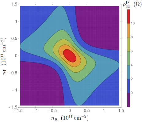
Figure 3: (Color online) Longitudinal drag resistivity as a function of right-layer electron density $n_{\mathrm{R}}$ and left-layer electron density $n_{\mathrm{L}}$ for the same values of $B,T,d$, and $\alpha_{\mathrm{G}}$ as in Fig. 2.

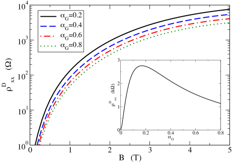
Figure 4: (Color online) Longitudinal drag resistivity at the simultaneous CNP $n_{\mathrm{L}}=n_{\mathrm{R}}=0$ as a function of magnetic field for different values of interaction coupling $\alpha_{\mathrm{G}}=0.2,0.4,0.6,0.8$. Inset: The same quantity as a function of $\alpha_{\mathrm{G}}$ at a fixed magnetic field $B=3\,\mathrm{T}$. $T$ and $d$ are the same as in previous figures.

Finally, we have calculated the longitudinal drag resistivity $\rho_{xx}^{\mathrm{D}}$ at the simultaneous CNP as a function of the magnetic field for different values of the interaction parameter $\alpha_{\mathrm{G}}$. Fig. 4 shows that $\rho_{xx}^{\mathrm{D}}$ is highly sensitive to changing magnetic field strength, increasing to several $\mathrm{k}\Omega\mathrm{s}$ over a few teslas. It also shows that changing the electron-electron interaction strength $\alpha_{\mathrm{G}}$ from $0.2$ to $0.8$ counterintuitively decreases $\rho_{xx}^{\mathrm{D}}$. This finding can be explained by examining the $\alpha_{G}$ dependence of the interlayer interaction $U(q,\omega,B)$ USupp . Unlike the single layer case where the screened interaction $V\sim\alpha_{\mathrm{G}}/(1+\alpha_{\mathrm{G}})$ monotonically increases with $\alpha_{\mathrm{G}}$, the screened interlayer interaction of a bilayer $U\sim\alpha_{\mathrm{G}}/(1+\alpha_{\mathrm{G}}^{2})$ decreases for large $\alpha_{\mathrm{G}}$. This behavior is fully reflected in the drag resistivity as a function of $\alpha_{\mathrm{G}}$ depicted in the inset of Fig. 4.

In summary, we find that the magneto-drag resistivity of graphene double layers has a maximum and that the Hall drag resistivity vanishes at the simultaneous CNP. The Hall drag resistivity is however comparable to the longitudinal resistivity at nearby densities, even though the Hall drag conductivity vanishes. Our theory accounts for momentum transfer due to interactions between density-fluctuations in the two layers, but does not account for strong correlations or address all possible scenarios that have been raised Geim_drag2 ; Schutt in connection with graphene double-layer magnetodrag. The physics we explore must however contribute significantly to any magnetodrag measurements.

Work at Alabama (WKT and JNH) was supported by startup and Research Grants Committee funds from the University of Alabama. AHM was supported by the DOE Division of Materials Sciences and Engineering under grant DE-FG02-ER45958 and by the Welch foundation under grant TBF1473. BYKH acknowledges support from the University of Akron for a Professional Development Leave.

References

- (1) A. H. Castro Neto, F. Guinea, N. M. R. Peres, K. S. Novoselov, and A. K. Geim, Rev. Mod. Phys. 81, 109 (2009).
- (2) S. Das Sarma, S. Adam, E. H. Hwang, and E. Rossi, Rev. Mod. Phys. 83, 407 (2011).
- (3) B. N. Narozhny and A. Levchenko, Rev. Mod. Phys. 88, 025003 (2016).
- (4) K. S. Novoselov, A. Mishchenko, A. Carvalho, and A. H. Castro Neto, Science 353, 461 (2016)
- (5) A.K. Geim and I.V. Grigorieva, Nature 499, 419 (2013).
- (6) W.-K. Tse, B. Y.-K. Hu, and S. Das Sarma, Phys. Rev. B 76, 081401(R) (2007).
- (7) M. I. Katsnelson, Phys. Rev. B 84, 041407(R) (2011).
- (8) E. H. Hwang, R. Sensarma, and S. Das Sarma, Phys. Rev. B 84, 245441 (2011).
- (9) N. M. R. Peres, J. M. B. Lopes dos Santos, and A. H. Castro Neto, EPL 95 18001 (2011).
- (10) B. N. Narozhny, M. Titov, I. V. Gornyi, P. M. Ostrovsky, Phys. Rev. B 85, 195421 (2012).
- (11) M. Carrega, T. Tudorovskiy, A. Principi, M. I. Katsnelson, and M. Polini, New J. Phys. 14, 063033 (2012).
- (12) J. C. W. Song and L. S. Levitov, Phys. Rev. Lett. 109, 236602 (2012).
- (13) R. Geick, C. H. Perry, and G. Rupprecht, Phys. Rev. 146, 543 (1966).
- (14) S. Kim, I. Jo, J. Nah, Z. Yao, S. K. Banerjee, and E. Tutuc, Phys. Rev. B 83, 161401(R) (2011); S. Kim and E. Tutuc, Solid State Comm. 152, 1283 (2012).
- (15) R. V. Gorbachev, A. K. Geim, M. I. Katsnelson, K. S. Novoselov, T. Tudorovskiy, I. V. Grigorieva, A. H. MacDonald, K. Watanabe, T. Taniguchi, and L. A. Ponomarenko, Nature Phys. 8, 896 (2012).
- (16) M. Titov, R. V. Gorbachev, B. N. Narozhny, T. Tudorovskiy, M. Schutt, P. M. Ostrovsky, I. V. Gornyi, A. D. Mirlin, M. I. Katsnelson, K. S. Novoselov, A. K. Geim, and L. A. Ponomarenko, Phys. Rev. Lett. 111, 166601 (2013).
- (17) J. Li, T. Taniguchi, K. Watanabe, J. Hone, A. Levchenko, and C. Dean, Phys. Rev. Lett. 117, 046802 (2016).
- (18) K. Lee, J. Xue, D. C. Dillen, K. Watanabe, T. Taniguchi, and E. Tutuc, Phys. Rev. Lett. 117, 046803 (2016).
- (19) J. I. A. Li, T. Taniguchi, K. Watanabe, J. Hone, and C. R. Dean, Nat. Phys. 13, 751 (2017).
- (20) X. Liu, K. Watanabe, T. Taniguchi, B. I. Halperin, and P. Kim, arXiv:1608.03726 (2016).
- (21) X. Liu, L. Wang, K. C. Fong, Y. Gao, P. Maher, K. Watanabe, T. Taniguchi, J. Hone, C. Dean, and P. Kim, Phys. Rev. Lett. 119, 056802 (2017).
- (22) A. Kamenev and Y. Oreg, Phys. Rev. B 52, 7516 (1995).
- (23) K. Flensberg, B. Y.-K. Hu, A.-P. Jauho, and J. M. Kinaret, Phys. Rev. B 52, 14761 (1995).
- (24) For compactness and uniformity, we use the same notation and for all LLs including , with and .
- (25) K. Shizuya, Phys. Rev. B 75, 245417 (2007); R. Roldan, J.-N. Fuchs, and M. O. Goerbig, Phys. Rev. B 80, 085408 (2009); C. H. Yang, F. M. Peeters, and W. Xu, Phys. Rev. B 82, 075401 (2010); P. K. Pyatkovskiy and V. P. Gusynin, Phys. Rev. B 83, 075422 (2011).
- (26) M. C. Bønsager, K. Flensberg, B. Y.-K. Hu, and A.-P. Jauho, Phys. Rev. Lett. 77, 1366 (1996); Phys. Rev. B 56, 10314 (1997).
- (27) In strong magnetic fields, it is an intricate task to take into account the effect of screening properly covering a reasonably wide range of filling factors. The random phase approximation (RPA) is commonly adopted Oppen ; Nazarov for the interlayer screened Coulomb potential to capture the main features of screening under strong magnetic fields in which fractional quantum Hall effect is not yet developed.
- (28) See the included Supplemental Material for details of the interlayer Coulomb interaction in the statically screened random phase approximation.
- (29) I. V. Gornyi, A. D. Mirlin, and F. von Oppen, Phys. Rev. B 70, 245302 (2004).
- (30) A.V. Khaetskii and Yu.V. Nazarov, Phys. Rev. B 59, 7551 (1999).
- (31) B. Y.-K. Hu, Phys. Scr. 1997, 170 (1997).
- (32) C. R. Johnson, Amer. Math. Monthly 77, 259 (1970).
- (33) M. Schutt, P. M. Ostrovsky, M. Titov, I. V. Gornyi, B. N. Narozhny, and A. D. Mirlin, Phys. Rev. Lett. 110, 026601 (2013).