Waveguides for Rydberg excitons in Cu${}_{\text{2}}$O from strain traps

Abstract

We investigate the formation of waveguides for Rydberg excitons in Cu${}_{\text{2}}$O from cylindrical stressors as alternatives to optical traps. We show that the achievable potential depths can easily reach the $\mathrm{meV}$ and the trap frequencies the $\mathrm{GHz}$ regimes. For Rydberg excitons, we find that it is sufficient to consider only the shift of the band gap, whereas the excitonic binding energies remain almost unchanged.

I Introduction

Excitons, bound states of an electron and a positively charged hole, are the fundamental optical excitations in a semiconductor. Cuprous oxide (Cu${}_{\text{2}}$O) was the first material in which the formation of excitons with principal quantum numbers up to $n=8$ was experimentally demonstrated Gross and Karryev (1952); Gross (1956). In recent years, the variety of observed excitonic states has increased greatly Kazimierczuk et al. (2014); Thewes et al. (2015); Schöne et al. (2016), including highly excited states of principal quantum numbers up to $n=25$ and orbital quantum numbers of $\ell=5$. These highly excited states do already show all the hallmarks of the Rydberg blockade Kazimierczuk et al. (2014) as well as signs of quantum coherence Grünwald et al. (2016).

Strain potentials from inhomogeneous strain fields alter the band structure of the crystal and can generate effective trapping potentials. They have been used and extensively investigated in the pursuit of exciton condensation in Cu${}_{\text{2}}$O Trauernicht et al. (1986); Snoke and Negoita (2000); Naka and Nagasawa (2002, 2004); Yoshioka et al. (2011); Stolz et al. (2012); Schwartz et al. (2012). Due to the long lifetime of the 1S paraexciton of its yellow exciton series ($\sim$\mathrm{\SIUnitSymbolMicro s}$$), most research has hitherto been focused on the yellow 1S para- and orthoexcitons. Strain influence on the yellow P-excitons has been investigated in thin filmsIwamitsu et al. (2014). In comparison to the dipole traps frequently used in atomic physics, strain traps potentially offer a greater variety of achievable trap geometries, as the shape of the trap depends strongly on the shape of the stressor, the stress applied to it, the excitonic state in question as well as the orientation of the crystal relative to the stress Naka and Nagasawa (2004); Sandfort et al. (2011). Furthermore, the achievable potential depths ($\sim$\mathrm{meV}$$) and trap frequencies ($\sim$\mathrm{GHz}$$) are much higher than those of the atomic dipole traps ($\sim$\mathrm{\SIUnitSymbolMicro eV}$$ and $\sim$\mathrm{MHz}$$) Grimm et al. (2000).

Excitonic traps may be a useful experimental tool for the investigation of exciton-exciton interactions and many-body effects in exciton populations. The 1D potential landscapes induced by cylindrical stressors offer a positional control over the exciton populations in two dimensions and could pave the way for the investigation of 1D many-body interactions between excitons.

In this article, we investigate the modification of the Rydberg exciton resonances in Cu${}_{\text{2}}$O under the influence of strain from a cylindrical stressor (see Fig. 1). The strain field $\bm{\epsilon}(\bm{r})$ will be calculated using Hertzian contact theory M’Ewen (1949); Manghnani et al. (1974), while the band Hamiltonian derived by Suzuki and Hensel Suzuki and Hensel (1974) will be employed in order to describe the strain dependence of the hole motion, from which the band-gap shifts $\Delta E_{g}(\bm{r})$ can be obtained. The shifts of the binding energies will be calculated using a two-band model similar to Ref. Schöne et al. (2016), generalised to anisotropic band structures.

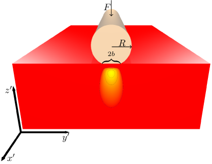
Figure 1: Schematic cross section of the proposed geometry with a cylindrical stressor acting on a Cu${}_{\text{2}}$O crystal with line load $F$ (force per unit length) and the resulting trapping potential. $b$ denotes the half width of the contact area.

The article is organised as follows. Section II introduces the band and strain Hamiltonians used in this study. In Sec. III the strain fields and the resulting band-gap shifts will be calculated for certain geometries and stresses. The influence on the excitonic binding energies will be discussed in Sec. IV, and Sec. V presents the conclusion and an outlook.

II Electron and hole motion under the influence of strain

We begin with a brief review of the band structure of Cu${}_{\text{2}}$O under the influence of strain. Without spin, the uppermost valence band of Cu${}_{\text{2}}$O has $\Gamma^{+}_{5}$-symmetry at the zone center, which splits into a twofold degenerate $\Gamma^{+}_{7}$- and a fourfold degenerate $\Gamma^{+}_{8}$-band under the influence of spin-orbit interaction. An effective $6\times 6$-Hamiltonian for these valence bands up to second order in the hole momentum $\hbar\bm{k}_{h}$ and first order in the components of the strain tensor $\epsilon_{ij}$ ($i,j=x,y,z$) can be constructed based on group-theoretical considerations Suzuki and Hensel (1974). It takes the form $\mathcal{H}_{v}(\bm{k}_{h},\bm{\epsilon})=\mathcal{H}_{so}+\mathcal{H}_{\bm{k}_{h}}+\mathcal{H}_{\bm{\epsilon}}$ where $\mathcal{H}_{so}=-\frac{\Delta}{3}(2+\bm{I}\cdot\bm{\sigma})$ describes the $\bm{k}_{h}$-independent spin-orbit splitting, $\bm{I}$ denotes the vector of the angular-momentum matrices for $I=1$, $\bm{\sigma}$ the vector of the Pauli matrices and $\Delta$ the spin-orbit splitting. Note that our definition of the spin-orbit splitting guarantees that the band edge of the $\Gamma^{+}_{7}$ valence band is located at the origin of the energy scale.

The $\bm{k}_{h}$-dependent part of the Hamiltonian is given by

$$\mathcal{H}_{\bm{k}_{h}}=\frac{\hbar^{2}}{2m_{e}}\bigg{\{}\left(A_{1}+B_{1}\bm{I}\cdot\bm{\sigma}\right)\bm{k}_{h}^{2}$$

$$+\left[A_{2}\left(I_{x}^{2}-\frac{1}{3}\bm{I}^{2}\right)+B_{2}\left(I_{x}\sigma_{x}-\frac{1}{3}\bm{I}\cdot\bm{\sigma}\right)\right]k_{x,h}^{2}+\mathrm{c.p.}$$

$$+\left[A_{3}(I_{x}I_{y}+I_{y}I_{x})+B_{3}(I_{x}\sigma_{y}+I_{y}\sigma_{x})\right]\{k_{x,h}k_{y,h}\}+\mathrm{c.p.}\bigg{\}}$$

where $\mathrm{c.p.}$ denotes cyclic permutations, $\{k_{i}k_{j}\}=(k_{i}k_{j}+k_{j}k_{i})/2$ is the symmetric product of momenta, and the $A_{i}$ and $B_{i}$ are dimensionless material constants. Values for all material properties of Cu${}_{\text{2}}$O used in this work can be found in Table 1. In the absence of external electromagnetic fields, the symmetric, cartesian strain tensor $\bm{\epsilon}$ with components $\epsilon_{ij}$ transforms according to the same reducible representation of the point group $O_{h}$ as $k_{i}k_{j}$, hence the strain Hamiltonian for the valence band has an analogous form to $\mathcal{H}_{\bm{k}_{h}}$

$$\mathcal{H}_{\bm{\epsilon}}=\left(D_{1}+E_{1}\bm{I}\cdot\bm{\sigma}\right)\operatorname{Tr}(\bm{\epsilon})$$

$$+\left[D_{2}\left(I_{x}^{2}-\frac{1}{3}\bm{I}^{2}\right)+E_{2}\left(I_{x}\sigma_{x}-\frac{1}{3}\bm{I}\cdot\bm{\sigma}\right)\right]\epsilon_{xx}+\mathrm{c.p.}$$

$$+\left[D_{3}\left(I_{x}I_{y}+I_{y}I_{x}\right)+E_{3}\left(I_{x}\sigma_{y}+I_{y}\sigma_{x}\right)\right]\epsilon_{xy}+\mathrm{c.p.}$$ (2)

with the deformation potentials $D_{i}$ and $E_{i}$. The $E_{i}$ are assumed to be negligible, as is usually done in the literature Naka and Nagasawa (2004); Sandfort et al. (2011).

The equivalent effective Hamiltonian for the $\Gamma^{+}_{6}$ conduction band is given by the $2\times 2$-matrix

$$\mathcal{H}_{c}(\bm{k}_{e},\bm{\epsilon})=E_{g}+\frac{\hbar^{2}}{2m_{e}}A_{4}\bm{k}_{e}^{2}+C_{1}\operatorname{Tr}(\bm{\epsilon}).$$ (3)

A spatially homogeneous strain preserves the inversion symmetry as well as the time-reversal symmetry. Thus, the twofold degeneracy over the whole Brillouin zone of both the $\Gamma^{+}_{7}$ valence band and the $\Gamma^{+}_{6}$ conduction band is maintained. As long as the strain field is approximately constant across the exciton volume, the assumption of spatial homogeneity is justified.

The kinetic energy of the relative electron-hole motion $\mathcal{H}_{r}(\bm{k},\bm{\epsilon})=\mathcal{H}_{c}(\bm{k},\bm{\epsilon})\otimes\operatorname{Id}_{v}-\operatorname{Id}_{c}\otimes\mathcal{H}_{v}(\bm{k},\bm{\epsilon})$ for vanishing center-of-mass momentum $\hbar\bm{K}=0$ is thus given by the $12\times 12$ matrix

$$\mathcal{H}_{r}(\bm{k},\bm{\epsilon})=\operatorname{Id}_{c}\otimes(E_{g}-\mathcal{H}_{v}(\bm{k},\bm{\epsilon}))$$ (4)

with modified parameters $A_{1}\mapsto A_{1}-A_{4}$ and $D_{1}\mapsto D_{1}-C_{1}:=D^{\prime}_{1}$. Here, $\operatorname{Id}_{c}$ and $\operatorname{Id}_{v}$ denote the identity matrices in the basis of conduction-band and valence-band states, respectively. This formulation is possible as $\mathcal{H}_{c}(\bm{k}_{e},\bm{\epsilon})$ is proportional to $\operatorname{Id}_{c}$ and the terms in $\mathcal{H}_{v}(\bm{k}_{h},\bm{\epsilon})$ containing $A_{1}$ and $D_{1}$ are proportional to $\operatorname{Id}_{v}$.

The excitonic strain potential can be broken down into a pure band-gap shift $\Delta E_{g}$ and a binding energy shift $\Delta E_{b}$ induced by the deformation of the bands (for nS orthoexcitons not considered here, there is an additional strain-dependent contribution from the exchange interaction Naka and Nagasawa (2004)). The band-gap shift $\Delta E_{g}$ can be evaluated in third-order perturbation theory as

$$\Delta E_{g}(\bm{\epsilon})=-D^{\prime}_{1}\operatorname{Tr}(\bm{\epsilon})-\frac{2D_{3}^{2}\left[\epsilon_{xy}^{2}+\epsilon_{yz}^{2}+\epsilon_{zx}^{2}\right]}{3\Delta}-\frac{D_{2}^{2}\left[(\epsilon_{xx}-\epsilon_{yy})^{2}+(\epsilon_{yy}-\epsilon_{zz})^{2}+(\epsilon_{zz}-\epsilon_{xx})^{2}\right]}{9\Delta}$$

$$-\frac{D_{2}^{3}(\epsilon_{xx}+\epsilon_{yy}-2\epsilon_{zz})(\epsilon_{xx}-2\epsilon_{yy}+\epsilon_{zz})(-2\epsilon_{xx}+\epsilon_{yy}+\epsilon_{zz})}{27\Delta^{2}}+\frac{2D_{3}^{3}\epsilon_{xy}\epsilon_{yz}\epsilon_{zx}}{\Delta^{2}}$$

$$+\frac{D_{2}D_{3}^{2}~{}\left[\epsilon_{xx}(\epsilon_{xy}^{2}+\epsilon_{zx}^{2}-2\epsilon_{yz}^{2})+\epsilon_{yy}(\epsilon_{xy}^{2}+\epsilon_{yz}^{2}-2\epsilon_{zx}^{2})+\epsilon_{zz}(\epsilon_{zx}^{2}+\epsilon_{yz}^{2}-2\epsilon_{xy}^{2})\right]}{3\Delta^{2}}.$$ (5)

For a compressive strain with $\operatorname{Tr}(\bm{\epsilon})<0$, the first-order term raises the band gap and thus results in a repulsive contribution to the excitonic potential while the second-order terms lower the band gap.

Table 1: Material properties of Cu${}_{\text{2}}$O used in this work.

$D^{\prime}_{1}$	$2.1~{}$\mathrm{eV}$$	Trebin et al. (1981)	$A_{1}$	$-1.76$	Schöne et al. (2016)
$D_{2}$	$-3.9~{}$\mathrm{eV}$$		$A_{2}$	$4.519$
$D_{3}$	$1.9~{}$\mathrm{eV}$$		$A_{3}$	$-2.201$
$S_{11}$	$41.69~{}${\mathrm{TPa}}^{-1}$$	Manghnani et al. (1974)	$B_{1}$	$0.02$
$S_{12}$	$-19.36~{}${\mathrm{TPa}}^{-1}$$		$B_{2}$	$-0.022$
$S_{44}$	$82.64~{}${\mathrm{TPa}}^{-1}$$		$B_{3}$	$-0.202$
$\varepsilon_{r}$	$7.5$	Carabatos et al. (1968)	$\Delta$	$131~{}$\mathrm{meV}$$	Gross (1956)
$A_{4}$	$1.01$	Hodby et al. (1976)	$E_{g}$	$2.17208~{}$\mathrm{eV}$$	Kazimierczuk et al. (2014)

III Band-gap shifts under the influence of strain from a cylindrical stressor

For some geometries, the stress field can be calculated analytically using Hertzian contact theory. It should be noted here that Hertzian contact theory assumes elastically isotropic materials. However, comparisons between finite-element calculations and Hertzian results for germanium (whose anisotropy is stronger than that of Cu${}_{\text{2}}$O) have shown satisfying agreement Markiewicz et al. (1977).

In the case of an infinitely long cylindrical stressor in contact with a planar surface along the $x^{\prime}$ axis of the $(x^{\prime},y^{\prime})$-plane (see Fig. 1), the components of the stress tensor $\sigma_{i^{\prime}j^{\prime}}$ are given by M’Ewen (1949)^,

$$\sigma_{x^{\prime}x^{\prime}}=-2\nu\hat{\sigma}\left[m-\tilde{z}^{\prime}\right],$$ (6)

$$\sigma_{y^{\prime}y^{\prime}}=-\hat{\sigma}\left[m-2\tilde{z}^{\prime}+m\frac{\tilde{z}^{\prime 2}+n^{2}}{m^{2}+n^{2}}\right],$$ (7)

$$\sigma_{z^{\prime}z^{\prime}}=-\hat{\sigma}\left[m-m\frac{\tilde{z}^{\prime 2}+n^{2}}{m^{2}+n^{2}}\right],$$ (8)

$$\sigma_{y^{\prime}z^{\prime}}=\hat{\sigma}\left[n\frac{m^{2}-\tilde{z}^{\prime 2}}{m^{2}+n^{2}}\right],$$ (9)

$$\sigma_{x^{\prime}y^{\prime}}=\sigma_{z^{\prime}x^{\prime}}=0,$$ (10)

where $\hat{\sigma}$ is the maximum stress at the contact surface, $(\tilde{x}^{\prime},\tilde{y}^{\prime},\tilde{z}^{\prime})^{T}=b^{-1}~{}(x^{\prime},y^{\prime},z^{\prime})^{T}$ are the dimensionless coordinates of the stress field and $m$ and $n$ are given by

$$m=\frac{\tilde{z}^{\prime}}{\sqrt{2}|\tilde{z}^{\prime}|}\bigg{\{}(1-\tilde{y}^{\prime 2}+\tilde{z}^{\prime 2})$$

$$+\sqrt{(1-\tilde{y}^{\prime 2}+\tilde{z}^{\prime 2})^{2}+4\tilde{y}^{\prime 2}\tilde{z}^{\prime 2}}\bigg{\}}^{\frac{1}{2}},$$ (11)

$$n=\frac{\tilde{y}^{\prime}}{\sqrt{2}|\tilde{y}^{\prime}|}\bigg{\{}(\tilde{y}^{\prime 2}-1-\tilde{z}^{\prime 2})$$

$$+\sqrt{(1-\tilde{y}^{\prime 2}+\tilde{z}^{\prime 2})^{2}+4\tilde{y}^{\prime 2}\tilde{z}^{\prime 2}}\bigg{\}}^{\frac{1}{2}}.$$ (12)

In the case of compressive stress, the sign of $\hat{\sigma}$ coincides with the sign of $\tilde{z}^{\prime}$. The parameters $\nu=-S_{12}/S_{11}=0.464$ and $Y=1/S_{11}=23.99~{}$\mathrm{GPa}$$ (see Table 1) are Poisson’s ratio and Young’s modulus, respectively, and

$$b=2|\hat{\sigma}|R(\Theta_{\text{Cu${}_{\text{2}}$O}}+\Theta_{\text{stressor}})$$ (13)

is the half width of the contact area between stressor and crystal, with the stressor’s radius $R$ and $\Theta=(1-\nu^{2})/Y$.

The line load $F$ in Fig. 1 is related to the stress $\hat{\sigma}$ by

$$F=\frac{\hat{\sigma}\pi b}{2}=\pi\hat{\sigma}|\hat{\sigma}|R(\Theta_{\text{Cu${}_{\text{2}}$O}}+\Theta_{\text{stressor}}).$$ (14)

Due to the elastic anisotropy of Cu${}_{\text{2}}$O, the stress tensor $\bm{\sigma}(\bm{r})$ has to be transformed into the crystal coordinates $x\hat{=}[100]$, $y\hat{=}[010]$ and $z\hat{=}[001]$ first, before the strain tensor $\bm{\epsilon}(\bm{r})$ is calculated from it. The components of strain tensor and stress tensor are then connected by the compliance constants

$$\epsilon_{xx}=S_{11}\sigma_{xx}+S_{12}(\sigma_{yy}+\sigma_{zz}),$$ (15)

$$\epsilon_{yz}=S_{44}\sigma_{yz}/2$$ (16)

for the diagonal and off-diagonal components, respectively (the other components are given by cyclic permutations).

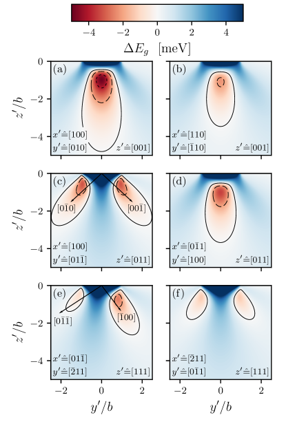
Figure 2: Band-gap shifts $\Delta E_{g}$ for a maximum stress $\hat{\sigma}=-0.65~{}$\mathrm{GPa}$$ and different orientations of the stressor relative to the crystal axes. The contour lines mark the equipotential surfaces with $\Delta E_{g}=0,-2,-4~{}$\mathrm{meV}$$ (solid, dashed, dotted). This representation does not depend on the stressor’s material properties, its radius or the line load, as long as $\hat{\sigma}$ is kept fixed.

Figure 2 shows the band-gap shifts for different orientations of the crystal relative to the stressor and a maximum stress of $\hat{\sigma}=-0.65~{}$\mathrm{GPa}$$. The spatial splitting of the band-gap potential well for a main stress in $z^{\prime}\hat{=}[011]$ direction viewed from $x^{\prime}\hat{=}[100]$ (Fig. 2 (c)) has already been observed experimentally for spherical stressors Naka and Nagasawa (2004). For the cases shown in Fig. 2 (a), (b) and (d), the potential is well approximated by a harmonic potential in $y^{\prime}$-direction, and is Morse-like along the $z^{\prime}$-direction.

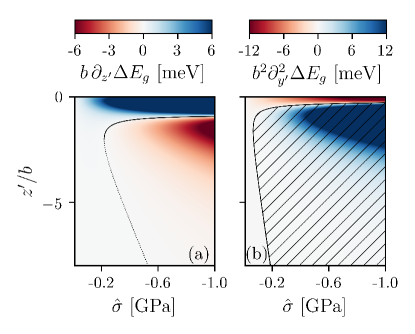
Figure 3: Derivatives of $\Delta E_{g}$ for the geometry of Fig. 2 (a) and $y^{\prime}=0$. (a): Potential gradient in $z^{\prime}$ direction . The black lines mark the potential extrema, the upper branch (solid line) corresponds to the potential minimum. (b): Second derivative in $y^{\prime}$ direction. For symmetry reasons, the first derivative does always vanish in this configuration. $\Delta E_{g}$ has a minimum in $y^{\prime}$-direction in the blue (hatched) region and a maximum in the red region.

Figure 3 shows the range of stresses in which a potential minimum can form for the arrangement of Fig. 2 (a). The limiting factor for the formation of a trap is the minimum in the $z^{\prime}$-direction, which only forms for stresses $|\hat{\sigma}|\gtrsim 0.25~{}$\mathrm{GPa}$$. From the second derivatives at the trap minimum $\bm{r}_{min}$, the trap frequencies can be calculated as

$$\omega_{x_{i}}=\sqrt{\frac{1}{M}\left.\frac{\partial^{2}\Delta E_{g}(\bm{r})}{\partial x_{i}^{2}}\right|_{\bm{r}=\bm{r}_{\min}}}$$ (17)

where $M=(A_{4}^{-1}+(2B_{1}-A_{1})^{-1})~{}m_{e}=1.55~{}m_{e}$ is the exciton mass and $x_{i}=y^{\prime},z^{\prime}$.

The trap frequencies for a stressor with $R=0.5~{}$\mathrm{mm}$$, $Y=75~{}$\mathrm{GPa}$$ and $\nu=0.3$ are shown in Fig. 4. For fixed $\hat{\sigma}$, the frequencies scale as $\omega\propto b^{-1}\propto R^{-1}(\Theta_{\text{Cu${}_{\text{2}}$O}}+\Theta_{\text{stressor}})^{-1}$. The results in Fig. 3 have been obtained by a complete diagonalisation of $\mathcal{H}_{r}(0,\bm{\epsilon})$, as the perturbation theoretical treatment introduces errors of $\sim 2~{}$\mathrm{meV}$$ at the trap minimum for $\hat{\sigma}=-1~{}$\mathrm{GPa}$$.

In order for the assumption of slowly varying strain to hold, the trap dimension should be much larger than the spatial dimension of the exciton states, i.e. $\langle r_{n,\ell}\rangle\ll b$. On the other hand, the excitonic lifetimes $\tau_{n,\ell}$ should be larger than the inverse trap frequencies $\omega^{-1}$ in order to have a meaningful definition of “trapped excitons”. The inverse trap frequencies in our numerical example are on the same order of magnitude as the lifetimes of strain-free the Rydberg excitons $\tau_{n,\ell}$ that can be estimated from the FWHM linewidths Kazimierczuk et al. (2014); Schweiner et al. (2016) $\hbar\gamma_{n,\ell}\approx\hbar/\tau_{n,\ell}$. This results in lifetimes on the order of $100\text{\,}\mathrm{ps}$ for the 15P states, compared to $\omega_{x}^{-1}\approx$500\text{\,}\mathrm{p}\mathrm{s}$$ for the parameters used in Fig. 4. As the trap frequency is inversely proportional to the trap dimension $b$, it can be tuned by the use of stressors with different radii. Additionally, strain is known to influence excitonic lifetimes in Cu${}_{\text{2}}$O Denev and Snoke (2002). To the best of our knowledge no detailed studies on the influence of strain on the lifetimes of Rydberg excitons have been performed yet, which we will leave for future work.

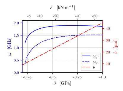
Figure 4: Trap frequencies $\omega$ and contact half width $b$ for a glass stressor with $R=0.5~{}$\mathrm{mm}$$, $Y=75~{}$\mathrm{GPa}$$ and $\nu=0.3$ in the arrangement of Fig. 2 (a).

In principle, much more intricate potential geometries can be created by corresponding stressors. As an example, Fig. 5 shows the approximate isosurfaces of the potential induced by a toroidal stressor pressed onto a Cu${}_{\text{2}}$O crystal along the $[001]$ crystal axis and viewed along the $[110]$ direction. The isosurfaces were calculated under the assumption that the stressor is locally cylindrical. The modulation arises from the varying orientation of the stressor relative to the crystal axes (see Figs. 2 (a) and (b)).

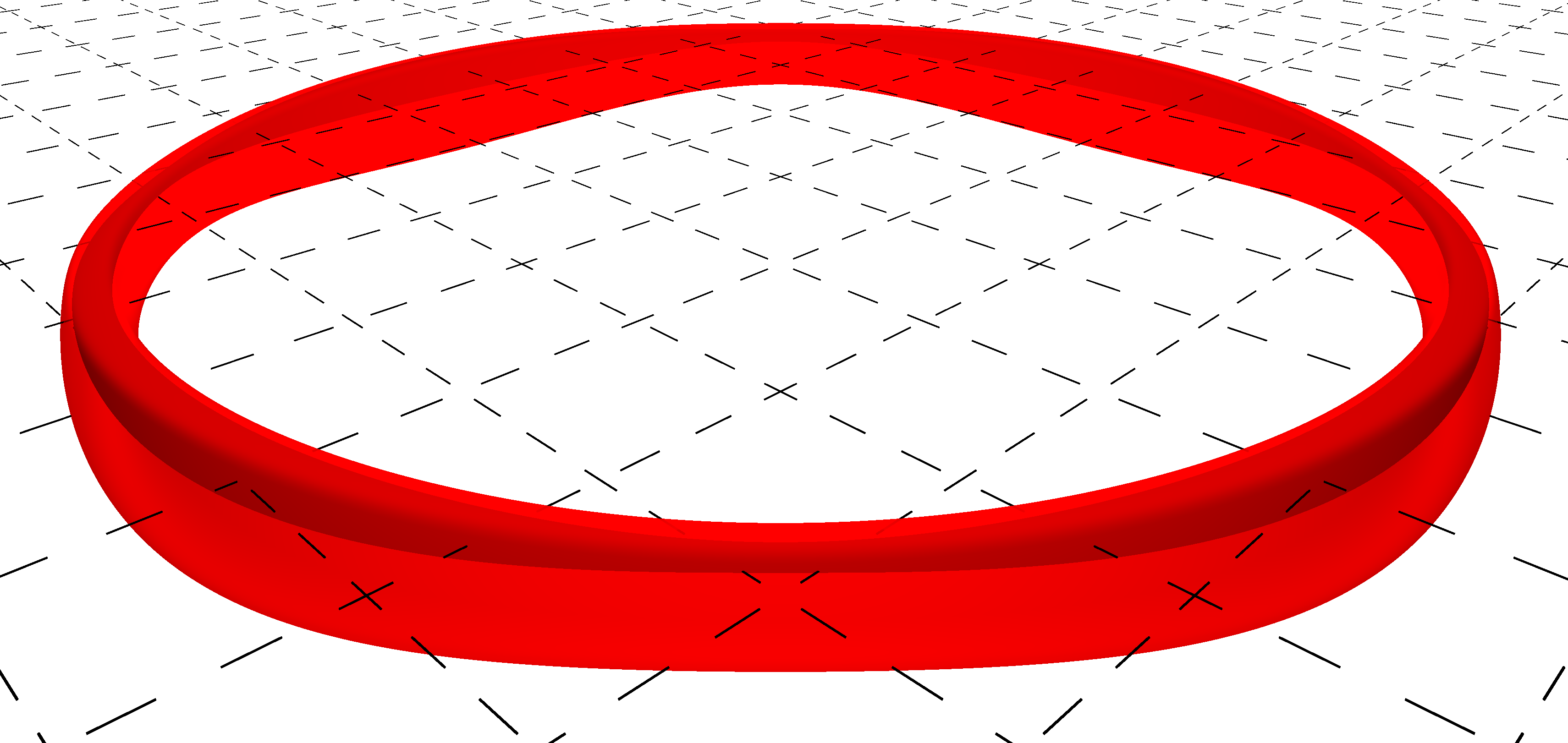
Figure 5: Isosurfaces for $E=0,-2~{}$\mathrm{meV}$$ (outer and inner surface, respectively) of the strain potential induced by a toroidal stressor pressed onto a Cu${}_{\text{2}}$O crystal along the $[001]$ axis with $\hat{\sigma}=-0.65$\mathrm{GPa}$$. The radius (center of torus to center of contact area) was set to $\rho=20b$, the grid lines are separated by $5b$.

IV Influence of strain on the binding energies of Rydberg excitons

As the excitonic states of interest in this study are odd-parity Rydberg states, the exchange interaction (which does not affect odd-parity states) and the coupling to the green exciton series via the kinetic Hamiltonian (4) (which should mostly affect states with large momentum space extension, i.e. small principal quantum number $n$) will be ignored. This enables the calculation of the excitonic binding energies by solving the anisotropic Wannier equation of a spinless two-band model

$$\left[T(\bm{k},\bm{\epsilon})+V_{e-h}(\bm{k})\star\right]\phi(\bm{k})=E\phi(\bm{k})$$ (18)

with the convolution operator of the momentum-space Coulomb potential Szmytkowski (2012); Schöne et al. (2016) $V_{e-h}(\bm{k})$

$$V_{e-h}(\bm{k})\star\phi(\bm{k})=\frac{1}{(2\pi)^{3/2}}\int d^{3}\bm{k}^{\prime}V_{e-h}(\bm{k}-\bm{k}^{\prime})\phi(\bm{k}^{\prime})$$ (19)

and one eigenvalue $T(\bm{k},\bm{\epsilon})$ of $\mathcal{H}_{r}(\bm{k},\bm{\epsilon})$ corresponding to a product state of a hole in a $\Gamma^{+}_{7}$ state with an electron in a $\Gamma^{+}_{6}$ state. The approach to the solution of Eq. (18) used in this study is discussed in Appendix A.

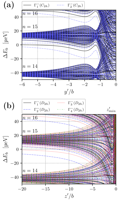
Figure 6: Binding-energy shifts $\Delta E_{b}$ of the odd-parity excitons with $n=14,15$ and $16$ relative to the strain-free $15P$ resonance ($E_{b}=-397~{}$\mathrm{\SIUnitSymbolMicro eV}$$) for $\hat{\sigma}=-0.65~{}$\mathrm{GPa}$$ and the geometry of Fig. 2 (a). The energies are sampled along lines through the potential minimum parallel to the $y^{\prime}$- and $z^{\prime}$-axis, respectively. (a): $z^{\prime}=z^{\prime}_{min}=-0.95\,b$, (b): $y^{\prime}=0$.
The colors and linestyles denote the irreducible representations of the respective states and are the same as in Fig. 7.

In what follows, we will assume that the coordinates of the stress field $x^{\prime}$, $y^{\prime}$ and $z^{\prime}$ coincide with the crystal axes $x$, $y$ and $z$ (see Fig. 2 (a)). At $y=0$, the strain becomes biaxial along $y$ and $z$ which reduces the local symmetry to $D_{2h}$ Bir and Pikus (1974). This does potentially lift all degeneracies in the spin-less two-band model as all irreducible representations of the single group are one-dimensional. For $y\neq 0$, the strain is still confined to the $(y,z)$-plane (i.e. $\epsilon_{xx}=\epsilon_{xy}=\epsilon_{zx}=0$), but the local symmetry reduces even further to $C_{2h}$. For other orientations of the stressor relative to the crystal axes, the local symmetries might be different. The only symmetry that is conserved under all (spatially homogeneous) strains is the inversion symmetry. Far from the contact zone $|y^{\prime}|\gg b\vee|z^{\prime}|\gg b$, the strain field vanishes and the $O_{h}$ symmetry is recovered.

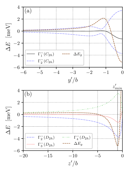
Figure 7: Binding-energy shifts $\Delta E_{b}$ of the $2P$ resonances relative to the strain-free case ($E_{b}=-24.57~{}$\mathrm{meV}$$) for the same conditions and with the same coding as in Fig. 6. The brown (dashed) line represents the band-gap shifts $\Delta E_{g}$ for comparison.

Figure 6 shows the binding energy shifts calculated from the two-band model including all odd-parity basis functions up to $\ell_{max}=25$ and $n_{max}=30+\ell$. The strain-induced shift in the binding energy $\Delta E_{b}$ is on the order of $\mathrm{\SIUnitSymbolMicro eV}$ for the Rydberg states. As the band-gap shift is on the order of $\mathrm{meV}$, it is the dominant potential contribution for states with large $n$: $\Delta E(\bm{r})\approx\Delta E_{g}(\bm{r})$. The energetical distance between adjacent states might become important if one tries to address specific states inside the trap. Due to finite laser spot-sizes, spectra will always contain a spatial average over the strain shifts in the region of the laser spot.

For states with lower $n$, $\Delta E_{b}$ might reach the same order of magnitude as $\Delta E_{g}$. This is shown in Fig. 7, which compares the shifts of the 2P resonances for the same conditions as in Fig. 6. In the region of the minimum of $\Delta E_{g}(\bm{r}_{min})=$-5.2\text{\,}\mathrm{meV}$$ , $\Delta E_{b}$ reaches values of $-3.7\text{\,}\mathrm{meV}$ for $\Gamma^{-}_{2}(D_{2h})$, $-1.3\text{\,}\mathrm{meV}$ for $\Gamma^{-}_{3}(D_{2h})$ and $3.4\text{\,}\mathrm{meV}$ for $\Gamma^{-}_{4}(D_{2h})$. The positions of the minima of the total potential $\Delta E_{b}+\Delta E_{g}$ differ slightly for the different symmetries, varying from $z^{\prime}=-0.94~{}b$ for $\Gamma^{-}_{2}(D_{2h})$ to $z^{\prime}=-1.0~{}b$ for $\Gamma^{-}_{4}(D_{2h})$.

V Conclusion and Outlook

We have shown that one can exploit the band-gap modification in a crystal to generate strain waveguides for Rydberg excitons that have similar or even superior parameters to optical dipole traps for atoms. For example, trap frequencies up to GHz and trap depths on the order of meV can potentially be reached. This implies that similar trapping geometries than those developed for atoms can be produced for excitons. The choice of stressor, together with the crystal orientation, determines the precise shape of the trapping potential with the possibility to create complex potential landscapes.

Our calculations have shown that, if one is only interested in the excitonic strain potential, it suffices to consider only the band-gap shift $\Delta E_{g}$ for the Rydberg states as it is about two orders of magnitude larger than the shift of the binding energies. The Rydberg states do, however, show a strong coupling, and potentially chaotic motion, in regions of high strain. Moreover, strain is known to influence the lifetime of excitons which will be the subject of future work.

Appendix A Numerical solution of the anisotropic two-band model

We will briefly review the numerical method used to compute the solutions of the isotropic, nonparabolic Wannier equation Schöne et al. (2016), and extend it to anisotropic band structures. Starting point is the anisotropic momentum-space Wannier equation (18) written as a Sturmian eigenvalue problem

$$\left[\frac{\hbar^{2}\bm{k}^{2}}{2\mu}+\Delta T(\bm{k})-E\right]\Psi(\bm{k})=-\lambda(E)~{}V_{e-h}(\bm{k})\star\Psi(\bm{k})$$ (20)

with the anisotropic, nonparabolic part of the hole dispersion $\Delta T(\bm{k})$ and the reduced effective electron-hole mass $\mu$, which both might depend on the strain tensor $\bm{\epsilon}$. In this calculation, however, the strain field is assumed to be constant over the extension of the exciton and those dependencies are not considered explicitly.

The Sturmian eigenvalues $\lambda(E)$ mark the excitonic eigenenergies $E_{n,\Gamma}$ by the condition $\lambda(E_{n,\Gamma})=1$. Hence, there is a parametric dependence of Eq. (20) on the sought energy eigenvalue $E$ which can be solved for the $\lambda(E)$ and the excitonic eigenenergies retrieved from them.

In contrast to Ref. Schöne et al. (2016), $\Delta T(\bm{k})$ is no longer assumed to be isotropic, but may transform according to $\Gamma^{+}_{1}$ of $O_{h}$ without strain and may retain only the inversion symmetry for arbitrary strain. In the strainless case, the exciton states split according to S$\mapsto\Gamma^{+}_{1}$, P$\mapsto\Gamma^{-}_{4}$, D$\mapsto\Gamma^{+}_{3}\oplus\Gamma^{+}_{5}$ and F$\mapsto\Gamma^{-}_{2}\oplus\Gamma^{-}_{4}\oplus\Gamma^{-}_{5}$ in this model Koster et al. (1963). Therefore, trial functions with the correct symmetries can be constructed as

$$\Psi_{\Gamma_{j}}(\bm{k})=\sum_{\ell_{\alpha}}~{}F^{\Gamma_{j}}_{\ell_{\alpha}}(k)~{}\psi^{\Gamma_{j}}_{\ell_{\alpha}}(\bm{n}_{k}),$$ (21)

where $\psi^{\Gamma_{j}}_{\ell_{\alpha}}(\bm{n}_{k})$ is the $\alpha$th cubic harmonic Von der Lage and Bethe (1947) of order $\ell$ that transforms like a basis function $\Gamma_{j}$ of the irreducible representation $\Gamma$, and $F^{\Gamma_{j}}_{\ell_{\alpha}}(k)$ is the corresponding radial wave function. In terms of the spherical harmonics $Y_{\ell}^{m}(\bm{n}_{k})$, the relevant real-valued cubic harmonics up to fifth order for $\Gamma^{-}_{4,z}$ and tenth order for $\Gamma^{+}_{1}$ are

$$\psi^{\Gamma^{+}_{1}}_{0_{1}}=Y_{0}^{0},$$ (22)

$$\psi^{\Gamma^{+}_{1}}_{4_{1}}=\sqrt{\frac{5}{24}}(Y^{4}_{4}+Y^{-4}_{4})+\sqrt{\frac{7}{12}}Y^{0}_{4},$$ (23)

$$\psi^{\Gamma^{+}_{1}}_{6_{1}}=\sqrt{\frac{7}{16}}(Y^{4}_{6}+Y^{-4}_{6})-\sqrt{\frac{1}{8}}Y^{0}_{6},$$ (24)

$$\psi^{\Gamma^{+}_{1}}_{8_{1}}=\sqrt{\frac{65}{384}}(Y^{8}_{8}+Y^{-8}_{8})+\sqrt{\frac{7}{96}}(Y^{4}_{8}+Y^{-4}_{8})$$

$$+\sqrt{\frac{33}{64}}Y^{0}_{8},$$ (25)

$$\psi^{\Gamma^{+}_{1}}_{10_{1}}=\sqrt{\frac{187}{768}}(Y^{8}_{10}+Y^{-8}_{10})+\sqrt{\frac{11}{64}}(Y^{4}_{10}+Y^{-4}_{10})$$

$$-\sqrt{\frac{65}{384}}Y^{0}_{10},$$ (26)

$$\psi^{\Gamma^{-}_{4,z}}_{1_{1}}=Y^{0}_{1},$$ (27)

$$\psi^{\Gamma^{-}_{4,z}}_{3_{1}}=Y^{0}_{3},$$ (28)

$$\psi^{\Gamma^{-}_{4,z}}_{5_{1}}=Y^{0}_{5},$$ (29)

$$\psi^{\Gamma^{-}_{4,z}}_{5_{2}}=\sqrt{\frac{1}{2}}(Y^{4}_{5}+Y^{-4}_{5}).$$ (30)

Inserting the expansion into Eq. (20) while simultaneously expanding

$$D(\bm{k}):=\frac{2\mu\Delta T(\bm{k})}{\hbar^{2}}=\sum_{\ell_{\alpha}^{\prime\prime}}~{}D_{\ell_{\alpha}^{\prime\prime}}(k)~{}\psi^{\Gamma^{+}_{1}}_{\ell_{\alpha}^{\prime\prime}}(\bm{n}_{k}),$$ (31)

yields

$$\sum\limits_{\ell_{\alpha}^{\prime}}\left[\left(k^{2}+q^{2}\right)\delta_{\ell_{\alpha},\ell_{\alpha}^{\prime}}+\sum\limits_{\ell_{\alpha}^{\prime\prime}}~{}D_{\ell_{\alpha}^{\prime\prime}}(k)~{}C^{\Gamma_{j}}_{\ell_{\alpha},\ell_{\alpha}^{\prime},\ell_{\alpha}^{\prime\prime}}\right]F^{\Gamma_{j}}_{\ell_{\alpha}^{\prime}}(k)$$

$$=\frac{2\lambda(q)}{\pi a_{B}k}~{}\int\limits_{0}^{\infty}dk^{\prime}~{}k^{\prime}~{}F^{\Gamma_{j}}_{\ell_{\alpha}}(k^{\prime})~{}Q_{\ell}\left(\frac{k^{2}+k^{\prime 2}}{2kk^{\prime}}\right)$$ (32)

after multiplication by $\psi^{\Gamma_{j}\dagger}_{\ell_{\alpha}}(\bm{n}_{k})$ and integration over the unit sphere (for details, see Ref. Szmytkowski (2012)). Here, $Q_{\ell}(x)$ denotes the Legendre functions of the second kind, $q=\sqrt{2\mu|E|}/\hbar$ is the renormalised energy, $a_{B}=4\pi\varepsilon_{0}\varepsilon_{r}\hbar^{2}/(\mu e^{2})$ the excitonic Bohr radius and

$$C^{\Gamma_{j}}_{\ell_{\alpha},\ell_{\alpha}^{\prime},\ell_{\alpha}^{\prime\prime}}=\oint d^{2}\bm{n}_{k}~{}\psi^{\Gamma_{j}\dagger}_{\ell_{\alpha}}(\bm{n}_{k})~{}\psi^{\Gamma^{+}_{1}}_{\ell_{\alpha}^{\prime\prime}}(\bm{n}_{k})~{}\psi^{\Gamma_{j}}_{\ell_{\alpha}^{\prime}}(\bm{n}_{k})$$ (33)

the coupling coefficients of the cubic harmonics, which can be evaluated in terms of Wigner 3-j symbols. Equation (32) can be rewritten as

$$J^{\Gamma_{j}}_{\ell_{\alpha}}(k)=\frac{2\lambda(q)}{\pi a_{B}}\sum\limits_{\ell_{\alpha}^{\prime}}\int\limits_{0}^{\infty}dk^{\prime}~{}\left[\bm{T}^{-1}_{\Gamma_{j}}(k^{\prime},q)\right]_{\ell_{\alpha},\ell_{\alpha}^{\prime}}J^{\Gamma_{j}}_{\ell_{\alpha}^{\prime}}(k^{\prime})$$

$$\times\frac{Q_{\ell}\left(\frac{k^{2}+k^{\prime 2}}{2kk^{\prime}}\right)}{\sqrt{k^{2}+q^{2}}\sqrt{k^{\prime 2}+q^{2}}}$$ (34)

where

$$J^{\Gamma_{j}}_{\ell_{\alpha}}(k)=k\sqrt{k^{2}+q^{2}}\sum_{\ell_{\alpha}^{\prime}}\left[\bm{T}_{\Gamma_{j}}(k,q)\right]_{\ell_{\alpha},\ell_{\alpha}^{\prime}}F^{\Gamma_{j}}_{\ell_{\alpha}^{\prime}}(k)$$ (35)

and

$$\left[\bm{T}_{\Gamma_{j}}(k,q)\right]_{\ell_{\alpha},\ell_{\alpha}^{\prime}}=\delta_{\ell_{\alpha},\ell_{\alpha}^{\prime}}+\sum\limits_{\ell_{\alpha}^{\prime\prime}}~{}\frac{D_{\ell_{\alpha}^{\prime\prime}}(k)}{k^{2}+q^{2}}C^{\Gamma_{j}}_{\ell_{\alpha},\ell_{\alpha}^{\prime},\ell_{\alpha}^{\prime\prime}}.$$ (36)

As in the case of an isotropic band structure, the $k$-dependent part of the integral kernel in Eq. (34) can be expressed as Szmytkowski (2012)

$$M_{\ell}(q,k,k^{\prime})=\frac{2}{\pi a_{B}}~{}\frac{Q_{\ell}\left(\frac{k^{2}+k^{\prime 2}}{2kk^{\prime}}\right)}{\sqrt{k^{2}+q^{2}}\sqrt{k^{\prime 2}+q^{2}}}$$

$$=\sum\limits_{n_{r}=0}^{\infty}g_{n_{r},\ell}(k,q)~{}g_{n_{r},\ell}(k^{\prime},q)$$ (37)

where

$$g_{n_{r},\ell}(k,q)=\ell!\sqrt{\frac{n_{r}!}{\pi~{}a_{B}~{}(n_{r}+2\ell+1)!}}\frac{(4qk)^{\ell+1}}{(q^{2}+k^{2})^{\ell+3/2}}$$

$$\times C^{(\ell+1)}_{n_{r}}\left(\frac{q^{2}-k^{2}}{q^{2}+k^{2}}\right)$$ (38)

with the Gegenbauer polynomials $C^{(\alpha)}_{n_{r}}(x)$. The functions $g_{n_{r},\ell}(k,q)$ are orthogonal with respect to the radial quantum number $n_{r}$,

$$\int\limits_{0}^{\infty}dk~{}g_{n_{r},\ell}(k,q)g_{n_{r}^{\prime},\ell}(k,q)=\delta_{n_{r},n_{r}^{\prime}}\frac{1}{q~{}a_{B}~{}(n_{r}+\ell+1)},$$ (39)

and they form a natural basis in which to expand the $J^{\Gamma_{j}}_{\ell_{\alpha}}(k)$ in order to solve Eq. (34) numerically.

In the case of strain, the calculation is equivalent with the exception that the correct lattice harmonics have to be chosen as the angular expansion functions (e. g. those for the point groups $C_{2h}$ and $D_{2h}$ for the $y^{\prime}$- and $z^{\prime}$-directions in Sec. IV or $C_{i}$ in the most general case). These can be constructed by comparing the coupling coefficients given by Koster Koster et al. (1963) and the Clebsch-Gordan coefficients.

For $D_{2h}$, the odd-parity lattice harmonics are (with odd $\ell$ and the obvious limits on $\alpha$)

$$\psi^{\Gamma^{-}_{1}}_{\ell_{\alpha}}=i\sqrt{\frac{1}{2}}\left(Y_{\ell}^{2\alpha}-Y_{\ell}^{-2\alpha}\right),$$ (40)

$$\psi^{\Gamma^{-}_{2}}_{\ell_{\alpha}}=i\sqrt{\frac{1}{2}}\left(Y_{\ell}^{2\alpha+1}+Y_{\ell}^{-(2\alpha+1)}\right),$$ (41)

$$\psi^{\Gamma^{-}_{3}}_{\ell_{0}}=Y_{\ell}^{0},$$ (42)

$$\psi^{\Gamma^{-}_{3}}_{\ell_{\alpha}}=\sqrt{\frac{1}{2}}\left(Y_{\ell}^{2\alpha}+Y_{\ell}^{-2\alpha}\right),$$ (43)

$$\psi^{\Gamma^{-}_{4}}_{\ell_{\alpha}}=\sqrt{\frac{1}{2}}\left(Y_{\ell}^{2\alpha+1}-Y_{\ell}^{-(2\alpha+1)}\right).$$ (44)

For $C_{2h}$ they can be expressed as

$$\psi^{\Gamma^{-}_{1}}_{\ell_{\alpha_{\pm}}}=\sqrt{\pm\frac{1}{2}}\left(Y_{\ell}^{2\alpha}\pm Y_{\ell}^{-2\alpha}\right),$$ (45)

$$\psi^{\Gamma^{-}_{1}}_{\ell_{0}}=Y_{\ell}^{0},$$ (46)

$$\psi^{\Gamma^{-}_{2}}_{\ell_{\alpha_{\pm}}}=\sqrt{\mp\frac{1}{2}}\left(Y_{\ell}^{2\alpha+1}\pm Y_{\ell}^{-(2\alpha+1)}\right),$$ (47)

if the $z$-axis is chosen as the twofold rotation axis. For $C_{i}$ every odd-parity function belongs to $\Gamma^{-}_{1}$.

The $\bm{k}$-space extension of the Rydberg states scales roughly as $n^{-1}$. Therefore, the most important terms for highly excited states in (31) are those with $D_{l_{\alpha}}(k)\propto k^{2}$ for $k\rightarrow 0$, which is only fulfilled by terms of zeroth and second order for the $\Gamma^{+}_{7}$ band. Including only those quadratic terms, the problem at hand can be expressed as the anisotropic Kepler problem

$$\left[\frac{\hbar^{2}k_{x}^{2}}{2m_{x}}+\frac{\hbar^{2}k_{y}^{2}}{2m_{y}}+\frac{\hbar^{2}k_{z}^{2}}{2m_{z}}+V_{e-h}(\bm{k})\star\right]\phi(\bm{k})=E\phi(\bm{k}).$$ (48)

For $O_{h}$-symmetry, there are no terms with $\ell=2$ that transform like $\Gamma^{+}_{1}$, and the effective mass at the zone center of the $\Gamma^{+}_{7}$ valence band is isotropic. Hence, the coupling between different $\ell$ is small and the ansatz (21) can be truncated at low $\ell_{\alpha}$. Inside the traps, the effective mass is quite anisotropic and states of different $\ell$ couple strongly. Therefore, all odd-parity basis functions with $n_{r}=n-\ell-1\leq 29$ and $\ell\leq 25$ had to be included, in order for the calculation of the binding-energy shifts of the $n=15$ resonances to converge (giving bases of up to $\sim 5500$ basis functions). As the number of basis states scales with $n^{2}$, the algorithm becomes computationally very expensive and not feasible for $n\gtrsim 15$.

References

Gross and Karryev (1952)E. F. Gross and N. A. Karryev, Doklady Akademii Nauk SSSR 84, 471 (1952).
Gross (1956)E. F. Gross, Il
Nuovo Cimento (1955-1965) 3, 672 (1956).
Kazimierczuk et al. (2014)T. Kazimierczuk, D. Fröhlich, S. Scheel, H. Stolz, and M. Bayer, Nature 514, 343 (2014).
Thewes et al. (2015)J. Thewes, J. Heckötter, T. Kazimierczuk, M. Aßmann, D. Fröhlich, M. Bayer,
M. A. Semina, and M. M. Glazov, Physical review
letters 115, 027402
(2015).
Schöne et al. (2016)F. Schöne, S.-O. Krüger, P. Grünwald, H. Stolz,
S. Scheel, M. Aßmann, J. Heckötter, J. Thewes, D. Fröhlich, and M. Bayer, Physical Review B 93, 075203 (2016).
Grünwald et al. (2016)P. Grünwald, M. Aßmann, J. Heckötter, D. Fröhlich, M. Bayer,
H. Stolz, and S. Scheel, Physical review letters 117, 133003 (2016).
Trauernicht et al. (1986)D. P. Trauernicht, J. P. Wolfe, and A. Mysyrowicz, Physical Review B 34, 2561 (1986).
Snoke and Negoita (2000)D. W. Snoke and V. Negoita, Physical Review B 61, 2904 (2000).
Naka and Nagasawa (2002)N. Naka and N. Nagasawa, Physical Review B 65, 075209 (2002).
Naka and Nagasawa (2004)N. Naka and N. Nagasawa, Physical Review B 70, 155205 (2004).
Yoshioka et al. (2011)K. Yoshioka, E. Chae, and M. Kuwata-Gonokami, Nature
communications 2, 328
(2011).
Stolz et al. (2012)H. Stolz, R. Schwartz,
F. Kieseling, S. Som, M. Kaupsch, S. Sobkowiak, D. Semkat, N. Naka, T. Koch, and H. Fehske, New
Journal of physics 14, 105007 (2012).
Schwartz et al. (2012)R. Schwartz, N. Naka,
F. Kieseling, and H. Stolz, New Journal of Physics 14, 023054 (2012).
Iwamitsu et al. (2014)K. Iwamitsu, S. Aihara,
A. Ota, F. Ichikawa, T. Shimamoto, and I. Akai, Journal of the Physical Society of Japan 83, 124714 (2014).
Sandfort et al. (2011)C. Sandfort, J. Brandt,
C. Finke, D. Fröhlich, M. Bayer, H. Stolz, and N. Naka, Physical Review B 84, 165215 (2011).
Grimm et al. (2000)R. Grimm, M. Weidemüller, and Y. B. Ovchinnikov, Advances in atomic, molecular, and optical physics 42, 95 (2000).
Markiewicz et al. (1977)R. S. Markiewicz, J. P. Wolfe, and C. D. Jeffries, Physical Review B 15, 1988 (1977).
Note (1)The original paper apparently contains a sign error in the
definition of as the equations given there do not describe a
plane strain, as claimed ( for isotropic
materials).
Schweiner et al. (2016)F. Schweiner, J. Main, and G. Wunner, Physical Review
B 93, 085203 (2016).
Denev and Snoke (2002)S. Denev and D. W. Snoke, Physical Review B 65, 085211 (2002).
Szmytkowski (2012)R. Szmytkowski, Annalen der Physik 524, 345 (2012).
Bir and Pikus (1974)G. L. Bir and G. E. Pikus, Symmetry and
strain-induced effects in semiconductors, Vol. 624 (Wiley New York, 1974).
Koster et al. (1963)G. F. Koster, J. O. Dimmock,
R. G. Wheeler, and H. Statz, Properties of the 32-point
groups (1963).
Von der Lage and Bethe (1947)F. C. Von der Lage and H. A. Bethe, Physical Review 71, 612
(1947).