CERN-TH-2017-232

ZU-TH 30/17

Fully differential NNLO computations with MATRIX

Massimiliano Grazzini^(a), Stefan Kallweit^(b) and Marius Wiesemann^(b)

^(a)Physik-Institut, Universität Zürich, CH-8057 Zürich, Switzerland

^(b)TH Division, Physics Department, CERN, CH-1211 Geneva 23, Switzerland

grazzini@physik.uzh.ch
stefan.kallweit@cern.ch
marius.wiesemann@cern.ch

Abstract

We present the computational framework Matrix [1] which allows us to evaluate fully differential cross sections for a wide class of processes at hadron colliders in next-to-next-to-leading order (NNLO) QCD. The processes we consider are $2\to 1$ and $2\to 2$ hadronic reactions involving Higgs and vector bosons in the final state. All possible leptonic decay channels of the vector bosons are included for the first time in the calculations, by consistently accounting for all resonant and non-resonant diagrams, off-shell effects and spin correlations. We briefly introduce the theoretical framework Matrix is based on, discuss its relevant features and provide a detailed description of how to use Matrix to obtain NNLO accurate results for the various processes. We report reference predictions for inclusive and fiducial cross sections of all the physics processes considered here and discuss their corresponding uncertainties. Matrix features an automatic extrapolation procedure that allows us, for the first time, to control the systematic uncertainties inherent to the applied NNLO subtraction procedure down to the few permille level (or better).

November 2017

1 Introduction

Precision computations for Standard Model (SM) processes are vital for the rich physics programme at the LHC. The increasing amount of collected data pushes the experimental uncertainties down to the percent level, thereby demanding accurate predictions for many relevant physics processes. This holds not only for SM measurements. Also new-physics searches rely on a precise modelling of the SM backgrounds. In particular, the sensitivity to small deviations from the SM predictions directly depends on the size of theoretical uncertainties. Besides single vector-boson and Higgs boson production processes, vector-boson pair production is particularly important in that respect since anomalous triple gauge couplings would be first uncovered in cross sections and distributions of the diboson processes.

Precise SM computations require, in particular, the inclusion of QCD radiative corrections at the next-to-leading order (NLO), and if possible at the next-to-next-to-leading order (NNLO). NNLO QCD predictions for the simplest hadronic reactions have been available for quite some time. The pioneering computation of the inclusive cross section for vector-boson production was carried out in the ’90s [2]. The corresponding computation for Higgs boson production was performed about ten years later [3, 4, 5]. They were followed by the calculation of the rapidity distribution of vector bosons [6]. Shortly after, fully differential calculations for Higgs and vector-boson production started to appear [7, 8, 9, 10, 11, 12]. This further step was essential to obtain realistic predictions since fully differential computations allow us to apply selection cuts on the produced boson and on its decay products, and to directly address all the relevant kinematic distributions. The last decade has seen a revolution in the field of NNLO computations: The calculations for associated production of a Higgs boson with a vector boson [13, 14, 15, 16], Higgs boson production in bottom-quark annihilation [17, 18, 19, 20], top-mass effects in Higgs boson production [21, 22, 23, 24, 25], $HH$ [26, 27], $\gamma\gamma$ [28, 29], $Z\gamma$ [30, 31, 32], $W\gamma$ [31], $ZZ$ [33, 34, 35], $W^{+}W^{-}$ [36, 37] and $W^{\pm}Z$ [38, 39] production have been completed. NNLO results have been achieved also for further important processes like top-quark pair [40, 41] and single top [42] production, dijet production [43], Higgs production through vector-boson fusion [44], $H$+jet [45, 46, 47], $\gamma$+jet [48], $Z$+jet [49, 50] and $W$+jet [51]. Despite this tremendous progress, at present, publicly available NNLO programs typically carry out fully differential NNLO computations for a limited set of specific processes. Examples are FEWZ [52] and DYNNLO [12] for vector-boson production, FehiPro [7, 53] and HNNLO [9, 11] for Higgs boson production, and 2$\gamma$NNLO [28] for diphoton production. A notable exception is MCFM [54], which in its current release features an NNLO implementation of single vector-boson and Higgs boson production, associated production of a Higgs boson with a vector-boson, and diphoton production.

In this paper, we present the computational framework Matrix, which features a parton-level Monte Carlo generator capable of computing fiducial cross sections and distributions for Higgs boson, vector-boson and vector-boson pair production processes up to NNLO in QCD. For the first time, we consider all possible leptonic decay channels of the vector bosons, and we include spin correlations and off-shell effects by accounting for all resonant and non-resonant diagrams, thereby allowing the user to apply realistic fiducial cuts directly on the phase-space of the respective leptonic final state. Matrix achieves NNLO accuracy by using a process-independent implementation of the $q_{T}$-subtraction formalism [9] in combination with a fully automated implementation of the Catani–Seymour dipole subtraction method [55, 56] within the Monte Carlo program Munich. All (spin- and colour-correlated) tree-level and one-loop amplitudes are obtained from OpenLoops [57, 58]. Early versions of Matrix have been used, in combination with the two-loop scattering amplitudes of Refs. [59, 60, 61], for the NNLO calculations of $Z\gamma$ [30, 31], $W^{\pm}\gamma$ [31] $ZZ$ [33, 34], $W^{+}W^{-}$ [36, 37], $W^{\pm}Z$ [38, 39] and $HH$ [27] production and the importance of including NNLO corrections for these processes is evident for both total rates and differential distributions. Matrix provides a fully automated extrapolation procedure that allows us, for the first time, to control the systematic uncertainties inherent to the $q_{T}$-subtraction procedure down to the few permille level (or better) for all NNLO predictions. The Matrix framework offers a simple interface to a powerful code to carry out such computations in a relatively straightforward way, and its first public version is now available for download [1].

The manuscript is organized as follows: In Section 2 we give a general introduction into the Matrix framework, where we review the $q_{T}$-subtraction formalism and describe the organization of the computations. We then provide detailed instructions on how to use the code: This involves the generation, compilation and running of a process to compute LO, NLO and NNLO cross sections in Section 3, and a detailed description of the relevant input files and parameters in Section 4. In Section 5 we provide benchmark predictions for total and fiducial rates, respectively, for all processes, including the results of our novel extrapolation procedure, and we discuss the relevant physics features of each process. A discussion of the systematic uncertainties of NNLO cross sections computed with $q_{T}$ subtraction for a representative set of processes and details on the extrapolation procedure are presented in Section 6. In Section 7 we summarize our results. All predefined phase-space cuts are listed in Appendix A. How to extend the predefined set of cuts, distributions and dynamic scales by modifying the underlying C++ code is sketched in Appendix B. Finally, Appendix C provides a loose selection of solutions on compilation and running issues, which have been encountered in the testing phase of Matrix and are expected to be potentially helpful for the user.

2 NNLO computations in the MATRIX framework

The computation of a QCD cross section at NNLO requires the evaluation of tree-level contributions with up to two additional unresolved partons, of one-loop contributions with one unresolved parton and of purely virtual contributions. The implementation of the corresponding scattering amplitudes in a complete NNLO calculation at the fully differential (exclusive) level is a highly non-trivial task because of the presence of infrared (IR) divergences at intermediate stages of the calculation. In particular, since the divergences affect real and virtual contributions in a different way, a straightforward combination of these components is not possible. Various methods have been proposed and used to overcome these issues at NNLO [63, 64, 65, 66, 9, 67, 68, 69, 70, 71, 72, 51, 73, 74, 75]. The method applied by Matrix is transverse-momentum ($q_{T}$) subtraction [9], and it is briefly described below.

2.1 The $\boldsymbol{q_{T}}$-subtraction formalism

The $q_{T}$-subtraction formalism [9] is a method to handle and cancel IR divergences at NLO and NNLO. The method exploits the fact that for the production of a colourless final-state system (i.e. a system composed of particles without QCD interactions) the behaviour of the $q_{T}$ distribution at small $q_{T}$ has a universal (process-independent) structure that is explicitly known up to NNLO through the formalism of transverse-momentum resummation [76, 77]. This knowledge is sufficient to fully determine the $q_{T}$ dependence of the cross section at small $q_{T}$ and to construct a non-local, but process-independent IR subtraction counterterm for this entire class of processes.

In the $q_{T}$-subtraction method, the cross section for a generic process $pp\to F+X$, where $F$ is a colourless system as specified above, can be written up to (N)NLO as

$${\rm d}{\sigma}^{\mathrm{F}}_{\mathrm{(N)NLO}}={\cal H}^{\mathrm{F}}_{\mathrm{(N)NLO}}\otimes{\rm d}{\sigma}^{\mathrm{F}}_{\mathrm{LO}}+\left[{\rm d}{\sigma}^{\mathrm{F+jet}}_{\mathrm{(N)LO}}-{\rm d}{\sigma}^{\mathrm{CT}}_{\mathrm{(N)NLO}}\right].$$ (1)

The term $d{\sigma}^{\mathrm{F+jet}}_{\mathrm{(N)LO}}$ represents the cross section for the production of the system $F+$jet at (N)LO accuracy. If Eq. (1) is applied at NLO, the LO cross section $d{\sigma}^{\mathrm{F+jet}}_{\mathrm{LO}}$ can be obtained by direct integration of the corresponding tree-level amplitudes. If Eq. (1) is applied at NNLO, the NLO cross section $d{\sigma}^{\mathrm{F+jet}}_{\mathrm{NLO}}$ can be evaluated by using any available NLO subtraction method [79, 80, 55, 56] to handle and cancel the corresponding IR divergencies. Therefore, $d{\sigma}^{\mathrm{F+jet}}_{\mathrm{NLO}}$ is finite provided that $q_{T}\neq 0$, but it diverges in the limit $q_{T}\to 0$. The process-independent counterterm $\mathrm{d}{\sigma}^{\mathrm{CT}}_{\mathrm{(N)NLO}}$ guarantees the cancellation of this divergence of the $F+$jet cross section, and its general expression is provided in Ref. [77]. The numerical implementation of the contribution in the square bracket in Eq. (1), which is by construction finite in the limit $q_{T}\to 0$, is discussed in detail in Section 2.2. The computation is completed by evaluating the first term on the right-hand side of Eq. (1), which depends on the hard-collinear coefficients ${\cal H}^{\mathrm{F}}_{\mathrm{NLO}}$ and ${\cal H}^{\mathrm{F}}_{\mathrm{NNLO}}$, respectively, at NLO and NNLO. The structure of the NLO coefficient ${\cal H}^{\mathrm{F}}_{\mathrm{NLO}}$ has been obtained in a universal way from the one-loop corrections to the respective Born subprocess [81]. The general form of ${\cal H}^{\mathrm{F}}_{\mathrm{NNLO}}$ is also known [82]: It has been derived from the explicit results for Higgs [83] and vector-boson [84] production in terms of the suitably subtracted two-loop corrections to the respective Born subprocesses. Thus, if the $q{\bar{q}}\to F$ (or $gg\to F$) two-loop amplitude is available, the coefficient ${\cal H}^{\mathrm{F}}_{\mathrm{NNLO}}$ can be straightforwardly extracted.

2.2 Implementation within the MATRIX framework

Matrix provides a process library for the computation of colour-singlet processes at NNLO QCD. The core of the Matrix framework is the Monte Carlo program Munich, which is capable of computing both QCD and EW [85, 86] corrections to any SM process at NLO accuracy. Munich employs an automated implementation of the Catani–Seymour dipole-subtraction method for massless [55, 56] and massive [87] partons, and contains a general implementation of a very efficient, multi-channel based phase-space integration. All amplitudes up to one-loop level are supplied by OpenLoops [57] through an automated interface. With this functionality inherited from Munich, Matrix is immediately able to perform in principle any SM calculation up to NLO accuracy. To promote Munich to a Monte Carlo integrator at NNLO QCD, the $F+$jet cross section at NLO ($d{\sigma}^{\mathrm{F+jet}}_{\mathrm{NLO}}$) is combined with a process-independent implementation of the $q_{T}$-subtraction formalism for both $gg$- and $q{\bar{q}}$-initiated processes within the Matrix framework. The universal nature of the counterterm $\mathrm{d}{\sigma}^{\mathrm{CT}}_{\mathrm{NNLO}}$ and the hard-collinear coefficients ${\cal H}^{\mathrm{F}}_{\mathrm{NNLO}}$ in Eq. (1) allows us to perform NNLO QCD computations for the hadroproduction of an arbitrary set of colourless final-state particles, provided that the corresponding two-loop virtual amplitudes to the Born-level subprocesses are available.

To this end, Matrix includes the hard-collinear coefficients of Ref. [83, 84], relevant for single Higgs and vector-boson production, and employs own implementations of the two-loop amplitudes for the associated production of a $W/Z$ boson with a photon [59] and $\gamma\gamma$ [93] production, whereas external codes are used for on-shell $ZZ$ [33] and $W^{+}W^{-}$ [36] production. The two-loop amplitudes for off-shell production of massive vector-boson pairs[60] are taken from the publicly available code VVamp [94]. Any new production process of colour singlets can be supplemented to the Matrix library upon implementation of the corresponding two-loop amplitudes, since all remaining process-dependent ingredients are available in Munich+OpenLoops and the implementation of the $q_{T}$-subtraction formalism is fully general.

While the idea behind the $q_{T}$-subtraction formalism has been outlined in the previous Section, one point deserves some additional discussion. The contribution in the square bracket in Eq. (1) is formally finite in the limit $q_{T}\to 0$, but both $\mathrm{d}{\sigma}^{\mathrm{F+jet}}_{\mathrm{(N)LO}}$ and $\mathrm{d}{\sigma}^{\mathrm{CT}}_{\mathrm{(N)NLO}}$ are separately divergent. Since the subtraction is non-local, we introduce a technical cut-off $r_{\mathrm{cut}}$ on the dimensionless quantity $r=q_{T}/M$ ($M$ being the invariant mass of the colourless system) which renders both terms separately finite. Below this cut-off, $\mathrm{d}{\sigma}^{\mathrm{F+jet}}_{\mathrm{(N)LO}}$ and $\mathrm{d}{\sigma}^{\mathrm{CT}}_{\mathrm{(N)NLO}}$ are assumed to be identical, which is correct up to power-suppressed contributions. The latter vanish in the limit $r_{\mathrm{cut}}\to 0$ and can be controlled by monitoring the $r_{\mathrm{cut}}$ dependence of the cross section. The absence of any residual logarithmic dependence on $r_{\mathrm{cut}}$ thus provides strong evidence of the correctness of the computation since any mismatch between the contributions would result in a divergence of the cross section for $r_{\mathrm{cut}}\to 0$. The cut-off on $r$ acts as a slicing parameter, and, correspondingly, the $q_{T}$-subtraction method as implemented in Matrix works very similar to a phase-space slicing method.

To monitor the $r_{\mathrm{cut}}$ dependence without the need of repeated CPU-intensive runs, Matrix simultaneously computes the cross section at several $r_{\mathrm{cut}}$ values. The numerical information on the $r_{\mathrm{cut}}$ dependence is used to address the limit $r_{\mathrm{cut}}\to 0$ by using a fit based on the results at finite $r_{\mathrm{cut}}$ values. The extrapolated result, including an estimate of the uncertainty of the extrapolation procedure, is provided at the end of each run. Details on the $r_{\mathrm{cut}}{}\rightarrow 0$ extrapolation and its uncertainty estimate are presented in Section 6, where we also discuss the $r_{\mathrm{cut}}$ dependence of a representative set of the processes available in the first release of Matrix.

3 How to use MATRIX

The code is engineered in a way that guides the user from the very first execution of Matrix to the very end of a run of a specific process, obtaining all relevant results. In-between there are certain steps/decisions to make (such as choosing the process, inputs, parameters, …), which will be described in more detail throughout this and the next Section.

The only thing we require the user of Matrix to provide on the machine where the code is executed is a working installation of LHAPDF, which is a well-known standard code by now, such that lhapdf-config is recognized as a terminal command, or that the path to the lhapdf-config executable is specified in the file MATRIX_configuration (see Section 3.5 for more details on the configuration of Matrix).

${process_id}		process		description
pph21		$pp/p\bar{p}\to H$		on-shell Higgs-boson production
ppz01		$pp/p\bar{p}\to Z$		on-shell $Z$ production
ppw01		$pp/p\bar{p}\to W^{-}$		on-shell $W^{-}$ production with CKM
ppwx01		$pp/p\bar{p}\to W^{+}$		on-shell $W^{+}$ production with CKM
ppeex02		$pp/p\bar{p}\to e^{-}e^{+}$		$Z$ production with decay
ppnenex02		$pp/p\bar{p}\to\nu_{e}\bar{\nu}_{e}$		$Z$ production with decay
ppenex02		$pp/p\bar{p}\to e^{-}\bar{\nu}_{e}$		$W^{-}$ production with decay and CKM
ppexne02		$pp/p\bar{p}\to e^{+}\nu_{e}$		$W^{+}$ production with decay and CKM
ppaa02		$pp/p\bar{p}\to\gamma\gamma$		$\gamma\gamma$ production
ppeexa03		$pp/p\bar{p}\to e^{-}e^{+}\gamma$		$Z\gamma$ production with decay
ppnenexa03		$pp/p\bar{p}\to\nu_{e}\bar{\nu}_{e}\gamma$		$Z\gamma$ production with decay
ppenexa03		$pp/p\bar{p}\to e^{-}\bar{\nu}_{e}\gamma$		$W^{-}\gamma$ with decay
ppexnea03		$pp/p\bar{p}\to e^{+}\nu_{e}\gamma$		$W^{+}\gamma$ with decay
ppzz02		$pp/p\bar{p}\to ZZ$		on-shell $ZZ$ production
ppwxw02		$pp/p\bar{p}\to W^{+}W^{-}$		on-shell $W^{+}W^{-}$ production
ppemexmx04		$pp/p\bar{p}\to e^{-}\mu^{-}e^{+}\mu^{+}$		$ZZ$ production with decay
ppeeexex04		$pp/p\bar{p}\to e^{-}e^{-}e^{+}e^{+}$		$ZZ$ production with decay
ppeexnmnmx04		$pp/p\bar{p}\to e^{-}e^{+}\nu_{\mu}\bar{\nu}_{\mu}$		$ZZ$ production with decay
ppemxnmnex04		$pp/p\bar{p}\to e^{-}\mu^{+}\nu_{\mu}\bar{\nu}_{e}$		$W^{+}W^{-}$ production with decay
ppeexnenex04		$pp/p\bar{p}\to e^{-}e^{+}\nu_{e}\bar{\nu}_{e}$		$ZZ$ / $W^{+}W^{-}$ production with decay
ppemexnmx04		$pp/p\bar{p}\to e^{-}\mu^{-}e^{+}\bar{\nu}_{\mu}$		$W^{-}Z$ production with decay
ppeeexnex04		$pp/p\bar{p}\to e^{-}e^{-}e^{+}\bar{\nu}_{e}$		$W^{-}Z$ production with decay
ppeexmxnm04		$pp/p\bar{p}\to e^{-}e^{+}\mu^{+}\nu_{\mu}$		$W^{+}Z$ production with decay
ppeexexne04		$pp/p\bar{p}\to e^{-}e^{+}e^{+}\nu_{e}$		$W^{+}Z$ production with decay

Table 1: Available processes in Matrix.

3.1 Compilation and setup of a process

Assuming that the MATRIX_v1.0.0.tar.gz package is extracted and LHAPDF is installed, the simple command

⬇

$ ./matrix

executed from the folder MATRIX_v1.0.0 opens the Matrix shell, an interactive steering interface for the compilation and the setup of a certain process. In principle, one can always follow the on-screen instructions; auto-completion of commands should work in all the Matrix-related shells. The first thing to do is to choose the desired process that should be created and compiled, by typing the respective ${process_id}, e.g.

⬇

|===>> ppz01

for on-shell $Z$-Boson production. To find a certain ${process_id}, the command

⬇

|===>> list

will print a list of all available processes on screen, in the same format as given in Table 1. After entering the process, you will be asked to agree with the terms to use Matrix. They require you to acknowledge the work of various groups that went into the computation of the present Matrix process by citing the references provided in the file CITATION.bib. This file is provided with the results in every Matrix run. In particular, a separate dialog appears for external computations if the implementation of a process is based on them. Simply type

⬇

|===>> y

for each of these dialogs. Once agreed to the usage terms of Matrix, the compilation script will automatically pursue the following steps:

• linking to LHAPDF [95];

• download and installation of OpenLoops [57, 96] (skipped if already installed);

• installation of Cln [97] (skipped if already installed);

• installation of Ginac [98] (skipped if already installed);

• download of the relevant tree-level and one-loop amplitudes through OpenLoops (skipped if they already exist);

• compilation of Matrix process (asked for recompilation if executable exists);

• setting up of the Matrix process folder under the path run/${process_id}_MATRIX .

Thereafter, the Matrix shell exits and the process is ready to be run from the created process folder. As instructed on screen, enter that folder,

⬇

$ cd run/${process_id}_MATRIX

and start a run for this process by continuing with the instructions given in Section 3.4.

We note that a process folder created by Matrix may be moved to and used from essentially any location on the present machine. Moreover, a Matrix process folder can be shipped to another system that contains a working installation of the respective process in Matrix. This requires, however, to change the soft links for bin/run_process and input/MATRIX_configuration inside the process folder to the correct files of the Matrix installation on the new system.

3.2 Compilation with arguments

The Matrix script also features compilation directly via arguments: Type

⬇

$ ./matrix --help

in order to see the available options.

We summarize a few useful examples in the following:

1. To directly compile some specific process with ID ${process_id}, simply use the following command:

   ⬇

   $ ./matrix ${process_id}

2. To clean the process before compiling (remove object files and executable), add the following option:

   ⬇

   $ ./matrix ${process_id} --clean_process

3. One can force the code to download the latest OpenLoops version even if there is an OpenLoops version found on the system, by using

   ⬇

   $ ./matrix ${process_id} --install_openloops

4. The command

   ⬇

   $ ./matrix ${process_id} --folder_name_extension _my_process_extension

   will add an extension to the created process folder such that the default name will be changed to run/${process_id}_MATRIX_my_process_extension .

3.3 General structure of a process folder

Figure 1: Overview of the folder structure inside a Matrix process folder.

Before providing details on how to actually start the run in a Matrix process folder, it is useful to understand the essential parts of the general folder structure the code uses and produces while running. This will significantly simplify the comprehension of the code behaviour in the upcoming Section. Figure 1 visualizes the general structure: The folders relevant to a user are input, log and result. They will be discussed in detail below, while the others should not be touched/are not of interest (especially for an unexperienced user); the folder bin contains the executable and will only be used to start the Matrix run shell; the folder default.MATRIX is the default folder for a run of this process, which is copied upon creation of each new run; the run folders denoted by run_XX contain the actual runs started by the user, where XX stands for the name given by the user, or an increasing number starting with 01 in case no name is given (see Section 3.4 for more details).

The folders input, log and result all follow the same structure: They contain subfolders of the form run_XX that correspond to each run started by the user, so that the relevant information is kept strictly separated between those different runs. The organization of these subfolders is identical for each run up to differences controlled by the inputs. We note that parts of the folder structure are created in the course of running. Figure 1 shows the folder structure at the very end of a complete run of the most complex type (i.e. including LO, NLO and NNLO with separate PDF choices). In the following we discuss the purpose and the organization of the relevant folders for such a run:

• input:
  

  • Three different cards can be modified in order to adjust all the run settings (of physics-related and technical kind), model parameters and distributions to be generated in the run. The respective files can be accessed directly or through the interface of the Matrix run shell; see Section 4 for details on the input cards.

    • The file parameter.dat controls the physics-related run settings, such as collider type, machine energy, PDFs, etc., but also technical parameters, such as which orders in perturbation theory should be computed, which precision is to be achieved in the run, if distributions are computed, if the loop-induced $gg$ contribution is included, etc.

    • The file model.dat sets all relevant model parameters, such as masses, widths, etc.

    • The file distribution.dat gives the possibility to define distributions from the final-state particles with certain ranges, bin sizes, etc. (only effective if distributions are turned on in the file parameter.dat).

  • The process-specific file MATRIX_configuration for general Matrix configurations inside the folder input is the same for all runs of this process and can be modified to use an individual configuration for this process (by default it is a soft link to the global file MATRIX_configuration inside the folder MATRIX_v1.0.0/config, but may be replaced by a copy of this file, see Section 3.5)

• log:
  

  • This folder is for debugging purposes only. Log files (*.log files) are saved for every single job that is started during a run. Once a job has finished successfully, this is indicated by a file created in the successful folder. If a job fails (even after a certain number of retries) a corresponding file will be added to the failed folder.

  • At the end of each running phase (grid-run, pre-run, main-run; see Section 3.4.1) the respective log files (including the successful and failed folders) are moved into the folders grid_run, pre_run and main_run, respectively.

  • If an existing run, which has already created log files in the respective log folder, is picked up and started again, those log files are saved into a subfolder saved_log_XX, where XX is an increasing number starting at 01 (only working if the respective switch in the file parameter.dat is turned on; default: turned off).

  • The on-screen output of the Matrix run script is saved for each run to a file run_XX.log.

• result:
  

  • This folder contains all relevant results that are generated during and collected at the end of a run.

  • A file CITATIONS.bib is created with every run, which contains the citation keys for all publications that were relevant for the specific run. Please cite these papers if you use the results of Matrix to acknowledge the efforts that have been made to obtain these results with Matrix.

  • The folder summary contains information on the respective run. In particular, the summary of all total rates (possibly within cuts), which are also printed on screen at the end of each run, is saved to the file result_summary.dat (currently the only file there).

  • In the folder gnuplot one finds (automatically generated) *.gnu and *.pdf files for every distribution created during the run. Its histogram subfolder contains the data prepared and used for these plots. Additionally, all pdf files are combined into a single file all_plots.pdf using the pdfunite binary. If either gnuplot or pdfunite do not exist on the system, the corresponding *.pdf files are not created.

  • The total rates and distributions are saved to plain text files in the folders LO-run, NLO-run and NNLO-run. This separation reflects the different PDF sets that can be chosen for each of the three runs (in the file parameter.dat; see Section 4.1.1.3). Total rates (possibly within cuts) are saved to the files rate_XX.dat (including scale variations if turned on in the file parameter.dat; see Section 4.1.1.2), where, depending on the considered order, XX can be LO, NLO_QCD, NNLO_QCD and loop-induced_QCD. Additional files rate_extrapolated_XX are created for total rates, which are computed with the $q_{T}$-subtraction method (NNLO, and possibly NLO): They provide extrapolated results for $r_{\mathrm{cut}}{}\rightarrow 0$ as the final results, see Section 6, while the original rate files contain only the cross sections calculated at a finite $r_{\mathrm{cut}}$ value. Inside each of the *-run folders the distributions are saved to a folder distributions (including minimum and maximum results of the scale variations). There is an extra distribution folder distributions_NLO_plus_loop-induced inside the folder NLO-run, which contains the results of the NLO distributions combined with the loop-induced contribution (if turned on). Besides, there are folders distributions_NLO_prime_plus_loop-induced and distributions_only_loop-induced inside the folder NNLO-run which contain the combined NLO^′+$gg$ contribution (both evaluated with NNLO PDFs) and the pure $gg$ contribution, respectively.

  • The folder input_of_run contains the three input cards (parameter.dat, model.dat, distribution.dat), which were copied at the beginning of the respective run.

  • If an existing run, which has already created results in the respective result folder, is picked up and started again, those results are saved into a subfolder saved_result_XX, where XX is an increasing number, starting with 01 (only working if the respective switch in the file parameter.dat is turned on; default: turned on).

3.4 Running a process

3.4.1 Running with interactive shell

From the Matrix process folder (default: run/${process_id}_MATRIX) the command

⬇

$ ./bin/run_process

opens the Matrix run shell, an interactive steering interface for handling all run-related settings, inputs and options. From here on one can simply follow the on-screen instructions of the Matrix run shell; we thus only summarize the most relevant steps in the following.

First, one must choose a name,

⬇

|===>> ${run_name}

for the run, which has to begin with run_, to generate a new run. Alternatively, one can also list and choose one of the runs which already exist (have been created before). As in all Matrix shells, auto-complete should work here. The general idea is that each run is separate, i.e. each of these runs will create its own run folder (${run_name}) and the corresponding subfolders inside input, log and result. An old run can only be picked up when the previous one is not running any more. One should, however, be careful with this option since all data of the old run will be overwritten (except for possibly the results and the log files, see Section 3.3).

Next, we can choose from a list of several commands printed on screen. These commands are divided into three groups: general commands, input to modify, run modes. Information on each individual command (${command}) can be received through the help menu by typing

⬇

|===>> help ${command}

In order to directly modify the input cards from the shell (opened in the default editor), one can simply type the name of the input file

⬇

|===>> ${name_input_file}

where ${name_input_file} can be either parameter, model or distribution. Changes will be done directly to the respective files parameter.dat, model.dat or distribution.dat inside the folder input/${run_name} (see Section 3.3). Details on the impact of the various parameters, which can be accessed through the input files, are described in Section 4.

After adjusting the input cards to obtain the desired results, we can start the run by typing

⬇

|===>> run

This will start a complete run, no human intervention is needed from now on. Once the run is finished the results from the run are collected in the respective folder result/${run_name} as printed on screen (see Section 3.3 for details on the result-folder structure), the most relevant results, which are the total rates, are also printed on screen at the very end of the run. We emphasize that for every run a CITATION.bib file is created and provided inside the folder result/${run_name}. Please cite these papers if you use the results of Matrix to acknowledge the efforts that have been made to obtain these results with Matrix.

When performing a time-extensive (NNLO) run, we recommend to start Matrix from a window manager (e.g. screen or tmux) in order to be able to logout from the present machine during the run. An alternative is to start Matrix with nohup as explained in the second example of Section 3.4.2.

Running phases of a complete run

A complete run is divided into various stages (running phases), each of which may be started directly from the run shell by typing the name of the respective run mode (${run_mode}). One must bear in mind, however, that every run stage depends on all previous run stages and will fail in case one of the previous ones has not finished successfully. The order of the run stages is as follows:

• grid-run: First, the integration grids are created in the warm-up phase (run_grid).

• pre-run: Next, the expected runtimes for the main-run are extrapolated from a quick pre-run phase (run_pre); some preliminary results are already printed on screen.

• main-run: Then, the main run is started, computing all results to the desired precision (run_main).

• result-collection: Finally, the results are collected, and all distributions are automatically plotted if gnuplot is installed (run_results).

Note that the result-collection will always be started automatically after a successful main-run. Furthermore, if the run mode run_pre_and_main is used, the code will start from the pre-run (assuming a successful grid-run) and automatically continue with the main-run and result-collection.

Starting from one of these intermediate stages can be useful in many respects. One example is the continuation of a run after some unwanted behaviour, if some stages have already passed successfully and one would like to restart from one of the later stages. Note that all jobs in the requested run stage are removed and started from scratch. To continue a run while keeping already successfully finished jobs of the requested run stage, or to run with increased precision, the --continue command can be used, see example seven of Section 3.4.2. Another example is running again with a modified set of inputs. In the latter case it is sufficient to only restart the main-run as follows:

⬇

$ ./bin/run_process

to start the script,

⬇

|===>> ${run_name}

to pick up the old run with name ${run_name}, and

⬇

|===>> parameter

to change, e.g., the PDF set in the file parameter.dat (if not done by hand before). It is essential to also uncomment include_pre_in_results = 0 in the same file in order to avoid mixing of the different settings in pre-run and main-run in the result combination. After that, the main-run is started by

⬇

|===>> run_main

Other run modes to be selected involve different behaviour of the code, such as only setting up the folder ${run_name} and the corresponding subfolders inside input, log and result (setup_run) without starting the run (this is helpful if one wants to change the inputs by hand, but not through the interface, e.g. by copying the input files from somewhere else); deleting a given run including its respective subfolders inside input, log and result (delete_run); etc.

3.4.2 Running with arguments

The run script allows some of the various settings, which are typically controlled interactively, to be controlled directly by arguments in its shell command. This enables, e.g., the possibility to directly start a certain run without having to interact with the interface. Type

⬇

$ ./bin/run_process --help

in order to see all available options.

We summarize a few useful examples in the following:

1. The command

   ⬇

   $ ./bin/run_process ${run_name} --run_mode run

   will create (pick up, if ${run_name} exists) the run with name ${run_name}, and directly start a complete run (due to --run_mode run), with the default inputs (or the ones already set in ${run_name}). The ${run_mode} may be chosen as any of the various commands outlined at the end of the previous Section, e.g. --run_mode run_pre_and_main to start the run directly from the pre-run (assuming a successful grid-run has already been done).

2. The same command can be used in combination with nohup

   ⬇

   $ nohup ./bin/run_process ${run_name} --run_mode run > run.out &

   to run Matrix in the background while one is still able to logout from the present machine. The on-screen output of Matrix in this example is written to the file run.out.

3. The command

   ⬇

   $ ./bin/run_process ${run_name} --delete_run

   will delete the run with name ${run_name}, including its respective subfolders inside input, log and result.

4. The command

   ⬇

   $ ./bin/run_process ${run_name} --setup_run

   will create a run with name ${run_name} including its respective subfolders inside input, log and result without starting the run. One may then modify the input files directly by hand (without using the Matrix shell) and continue with starting the run as described under 1.).

5. One may want to copy, e.g. as a backup, some existing (possibly finished) run. The command

   ⬇

   $ ./bin/run_process ${run_name} --copy_run_from ${run_another_name}

   allows to make a complete copy of an existing run with name ${run_another_name} to a new run with name ${run_name}. This may take quite a while in case a finished run is copied, as the run folder could have a rather large size.

6. In certain situations it may be helpful to use inputs other than the default inputs when creating a new run. The command

   ⬇

   $ ./bin/run_process ${run_name} --input_dir ${any_folder_inside_input}

   will create a run with name ${run_name}, and the three input files will be copied from the folder ${any_folder_inside_input} inside the folder input. This may, of course, also be the name of another run whose inputs should be used. The only requirement is that a folder with the given name exists inside the folder input and contains the files parameter.dat, model.dat and distribution.dat.

7. Matrix provides the possibility to continue a run, while deleting only the content of later run stages, but not of the current run stage. This is very useful in two situations: First, a run has crashed in the middle or at the end of a run stage, but several jobs have already finished successfully. Second, the precision of a run should be improved by adding more statistics to a previous run. In both cases the command

   ⬇

   $ ./bin/run_process ${run_name} --run_mode run_main --continue

   will continue the run with name ${run_name} and not delete any job that has already finished successfully. Note that it is absolutely required not to change any of the inputs, except for a possibly increased precision, with respect to the previous run if the flag --continue is used. Any other ${run_mode} may be chosen to be continued in this way.

3.5 Configuration file

variable	description
default_editor	Sets the editor to be used for interactive access to input files. Alternatively, the default editor may be configured directly by exporting the EDITOR environment variable on the system.
mode	Switch to choose local (multicore) run mode or cluster mode.
cluster_name	Name of the cluster; currently supported: Slurm, LSF (e.g. lxplus), Condor, HTCondor (e.g. lxplus), PBS, Torque, SGE.
cluster_queue	Queue/Partition of the cluster to be used for cluster submit; not required in most cases.
cluster_runtime	Runtime of jobs in cluster submit; not required in most cases.
cluster_submit_line[1-99]	Lines in cluster submit file to add cluster-specific options.
max_nr_parallel_jobs	Number of cores to be used in multicore mode; maximal number of available cores on cluster.
parallel_job_limit	Upper threshold for number of parallel jobs; if exceeded, user intervention required to continue.
max_jobs_in_cluster_queue	If cluster queue contains more jobs than this value, Matrix will wait until jobs finish before submitting further jobs.
path_to_executable	This path can be set to the folder that contains the executables of the processes (usually bin in the Matrix main folder), and provides the possibility to use an executable from a different Matrix installation; not required in most cases.
max_restarts	If there are still jobs left that failed after all jobs finished, Matrix will restart all failed jobs $n$ times when this parameter is set to $n$.
nr_cores	Number of cores to be used for the compilation; determined automatically by the number of available cores on the machine if not set.
path_to_lhapdf	Path to lhapdf-config; not required in most cases.
path_to_openloops	Path to the openloops executable; not required in most cases.
path_to_ginac	Path to the ginac installation; not required in most cases.
path_to_cln	Path to the cln installation; not required in most cases.
path_to_libgfortran	Path to the libgfortran library; not required in most cases. This path can also be used if the libquadmath library is not found, to be set to the respective lib folder.
path_to_gsl	Path to gsl-config; not required in most cases.

Table 2: Parameters to be set in the file MATRIX_configuration.

Before turning to physics-related and technical settings relevant for a specific Matrix run in Section 4, we discuss the global parameters that steer the general behaviour of the code. The file MATRIX_configuration controls various global settings for both the compilation and the running of the code. The general idea is that these configurations can be made once and for all, depending on the respective environment one is working on: One can, e.g., set the relevant paths for the compilation (if not found automatically), choose local running or specify the cluster scheduler available on the present machine, etc. The global settings that affect the running of a process may still be altered at a later stage (before starting the respective run) and can be chosen different for different process folders. The main file MATRIX_configuration can be found in the folder config inside the Matrix main folder. This file is linked during each setup of a process (see Section 3.1) into the folder input of the respective process folder. This soft link may be replaced by the actual file such that each process can have its own configuration file. This allows for process-specific run settings, and one can, e.g., change from cluster to local run mode for a specific process (or even only for a dedicated run and change it back after having started the run).

The options controlled by the file MATRIX_configuration are listed in Table 2.

4 Settings of a MATRIX run

In this Section all relevant input settings are discussed. Most of them are directly physics-related, but there are also a few more technical parameters.

4.1 Process-independent settings

Every run of a process contains three input files in its respective subfolder inside input, which can be modified by the user. The generic inputs in the files parameter.dat, model.dat and distribution.dat of each Matrix run are described in the following.

4.1.1 Settings in parameter.dat

All main parameters, related to the run itself or the behaviour of the code, are specified in the file parameter.dat. Most of them should be completely self-explanatory, and we will focus our discussion on the essential ones. The settings can be organized into certain groups and are discussed in the order they appear in the file parameter.dat for the sample case of $Z\gamma$ production (where applicable).

4.1.1.1   General run settings

⬇

process_class = pp-emepa+X # process id

E = 6500. # energy per beam

coll_choice = 1 # (1) PP collider; (2) PPbar collider

process_class A unique identifier for the process under consideration; it should never be touched by the user; in particular, no other process can be chosen at this stage. Its sole purpose is to identify which process the respective parameter file belongs to.

E Value of the energy per beam; assumed to be identical for both initial hadrons, i.e. equal to half of the collider energy. Here and in what follows, all input parameters with energy dimension are understood in units of GeV.

4.1.1.2   Scale settings

⬇

scale_ren = 91.1876 # renormalization (muR) scale

scale_fact = 91.1876 # factorization (muF) scale

dynamic_scale = 6 # dynamic ren./fac. scale

# 0: fixed scale above

# 1: invariant mass (Q) of system (of the colourless final states)

# 2: transverse mass (mT^2=Q^2+pT^2) of the colourless system

# 3: transverse mass of photon (note: mT_photon=pT_photon)

# 4: transverse mass of Z boson (lepton system, mT_lep1+lep2)

# 5: geometric avarage of mT of photon and mT of Z boson

# 6: quadratic sum of Z mass and mT of the photon (mu^2=m_Z^2+mT_photon^2)

factor_central_scale = 1. # relative factor for central scale

scale_variation = 1 # switch for muR/muF variation (0) off; (1) 7-point; (2) 9-point

variation_factor = 2 # symmetric scale variation factor up and down

dynamic_scale This parameter allows the user to choose between the specified fixed renormalization and factorization scales (scale_ren/scale_fact) and dynamic ones. A dynamic scale must be implemented individually for the process under consideration. For all processes two dynamic scales are provided by default: the invariant mass (dynamic_scale = 1) and the transverse mass (dynamic_scale = 2) of the colourless final-state system. The relevant file of the C++ code is prc/${process_id}/user/specify.scales.cxx in the Matrix main folder (recompilation needed if modified!). All additional dynamic scale choices for each process are discussed in Section 4.2. A user interested in setting a specific dynamic scale which has not been implemented yet for this process is advised to contact the authors.

factor_central_scale A relative factor that multiplies the central scale; particularly useful for dynamic scales.

variation_factor This (integer) value determines by which factor with respect to the central scale the scale variation is performed.

4.1.1.3   Order-dependent run settings

⬇

# LO

run_LO = 1 # switch for LO cross section (1) on; (0) off

LHAPDF_LO = NNPDF30_lo_as_0118 # LO LHAPDF set

PDFsubset_LO = 0 # member of LO PDF set

precision_LO = 1.e-2 # precision of LO cross section

# NLO

run_NLO = 0 # switch for NLO cross section (1) on; (0) off

LHAPDF_NLO = NNPDF30_nlo_as_0118 # NLO LHAPDF set

PDFsubset_NLO = 0 # member of NLO PDF set

precision_NLO = 1.e-2 # precision of NLO cross section

NLO_subtraction_method = 1 # switch for (1) Catani-Seymour (2) qT subtraction at NLO

# NNLO

run_NNLO = 0 # switch for NNLO cross section (1) on; (0) off

LHAPDF_NNLO = NNPDF30_nnlo_as_0118 # NNLO LHAPDF set

PDFsubset_NNLO = 0 # member of NNLO PDF set

precision_NNLO = 1.e-2 # precision of NNLO cross section

loop_induced = 1 # switch to turn on (1) and off (0) loop-induced gg channel

switch_qT_accuracy = 0 # switch to improve qT-subtraction accuracy (slower numerical convergence)

A single run of a process in Matrix involves up to three different orders (${order}), namely LO, NLO and NNLO. For each of these orders we may choose the following inputs:

run_${order} Switch to turn on and off the order ${order} in the run.

LHAPDF_${order} LHAPDF string that determines the PDF set used at this order with the respective member PDFsubset_${order}.

precision_${order} Desired numerical precision of the cross section (within cuts) of this run.

NLO_subtraction_method Switch to choose the NLO subtraction scheme: For the NLO part of the computation two different subtraction schemes are available. The default is the Catani–Seymour dipole subtraction, which comes with the advantage of being fully local and thus does not lead to any $r_{\mathrm{cut}}{}$ dependence. The NLO computation can also be performed by means of the $q_{T}$-subtraction method. The option to use both subtraction schemes in the same run is currently not supported.

loop_induced For certain processes (such as $ZZ$, $W^{+}W^{-}$, …) a loop-induced $gg$ contribution enters at the NNLO; this contribution is separately finite and can be included or excluded by this switch; if a process has no loop-induced $gg$ component, the switch is absent.

switch_qT_accuracy Switch specific to processes with large $r_{\mathrm{cut}}$ dependence (in particular processes with final-state photons). The lowest calculated value of $r_{\mathrm{cut}}$ is changed from $r_{\mathrm{cut}}=0.15$% (switch_qT_accuracy = 0) to $r_{\mathrm{cut}}=0.05$% (switch_qT_accuracy = 1) in order to improve the accuracy of the $q_{T}$-subtracted NNLO cross section, at the cost of numerical convergence. We refer to Section 4.2 for further information.

4.1.1.4   Settings for fiducial cuts

We first note that certain settings, such as photon isolation, naturally only affect dedicated processes. The default input files are adapted such that they only contain options that are of relevance for the respective process. It is not recommended to add any new blocks to the input files in order to avoid unwanted behaviour, although such additional settings would usually just not have any impact on the run.

Jet algorithm

⬇

jet_algorithm = 3 # (1) Cambridge-Aachen (2) kT (3) anti-kT

jet_R_definition = 0 # (0) pseudo-rapidity (1) rapidity

jet_R = 0.4 # DeltaR

jet_algorithm Switch to choose between three predefined jet-clustering algorithms: Cambridge-Aachen [99, 100], $k_{T}$ [101] or anti-$k_{T}$ [102].

jet_R_definition According to the setting of this switch, the distance $\Delta R$ of jets is defined either via pseudo-rapidity or rapidity,

$$\Delta R_{jj}=\sqrt{\Delta\eta_{jj}^{2}+\Delta\phi_{jj}^{2}}\qquad\textnormal{or}\qquad\Delta R_{jj}=\sqrt{\Delta y_{jj}^{2}+\Delta\phi_{jj}^{2}}\,.$$ (2)

jet_R Value of the jet radius used for the jet definition.

This sets the relevant parameters for the jet algorithm. Selection cuts on jets, including the setting for their minimal transverse momenta and maximal rapidity, are described below under the paragraph Particle definition and generic cuts.

Photon isolation

For all processes involving identified final-state photons, Matrix relies on the smooth-cone photon isolation procedure from Ref. [103], which works as follows: For every cone of radius $\delta=\sqrt{(\Delta\eta)^{2}+(\Delta\phi)^{2}}<\delta_{0}$ around a final-state photon, the total amount of hadronic (partonic) transverse energy $E_{T}$ inside the cone has to be smaller than $E_{T}^{\rm max}(\delta)$,

$$\sum_{i=\mathrm{hadrons(partons)}}p_{T,i}\;\Theta(\delta-\delta_{i\gamma})\;\leq\;E_{T}^{\rm max}(\delta)\;=\;E_{T}^{\mathrm{ref}}\left(\frac{1-\cos\delta}{1-\cos\delta_{0}}\right)^{n}\qquad\forall\;\delta\;\leq\;\delta_{0}\,,$$ (3)

where $E_{T}^{\mathrm{ref}}$ is a reference transverse-momentum scale that can be chosen to be either a fraction $\epsilon_{\gamma}$ of the transverse momentum of the respective photon ($p_{T,\gamma}$) or a fixed value ($p_{T}^{0}$),

$$E_{T}^{\mathrm{ref}}\;=\;\epsilon_{\gamma}\,p_{T,\gamma}\qquad\textnormal{or}\qquad E_{T}^{\mathrm{ref}}\;=\;p_{T}^{0}\,.$$ (4)

⬇

frixione_isolation = 1 # switch for Frixione isolation (0) off;

# (1) with frixione_epsilon, used by ATLAS;

# (2) with frixione_fixed_ET_max, used by CMS

frixione_n = 1 # exponent of delta-term

frixione_delta_0 = 0.4 # maximal cone size

frixione_epsilon = 0.5 # photon momentum fraction

#frixione_fixed_ET_max = 5 # fixed maximal pT inside cone

frixione_isolation Switch for smooth-cone photon isolation with three possible settings: turned off; using one or the other alternative in Eq. (4).

frixione_n Value of $n$ in Eq. (3).

frixione_delta_0 Value of $\delta_{0}$ in Eq. (3).

frixione_epsilon Value of $\varepsilon_{\gamma}$ in Eq. (4). Only used for frixione_isolation = 1, and must be commented if frixione_isolation = 2.

frixione_fixed_ET_max Value of $p_{T}^{0}$ in Eq. (4). Only used for frixione_isolation = 2, and must be commented if frixione_isolation = 1.

Selection cuts on photons, including the setting for their minimal transverse momenta and maximal rapidity, are described in the following paragraph.

identifier		description
jet		parton-level jets, 5 light quarks+gluons, clustered according to jet algorithm
ljet		light jets: same as jet, but without bottom jets
bjet		bottom jets: jets with a bottom charge (see main text)
photon		photons, isolated according to chosen smooth-cone isolation
lep		charged leptons, i.e. electrons and muons, including particles and anti-particles
lm		negatively charged leptons, i.e. electrons and muons
lp		positively charged leptons, i.e. positrons and anti-muons
e		electrons and positrons
em		electrons
ep		positrons
mu		muons and anti-muons
mum		muons
mup		anti-muons
z		Z bosons
w		$W^{+}$ and $W^{-}$ bosons
wp		$W^{+}$ bosons
wm		$W^{-}$ bosons
h		Higgs bosons
nua		neutrinos and anti-neutrinos
nu		neutrinos
nux		anti-neutrinos
nea		electron-neutrinos and anti-electron-neutrinos
ne		electron-neutrinos
nex		anti-electron-neutrinos
nma		muon-neutrinos and anti-muon-neutrinos
nm		muon-neutrinos
nmx		anti-muon-neutrinos
missing		sum of all neutrino momenta, containing only one entry (special group)

Table 3: All relevant particle groups predefined in Matrix. Each group is ordered by the transverse momenta of the respective particles, starting with the hardest one. These groups are most important to recognize by the user in two situations: when using the predefined blocks for fiducial cuts and when defining distributions (see Section 4.1.3). Furthermore, they can be accessed directly in the C++ code which is essential to the advanced user when defining user-specified scales, cuts and distributions, see Appendix B.

Particle definition and generic cuts

Some fiducial cuts are defined in a general, i.e. process-independent, way by requiring a minimum and maximum multiplicity of a certain (group of) particle(s) with given requirements (such as minimal transverse momentum or maximal rapidity). For that purpose, the user can define which requirements (clustered) parton-level objects need to fulfil in order to be considered particles that can be accessed in scale definitions, phase-space cuts and distributions. Table 3 summarizes the content of all relevant predefined particle groups. All objects entering these groups will be ordered by their transverse momenta, starting with the hardest one.

The parameters define_y ${particle_group} and define_eta ${particle_group} set the geometric range for the acceptance of particles in ${particle_group}, in terms of upper limits on the absolute value of rapidity and/or pseudo-rapidity, respectively, in the hadronic frame. Objects that do not fulfil these requirements are discarded in the respective particle group. For example, define_eta lepton = 2.5 defines all leptons in the respective group with a maximal absolute pseudo-rapidity of $2.5$.

The parameter define_pT ${particle_group} sets a threshold on the transverse momentum of particles in ${particle_group}. Objects below that threshold are not discarded, but they do not increase the multiplicity counter of accepted particles in the respective ${particle_group}. They enter the respective ($p_{T}{}$-ordered) particle groups at the very end of the group.

Setting only the above parameters does not result in selection cuts yet. To define requirements on the multiplicity counter of accepted particles of that ${particle_group}, the parameters n_observed_min ${particle_group}, and n_observed_max ${particle_group} are used: They define how many particles of that group must be observed at least and at most, respectively, in the final state for an event to be accepted. No cut is applied here if the minimum and maximum requirements do not impose an actual restriction.

These parameters are organized in blocks for each ${particle_group} in the file parameter.dat with the following general structure:

define_eta ${particle_group}
define_y ${particle_group}
define_pT ${particle_group}
n_observed_min ${particle_group}
n_observed_max ${particle_group}

Such blocks are predefined for the relevant particle groups of each process in the respective file parameter.dat. They should be sufficient for most practical purposes, and it is generally recommended to stick to the predefined blocks. Nevertheless, it is possible to add additional blocks also for the other particle groups using the structure above. In this case, care has to be taken to avoid unwanted behaviour. In particular, requiring a certain number of particles which actually do not exist in the final state of a given process must be avoided. Below, we provide examples of the respective blocks available in various processes.

Jet cuts

⬇

define_pT jet = 30. # requirement on jet transverse momentum (lower cut)

define_eta jet = 4.4 # requirement on jet pseudo-rapidity (upper cut)

define_y jet = 1.e99 # requirement on jet rapidity (upper cut)

n_observed_min jet = 0 # minimal number of observed jets (with cuts above)

n_observed_max jet = 99 # maximal number of observed jets (with cuts above)

This defines the particle group jet with a minimal transverse momentum of $30$ GeV and a maximal absolute rapidity of $4.4$, using the jet-clustering algorithm specified above. No phase-space cut is effective, since this process has a maximum of two jets in the final state at NNLO, and neither a minimal ($>0$) nor a maximal number ($<2$) of observed jets is required. However, the particle group jet with the requirements defined here can be accessed in the definition of distributions, see Section 4.1.3.

Analogous blocks can be processed by Matrix for the particle groups bjet and ljet, which denote bottom jets and light jets (i.e. all jets, but the bottom jets), respectively. Note that a computation with bottom quarks treated as massless requires a jet involving a $b\bar{b}$ pair from a $g\to b\bar{b}$ splitting to be considered a light jet, but not a bottom-jet, to guarantee observables to be IR safe.

Lepton cuts

⬇

define_pT lep = 25. # requirement on lepton transverse momentum (lower cut)

define_eta lep = 2.47 # requirement on lepton pseudo-rapidity (upper cut)

define_y lep = 1.e99 # requirement on lepton rapidity (upper cut)

n_observed_min lep = 2 # minimal number of observed leptons (with cuts above)

n_observed_max lep = 99 # maximal number of observed leptons (with cuts above)

This block defines each lepton in the particle group lep to have a minimal transverse momentum of 25 GeV and a maximal absolute pseudo-rapidity of 2.47. It further requires the presence of at least two such leptons. All events not passing this criterion are discarded from the fiducial phase space.

Analogous blocks are available for other particle groups of charged leptons, namely lm, lp, e, mu, em, ep, mum and mup.

Photon cuts

⬇

define_pT photon = 15. # requirement on photon transverse momentum (lower cut)

define_eta photon = 2.37 # requirement on photon pseudo-rapidity (upper cut)

define_y photon = 1.e99 # requirement on photon rapidity (upper cut)

n_observed_min photon = 1 # minimal number of observed photons (with cuts above)

n_observed_max photon = 99 # maximal number of observed photons (with cuts above)

Similarly, due to this block the photons in the particle group photon, which have passed the isolation criterion defined above, have a transverse momentum greater than $15$ GeV and absolute pseudo-rapidity smaller than $2.37$, and the presence of at least one such isolated photon is required. Note that for the cross section to be IR finite, the number of identified photons in the final state must be equal to the total number of photons in the final state of a process.

Heavy-boson cuts

⬇

define_pT w = 0. # requirement on W-boson transverse momentum (lower cut)

define_eta w = 1.e99 # requirement on W-boson pseudo-rapidity (upper cut)

define_y w = 1.e99 # requirement on W-boson rapidity (upper cut)

n_observed_min w = 0 # minimal number of observed W-bosons (with cuts above)

n_observed_max w = 99 # maximal number of observed W-bosons (with cuts above)

Equivalent blocks are available for the particle groups of heavy bosons, namely w, wm, wp, z and h. The above example does not impose any requirements on $W$ bosons, as needed for a fully inclusive cross section.

Neutrino cuts

⬇

define_pT missing = 30. # requirement on pT of sum of all neutrinos (lower cut)

The particle group missing contains only the missing energy vector, given by the sum of all neutrino momenta. In processes with neutrinos this particle group can be used to impose a minimum requirement on the total missing transverse momentum in the event. The example above sets $p_{T}^{\rm miss}>30$ GeV.

In particular for technical checks it might be useful to access neutrinos also as individual particles. To do so, Matrix can process blocks for the particle groups nua, nu, nux, nea, nma, ne, nex, nm and nmx.

Process-specific cuts

A number of cuts are defined individually for each process. They enable a realistic definition of fiducial phase spaces as used in experimental measurements. For every process-specific cut there is usually one integer-valued switch (user_switch) to either turn on and off a certain cut or to choose between different options. Moreover, each switch typically comes with one or more real-valued parameters (user_cut) which are only active if the respective switch is turned on. There are a number of predefined process-specific cuts for each process, all of which are defined directly inside the C++ code in the file MATRIX_v1.0.0/prc/${process_id}/user/specify.cuts.cxx; the list of predefined (process-specific) cuts for each process is documented in Section 4.2. A user interested in setting a specific cut which has not been implemented yet for a certain process is advised to contact the authors.

For $Z\gamma$ production, e.g., the following predefined cuts are accessible in the file parameter.dat.

⬇

user_switch M_leplep = 1 # switch to turn on (1) and off (0) cuts on lepton-lepton invariant mass

user_cut min_M_leplep = 40. # requirement on lepton-lepton invariant mass (lower cut)

user_cut max_M_leplep = 1.e99 # requirement on lepton-lepton invariant mass (upper cut)

user_switch M_lepgam = 0 # switch to turn on (1) and off (0) cuts on lepton-photon invariant mass

user_cut min_M_lepgam = 40. # requirement on lepton-photon invariant mass (lower cut)

user_switch R_leplep = 0 # switch to turn on (1) and off (0) cuts on lepton-lepton separation

user_cut min_R_leplep = 0.5 # requirement on lepton-photon separation in y-phi-plane (lower cut)

user_switch R_lepgam = 1 # switch to turn on (1) and off (0) cuts on lepton-photon separation

user_cut min_R_lepgam = 0.7 # requirement on lepton-photon separation in y-phi-plane (lower cut)

user_switch R_lepjet = 1 # switch to turn on (1) and off (0) cuts on lepton-jet separation

user_cut min_R_lepjet = 0.3 # requirement on lepton-jet separation in y-phi-plane (lower cut)

user_switch R_gamjet = 1 # switch to turn on (1) and off (0) cuts on photon-jet separation

user_cut min_R_gamjet = 0.3 # requirement on photon-jet separation in y-phi-plane (lower cut)

user_switch pT_lep_1st = 0 # switch to turn on (1) and off (0) cuts on pT of hardest lepton

user_cut min_pT_lep_1st = 25 # requirement on pT of hardest lepton (lower cut)

They should be rather self-explanatory and enable standard invariant-mass and $R=\sqrt{y^{2}+\phi^{2}}$-separation cuts on the final-state leptons, photons and jets, as well as a lower transverse-momentum cut on the hardest lepton.

4.1.1.5   MATRIX behaviour

⬇

max_time_per_job = 12 # very rough time (in hours) one main-run job shall take

switch_distribution = 1 # switch to turn on (1) and off (0) distributions

save_previous_result = 1 # switch to save previous result if rerun

save_previous_log = 0 # switch to save previous log if rerun

#include_pre_in_results = 0 # switch to include (0) main-run (1) main+pre-run in results

reduce_workload = 0 # switch to keep full output (0) or reduce the workload (1)

random_seed = 0 # specify integer value between 0-100 (grid-/pre-run reproducible)

max_time_per_job Essential (real-valued) parameter to control the parallelization of the jobs in the main-run (the grid-run and pre-run are unaffected, i.e. they will always run the same number of jobs). The given value sets a very rough requirement on the time (in hours) a single job in the main-run may take. It should be regarded as a tuning parameter rather than an exact measure; the actual runtime of the jobs may deviate significantly (factor of $\sim[0.5,2]$) in certain cases. Together with the precision that can be set individually for each order (see Section 4.1.1.2) max_time_per_job determines the level of parallelization; clearly, the higher the precision (with constant max_time_per_job), the higher the level of parallelization. One must bear in mind that too small values of max_time_per_job (below $\sim 1$ hour for a NNLO run) become unreliable, i.e. the jobs would take significantly longer than specified in that case. For heavy NNLO runs ($\lesssim 0.1\%$ precision for one of the most complicated processes) we recommend not to use values $\lesssim 5$ hours, as too small values lead to a huge parallelization which may have a negative effect on the result combination. Also note that this parameter becomes ineffective as soon as the number of jobs is larger than max_nr_parallel_jobs, which can be set in the file MATRIX_configuration (see Section 3.5), or the number of cores in local mode.

switch_distribution Switch to control whether distributions are generated during the run.

save_previous_result This switch is effective when rerunning in a run folder which already contained a full run including results. If the switch is turned on, the previous results are saved into a subfolder saved_result_XX of the result folder for the respective run, where XX is an increasing number starting at 01 for each time an old result is saved; default: turned on.

save_previous_log This switch is effective when rerunning in a run folder which already contained a run with written log files. If the switch is turned on, the previous log files are saved into a subfolder saved_log_XX of the log folder for the respective run, where XX is an increasing number starting at 01 for each time old log files are saved; default: turned off.

include_pre_in_results This switch affects the result combination. It allows the user to include/exclude the results of the pre-run into/from the result-collection, which always includes the main-run. If the switch is absent, i.e. commented (default), this decision is made internally in the Matrix code independently for each contribution by a certain algorithm which is designed to optimize the total precision, while excluding irrelevant low-statistic runs of the pre-run phase. Excluding the pre-run from the result-collection is particularly useful if the main-run is restarted with a slightly modified setup, in order to avoid mixing of the two setups.

reduce_workload Switch to reduce the output of the jobs to a minimum. May be used to improve the speed on clusters with slow access to the file system.

random_seed Sets starting seed for run. grid- and pre-run for same seed are reproducible.

4.1.2 Settings in model.dat

All model-related parameters are set in the file model.dat. We adopt the SUSY Les Houches accord (SLHA) format [104]. This standard format is used in many codes and thus simplifies the settings of common model parameters. In the SLHA format inputs are organized in blocks which have different entries characterized by a number. For simplicity, we introduce the following short-hand notation: Block example[i] corresponds to entry $i$ in Block example. For example, entry 25 of Block mass (Block mass[25]) in the SLHA format corresponds to the Higgs mass in the SM, which is required as an input in the file model.dat. Only the format for decay widths is slightly different and not organized in a Block, but defined by the keyword DECAY, followed by a number which specifies the respective particle. A typical model file is shown below.

⬇

##########################

# MATRIX model parameter #

##########################

#--------\

# masses |

#--------/

Block MASS

1 0.000000 # M_d

2 0.000000 # M_u

3 0.000000 # M_s

4 0.000000 # M_c

5 0.000000 # M_b

6 1.732000e+02 # M_t

11 0.000000 # M_e

12 0.000000 # M_ve

13 0.000000 # M_mu

14 0.000000 # M_vm

15 1.777000e+00 # M_tau

16 0.000000 # M_vt

23 9.118760e+01 # M_Z

24 8.038500e+01 # M_W

25 1.250000e+02 # M_H

#-------------------\

# inputs for the SM |

#-------------------/

Block SMINPUTS

2 1.166390e-05 # G_F

#------------------\

# Yukawa couplings |

#------------------/

#Block YUKAWA

# 5 4.750000e+00 # M_YB

# 6 1.730000e+02 # M_YT

# 15 1.777000e+00 # M_YTAU

#---------------\

# decays widths |

#---------------/

DECAY 6 1.442620e+00 # WT

DECAY 23 2.495200e+00 # WZ

DECAY 24 2.085400e+00 # WW

DECAY 25 4.070000e-03 # WH

The Block Yukawa is currently not used, which is why it is commented.

In the first release of Matrix, only on- and off-shell $W$-boson production allow for a non-trivial CKM matrix. This feature will be added also for other processes like $W\gamma$ and $W^{\pm}Z$ production in a future update. The CKM parameters are controlled in the file model.dat of these processes through additional Blocks. The user may choose between three different setups. The default is a complete CKM matrix, where each of the entries may be set individually using Block CKM as defined below.

⬇

#------------\

# CKM matrix |

#------------/

Block CKM

11 0.974170e+00 # V_ud

12 0.224800e+00 # V_us

13 0.004090e+00 # V_ub

21 0.220000e+00 # V_cd

22 0.995000e+00 # V_cs

23 0.040500e+00 # V_cb

31 0.008200e+00 # V_td

32 0.040000e+00 # V_ts

33 1.009000e+00 # V_tb

The default values are chosen according to the SM CKM matrix as reported by the PDG in Ref. [105]. Note that any top-related CKM entry has no effect on the processes considered in Matrix.

A second option to use a non-trivial CKM matrix is through the Cabibbo angle $\theta_{c}$, by adding the Block VCKMIN as follows:

⬇

#---------------\

# Cabibbo angle |

#---------------/

Block VCKMIN

1 0.227000e+00 # Cabibbo angle

This enables mixing only between the first two generations, while turning off any mixing with the third generation, i.e. by setting internally $V_{ud}=\cos(\theta_{c})$, $V_{us}=\sin(\theta_{c})$, $V_{cd}=-\sin(\theta_{c})$, $V_{cs}=\cos(\theta_{c})$, $V_{tb}=1$, and $V_{ub}=V_{cb}=V_{td}=V_{ts}=0$. Note that only Block CKM or Block VKCMIN may be present in the file model.dat at the same time.

Finally, if both blocks are absent, a trivial CKM matrix (no mixing) is used.

4.1.3 Settings in distribution.dat

identifier		binned variable		description
pT		$\sum_{j=1}^{m}p^{j}_{T}$		scalar sum of transverse momenta of particle 1 to particle m
m		$m(p^{1})$		invariant mass of particle 1
dm		$m(p^{1})-m(p^{2})$		invariant-mass difference between particle 1 and particle 2
absdm		$\left|m(p^{1})-m(p^{2})\right|$		absolute invariant-mass difference between particle 1 and particle 2
mmin		$\min\left(m(p^{1}),m(p^{2})\right)$		minimal invariant-mass of particle 1 and particle 2
mmax		$\max\left(m(p^{1}),m(p^{2})\right)$		maximal invariant-mass of particle 1 and particle 2
y		$y(p^{1})$		rapidity of particle 1
absy		$\left|y(p^{1})\right|$		absolute rapidity of particle 1
dy		$y(p^{1})-y(p^{2})$		rapidity difference between particle 1 and particle 2
absdy		$\left|y(p^{1})-y(p^{2})\right|$		absolute rapidity difference between particle 1 and particle 2
dabsy		$\left|y(p^{1})\right|-\left|y(p^{2})\right|$		difference between absolute rapidities of particle 1 and particle 2
absdabsy		$\left|\left|y(p^{1})\right|-\left|y(p^{2})\right|\right|$		absolute difference between absolute rapidities of particle 1 and particle 2
eta		$\eta(p^{1})$		pseudo-rapidity of particle 1
abseta		$\left|\eta(p^{1})\right|$		absolute pseudo-rapidity of particle 1
deta		$\eta(p^{1})-\eta(p^{2})$		pseudo-rapidity difference between particle 1 and particle 2
absdeta		$\left|\eta(p^{1})-\eta(p^{2})\right|$		absolute pseudo-rapidity difference between particle 1 and particle 2
dabseta		$\left|\eta(p^{1})\right|-\left|\eta(p^{2})\right|$		difference between absolute pseudo-rapidities of particle 1 and particle 2
absdabseta		$\left|\left|\eta(p^{1})\right|-\left|\eta(p^{2})\right|\right|$		absolute difference between absolute pseudo-rapidities of particle 1 and particle 2
phi		$\phi(p^{1})$		azimuthal angle of particle 1
phi		$\Delta\phi(p^{1},p^{2})$		difference in azimuthal angle between particle 1 and particle 2
dR		$\sqrt{\left[\Delta y(p^{1},p^{2})\right]^{2}+\left[\Delta\phi(p^{1},p^{2})\right]^{2}}$		distance in $y$-$\phi$-plane between particle 1 and particle 2
dReta		$\sqrt{\left[\Delta\eta(p^{1},p^{2})\right]^{2}+\left[\Delta\phi(p^{1},p^{2})\right]^{2}}$		distance in $\eta$-$\phi$-plane between particle 1 and particle 2
ET		$\sum_{j=1}^{m}E_{T}(p^{j})\equiv\sum_{j=1}^{m}\sqrt{\left[m(p^{j})\right]^{2}+\big{[}p^{j}_{T}\big{]}^{2}}$		scalar sum of transverse masses of particle 1 to particle m
mT		$E_{T}(p^{1})$		transverse mass of particle 1
mT		$\sqrt{\left[\sum_{j=1}^{m}E_{T}(p^{j})\right]^{2}-\left[p_{T}\left(\sum_{j=1}^{m}p^{j}\right)\right]^{2}}$		transverse mass, defined with all neutrinos in particle 1 and all other particles in particle 2 to particle m
pTveto		$\sigma(p^{1}_{T}<p_{T,\rm veto})$		cumulative cross section with a veto on $p_{T}$ of particle 1 as a function of $p_{T,\rm veto}$
multiplicity		$N$		distribution in number of identified objects of type particle 1
muR		$\mu_{R}$		distribution in renormalization scale (no particle j definition)
muF		$\mu_{F}$		distribution in factorization scale (no particle j definition)

Table 4: Predefined distributions available in Matrix. These distributions can be used in a distribution block of the file distribution.dat and require to specify the parameter(s) particle j, $j=1,\ldots,m$ ($m\geq 1$). Some observables behave differently for a different number of defined particles $m$: In these cases the respective options are given in separate rows. We use the shorthand notation $p^{j}$ for the momentum of particle j. Note that, if particle j has several entries of particles, $p^{j}$ is the sum of their momenta, which provides a straightforward way to access trivially reconstructed particles (e.g. a single $Z$ boson from its decay leptons).

4.1.3.1   General structure

In the file distribution.dat the user can define histograms for distributions which are filled during the run. Each distribution is represented by one block containing the following parameters:

distributionname Unique user-defined label (string) of the distribution for identification at the end of the run; every distributionname starts a new block. Code will stop if the same distribution identifier is used twice.

distributiontype Type identifier (string) of the observable to be binned. Matrix has a number of predefined observables, which are summarized in Table 4. A user interested in a specific distribution which has not been implemented yet is advised to contact the authors.

particle j Specification of particles entering the definition of the observable to be binned. Several final-states particles may be grouped into one particle. The general form is as follows:

⬇

particle 1 = ${particle_group_1} ${position_in_pT_ordering_1}

particle 1 = ${particle_group_2} ${position_in_pT_ordering_2}

particle 1 = ${particle_group_3} ${position_in_pT_ordering_3}

...

particle 2 = ${particle_group_4} ${position_in_pT_ordering_4}

particle 2 = ${particle_group_5} ${position_in_pT_ordering_5}

particle 2 = ${particle_group_6} ${position_in_pT_ordering_6}

...

particle 3 = ${particle_group_7} ${position_in_pT_ordering_7}

particle 3 = ${particle_group_8} ${position_in_pT_ordering_8}

particle 3 = ${particle_group_9} ${position_in_pT_ordering_9}

...

Each ${particle_group_i} is given by one of the particle groups defined in Table 3, and ${position_in_pT_ordering_i} is an integer which determines the desired position in the $p_{T}$-ordering of the respective group. For instance, lep 2 corresponds to the second-hardest lepton in the final state. If particle j has several entries, the respective $4$-momenta are summed to define the momentum of particle j. How many particles ($j=1,2,3,...$) are allowed or required depends on the observable under consideration. Many observables use only one particle entry, i.e. only particle 1, others that determine the distance or angle between two particles require two particles, i.e. particle 1 and particle 2. Table 4 specifies this behaviour for each of the predefined observables.

binning_type Defines how the binning is performed. It may be set to linear, logarithmic or irregular (if not specified, linear is used as default):

• The setting linear requires the definition of three inputs out of startpoint, endpoint, binnumber and binwidth. The fourth one is uniquely defined then. Defining all four parameters results in a stop of the C++ code if they are inconsistent.

• The setting logarithmic requires the definition of startpoint, endpoint and binnumber. The widths of the resulting bins are determined equidistantly on a logarithmic scale from this input.

• The setting irregular facilitates the definition of an arbitrary (not necessarily equidistant) binning, which is specified by the input parameter edges.

startpoint Left endpoint of the first bin (real number).

endpoint Right endpoint of the last bin (real number).

binnumber Number of bins in the histogram (integer).

binwidth Width of each bin in the histogram (real number).

edges Edges (real numbers) of an irregular histogram, specified by $a_{0}:a_{1}:\dots:a_{n}$ for $n$ bins.

4.1.3.2   Examples

We give a few examples on how proper distributions may be defined for the sample process of $Z\gamma$ production (examples can be found also in the file distribution.dat of each process).

• Transverse momentum of the hardest lepton, regularly binned in 200 bins from $0-1000$ GeV (i.e. in $5$ GeV steps):

  ⬇

  distributionname = pT_lep1

  distributiontype = pT

  particle 1 = lep 1

  startpoint = 0.

  endpoint = 1000.

  binnumber = 200

• Transverse momentum of the second-hardest lepton, regularly binned from $0-1000$ GeV in $5$ GeV steps (i.e. in 200 bins):

  ⬇

  distributionname = pT_lep2

  distributiontype = pT

  particle 1 = lep 2

  startpoint = 0.

  endpoint = 1000.

  binwidth = 5.

• Transverse momentum of the hardest photon with irregular edges (as used by ATLAS in the 7 TeV analysis for $Z\gamma$ [106]):

  ⬇

  distributionname = pT_gamma_ATLAS

  distributiontype = pT

  particle 1 = photon 1

  binningtype = irregular

  edges = 0.:15.:20.:30.:40.:60.:100.:1000.:3500.

• Invariant mass of the pair formed by the hardest and the second-hardest lepton, binned from $0-1000$ GeV in $10$ GeV steps:

  ⬇

  distributionname = m_lep1_lep2

  distributiontype = m

  particle 1 = lep 1

  particle 1 = lep 2

  startpoint = 0.

  endpoint = 1000.

  binwidth = 10.

• Distance in $y$–$\phi$ plane between the hardest electron and the hardest positron, binned from $0-10$ in $0.1$ steps:

  ⬇

  distributionname = dR_em1_ep1

  distributiontype = dR

  particle 1 = em 1

  particle 2 = ep 1

  startpoint = 0.

  endpoint = 10.

  binwidth = 0.1

The default file distribution.dat contains further examples and information, as well as instructions on how to define distributions in this format.

4.2 Process-specific settings

In this Section we provide information specific to the individual processes. Below we list all processes available in Matrix by their respective ${process_id}, summarize the predefined process-specific cuts and dynamic scales, and, where applicable, we give additional process-specific information.

In addition to the standard cuts on particle groups, discussed in Section 4.1.1.4, process-specific fiducial cuts are predefined via an integer-valued parameter user_switch in combination with none, one or more real-valued parameters user_cut. For a user_switch XXX together with corresponding user_cut XXX_A, user_cut XXX_B, and so forth, we adopt the notation

XXX: XXX_A, XXX_B, ...

to list all available predefined cuts in the respective file parameter.dat of each process. A detailed explanation for each of these cuts is given in Appendix A.

As outlined in Section 4.1.1.2, dynamic scales are set by the switch dynamic_scale in the file parameter.dat, and there are two default scales for all processes: the invariant and the transverse mass of the colourless system. Any additional predefined scale implemented for a process is stated below, and the adopted nomenclature is summarized in Table 5.

$m_{Z}$:	mass of the $Z$ boson
$m_{W}$:	mass of the $W$ boson
$p_{T,e^{-}e^{+}}$:	transverse momentum of the reconstructed $Z$ boson (electron pair)
$p_{T,\mu^{-}\mu^{+}}$:	transverse momentum of the reconstructed $Z$ boson (muon pair)
$p_{T,\nu_{\mu}\bar{\nu}_{\mu}}$:	transverse momentum of the reconstructed $Z$ boson (neutrino pair)
$p_{T,Z_{\rm rec}}$:	transverse momentum of the reconstructed $Z$ boson (see main text)
$p_{T,Z_{i,\rm rec}}$:	transverse momentum of the respective reconstructed $Z$ boson (see main text)
$p_{T,e^{\pm}\nu_{e}}$:	transverse momentum of the reconstructed $W$ boson (electron–neutrino pair)
$p_{T,\mu^{\pm}\nu_{\mu}}$:	transverse momentum of the reconstructed $W$ boson (muon–neutrino pair)
$p_{T,W^{\pm}_{\rm rec}}$:	transverse momentum of the reconstructed $W$ boson (see main text)
$m_{T,e^{-}e^{+}}$:	transverse mass of the reconstructed $Z$ boson (electron pair)
$m_{T,\mu^{-}\mu^{+}}$:	transverse mass of the reconstructed $Z$ boson (muon pair)
$m_{T,\nu_{e}\bar{\nu}_{e}}$:	transverse mass of the reconstructed $Z$ boson (neutrino pair)
$m_{Z_{\rm rec}}$:	transverse mass of the reconstructed $Z$ boson (see main text)
$m_{T,Z_{i,\rm rec}}$:	transverse mass of the respective reconstructed $Z$ boson (see main text)
$m_{T,e^{\pm}\nu_{e}}$:	transverse mass of the reconstructed $W$ boson (electron–neutrino pair)
$m_{T,\mu^{\pm}\nu_{\mu}}$:	transverse mass of the reconstructed $W$ boson (muon–neutrino pair)
$m_{T,W^{\pm}_{\rm rec}}$:	transverse mass of the reconstructed $W$ boson (see main text)
$m_{T,\gamma}(p_{T,\gamma})$:	transverse mass (momentum) of the photon

Table 5: Symbols used in the definition of dynamic scales throughout this Section.

We note that all leptons are considered massless throughout all computations. This implies that, e.g., electrons may be considered as muons and vice versa in order to get results for other lepton flavours. Thus, a process like $pp/p\bar{p}\to e^{-}e^{+}$ is fully equivalent to $pp/p\bar{p}\to\mu^{-}\mu^{+}$, and only the former is provided in Matrix. The same holds for more involved processes such as $pp/p\bar{p}\to e^{-}\mu^{-}e^{+}\bar{\nu}_{\mu}$ and $pp/p\bar{p}\to\mu^{-}e^{-}\mu^{+}\bar{\nu}_{e}$ if the cuts do not depend on the lepton flavour. Since we provide only the $pp/p\bar{p}\to e^{-}\mu^{-}e^{+}\bar{\nu}_{\mu}$ channel, $pp/p\bar{p}\to\mu^{-}e^{-}\mu^{+}\bar{\nu}_{e}$ for different muon and electron cuts can be simply computed by using $pp/p\bar{p}\to e^{-}\mu^{-}e^{+}\bar{\nu}_{\mu}$ with muon cuts implemented for electrons and vice versa.

An alternative which will be supported in a future release is an exchange of electrons and muons by means of the parameter process_class. For every process where this is relevant, a separate file parameter.dat will be provided inside its folder input, which can be used instead of the original file parameter.dat of the process to run with exchanged electrons and muons. For example, for different-flavour $W^{\pm}Z$ production (${process_id} = ppemexnmx04) an additional file with process_class = ppmemxnex04 instead of process_class = ppemexnmx04 will be used to calculate the process $pp/p\bar{p}\to\mu^{-}e^{-}\mu^{+}\bar{\nu}_{e}$ instead of $pp/p\bar{p}\to e^{-}\mu^{-}e^{+}\bar{\nu}_{\mu}$, and all scales, cuts, distributions, etc. are to be formulated directly for the actual particles of this new process.

All processes available in Matrix are discussed in the following, grouped into Higgs boson production (Section 4.2.1), vector-boson production (Section 4.2.2), diphoton and vector-boson plus photon production (Section 4.2.3), and vector-boson pair production (Section 4.2.4).

4.2.1 Higgs boson production

4.2.1.1   pph21 ($pp/p\bar{p}\to H$)

On-shell Higgs boson production has no process-specific cuts or dynamic scales. The process is computed in the infinite-top-mass approximation by using an effective field theory where the top quark is integrated out.

4.2.2 Vector-boson production

This group contains both the on-shell and the off-shell production of a single vector boson. Whereas the former processes feature cuts and distributions only with respect to the on-shell final state, the off-shell processes give access to, in principle, arbitrary phase-space selection cuts and distributions of the leptons. The phenomenologically irrelevant process of $pp/p\bar{p}\to\nu_{e}\bar{\nu}_{e}$ production has been added as it might be useful for technical checks.

4.2.2.1   ppz01 ($pp/p\bar{p}\to Z$)

On-shell $Z$-boson production has no process-specific cuts or dynamic scales.

4.2.2.2   ppw01 ($pp/p\bar{p}\to W^{-}$), ppwx01 ($pp/p\bar{p}\to W^{+}$)

On-shell $W^{\pm}$-boson production has no process-specific cuts or dynamic scales. The process includes a non-trivial CKM matrix, which the user may modify, see Section 4.1.2.

4.2.2.3   ppeex02 ($pp/p\bar{p}\to e^{-}e^{+}$)

Off-shell $Z$-boson production with decay to leptons includes the following predefined cuts:

M_leplep: min_M_leplep, max_M_leplep
R_leplep: min_R_leplep
lepton_cuts: min_pT_lep_1st, min_pT_lep_2nd

No process-specific dynamic scales are implemented.

If cuts are applied, this process may feature a peculiarly strong dependence on the value of $r_{\mathrm{cut}}{}$ in the $q_{T}$-subtraction procedure, see Section 6. The $pp/p\bar{p}\to e^{-}e^{+}$ process therefore features a switch switch_qT_accuracy in the file parameter.dat, which allows the user to decrease the uncertainty induced by the $q_{T}$-subtraction procedure at NNLO, at the cost of a slower numerical convergence:

switch_qT_accuracy = 0 Uses the default value $r_{\mathrm{cut}}{}=0.15$% with fast numerical convergence.
switch_qT_accuracy = 1 Uses $r_{\mathrm{cut}}{}=0.05$% with reduced uncertainty, but longer runtime.

We recommend to use switch_qT_accuracy = 0 if the targeted precision of the extrapolated cross-section prediction ($r_{\mathrm{cut}}\rightarrow 0$) is of the order of $0.5\%-1\%$. To achieve results with numerical precision of $0.1\%-0.5\%$, switch_qT_accuracy = 1 should be used.

4.2.2.4   ppnenex02 ($pp/p\bar{p}\to\nu_{e}\bar{\nu}_{e}$)

Off-shell $Z$-boson production with decay to neutrinos has no process-specific cuts or dynamic scales.

4.2.2.5   ppenex02 ($pp/p\bar{p}\to e^{-}\bar{\nu}_{e}$), ppexne02 ($pp/p\bar{p}\to e^{+}\nu_{e}$)

Off-shell $W^{\pm}$-boson production has no process-specific cuts or dynamic scales. The process includes a non-trivial CKM matrix, which the user may modify, see Section 4.1.2.

4.2.3 Diphoton and vector-boson plus photon production

This group contains both the diphoton process and the $V\gamma$ processes with off-shell leptonic decays of the heavy vector bosons $V$.

All processes with isolated photons in the final state have a peculiarly strong dependence on the value of $r_{\mathrm{cut}}{}$ in the $q_{T}$-subtraction procedure, see Section 6. For this reason the estimated uncertainty induced by finite $r_{\mathrm{cut}}{}$ values is particularly large in these processes. The photon processes therefore feature a switch switch_qT_accuracy in the file parameter.dat, which allows the user to decrease the uncertainty induced by the $q_{T}$-subtraction procedure at NNLO, at the cost of a slower numerical convergence:

switch_qT_accuracy = 0 Uses the default value $r_{\mathrm{cut}}{}=0.15$% with fast numerical convergence.
switch_qT_accuracy = 1 Uses $r_{\mathrm{cut}}{}=0.05$% with reduced uncertainty, but longer runtime.

We recommend to use switch_qT_accuracy = 0 if the targeted precision of the extrapolated cross-section prediction ($r_{\mathrm{cut}}\rightarrow 0$) is of the order of $0.5\%-1\%$. To achieve results with numerical precision of $0.1\%-0.5\%$, switch_qT_accuracy = 1 should be used.

4.2.3.1   ppaa02 ($pp/p\bar{p}\to\gamma\gamma$)

Diphoton production includes the following predefined cuts:

M_gamgam: min_M_gamgam, max_M_gamgam
pT_gam_1st: min_pT_gam_1st
gap_eta_gam: gap_min_eta_gam, gap_max_eta_gam
R_gamgam: min_R_gamgam

No process-specific dynamic scales are implemented.

4.2.3.2   ppeexa03 ($pp/p\bar{p}\to e^{-}e^{+}\gamma$)

$Z\gamma$ production [30, 31] with $Z$-boson decay to charged leptons includes the following predefined cuts:

M_leplep: min_M_leplep
M_lepgam: min_M_lepgam
R_leplep: min_R_leplep
R_lepgam: min_R_lepgam
R_lepjet: min_R_lepjet
R_gamjet: min_R_gamjet
pT_lep_1st: min_pT_lep_1st

The process facilitates the following additional predefined dynamic scales (symbols in Table 5):
dynamic_scale = 3: $\mu=m_{T,\gamma}\equiv p_{T,\gamma}$ dynamic_scale = 4: $\mu=m_{T,e^{-}e^{+}}$ dynamic_scale = 5: $\mu=\sqrt{m_{T,\gamma}\cdot m_{T,e^{-}e^{+}}}$ dynamic_scale = 6: $\mu=\sqrt{m_{Z}^{2}+m_{T,\gamma}^{2}}$

4.2.3.3   ppnenexa03 ($pp/p\bar{p}\to\nu_{e}\bar{\nu}_{e}\gamma$)

$Z\gamma$ production [31] with $Z$-boson decay to neutrinos includes the following predefined cuts:

R_gamjet: min_R_gamjet

The process facilitates the following additional predefined dynamic scales (symbols in Table 5):
dynamic_scale = 3: $\mu=m_{T,\gamma}\equiv p_{T,\gamma}$ dynamic_scale = 4: $\mu=m_{T,\nu_{e}\bar{\nu}_{e}}$ dynamic_scale = 5: $\mu=\sqrt{m_{T,\gamma}\cdot m_{T,\nu_{e}\bar{\nu}_{e}}}$ dynamic_scale = 6: $\mu=\sqrt{m_{Z}^{2}+m_{T,\gamma}^{2}}$

4.2.3.4   ppenexa03 ($pp/p\bar{p}\to e^{-}\bar{\nu}_{e}\gamma$), ppexnea03 ($pp/p\bar{p}\to e^{+}\nu_{e}\gamma$)

$W^{\pm}\gamma$ production [31] with leptonic $W$-boson decay includes the following predefined cuts:

R_lepgam: min_R_lepgam
R_lepjet: min_R_lepjet
R_gamjet: min_R_gamjet
mT_CMS: min_mT_CMS
gap_eta_gam: gap_min_eta_gam, gap_max_eta_gam

The process facilitates the following additional predefined dynamic scales (symbols in Table 5):
dynamic_scale = 3: $\mu=m_{T,\gamma}\equiv p_{T,\gamma}$ dynamic_scale = 4: $\mu=m_{T,e^{\pm}\nu_{e}}$ dynamic_scale = 5: $\mu=\sqrt{m_{T,\gamma}\cdot m_{T,e^{\pm}\nu_{e}}}$ dynamic_scale = 6: $\mu=\sqrt{m_{W}^{2}+m_{T,\gamma}^{2}}$

4.2.4 Vector-boson pair production

This group contains both the on-shell and the off-shell production of a vector-boson pair. The on-shell production of a $W^{+}W^{-}$ or a $ZZ$ pair allows selection cuts to be applied only on the vector bosons, and distributions in the vector-boson kinematics can be studied. The off-shell processes, on the other hand, give access to the full leptonic final states, i.e. they allow in principle arbitrary IR safe selection cuts on the leptons to be applied, and distributions in the kinematics of these leptons can be computed. Off-shell vector-boson pair production includes processes with different-flavour (DF) and same-flavour (SF) leptons in the final state. For the processes with two neutrinos and two leptons in the final state, the separation of DF ($e^{-}e^{+}\nu_{\mu}\bar{\nu}_{\mu}$) and SF ($e^{-}e^{+}\nu_{e}\bar{\nu}_{e}$) channels is done according to the underlying calculation, not to the experimental signature: For any analysis of two leptons plus missing transverse energy the predictions must be obtained by (incoherently) combining the DF and SF processes, i.e.

$$\begin{split}\sigma(e^{-}e^{+}+p_{\mathrm{T,miss}})&=\sigma(e^{-}e^{+}\nu_{e}\bar{\nu}_{e})+\sigma(e^{-}e^{+}\nu_{\mu}\bar{\nu}_{\mu})+\sigma(e^{-}e^{+}\nu_{\tau}\bar{\nu}_{\tau})\\ &=\sigma(e^{-}e^{+}\nu_{e}\bar{\nu}_{e})+2\times\sigma(e^{-}e^{+}\nu_{\mu}\bar{\nu}_{\mu})\,.\end{split}$$ (5)

Flavour-scheme choice and top-quark contamination in $\boldsymbol{WW}$ production

All processes including a pair of on- or off-shell $W$ bosons are subject to a contamination by off-shell top-quark contributions with $t\rightarrow Wb$ decays. Such contributions enter radiative corrections in both the four-flavour scheme (4FS), where bottom quarks are treated as massive, and the five-flavour scheme (5FS), where the bottom-quark mass is set to zero as all other light-quark masses. In case of $W^{+}W^{-}$ production, the 4FS has the advantage that the bottom quark appears only in the final state, and that the bottom-quark mass renders all partonic subprocesses with bottom quarks in the final state separately finite. Thus, the top-quark contamination is easily avoided by omitting bottom-quark emission subprocesses in this scheme, which are considered part of the (off-shell) top-pair background. Consequently, we use this 4FS approach as the default for any process that features an on- or off-shell $W^{+}W^{-}$ pair, namely by setting flavour_scheme = 0 in the file parameter.dat in combination with $m_{\rm b}\neq 0$ in the file model.dat. We note that this approach requires the use of consistent PDF sets with $n_{f}=4$ light parton flavours.

Alternatively, one can use the 5FS by setting flavour_scheme = 1, $m_{\rm b}=0$ and choosing $n_{f}=5$ PDF sets. In this case, however, the top-quark contamination is not removed from the results. A numerical procedure to achieve a definition of the $W^{+}W^{-}$ cross section without top-quark contamination in the 5FS, which has been used in Refs. [36, 37], requires the repeated computation of the cross section for varying top-quark widths in order to approach the limit $\Gamma_{t}\to 0$ and thereby to isolate the contributions from single-top and top-pair production. As it has been shown in these references, the resulting top-subtracted $W^{+}W^{-}$ cross sections calculated in the 4FS and the 5FS prescription, respectively, agree within $1\%-2\%$, both at the inclusive level and with different sets of fiducial cuts applied. This justifies the use of the simpler 4FS computation for such processes.

Off-shell $Z$ bosons in $ZZ$ production

For off-shell $ZZ$-production processes the cuts may be arranged in a way that at least one of the $Z$ bosons is forced to be far in the off-shell region. For such cases these processes include an additional switch switch_off_shell in the file parameter.dat to improve the convergence of the computation in this phase-space region. This is relevant, e.g., when studying the $ZZ$ background in Higgs boson measurements. The default choice switch_off_shell = 0 uses the standard setup for the grid generation (grid-run, see Section 3.4.1), which is suitable if both $Z$ bosons can simultaneously become resonant. Using switch_off_shell = 1 adapts the settings of the grid-run for cases where at least one $Z$ boson is off-shell.

4.2.4.1   ppzz02 ($pp/p\bar{p}\to ZZ$)

On-shell $ZZ$ production [33] has no process-specific cuts or dynamic scales.

4.2.4.2   ppwxw02 ($pp/p\bar{p}\to W^{+}W^{-}$)

On-shell $W^{+}W^{-}$ production [36, 37] has no process-specific cuts or dynamic scales.

By default (flavour_scheme = 0) this process is computed in the 4FS, dropping all diagrams with final-state bottom quarks to remove the top-quark contamination. The 5FS can be chosen by setting flavour_scheme = 1, where, however, the top-quark contamination is not removed from the results, since the recommended procedure is much more involved and requires several runs for the 5FS, see introduction of Section 4.2.4 for further details.

4.2.4.3   ppemexmx04 ($pp/p\bar{p}\to e^{-}\mu^{-}e^{+}\mu^{+}$)

Off-shell $ZZ$ production [34] with $Z$-boson decays to different-flavour (DF) leptons includes the following predefined cuts:

M_leplep_OSSF: min_M_leplep_OSSF, max_M_leplep_OSSF
                          min_M_Z1_OSSF, max_M_Z1_OSSF
R_leplep: min_R_leplep
pT_lep_1st: min_pT_lep_1st
pT_lep_2nd: min_pT_lep_2nd
M_4lep: min_delta_M_4lep, max_delta_M_4lep, min_M_4lep, max_M_4lep
lep_iso: lep_iso_delta_0, lep_iso_epsilon

The process facilitates the following additional predefined dynamic scales (symbols in Table 5):
dynamic_scale = 3: $\mu=\sqrt{m_{T,e^{-}e^{+}}\cdot m_{T,\mu^{-}\mu^{+}}}$ dynamic_scale = 4: $\mu=\sqrt{m_{Z}^{2}+p_{T,e^{-}e^{+}}^{2}}+\sqrt{m_{Z}^{2}+p_{T,\mu^{-}\mu^{+}}^{2}}$

This process provides an additional switch switch_off_shell to speed up the grid-generation phase when considering at least one of the $Z$ bosons to be far off-shell; it should not be used otherwise, see introduction of Section 4.2.4 for further details.

4.2.4.4   ppeeexex04 ($pp/p\bar{p}\to e^{-}e^{-}e^{+}e^{+}$)

Off-shell $ZZ$ production [34] with $Z$-boson decays to same-flavour (SF) leptons includes the following predefined cuts:

lepton_identification
M_Zrec: min_M_Zrec, max_M_Zrec
M_leplep_OSSF: min_M_leplep_OSSF
R_leplep: min_R_leplep
pT_lep_1st: min_pT_lep_1st
pT_lep_2nd: min_pT_lep_2nd
M_4lep: min_delta_M_4lep, max_delta_M_4lep, min_M_4lep, max_M_4lep
lep_iso: lep_iso_delta_0, lep_iso_epsilon

Since this process features four SF leptons, two of which are positively and two negatively charged, the leptons cannot be unambiguously associated with the two parent $Z$ bosons as in the DF case. However, the experimental analyses often rely on cuts specific to (reconstructed) $Z$ bosons. Hence, in the SF channel an identification procedure is required to assign one opposite-charge same-flavour (OSSF) lepton pair to each of the $Z$ bosons. The parameter lepton_identification switches between such identification procedures of the $Z$ bosons as used by ATLAS and CMS. In both cases seven new particle groups are defined (see Section 4.1.1.4 and the related Table 3 for the standard particle groups), which makes them available in the definition of cuts, scales and distributions: Particle group Z1rec contains the $Z$ boson reconstructed from the OSSF lepton pair with its invariant mass closer to the $Z$-boson mass, labelled as $Z_{1,\rm rec}$, and particle group Z2rec contains the remaining OSSF lepton pair, labelled as $Z_{2,\rm rec}$. Particle group Zrec is filled with both reconstructed $Z$ bosons in the standard $p_{T}$-ordering. The particle groups lmZ1, lmZ2, lpZ1 and lpZ2 contain the negatively and positively charged leptons that belong to the corresponding reconstructed $Z$ bosons, respectively, i.e. each of these groups has by definition only a single entry. Examples of the usage of these particle groups can be found in the file distribution.dat of this process. Furthermore, the predefined cut M_Zrec: min_M_Zrec, max_M_Zrec uses the respective particle groups identified corresponding to the setting of the switch lepton_identification.

If lepton_identification = 0 is set, the respective particle groups are not filled and thus cannot be used to define distributions. Also cuts and dynamic scales depending on the identification must not be used in this case, such as M_Zrec: min_M_Zrec, max_M_Zrec. In the following we outline the predefined pairing prescriptions.

The ATLAS pairing (lepton_identification = 1) considers all possible (two, in the theoretical computation) combinations to associate two OSSF lepton pairs with $Z_{1}=e^{-}e^{+}$ and $Z_{2}=e^{-\prime}e^{+\prime}$. The criterion to decide on the pairing is the sum of the absolute differences of their invariant masses to the $Z$-boson mass, i.e. $\left|m_{e^{-}e^{+}}-m_{Z}\right|+\left|m_{e^{-\prime}e^{+\prime}}-m_{Z}\right|$, and the assignment that minimizes this sum is associated with the reconstructed $Z$ bosons $Z_{1,\rm rec}=Z_{1}$ and $Z_{2,\rm rec}=Z_{2}$. The respective particle groups are filled accordingly.

The CMS pairing (lepton_identification = 2) selects the OSSF lepton pair among all possible pairings (four, in the theoretical computation) that minimizes the invariant-mass difference to the $Z$-boson mass, $\left|m_{e^{-}e^{+}}-m_{Z}\right|$. This pair is always identified as $Z_{1,\rm rec}$, while the remaining pair is defined as $Z_{2,\rm rec}$.

This process provides an additional switch switch_off_shell to speed up the grid-generation phase when considering at least one of the $Z$ bosons to be far off-shell; it should not be used otherwise, see introduction of Section 4.2.4 for further details.

The process facilitates the following additional predefined dynamic scales (symbols in Table 5):
dynamic_scale = 3: $\mu=\sqrt{m_{T,Z_{1,\rm rec}}\cdot m_{T,Z_{2,\rm rec}}}$ dynamic_scale = 4: $\mu=\sqrt{m_{Z}^{2}+p_{T,Z_{1,\rm rec}}^{2}}+\sqrt{m_{Z}^{2}+p_{T,Z_{2,\rm rec}}^{2}}$

4.2.4.5   ppeexnmnmx04 ($pp/p\bar{p}\to e^{-}e^{+}\nu_{\mu}\bar{\nu}_{\mu}$)

Off-shell $ZZ$ production with $Z$-boson decays to leptons and neutrinos of different flavour includes the following predefined cuts:

M_leplep: min_M_leplep, max_M_leplep
M_leplepnunu: min_M_leplepnunu, max_M_leplepnunu,
                         min_delta_M_leplepnunu, max_delta_M_leplepnunu

The process facilitates the following additional predefined dynamic scale (symbols in Table 5):
dynamic_scale = 3: $\mu=\sqrt{m_{Z}^{2}+p_{T,e^{-}e^{+}}^{2}}+\sqrt{m_{Z}^{2}+p_{T,\nu_{\mu}\bar{\nu}_{\mu}}^{2}}$

This process provides an additional switch switch_off_shell to speed up the grid-generation phase when considering at least one of the $Z$ bosons to be far off-shell; it should not be used otherwise, see introduction of Section 4.2.4 for further details.

4.2.4.6   ppemxnmnex04 ($pp/p\bar{p}\to e^{-}\mu^{+}\nu_{\mu}\bar{\nu}_{e}$)

Off-shell $W^{+}W^{-}$ production [36, 37] with $W$-boson decays to DF leptons and the corresponding neutrinos includes the following predefined cuts:

M_leplep: min_M_leplep, max_M_leplep
R_leplep: min_R_leplep
R_ejet: min_R_ejet
pT_leplep: min_pT_leplep
pT_lep_1st: min_pT_lep_1st
M_leplepnunu: min_M_leplepnunu, max_M_leplepnunu,
                         min_delta_M_leplepnunu, max_delta_M_leplepnunu
gap_eta_e: gap_min_eta_e, gap_max_eta_e
rel_pT_miss: min_rel_pT_miss
phi_leplep: max_phi_leplep
phi_leplep_nunu: min_phi_leplep_nunu
pT_W: min_pT_W, max_pT_W

The process facilitates the following additional predefined dynamic scales (symbols in Table 5):
dynamic_scale = 3: $\mu=\sqrt{m_{W}^{2}+p_{T,e^{-}\bar{\nu}_{e}}^{2}}+\sqrt{m_{W}^{2}+p_{T,\mu^{+}\nu_{\mu}}^{2}}$ dynamic_scale = 4: $\mu=m_{T,e^{-}\bar{\nu}_{e}}+m_{T,\mu^{+}\nu_{\mu}}$

By default (flavour_scheme = 0) this process is computed in the 4FS, dropping all diagrams with final-state bottom quarks to remove the top-quark contamination. The 5FS can be chosen by setting flavour_scheme = 1, where, however, the top-quark contamination is not removed from the results, since the recommended procedure is much more involved and requires several runs for the 5FS, see introduction of Section 4.2.4 for further details.

4.2.4.7   ppeexnenex04 ($pp/p\bar{p}\to e^{-}e^{+}\nu_{e}\bar{\nu}_{e}$)

Off-shell $W^{+}W^{-}$ and $ZZ$ production with decays to SF leptons and the corresponding neutrinos includes the following predefined cuts:

M_leplep: min_M_leplep, max_M_leplep
R_leplep: min_R_leplep
R_ejet: min_R_ejet
pT_leplep: min_pT_leplep
pT_lep_1st: min_pT_lep_1st
M_leplepnunu: min_M_leplepnunu, max_M_leplepnunu,
                         min_delta_M_leplepnunu, max_delta_M_leplepnunu
gap_eta_e: gap_min_eta_e, gap_max_eta_e
rel_pT_miss: min_rel_pT_miss
phi_leplep: max_phi_leplep
phi_leplep_nunu: min_phi_leplep_nunu
pT_W: min_pT_W, max_pT_W

The process facilitates the following additional predefined dynamic scales (symbols in Table 5):
dynamic_scale = 3: $\mu=\sqrt{m_{W}^{2}+p_{T,e^{-}\bar{\nu}_{e}}^{2}}+\sqrt{m_{W}^{2}+p_{T,e^{+}\nu_{e}}^{2}}$ dynamic_scale = 4: $\mu=m_{T,e^{-}\bar{\nu}_{e}}+m_{T,e^{+}\nu_{e}}$

By default (flavour_scheme = 0) this process is computed in the 4FS, dropping all diagrams with final-state bottom quarks to remove the top-quark contamination. The 5FS can be chosen by setting flavour_scheme = 1, where, however, the top-quark contamination is not removed from the results, since the recommended procedure is much more involved and requires several runs for the 5FS, see introduction of Section 4.2.4 for further details.

This process includes an additional switch switch_off_shell to speed up the grid-generation phase when considering at least one of the $Z$ bosons to be far off-shell; it should not be used otherwise, see introduction of Section 4.2.4 for further details.

4.2.4.8   ppemexnmx04 ($pp/p\bar{p}\to e^{-}\mu^{-}e^{+}\bar{\nu}_{\mu}$), ppeexmxnm04 ($pp/p\bar{p}\to e^{-}e^{+}\mu^{+}\nu_{\mu}$)

Off-shell $W^{\pm}Z$ production [38, 39] with decays to one OSSF lepton pair, one DF lepton and one corresponding neutrino (DF channel) includes the following predefined cuts:

M_Zrec: min_M_Zrec, max_M_Zrec
delta_M_Zrec_MZ: max_delta_M_Zrec_MZ
delta_M_lepleplep_MZ: min_delta_M_lepleplep_MZ
R_leplep: min_R_leplep
R_lepZlepZ: min_R_lepZlepZ
R_lepZlepW: min_R_lepZlepW
electron_cuts: min_pT_e_1st, min_pT_e_2nd
muon_cuts: min_pT_mu_1st, min_pT_mu_2nd
lepton_cuts: min_pT_lep_1st, min_pT_lep_2nd
leading_lepton_cuts: min_pT_lep_1st_if_e, min_pT_lep_1st_if_mu
MT_Wrec: min_MT_Wrec

In the DF channel $W$ and $Z$ bosons can be unambiguously identified. In analogy to the SF case we define the following particle groups which can be accessed, e.g., in distributions: Particle group Zrec contains the $Z$ boson, reconstructed by the two electrons, and Wrec the $W$ boson, defined by the muon and the neutrino. lepZ contains the corresponding leptons of the $Z$ boson, ordered in their transverse momentum, and lepW the lepton of the $W$ boson.

The process facilitates the following additional predefined dynamic scales (symbols in Table 5):
dynamic_scale = 3: $\mu=\frac{1}{2}\left(\sqrt{m_{Z}^{2}+p_{T,Z_{\rm rec}}}+\sqrt{m_{W}^{2}+p_{T,W_{\rm rec}^{\pm}}^{2}}\right)$ dynamic_scale = 4: $\mu=\frac{1}{2}\left(m_{T,Z_{\rm rec}}+m_{T,W^{\pm}_{\rm rec}}\right)$

4.2.4.9   ppeeexnex04 ($pp/p\bar{p}\to e^{-}e^{-}e^{+}\bar{\nu}_{e}$), ppeexexne04 ($pp/p\bar{p}\to e^{-}e^{+}e^{+}\nu_{e}$)

Off-shell $W^{\pm}Z$ production [38, 39] with decays to three SF leptons and one corresponding neutrino (SF channel) includes the following predefined cuts:

lepton_identification
M_Zrec: min_M_Zrec, max_M_Zrec
M_leplep_OSSF: min_M_leplep_OSSF
delta_M_Zrec_MZ: max_delta_M_Zrec_MZ
delta_M_lepleplep_MZ: min_delta_M_lepleplep_MZ
R_leplep: min_R_leplep
R_lepZlepZ: min_R_lepZlepZ
R_lepZlepW: min_R_lepZlepW
lepW_cuts: min_pT_lepW, max_eta_lepW
lepZ_cuts: min_pT_lepZ_1st, min_pT_lepZ_2nd
lepton_cuts: min_pT_lep_1st, min_pT_lep_2nd
MT_Wrec: min_MT_Wrec

Since this process features three SF leptons, two of which have the same charge, and one neutrino, a-priori the leptons are not unambiguously associated with the decays of the $Z$ and $W$ bosons. However, the experimental analyses often rely on cuts specific to (reconstructed) $Z$ and $W$ bosons. Hence, in the SF channel an identification procedure is required to unambiguously assign one OSSF lepton pair to the $Z$ boson as well as the remaining lepton and the neutrino to the $W$ boson. The parameter lepton_identification switches between two such predefined identification procedures, as used by ATLAS and CMS. In both cases four new particle groups are defined (see Section 4.1.1.4 and the related Table 3 for the standard particle groups) to make them accessible in cuts, scales and distributions: Particle group Zrec contains the OSSF lepton pair that is reconstructed as a $Z$ boson, labelled $Z_{\rm rec}$. Wrec contains the lepton and the neutrino that are reconstructed as a $W$ boson, labelled $W_{\rm rec}$. lepZ is filled with the leptons corresponding to the reconstructed $Z$ boson in the standard $p_{T}$-ordering, and lepW with the lepton assigned to the $W$ boson. By definition each of the other particle groups effectively contains only one particle, whereas lepZ contains two particles. Examples for the usage of these particle groups can be found in the file distribution.dat of this process. Furthermore, many of the predefined cuts, e.g. delta_M_Zrec_MZ: max_delta_M_Zrec_MZ, MT_Wrec: min_MT_Wrec or R_lepZlepW: min_R_lepZlepW, use the respective particle groups, which are filled according to the chosen value of the switch lepton_identification.

If lepton_identification = 0 is set, the respective particle groups are not filled and thus cannot be used to define distributions. Also dynamic scales and cuts depending on the identification must not be used in this case. Finally, we outline the predefined pairing prescriptions:

ATLAS applies the so-called resonant-shape procedure [107] (lepton_identification = 1), where the assignment that maximizes the estimator

$$P=\Bigg{|}\frac{1}{m^{2}_{e^{-}e^{+}}-m^{2}_{Z}+i\,\Gamma_{Z}\,m_{Z}}\Bigg{|}^{2}\,\cdot\Bigg{|}\frac{1}{m^{2}_{e^{\pm\prime}\nu_{e}}-m^{2}_{W}+i\,\Gamma_{W}\,m_{W}}\Bigg{|}^{2}$$ (6)

is chosen to identify $Z_{\rm rec}=Z$ and $W_{\rm rec}=W$, and the respective particles groups are filled accordingly.

The CMS pairing (lepton_identification = 2) simply chooses the OSSF lepton pair that minimizes the invariant-mass difference to the $Z$-boson mass, i.e. $\left|m_{e^{-}e^{+}}-m_{Z}\right|$. This pair is identified as $Z_{\rm rec}$, and $W_{\rm rec}$ and the other particle groups are assigned accordingly.

The process facilitates the following additional predefined dynamic scales (symbols in Table 5):
dynamic_scale = 3: $\mu=\frac{1}{2}\left(\sqrt{m_{Z}^{2}+p_{T,Z_{\rm rec}}}+\sqrt{m_{W}^{2}+p_{T,W_{\rm rec}^{\pm}}^{2}}\right)$ dynamic_scale = 4: $\mu=\frac{1}{2}\left(m_{T,Z_{\rm rec}}+m_{T,W^{\pm}_{\rm rec}}\right)$

5 Phenomenological results

In this Section we present results on integrated cross sections for all processes available in the first Matrix release. They are reported at LO, NLO and NNLO to study the impact of QCD radiative corrections. We also discuss the impact of the loop-induced $gg$ contribution on the NNLO cross section, if applicable. The results in this Section are obtained with the Matrix default setup for each of these processes. Their purpose is both to provide benchmark numbers for all processes that can be evaluated with Matrix, and to give a reference for the user: These benchmark results can be reproduced (on a statistical level) if no changes are applied to the default input cards (except for turning on the corresponding perturbative orders and the targeted precision the user is interested in).

5.1 Settings

We consider proton–proton collisions at the 13 TeV LHC. In terms of the input of the weak parameters, the $G_{\mu}$ scheme is employed: When considering leptonic final state, which are always produced via off-shell EW vector bosons, we use the complex-mass scheme [108] throughout, i.e. we use complex $W$- and $Z$-boson masses and define the EW mixing angle as $\cos\theta_{W}^{2}=(m_{W}^{2}-i\Gamma_{W}\,m_{W})/(m_{Z}^{2}-i\Gamma_{Z}\,m_{Z})$ and $\alpha=\sqrt{2}\,G_{\mu}m_{W}^{2}\sin^{2}\theta_{W}/\pi$, using the PDG [105] values $G_{F}=1.16639\times 10^{-5}$ GeV^-2, $m_{W}=80.385$ GeV, $\Gamma_{W}=2.0854$ GeV, $m_{Z}=91.1876$ GeV and $\Gamma_{Z}=2.4952$ GeV. Furthermore, we set $m_{H}=125$ GeV and $\Gamma_{H}=0.00407$ GeV. When considering on-shell single-boson production or on-shell production of heavy-boson pairs, the masses of the weak vector bosons and the weak mixing angle are consistently kept real by setting $\Gamma_{W}=\Gamma_{Z}=0$, and we also use a real Higgs boson mass, i.e. $\Gamma_{H}=0$. The number of heavy-quark flavours depends on the applied flavour scheme. As outlined in Section 4.2.4, all processes involving $W^{+}W^{-}$ contributions use the 4FS as default to consistently remove top-quark contamination by dropping the (separately IR finite) partonic processes with real bottom-quark emissions. In the 4FS we use the on-shell bottom mass $m_{b}=4.92$ GeV. All other processes apply the 5FS with a vanishing bottom mass $m_{b}=0$. The top quark is treated as massive and unstable throughout, and we set $m_{t}=173.2$ GeV as well as $\Gamma_{t}=1.44262$ GeV. We use the consistent NNPDF3.0 [109] set of parton distributions (PDFs) with $n_{f}=4$ or $n_{f}=5$ active quark flavours. In particular, NⁿLO ($n=0,1,2$) predictions are obtained by using PDFs at the same perturbative order and the evolution of $\alpha_{\mathrm{S}}$ at $(n+1)$-loop order, as provided by the corresponding PDF set. The CKM matrix is set to unity except for the production of a single (on- or off-shell) $W^{\pm}$ boson. In that case we use the PDG SM values as reported in Ref. [105]:

$$V_{\rm CKM}=\left(\begin{array}[]{ccc}V_{ud}&V_{us}&V_{ub}\\ V_{cd}&V_{cs}&V_{cb}\\ V_{td}&V_{ts}&V_{tb}\end{array}\right)=\left(\begin{array}[]{ccc}0.97417&0.2248&0.00409\\ 0.22&0.995&0.0405\\ 0.0082&0.04&1.009\end{array}\right).$$ (13)

Our reference choice $\mu_{0}$ for renormalization ($\mu_{R}$) and factorization ($\mu_{F}$) scales as well as the set of cuts applied in our default setups depend on the individual process. Both are reported when discussing the results in the upcoming Section. Uncertainties from missing higher-order contributions are estimated in the usual way by independently varying $\mu_{R}$ and $\mu_{F}$ in the range $0.5\mu_{0}\leq\mu_{R},\mu_{F}\leq 2\mu_{0}$, with the constraint $0.5\leq\mu_{R}/\mu_{F}\leq 2$. Unless specified otherwise, jets are defined by the anti-$k_{T}$ clustering algorithm, $R=0.4$, $p_{T,j}>25$ GeV and $|\eta_{j}|<4.5$.

5.2 Cross-section predictions

Reference predictions of the integrated cross sections for all processes that are available in Matrix are reported in Table 6. Note that the processes under consideration feature cross sections that may differ by several orders of magnitude, starting from a few fb up to several nb.

Besides results at LO, NLO and NNLO accuracy, a separate column refers to the absolute (and relative) size of the loop-induced $gg$ component $\sigma_{\textrm{loop}}$ ($\sigma_{\textrm{loop}}/\Delta\sigma_{\textrm{NNLO}}^{\textrm{ext}}$) of the NNLO corrections, where applicable. Two results are reported at NNLO: $\sigma_{\textrm{NNLO}}^{r_{\mathrm{cut}}}$ denotes the NNLO cross section at a fixed $r_{\mathrm{cut}}{}$ value; the default $r_{\mathrm{cut}}=0.15$% is used throughout for our reference results. Our best prediction is denoted as $\sigma_{\textrm{NNLO}}^{\textrm{extrapolated}}$, and it is determined by the $r_{\mathrm{cut}}\rightarrow 0$ extrapolation of the $r_{\mathrm{cut}}$ dependence between $r_{\mathrm{cut}}=0.15$% and $r_{\mathrm{cut}}=1\%$ (see Section 6 for details). Both NNLO predictions are provided at the end of every Matrix run, and for each process the results in Table 6 are taken from the same Matrix run. The relative uncertainties, automatically computed by the code, refer to scale variations, as defined in Section 5.1. The numerical uncertainty is reported in round brackets for all our predictions. For $\sigma_{\textrm{NNLO}}^{\textrm{extrapolated}}$ this uncertainty is obtained by combining the statistical uncertainty from Monte Carlo integration with the systematic uncertainty induced by the $r_{\mathrm{cut}}$ dependence. The absolute size of the NNLO contributions for the extrapolated result is defined as $\Delta\sigma_{\textrm{NNLO}}^{\textrm{ext}}=\sigma_{\textrm{NNLO}}^{\textrm{extrapolated}}-\sigma_{\textrm{NLO}}$. Two additional columns refer to the relative size of the radiative corrections in terms of $K$ factors at NLO and NNLO, defined as

$$K_{\textrm{NLO}}=\frac{\sigma_{\textrm{NLO}}}{\sigma_{\textrm{LO}}}\quad\textrm{and}\quad K_{\textrm{NNLO}}=\frac{\sigma_{\textrm{NNLO}}}{\sigma_{\textrm{NLO}}}\,.$$ (14)

The latter are computed from our best NNLO predictions, i.e. the extrapolated NNLO results.

process	$\sigma_{\textrm{LO}}$	$\sigma_{\textrm{NLO}}$	$\sigma_{\textrm{loop}}$	$\sigma_{\textrm{NNLO}}^{r_{\mathrm{cut}}}$	$\sigma_{\textrm{NNLO}}^{\textrm{extrapolated}}$	$K_{\textrm{NLO}}$	$K_{\textrm{NNLO}}$
(${process_id})			($\sigma_{\textrm{loop}}/\Delta\sigma_{\textrm{NNLO}}^{\textrm{ext}}$)
$pp\to H$	$15.42(0)_{-17\%}^{+22\%}$ pb	$30.26(1)_{-15\%}^{+20\%}$ pb	—	$39.93(3)_{-10\%}^{+11\%}$ pb	$39.93(3)_{-10\%}^{+11\%}$ pb	$+96.2\%$	$+32.0\%$
(pph21)
$pp\to Z$	$43.32(0)_{-13\%}^{+12\%}$ nb	$54.20(1)_{-4.9\%}^{+3.1\%}$ nb	—	$56.01(3)_{-1.1\%}^{+0.84\%}$ nb	$55.99(3)_{-1.1\%}^{+0.84\%}$ nb	$+25.1\%$	$+3.31\%$
(ppz01)
$pp\to W^{-}$	$60.15(0)_{-14\%}^{+13\%}$ nb	$75.95(2)_{-5.3\%}^{+3.3\%}$ nb	—	$78.36(3)_{-1.2\%}^{+0.98\%}$ nb	$78.33(8)_{-1.2\%}^{+0.98\%}$ nb	$+26.3\%$	$+3.14\%$
(ppw01)
$pp\to W^{+}$	$81.28(1)_{-14\%}^{+13\%}$ nb	$102.2(0)_{-5.3\%}^{+3.4\%}$ nb	—	$105.8(1)_{-1.3\%}^{+0.93\%}$ nb	$105.8(1)_{-1.3\%}^{+0.93\%}$ nb	$+25.7\%$	$+3.52\%$
(ppwx01)
$pp\to e^{-}e^{+}$	$592.8(1)_{-14\%}^{+14\%}$ pb	$699.7(2)_{-4.5\%}^{+2.9\%}$ pb	—	$728.4(3)_{-0.72\%}^{+0.48\%}$ pb	$732.7(3.4)_{-0.79\%}^{+0.43\%}$ pb	$+18.0\%$	$+4.72\%$
(ppeex02)
$pp\to\nu_{e}\bar{\nu}_{e}$	$2876(0)_{-13\%}^{+12\%}$ pb	$3585(1)_{-4.9\%}^{+3.0\%}$ pb	—	$3705(2)_{-1.1\%}^{+0.86\%}$ pb	$3710(2)_{-1.1\%}^{+0.85\%}$ pb	$+24.6\%$	$+3.48\%$
(ppnenex02)
$pp\to e^{-}\bar{\nu}_{e}$	$2972(0)_{-15\%}^{+14\%}$ pb	$3674(1)_{-5.2\%}^{+3.1\%}$ pb	—	$3772(2)_{-0.94\%}^{+0.89\%}$ pb	$3768(3)_{-0.93\%}^{+0.90\%}$ pb	$+23.6\%$	$+2.57\%$
(ppenex02)
$pp\to e^{+}\nu_{e}$	$3964(0)_{-14\%}^{+14\%}$ pb	$4855(1)_{-5.1\%}^{+3.0\%}$ pb	—	$4986(2)_{-0.95\%}^{+0.88\%}$ pb	$4986(3)_{-0.95\%}^{+0.88\%}$ pb	$+22.5\%$	$+2.70\%$
(ppexne02)
$pp\to\gamma\gamma$	$5.592(1)_{-11\%}^{+10\%}$ pb	$25.75(1)_{-7.5\%}^{+8.8\%}$ pb	$2.534(1)_{-17\%}^{+24\%}$ pb	$40.86(2)_{-7.2\%}^{+8.7\%}$ pb	$40.28(30)_{-7.0\%}^{+8.7\%}$ pb	$+361\%$	$+56.4\%$
(ppaa02)			($17.4\%$)
$pp\to e^{-}e^{+}\gamma$	$1469(0)_{-12\%}^{+12\%}$ fb	$2119(1)_{-4.6\%}^{+2.9\%}$ fb	$16.02(1)_{-18\%}^{+24\%}$ fb	$2326(1)_{-1.3\%}^{+1.2\%}$ fb	$2316(5)_{-1.2\%}^{+1.1\%}$ fb	$+44.3\%$	$+9.29\%$
(ppeexa03)			($8.14\%$)
$pp\to\nu_{e}\bar{\nu}_{e}\gamma$	$63.61(1)_{-3.5\%}^{+2.7\%}$ fb	$98.75(2)_{-2.7\%}^{+3.3\%}$ fb	$2.559(2)_{-19\%}^{+26\%}$ fb	$114.7(1)_{-2.6\%}^{+3.2\%}$ fb	$113.5(6)_{-2.4\%}^{+2.9\%}$ fb	$+55.2\%$	$+15.0\%$
(ppnenexa03)			($17.3\%$)
$pp\to e^{-}\bar{\nu}_{e}\gamma$	$726.1(1)_{-12\%}^{+11\%}$ fb	$1850(1)_{-5.3\%}^{+6.6\%}$ fb	—	$2286(1)_{-3.7\%}^{+4.0\%}$ fb	$2256(15)_{-3.5\%}^{+3.7\%}$ fb	$+155\%$	$+22.0\%$
(ppenexa03)
$pp\to e^{+}\nu_{e}\gamma$	$861.7(1)_{-11\%}^{+10\%}$ fb	$2187(1)_{-5.3\%}^{+6.6\%}$ fb	—	$2707(3)_{-3.8\%}^{+4.1\%}$ fb	$2671(35)_{-3.6\%}^{+3.8\%}$ fb	$+154\%$	$+22.1\%$
(ppexnea03)
$pp\to ZZ$	$9.845(1)_{-6.3\%}^{+5.2\%}$ pb	$14.10(0)_{-2.4\%}^{+2.9\%}$ pb	$1.361(1)_{-19\%}^{+25\%}$ pb	$16.68(1)_{-2.6\%}^{+3.2\%}$ pb	$16.67(1)_{-2.6\%}^{+3.2\%}$ pb	$+43.3\%$	$+18.2\%$
(ppzz02)			($52.9\%$)
$pp\to W^{+}W^{-}$	$66.64(1)_{-6.7\%}^{+5.7\%}$ pb	$103.2(0)_{-3.1\%}^{+3.9\%}$ pb	$4.091(3)_{-19\%}^{+27\%}$ pb	$117.1(1)_{-2.2\%}^{+2.5\%}$ pb	$117.1(1)_{-2.2\%}^{+2.5\%}$ pb	$+54.9\%$	$+13.4\%$
(ppwxw02)			($29.5\%$)
$pp\to e^{-}\mu^{-}e^{+}\mu^{+}$	$11.34(0)_{-7.3\%}^{+6.3\%}$ fb	$16.87(0)_{-2.5\%}^{+3.0\%}$ fb	$1.971(1)_{-18\%}^{+25\%}$ fb	$20.30(1)_{-2.9\%}^{+3.5\%}$ fb	$20.30(1)_{-2.9\%}^{+3.5\%}$ fb	$+48.8\%$	$+20.3\%$
(ppemexmx04)			($57.6\%$)
$pp\to e^{-}e^{-}e^{+}e^{+}$	$5.781(1)_{-7.4\%}^{+6.3\%}$ fb	$8.623(3)_{-2.5\%}^{+3.1\%}$ fb	$0.9941(4)_{-18\%}^{+25\%}$ fb	$10.37(1)_{-3.0\%}^{+3.5\%}$ fb	$10.37(1)_{-3.0\%}^{+3.5\%}$ fb	$+49.2\%$	$+20.2\%$
(ppeeexex04)			($56.9\%$)
$pp\to e^{-}e^{+}\nu_{\mu}\bar{\nu}_{\mu}$	$22.34(0)_{-6.4\%}^{+5.3\%}$ fb	$33.90(1)_{-2.7\%}^{+3.3\%}$ fb	$3.212(1)_{-19\%}^{+25\%}$ fb	$40.39(2)_{-2.8\%}^{+3.5\%}$ fb	$40.38(2)_{-2.8\%}^{+3.5\%}$ fb	$+51.7\%$	$+19.1\%$
(ppeexnmnmx04)			($49.6\%$)
$pp\to e^{-}\mu^{+}\nu_{\mu}\bar{\nu}_{e}$	$232.9(0)_{-7.6\%}^{+6.6\%}$ fb	$236.1(1)_{-2.4\%}^{+2.8\%}$ fb	$26.93(1)_{-19\%}^{+27\%}$ fb	$264.7(1)_{-1.4\%}^{+2.2\%}$ fb	$264.6(2)_{-1.4\%}^{+2.2\%}$ fb	$+1.34\%$	$+12.1\%$
(ppemxnmnex04)			($94.3\%$)
$pp\to e^{-}e^{+}\nu_{e}\bar{\nu}_{e}$	$115.0(0)_{-7.3\%}^{+6.3\%}$ fb	$203.4(1)_{-3.8\%}^{+4.7\%}$ fb	$12.62(1)_{-19\%}^{+26\%}$ fb	$240.8(1)_{-3.0\%}^{+3.4\%}$ fb	$240.7(1)_{-3.0\%}^{+3.4\%}$ fb	$+76.9\%$	$+18.4\%$
(ppeexnenex04)			($33.8\%$)
$pp\to e^{-}\mu^{-}e^{+}\bar{\nu}_{\mu}$	$11.50(0)_{-6.8\%}^{+5.7\%}$ fb	$23.55(1)_{-4.5\%}^{+5.5\%}$ fb	—	$26.17(1)_{-2.1\%}^{+2.2\%}$ fb	$26.17(2)_{-2.1\%}^{+2.2\%}$ fb	$+105\%$	$+11.1\%$
(ppemexnmx04)
$pp\to e^{-}e^{-}e^{+}\bar{\nu}_{e}$	$11.53(0)_{-6.8\%}^{+5.7\%}$ fb	$23.63(1)_{-4.5\%}^{+5.5\%}$ fb	—	$26.27(1)_{-2.1\%}^{+2.3\%}$ fb	$26.25(2)_{-2.1\%}^{+2.3\%}$ fb	$+105\%$	$+11.1\%$
(ppeeexnex04)
$pp\to e^{-}e^{+}\mu^{+}\nu_{\mu}$	$17.33(0)_{-6.3\%}^{+5.3\%}$ fb	$34.14(1)_{-4.3\%}^{+5.3\%}$ fb	—	$37.74(2)_{-2.0\%}^{+2.2\%}$ fb	$37.74(4)_{-2.0\%}^{+2.2\%}$ fb	$+97.0\%$	$+10.6\%$
(ppeexmxnm04)
$pp\to e^{-}e^{+}e^{+}\nu_{e}$	$17.37(0)_{-6.3\%}^{+5.3\%}$ fb	$34.21(2)_{-4.3\%}^{+5.3\%}$ fb	—	$37.85(2)_{-2.0\%}^{+2.3\%}$ fb	$37.84(3)_{-2.0\%}^{+2.3\%}$ fb	$+96.9\%$	$+10.6\%$
(ppeexexne04)

Table 6: Integrated cross sections for all available processes in Matrix using the default setups.

For all production processes involving massive on-shell bosons ($H$, $Z$, $W^{\pm}$, $W^{+}W^{-}$ and $ZZ$ production), Table 6 reports fully inclusive cross sections, i. e. no phase-space cuts are applied. For all remaining processes, phase-space cuts are applied on the final-state leptons, neutrinos and photons in order to simulate a realistic selection in a fiducial volume. The respective sets of cuts for each of these processes are discussed below. For detailed studies of phenomenological results we refer to dedicated publications on the respective processes. We restrict ourselves to summarizing basic features of the calculations and the overall effect of the higher-order QCD corrections.

Higgs boson production

Radiative corrections to Higgs boson production are known to be particularly large. The corresponding cross sections in Table 6 have been computed with fixed renormalization and factorization scales set to $\mu_{0}=m_{H}$. The results have been checked to be in perfect agreement within the quoted numerical uncertainty with the analytic code SusHi [110]. We find $K_{\textrm{NLO}}=1.96$ and $K_{\textrm{NNLO}}=1.32$ for the NLO and NNLO $K$ factors, respectively. As it is well known [3, 4, 5], scale variations significantly decrease upon inclusion of radiative corrections, but at LO and NLO they do not reflect the actual size of missing higher-order contributions.

Drell–Yan production

On-shell Drell–Yan production is another well-studied process, and it was the first hadron-collider process for which NNLO corrections were computed [2, 3]. The results reported in Table 6 are obtained with renormalization and factorization scales set to $\mu_{0}=m_{Z}$ and $\mu_{0}=m_{W}$ for $pp\to Z$ and $pp\to W^{\pm}$, respectively. The same fixed scales are applied to the corresponding off-shell processes. The Drell–Yan cross section is more than three orders of magnitude larger than the one of Higgs boson production, and the impact of radiative corrections is known to be smaller: NLO corrections increase the LO result by about 25%, and NNLO corrections amount to a further +3% effect. $pp\to Z$ has been checked numerically against the analytic result of Ref. [2, 3], and we have validated the CKM implementation by finding full agreement at the level of the numerical errors for $pp\to e^{\pm}\nu$ with FEWZ [52] and DYNNLO [12].

The cross sections of the charged-current and neutral-current Drell–Yan processes correspond in a first approximation to the on-shell $W$ or $Z$ production cross sections times the respective leptonic branching ratios. Consequently, they decrease by at least one order of magnitude with respect to the on-shell case.

	$pp\to e^{-}e^{+}$	$pp\to e^{-}\bar{\nu}_{e}/pp\to e^{+}\nu_{e}$	$pp\to\gamma\gamma$
lepton cuts	$p_{T,{\ell}}>25$ GeV, $|\eta_{\ell}|<2.47$	$p_{T,{\ell}}>25$ GeV, $|\eta_{\ell}|<2.47$	——
	$66{\rm\,GeV}<m_{\ell^{-}\ell^{+}}<116$ GeV
photon cuts	——	——	$p_{T,\gamma_{1}}>40$ GeV, $p_{T,\gamma_{2}}>25$ GeV
			$|\eta_{\gamma}|<2.5$
neutrino cuts	——	$p_{T}^{\text{miss}}>20$ GeV	——
photon isolation	——	——	Frixione isolation with
			$n=1$, $\varepsilon=0.5$ and $\delta_{0}=0.4$
jet definition	anti-$k_{T}$ algorithm with $R=0.4$;  $p_{T,j}>25$ GeV, $|\eta_{j}|<4.5$

Table 7: Default setup of fiducial cuts for $Z$, $W^{\pm}$ and $\gamma\gamma$ production processes.

The following sets of cuts, which are also summarized in Table 7, are applied to these processes: Every final-state lepton is required to have a minimum transverse momentum of $p_{T,{\ell}}{}>25$ GeV and a maximal pseudo-rapidity $|\eta_{\ell}|{}<2.47$. Neutrinos originating from a $W$-boson decay are restricted by a minimal requirement on the total missing transverse momentum, $p_{T}^{\text{miss}}>20$ GeV. Additionally, we require $66$ GeV$<m_{\ell^{-}\ell^{+}}<116$ GeV for the invariant mass of the two leptons in $pp\to e^{-}e^{+}$. The lower cut separates the leptons to avoid singularities arising from the photon-mediated contributions to this process. The process $pp\to\nu_{e}\bar{\nu}_{e}$, which is only relevant as a technical check, is calculated without any phase-space cuts. We find that, except for the $pp\to e^{-}e^{+}$ process, which is affected by perturbative instabilities as discussed below, the off-shell contributions and additional phase-space cuts hardly have any effect on radiative corrections, which remain $K_{\rm NLO}\sim 1.25$ and $K_{\rm NNLO}\sim 1.03$ as in the on-shell case. The ratio of $W^{-}$ and $W^{+}$ cross sections does not significantly differ between on-shell and off-shell $W^{\pm}$ production: We find roughly $\sigma_{W^{-}}/\sigma_{W^{+}}\sim 0.75$, essentially independent of the perturbative order.

We note that the $pp\to e^{-}e^{+}$ process has a peculiarly large $r_{\mathrm{cut}}$ dependence at NNLO, similar to the processes involving final-state photons, thereby leading to a rather large systematic uncertainty. The large $r_{\mathrm{cut}}$ dependence is due to the choice of symmetric $p_{T}$ thresholds on the leptons, which causes perturbative instabilities in the integrated cross section, as first observed in Ref. [111] (for a recent discussion of this problem, see Ref. [112]). However, choosing asymmetric $p_{T}$ cuts on the harder and softer lepton does not reduce this dependence significantly. On the contrary, we find that if the asymmetric cuts are separately applied on the negatively and positively charged leptons (instead of applying them on the harder and softer lepton) the ensuing $r_{\mathrm{cut}}$ behaviour is extremely flat and therefore a small $r_{\mathrm{cut}}\rightarrow 0$ extrapolation uncertainty is obtained. The $r_{\mathrm{cut}}$ behaviour of the $pp\to e^{-}e^{+}$ process is discussed in Section 6, where we also present a comparison of our results with FEWZ. We stress that more accurate results for this process can be obtained through the setting of switch_qT_accuracy = 1 in the file parameter.dat by using a minimal value of $r_{\mathrm{cut}}=0.05$% (default is $r_{\mathrm{cut}}=0.15$%) for the extrapolation range, see Section 4.2.2.3.

Diphoton and vector-boson plus photon production

For diphoton production we choose the invariant mass of the photon pair as the central scale, i.e. $\mu_{0}=m_{\gamma\gamma}$, Frixione isolation with $n=1$, $\varepsilon=0.5$ and $\delta_{0}=0.4$ (see Eq. (3)), and the following fiducial cuts, which are also summarized in Table 7: The isolated photons are required to have a pseudo-rapidity $|\eta_{\gamma}|<2.5$, and the transverse momentum of the (sub)leading photon must fulfil $p_{T,\gamma}>40(25)$ GeV. Our predictions show the importance of QCD corrections for this process: With $K_{\rm NLO}=4.61$ and $K_{\rm NNLO}=1.56$, higher-order effects are enormous [28, 29] and not at all reflected by the estimated scale uncertainties at lower orders. This process entails a loop-induced $gg$ component in the NNLO cross section. With only a $17$% contribution to the NNLO correction it has a rather moderate impact though. Our results have been compared with the results of Ref. [28], which have been calculated with the 2$\gamma$NNLO code, and we find numerical agreement within the respective uncertainties.

Next, we consider the associated production of an off-shell vector boson with a photon, i.e. the leptonic final states $e^{-}e^{+}\gamma$/$\nu_{e}\bar{\nu}_{e}\gamma$ (summarized as $Z\gamma$ production) and $e^{+}\nu_{e}\gamma$/$e^{-}\bar{\nu}_{e}\gamma$ (summarized as $W\gamma$ production). Our setup is adopted from Ref. [31]: The dynamical scale $\mu_{0}=\sqrt{m_{V}^{2}+p_{T,\gamma}^{2}}$ is chosen as central value for both renormalization and factorization scales, where $m_{V}=m_{Z}$ for $Z\gamma$ and $m_{V}=m_{W}$ for $W\gamma$ production. As for diphoton production, Frixione isolation with $n=1$, $\varepsilon=0.5$ and $\delta_{0}=0.4$ (see Eq. (3)) is used to identify photons. The fiducial cuts include standard cuts on leptons, photons and the missing transverse momentum, as well as lepton–photon, lepton–jet and photon–jet separations in $R$. The numerical values of these cuts are summarized in Table 8.

	$pp\to e^{-}e^{+}\gamma$	$pp\to\nu_{e}\bar{\nu}_{e}\gamma$	$pp\to e^{-}\bar{\nu}_{e}\gamma/pp\to e^{+}\nu_{e}\gamma$
lepton cuts	$p_{T,{\ell}}>25$ GeV, $|\eta_{\ell}|<2.47$	——	$p_{T,{\ell}}>25$ GeV, $|\eta_{\ell}|<2.47$
	$m_{\ell^{-}\ell^{+}}>40$ GeV
photon cuts	$p_{T,\gamma}>15$ GeV, $|\eta_{\gamma}|<2.37$	$p_{T,\gamma}>100$ GeV, $|\eta_{\gamma}|<2.37$	$p_{T,\gamma}>15$ GeV, $|\eta_{\gamma}|<2.37$
neutrino cuts	——	$p_{T}^{\text{miss}}>90$ GeV	$p_{T}^{\text{miss}}>35$ GeV
separation cuts	$\Delta R_{\ell j}>0.3$, $\Delta R_{\gamma j}>0.3$,	$\Delta R_{\gamma j}>0.3$	$\Delta R_{\ell j}>0.3$, $\Delta R_{\gamma j}>0.3$,
	$\Delta R_{\ell\gamma}>0.7$		$\Delta R_{\ell\gamma}>0.7$
photon isolation	Frixione isolation with $n=1$, $\varepsilon=0.5$ and $\delta_{0}=0.4$
jet definition	anti-$k_{T}$ algorithm with $R=0.4$;  $p_{T,j}>30$ GeV, $|\eta_{j}|<4.4$

Table 8: Default setup of fiducial cuts for $Z\gamma$ and $W^{\pm}\gamma$ production processes.

The $Z\gamma$ processes feature large corrections, $K_{\rm NLO}(K_{\rm NNLO})=1.44(1.09)$ for $pp\to e^{-}e^{+}\gamma$ and $K_{\rm NLO}(K_{\rm NNLO})=1.55(1.15)$ for $pp\to\nu_{e}\bar{\nu}_{e}\gamma$. For $W\gamma$ production, radiative corrections are known to be huge due to a radiation zero at LO [113]: At NLO the $W^{\pm}\gamma$ cross section is increased by more than +150%, and the NNLO corrections have a further effect of $+22$%. The ratio between the $W^{-}\gamma$ and $W^{+}\gamma$ cross sections is roughly $\sigma_{W^{-}\gamma}/\sigma_{W^{+}\gamma}\sim 0.75$, widely independent of the perturbative order and very similar to the ratio of the charged Drell–Yan processes.

One should bear in mind that all processes with isolated photons in the final state have a relatively large uncertainty at NNLO ($\sim 0.5\%-1$%) even after the $r_{\mathrm{cut}}\rightarrow 0$ extrapolation (which in the default setup is based on the $r_{\mathrm{cut}}$ dependence between $r_{\mathrm{cut}}=0.15$% and $r_{\mathrm{cut}}=1$%). More accurate results can be obtained by setting switch_qT_accuracy = 1 in the file parameter.dat, which uses a minimal value of $r_{\mathrm{cut}}=0.05$% for the extrapolation range, see Section 4.2.3. We refer to the discussion in Section 6 for details.

Vector-boson pair production

The on-shell $ZZ$ and $W^{+}W^{-}$ results in Table 6 correspond to the inclusive cross sections of Ref. [33] and Ref. [36], respectively, with an updated set of input parameters. We have explicitly checked that Matrix reproduces the results of Refs. [33, 36] when adjusting the setup accordingly. Consistent with these studies, we have used fixed renormalization and factorization scales of $\mu_{0}=m_{Z}$ and $\mu_{0}=m_{W}$ for $ZZ$ and $W^{+}W^{-}$ production, respectively. Radiative corrections are large for both processes: The NLO corrections amount to $+43$% at NLO and still $+18$% at NNLO in the case of $ZZ$ production, where a bit more than half of the NNLO corrections originates from the loop-induced $gg$ channel, though. The predicted $W^{+}W^{-}$ cross section receives NLO corrections of $+55$%, and NNLO corrections lead to a further increase by $+13$%, a third of which results from the loop-induced $gg$ contribution. For both processes the corrections exceed by far the perturbative uncertainties estimated by scale variations at lower orders. This is caused, in part, by the additional contribution from the $gg$ component, which is not covered by NLO scale variations. The purely gluon-induced NLO corrections to the $gg$ channel, which are part of a complete N³LO calculation, have been computed in Refs. [114, 115].

Several leptonic channels originate from off-shell $ZZ$ production. They involve the SF and DF four-lepton channels, $4\ell$ and $2\ell 2\ell^{\prime}$, respectively, which have been studied at NNLO QCD in Ref. [34]. On the other hand, one of the $Z$ bosons may decay to two neutrinos instead. In that case the SF channel is defined as the one where the neutrino flavour matches the lepton flavour ($2\ell 2\nu$), while the DF flavour channel is defined as the one where the lepton and neutrino flavours are different ($2\ell 2\nu^{\prime}$). The SF $2\ell 2\nu$ final state is special since it receives contributions from both resonant $ZZ$ and $W^{+}W^{-}$ sub-topologies, which mix the two processes. From an experimental viewpoint, in the $ZZ$ or $W^{+}W^{-}$ analyses the two production mechanisms are isolated by using suitable cuts that enhance the respective process in its signal region. Since we include all resonant and non-resonant topologies leading to such final states, our computation of $2\ell 2\nu$ is applicable to both $ZZ$ and $W^{+}W^{-}$ studies by simply applying the corresponding cuts. NNLO cross sections for the $2\ell 2\nu$ and $2\ell 2\nu^{\prime}$ channels are reported here for the first time. A detailed study of these processes will be presented elsewhere.

For the off-shell $ZZ$ processes we use the setup of Ref. [34]: The renormalization and factorization scales are fixed to $\mu_{0}=m_{Z}$. The fiducial cuts are summarized in Table 9.

	$pp\to e^{-}\mu^{-}e^{+}\mu^{+}$/$pp\to e^{-}e^{-}e^{+}e^{+}$	$pp\to e^{-}e^{+}\nu_{e}\bar{\nu}_{e}$/$pp\to e^{-}e^{+}\nu_{\mu}\bar{\nu}_{\mu}$
lepton cuts	$p_{T,{\ell}}>7$ GeV, $|\eta_{\ell}|<2.7$	$p_{T,{\ell}}>7$ GeV, $|\eta_{\ell}|<2.7$
	$66{\rm\,GeV}<m_{\ell^{-}\ell^{+}}<116$ GeV	$66{\rm\,GeV}<m_{\ell^{-}\ell^{+}}<116$ GeV
neutrino cuts	——	$p_{T}^{\text{miss}}>30$ GeV
separation cuts	$\Delta R_{\ell\ell}>0.2$	——
jet definition	anti-$k_{T}$ algorithm with $R=0.4$;  $p_{T,j}>25$ GeV, $|\eta_{j}|<4.5$

Table 9: Default setup of fiducial cuts for $ZZ$ and $ZZ$/$W^{+}W^{-}$ production processes.

They involve standard transverse-momentum and rapidity thresholds for the leptons, and a lepton–lepton separation in $R$. In the $2\ell 2\ell^{\prime}$ channel, the invariant mass of OSSF lepton pairs is required to be in a mass window around the $Z$ peak. In the $4\ell$ channel, there are two possible combinations of OSSF lepton pairs that can be associated with the parent $Z$ bosons. We choose the combination which minimizes $\left|m_{\ell^{-}\ell^{+}}-m_{Z}\right|+\left|m_{\ell^{-\prime}\ell^{+\prime}}-m_{Z}\right|$, see Section 4.2.4.4 for details, and apply the invariant mass cuts only on the corresponding lepton pairs. Since no dedicated phenomenological studies of the $2\ell 2\nu$/$2\ell 2\nu^{\prime}$ signatures at NNLO exist, we simply adopt the $2\ell 2\ell^{\prime}$ setup, while removing the $R$ separation of the leptons and adding a loose cut on the missing transverse energy of the neutrinos. This choice provides a generic benchmark scenario for these processes.

Comparing the SF $4\ell$ process $pp\to e^{-}e^{-}e^{+}e^{+}$ and the DF $2\ell 2\ell^{\prime}$ process $pp\to e^{-}\mu^{-}e^{+}\mu^{+}$ in Table 6, it is obvious that they give very similar results, taking into account the relative combinatorial factor of one-half in the SF channel (if the two SF channels $pp\to e^{-}e^{-}e^{+}e^{+}$ and $pp\to\mu^{-}\mu^{-}\mu^{+}\mu^{+}$ are added, DF and SF channels would be of the same size again). It is not surprising that the $K$ factors for the $4\ell$, $2\ell 2\ell^{\prime}$ and $2\ell 2\nu^{\prime}$ channels are very close, given the fact that very similar cuts are applied and that the dominant contribution results from resonant $ZZ$ production in all these processes. The NLO corrections amount to roughly +50%, and the cross sections are increased by further $\sim+20\%$ at NNLO, i.e. radiative corrections in the fiducial regions are even a bit larger than for the inclusive ZZ cross section. For the $4\ell$ and $2\ell 2\ell^{\prime}$ channels, the loop-induced $gg$ component has a slightly bigger impact ($\sim 57\%$ of the NNLO corrections) in the fiducial phase space than in the fully inclusive case ($\sim 53\%$), whereas it contributes a bit less for the $2\ell 2\nu^{\prime}$ channel ($\sim 50$%).

The SF $2\ell 2\nu$ channel, on the other hand, shows a rather different behaviour due to the large impact of its $W^{+}W^{-}$ topologies, which are expected to dominate by about an order of magnitude due to the involved EW couplings and branching ratios. Under the quite loose cuts, compared to a dedicated $ZZ\to\ell\ell\nu\nu$ selection, the cross section at LO is still about a factor of five larger than for the $2\ell 2\nu^{\prime}$ process, due to the dominance of $W^{+}W^{-}$ contributions. This cross section receives somewhat larger corrections than the “pure” $ZZ$ processes, namely $K_{\rm NLO}=1.77$ and $K_{\rm NNLO}=1.18$, where the $gg$ component contributes $33$% of the NNLO corrections, comparable to on-shell $W^{+}W^{-}$ production.

The off-shell $W^{+}W^{-}$ process with DF leptons ($\ell\nu\ell^{\prime}\nu^{\prime}$), namely $pp\to e^{-}\mu^{+}\nu_{\mu}\bar{\nu}_{e}$, has been studied at NNLO in Ref. [37]. We adopt the fixed scale choice of $\mu_{0}=m_{W}$ and the fiducial cuts used in that study. The latter are summarized in Table 10:

	$pp\to e^{-}\mu^{+}\nu_{\mu}\bar{\nu}_{e}$	$pp\to\ell^{\prime\pm}{\nu}_{\ell^{\prime}}\ell^{+}\ell^{-},\quad\ell,\ell^{\prime}\in\{e,\mu\}$
lepton cuts	$p_{T,\ell_{1}}>25$ GeV, $p_{T,\ell_{2}}>20$ GeV	$p_{T,\ell_{\textrm{z}}}>15$ GeV, $p_{T,\ell_{\textrm{w}}}>20$ GeV
	$|\eta_{e}|<2.47$, $|\eta_{e}|\notin[1.37;1.52]$	$|\eta_{\ell}|<2.5$
	$|\eta_{\mu}|<2.4$, $m_{\ell^{-}\ell^{+}}>10$ GeV	$|m_{\ell_{\textrm{z}}\ell_{\textrm{z}}}-m_{Z}|<10$ GeV
neutrino cuts	$p_{T}^{\text{miss}}>30$ GeV, $p_{T}^{\text{miss,rel}}>15$ GeV	$m_{T,W}>30$ GeV
separation cuts	$\Delta R_{\ell\ell}>0.1$	$\Delta R_{\ell_{\textrm{z}}\ell_{\textrm{z}}}>0.2$, $\Delta R_{\ell_{\textrm{z}}\ell_{\textrm{w}}}>0.3$
jet cuts	$N_{\mathrm{jets}}=0$	——
jet definition	anti-$k_{T}$ algorithm with $R=0.4$;  $p_{T,j}>25$ GeV, $|\eta_{j}|<4.5$

Table 10: Default setup of fiducial cuts for $W^{+}W^{-}$ and $W^{\pm}Z$ production processes.

Besides standard cuts like transverse momentum thresholds, rapidity ranges and different isolation criteria, the selection cut with the largest impact on the size of higher-order corrections is a jet veto, which is required in $W^{+}W^{-}$ analyses to suppress top-quark backgrounds. As a consequence of the jet veto, and in contrast to the inclusive $W^{+}W^{-}$ cross section, the fiducial cross section receives very small radiative corrections, only $+1.3$% at NLO. The NNLO corrections amount to $+12$%, but they are almost entirely due to the loop-induced $gg$ component. This component (at its leading order, which in terms of power counting belongs to the NNLO corrections of the complete process) has Born-level kinematics and is thus not affected by the jet veto, whereas real-radiation corrections are significantly suppressed. However, higher-order corrections to the $gg$ contribution are affected by the jet veto, i.e. similar to the radiative corrections to the $q\bar{q}$ channel, they are significantly reduced with respect to an inclusive calculation. Hence, due to the suppression of radiative corrections by the jet veto, and the fact that no further new channels open up beyond NNLO, scale variations should provide a reasonable estimate of the uncertainties due to yet un-calculated higher-order QCD contributions. The purely gluon-induced NLO corrections to the $gg$ channel have been computed in Ref. [115].

With $W^{\pm}Z$ production [38, 39], the last diboson process has recently been computed at NNLO accuracy. Four different processes with three leptons and one neutrino are associated with $W^{\pm}Z$ production: $W^{-}Z$ and $W^{+}Z$ production can each be split into a SF and a DF channel. Since these processes have charged final states, no loop-induced $gg$ component contributes at NNLO. Following Ref. [39] we set $\mu_{0}=(m_{Z}+m_{W})/2$ for the central value of renormalization and factorization scales and use the fiducial cuts summarized in Table 10: The lepton transverse-momentum thresholds distinguish between leptons associated with the $Z$- and the $W$-boson decays. The lepton pair associated with the $Z$-boson decay is required to have an invariant mass close to the $Z$-boson mass, and the transverse mass of the $W$ boson, defined through the lepton associated with the $W$-boson decay and the transverse missing-energy vector (see Appendix A), is restricted from below. Furthermore, leptons are required to be separated in $R$, where the separation depends on whether the respective leptons are both associated with the $Z$-boson decay or with the decays of two different heavy bosons. In the SF channel there is an ambiguity how to assign the leptons to the $Z$- and $W$-boson decays, and we follow the resonant-shape identification procedure of Ref. [107] (see also Section 4.2.4.9 for details). Since Ref. [39] uses the most recent input parameters corresponding to the default Matrix settings, the 13 TeV results of the fiducial cross sections are exactly (within the numerical uncertainties) reproduced. Radiative corrections in that process are known to be large because of an approximate radiation zero [116] in the Born scattering amplitudes, which is broken beyond LO. We find $K_{\rm NLO}=2.05(1.97)$ and $K_{\rm NNLO}=1.11(1.11)$ for $W^{-}Z$ ($W^{+}Z$), both for SF and DF channels. The $\sigma_{W^{-}Z}/\sigma_{W^{+}Z}$ ratio is about 0.69, both at NLO and NNLO, i.e. slightly smaller than what is found for the $\sigma_{W^{-}}/\sigma_{W^{+}}$ ratio in the charged-current Drell–Yan process.

6 Systematic uncertainties of $\boldsymbol{q_{T}}$ subtraction

As pointed out before, NLO and NNLO cross sections computed with the $q_{T}$-subtraction formalism exhibit a residual dependence on the cut-off $r_{\mathrm{cut}}$ in the slicing parameter $r=q_{T}/M$, where $q_{T}$ is the transverse momentum and $M$ the mass of the colourless system. This residual dependence is due to power-suppressed terms, which are left after the subtraction of the IR singular contribution at finite values of $r_{\mathrm{cut}}$ and vanish only in the limit $r_{\mathrm{cut}}{}\rightarrow 0$. The $r_{\mathrm{cut}}$ dependence of the cross sections computed with the $q_{T}$-subtraction method has been discussed in some detail for the $W^{\pm}\gamma$, off-shell $W^{+}W^{-}$ and off-shell $W^{\pm}Z$ production processes in Refs. [31, 37, 39], to which we refer the reader interested in these specific processes. In the following, we study the systematic uncertainties of our results for a representative set of processes available in Matrix, using the corresponding default setup of each process.

Matrix performs an extrapolation $r_{\mathrm{cut}}{}\rightarrow 0$ for total rates computed by means of the $q_{T}$-subtraction procedure, i.e. at NNLO, and possibly at NLO if the $q_{T}$-subtraction method is applied. A conservative estimate of the extrapolation uncertainty is included in the numerical error of this extrapolated result, which is considered our best prediction at the corresponding perturbative order and printed on screen at the end of each run. To perform the extrapolation, Matrix automatically computes the cross section at fixed values of $r_{\mathrm{cut}}$ in the interval $[r_{\mathrm{cut}}^{\mathrm{min}};1\%]$ using steps of $0.01\%$. Unless stated otherwise (see the process-specific information in Section 4.2), the default value Matrix uses is $r_{\mathrm{cut}}^{\mathrm{min}}{}=0.15\%$. The extrapolation procedure, which is discussed below, has been tested to work extremely well at NLO, where $r_{\mathrm{cut}}$-independent results are available. Note that already the cross section at the lowest calculated value $r_{\mathrm{cut}}^{\mathrm{min}}{}=0.15\%$ (actually also for higher $r_{\mathrm{cut}}$ values up to at least $r_{\mathrm{cut}}\sim 1\%$) provides a very reasonable prediction in cases where the $r_{\mathrm{cut}}$ dependence is small, and thus the result at $r_{\mathrm{cut}}^{\mathrm{min}}{}$ is also printed on screen at the end of each run. A comparison of the extrapolated cross section and the result at the fixed value $r_{\mathrm{cut}}^{\mathrm{min}}$ indicates at which level of accuracy the fixed-$r_{\mathrm{cut}}$ result can be trusted: In case of a significant $r_{\mathrm{cut}}$ dependence of the total rate, we recommend to correct the kinematic distributions by the ratio $\sigma^{\textrm{extrapolated}}_{\textrm{NNLO}}/\sigma^{r_{\rm cut}}_{\textrm{NNLO}}$. In the first release of Matrix, distributions are indeed always calculated at $r_{\mathrm{cut}}=r_{\mathrm{cut}}^{\mathrm{min}}$. We note that such reweighting should not be applied to distributions that are trivial at LO: For example, the transverse-momentum of the colourless system vanishes at LO, and its high-$p_{T}$ region is not affected by a finite $r_{\mathrm{cut}}$ value. Given that we have not observed any significant $r_{\mathrm{cut}}$ dependence of our NNLO results for kinematic distributions in various dedicated studies (see, e.g., Ref. [39]) we consider this procedure sufficiently accurate, and leave a proper extrapolation procedure of distributions for a future update of Matrix.

The $r_{\mathrm{cut}}{}\rightarrow 0$ extrapolation of the cross section is obtained using a simple quadratic least $\chi^{2}$ fit. Such fit is repeated varying the upper bound of the fit interval, starting from a minimum upper bound of $0.5\%$ ($0.25\%$ for dilepton production or processes involving photons with $r_{\mathrm{cut}}^{\mathrm{min}}{}=0.15\%$; $0.15\%$ for the same processes with $r_{\mathrm{cut}}^{\mathrm{min}}{}=0.05\%$), and the result with the lowest $\chi^{2}/\text{degrees-of-freedom}$ value is kept as the best fit. The extrapolation uncertainty is determined by comparing the result of the best fit with the results obtained by variations of the upper bound of the fit interval. To be conservative, a lower bound on this uncertainty is introduced, corresponding to half of the difference between the $r_{\mathrm{cut}}{}\rightarrow 0$ result and the cross section at $r_{\mathrm{cut}}^{\mathrm{min}}{}$. This extrapolation error is combined quadratically with the numerical error, which is determined by extrapolating also statistical errors at finite $r_{\mathrm{cut}}$ values to $r_{\mathrm{cut}}{}=0$.

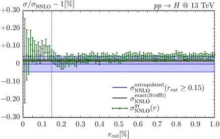
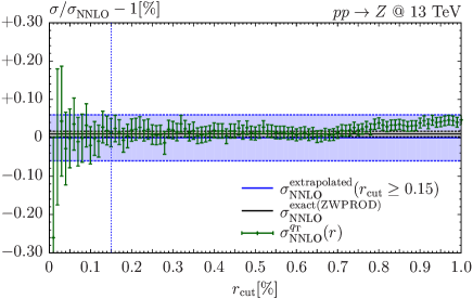
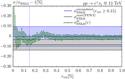
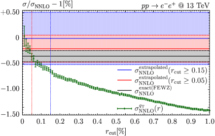
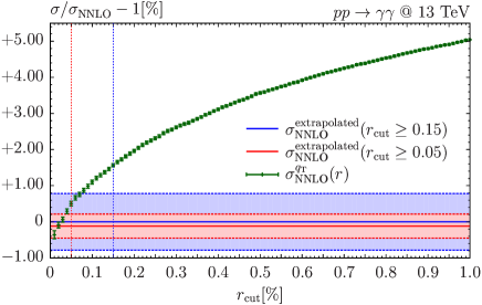
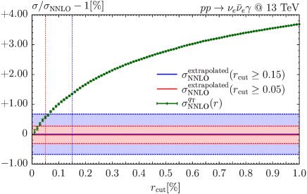
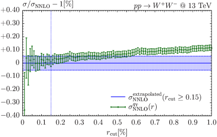
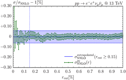
Figure 2: Dependence of the NNLO cross sections on $r_{\mathrm{cut}}{}$ for various processes. The NNLO results at fixed values of $r_{\mathrm{cut}}$ are normalized to the $r_{\mathrm{cut}}\to 0$ extrapolation obtained by using $r_{\mathrm{cut}}\geq 0.15$%. The blue band represents the combined numerical and extrapolation uncertainty. For processes with a large $r_{\mathrm{cut}}$ dependence, the extrapolated result and uncertainty obtained by using $r_{\mathrm{cut}}\geq 0.05$% is shown in red. Where available, $r_{\mathrm{cut}}$-independent reference results are black.

Our results for the $r_{\mathrm{cut}}$ dependence of a representative set of processes are shown in Figure 2. Before commenting the various plots we provide some general explanation. The central values of the green bars represent the NNLO cross section calculated at the respective fixed $r_{\mathrm{cut}}$ values, $r_{\mathrm{cut}}{}\in[0.01\%;1\%]$ in steps of $0.01\%$, and their sizes denote the numerical uncertainties. Our reference prediction, computed with the default Matrix setup, is the $r_{\mathrm{cut}}{}\rightarrow 0$ extrapolation obtained from the values $r_{\mathrm{cut}}{}\geq 0.15\%$, shown as a blue solid line. A vertical blue dotted line at $r_{\mathrm{cut}}{}=0.15\%$ indicates the lowest value used for this extrapolation. The blue uncertainty band is obtained by combining the numerical and extrapolation uncertainties and corresponds to the on-screen output of Matrix. When the $r_{\mathrm{cut}}$ dependence is strong, we also show the Matrix result extrapolated from $r_{\mathrm{cut}}{}\geq 0.05\%$ values as a red solid line with a red band, with its uncertainty computed analogously to the blue band. Where available, NNLO results obtained either from analytical calculations or from alternative NNLO numerical programs are reported as black lines, while the grey band shows their numerical integration error. All the results are reported as relative deviations from the reference prediction in percent.

We start our discussion from the first two plots in Figure 2, which refer to the inclusive on-shell production of a Higgs (left) and a $Z$ boson (right), respectively. In both cases the NNLO cross sections turn out to be extremely stable with respect to $r_{\mathrm{cut}}$: Almost all fixed-$r_{\mathrm{cut}}$ results deviate by less than one permille from the default $r_{\mathrm{cut}}{}\rightarrow 0$ prediction, and all fixed-$r_{\mathrm{cut}}$ results are compatible with the extrapolated result within their numerical uncertainties. The high stability with respect to $r_{\mathrm{cut}}$ in these cases would justify choosing essentially any $r_{\mathrm{cut}}{}$ value in the given range to provide a reasonable prediction for the NNLO cross section. Our default choice to use $r_{\mathrm{cut}}{}\geq 0.15$% to obtain the $r_{\mathrm{cut}}\rightarrow 0$ extrapolation appears to be a sound compromise between a sufficiently low $r_{\mathrm{cut}}$ value and a good numerical convergence. The blue band constitutes a reasonable estimate of the remaining extrapolation uncertainty of our reference result. Since no cuts have been applied, our results can be compared with available analytic computations of the inclusive Higgs and $Z$ production cross sections. Such results are obtained with SusHi [110] for Higgs boson production, and with ZWPROD [2, 3] for $Z$-boson production, and are reported in Figure 2 by the black solid lines with grey numerical error bands. The agreement is excellent and confirms that with Matrix we control these computations at the sub-permille level.

The next process we consider is $pp\rightarrow e^{+}\nu_{e}$ via an off-shell $W^{+}$ boson (third plot in Figure 2). The $r_{\mathrm{cut}}$ dependence is similar to the case of on-shell Higgs and $Z$ production with all fixed-$r_{\mathrm{cut}}$ results deviating not more than about one permille from the extrapolated result. We therefore conclude that the stability fully justifies our reference prediction and that its blue uncertainty band, which is slightly larger than for the on-shell processes discussed before, gives a reasonable estimate of the uncertainty due to the $r_{\mathrm{cut}}$ dependence of the cross section. In the same plot we also report the result obtained with FEWZ [52], depicted by a solid black line with grey error bands. The Matrix and FEWZ results are fully consistent within the respective numerical uncertainties. A similar level of agreement is obtained with the program NNLOjet [117]. Since both FEWZ and NNLOjet are based on fully independent subtraction schemes, the above agreement can be considered as an important mutual consistency check of the three NNLO calculations.

Next, we discuss the dilepton production process $pp\rightarrow e^{-}e^{+}$, which, in our default setup, exhibits a rather large $r_{\mathrm{cut}}$ dependence. This is illustrated in the fourth plot of Figure 2. As discussed in Section 5, the strong $r_{\mathrm{cut}}$ dependence can be traced back to the presence of perturbative instabilities [111] affecting the fixed-order computation in the case of symmetric $p_{T}$ cuts. We have explicitly tested that if we change our default setup from $p_{T,\ell}>25$ GeV to $p_{T,e^{-}}>25$ GeV and $p_{T,e^{+}}>24$ GeV, we get a stable $r_{\mathrm{cut}}$ dependence. If we change this setup by letting the cut on $p_{T,e^{+}}$ approach $25$ GeV, the $r_{\mathrm{cut}}$ dependence of the cross section becomes increasingly stronger. We also point out that, if we remove the lepton $p_{T}$ thresholds completely or choose them as small as $p_{T,\ell}>5$ GeV, we obtain a flat $r_{\mathrm{cut}}$ dependence of the cross section. The sizeable $r_{\mathrm{cut}}$ dependence implies a larger uncertainty in the $r_{\mathrm{cut}}\to 0$ extrapolation. We indeed see that by using the default setup the estimated uncertainty, represented by the blue band, is about $\pm 0.5\%$. By reducing the minimum $r_{\mathrm{cut}}$ value to $0.05\%$, we reduce the extrapolation uncertainty by about a factor of 2 (red band) and we obtain a fully consistent result with the one obtained from $r_{\mathrm{cut}}\geq 0.15\%$. This is a strong indication that the extrapolation procedure is robust and provides a reasonable estimate of the ensuing uncertainty. In the same plot we report the result obtained with FEWZ: the agreement with the extrapolated results is excellent. A similar level of agreement is obtained with NNLOjet. As in the previous cases, the agreement of NNLO predictions obtained with fully independent methods confirms the robustness of the results that can be obtained with Matrix. We remark that this conclusion holds also in a case, like the one of dilepton production with symmetric cuts, in which a fixed-order computation is challenged.

In terms of the $r_{\mathrm{cut}}$ dependence of their cross sections, processes with an isolated photon in the final state suffer from large power-suppressed corrections. Since the case of $W\gamma$ production was discussed in Ref. [31], here we consider diphoton and $Z\gamma$ production with the $Z$ boson decaying to a neutrino pair. The corresponding results are shown in the fifth and sixth plot in Figure 2, respectively. Looking at our extrapolated reference results for $r_{\mathrm{cut}}{}\geq 0.15$% and $r_{\mathrm{cut}}{}\geq 0.05$%, we see that they are nicely consistent with the behaviour of the numerical results below the respective minimal $r_{\mathrm{cut}}$ value and that they are in neat mutual agreement. In particular, the result at the lowest $r_{\mathrm{cut}}$ value $r_{\mathrm{cut}}{}=0.01$% is consistent with both the red and blue bands in all cases.

It is clear that, for dilepton, diphoton and $Z\gamma$ production, the extrapolation $r_{\mathrm{cut}}\rightarrow 0$ of runs with $r_{\mathrm{cut}}{}\geq 0.15$% allows us to control the uncertainty of our NNLO predictions at the $0.5-1$% level. If the minimal $r_{\mathrm{cut}}$ value is decreased to $r_{\mathrm{cut}}^{\mathrm{min}}{}=0.05$%, the ensuing uncertainty is reduced to few permille. We have explicitly checked that this picture is common to all processes involving photons. We conclude that, taking into account the estimated $r_{\mathrm{cut}}$ uncertainties, we obtain consistent predictions for all these processes.

The last two plots in Figure 2 are representative $r_{\mathrm{cut}}$-dependence plots for on- and off-shell diboson production: The first one shows on-shell $W^{+}W^{-}$ production, and the second one off-shell $ZZ$ production in the $2\ell 2\nu^{\prime}$ decay channel. These plots feature to a large extent the same behaviour as observed for on-shell Higgs and vector-boson production processes: In general, the NNLO cross section is very stable with respect to $r_{\mathrm{cut}}$ over two orders of magnitude. The $r_{\mathrm{cut}}$ dependence of the $W^{+}W^{-}$ cross section seems to have a very slight slope, which, however, is perfectly modelled by the extrapolation. Our default choice of the minimal $r_{\mathrm{cut}}$ value leads to a reasonable reference result with the estimated uncertainties being meaningful and in some cases even a bit conservative.

In summary, for most of the processes implemented in the first release of Matrix, NNLO predictions can generally be controlled at the one permille level (or better). For processes with a large $r_{\mathrm{cut}}$ dependence like those involving photons or Drell–Yan dilepton pairs, fiducial cross sections can be computed with uncertainties of few permille by using the setting switch_qT_accuracy = 1. This accuracy should be sufficient for all practical purposes.

7 Summary

In this paper we have introduced the new computational framework Matrix[1], which allows a user to produce NNLO QCD predictions for a wide class of hadron-collider processes. Using the $q_{T}$-subtraction formalism, our computations are fully differential in the phase space of the final-state particles and of the associated QCD radiation, thereby enabling the evaluation of arbitrary IR safe observables. Since our implementation is completely general, it is applicable to the computation of NNLO corrections to any process with colourless final states. The list of available processes is therefore limited only by the availability of two-loop amplitudes to the Born-level processes. The first Matrix release involves $2\to 1$ and $2\to 2$ hadronic reactions with Higgs and vector bosons in the final state. In particular, we consider final states with two, three and four leptons (plus missing energy) from the decays of the vector bosons, and we account for all resonant and non-resonant diagrams with off-shell effects and spin correlations. This enables the evaluation of cross sections with realistic cuts to define any fiducial volume.

We have presented a detailed description of the first release of the Matrix code. Besides the theoretical framework and the tools Matrix is based on, we have focused on the technical aspects relevant for a user to produce fully differential NNLO results. Matrix features automatic compilation and running through dedicated scripts. The most popular clusters are preconfigured and can be simply selected by the user. Having specified a target precision and a desired runtime per job, the code automatically determines the required parallelization in each run. In combination with the fast numerical multi-channel integration offered by Munich, this allows us to obtain accurate NNLO results even for the most complicated of the available processes on a middle-sized cluster in less than a couple of days, simpler processes being significantly faster. With every run Matrix provides not only the central prediction, but automatically evaluates the effect of independent factorization- and renormalization-scale variations in order to obtain an estimate of the perturbative uncertainties at each order. Furthermore, by simultaneously computing NNLO cross sections at several values of the $q_{T}$-subtraction parameter $r_{\mathrm{cut}}$, Matrix performs an extrapolation $r_{\mathrm{cut}}\rightarrow 0$ of the integrated cross section in order to provide its final prediction that includes an extrapolation uncertainty. Such procedure allows us to offer a robust estimate of the systematic uncertainty due to the $q_{T}$-subtraction procedure. Both scale variations and the $r_{\mathrm{cut}}$ extrapolation procedure are fully automated within Matrix without the need of extra computing power.

In particular for processes with a large $r_{\mathrm{cut}}$ dependence, such as dilepton production or processes with isolated photons, Matrix is able to significantly improve over predictions computed at fixed $r_{\mathrm{cut}}$ values by performing the $r_{\mathrm{cut}}\to 0$ extrapolation. Besides an improved accuracy in the central prediction, our procedure includes a conservative estimate of systematic uncertainties, which allows the user to control the precision of these processes at the level of few permille, when using corresponding settings.

We have discussed in detail all relevant Matrix input cards accessible to the user. Besides standard settings applicable to all processes, information specific to each individual process has been provided, such as suitable dynamic scales which are predefined for certain processes and process-specific cuts. The latter facilitate the restriction of the phase space to fiducial volumes as defined by the LHC experiments. In combination with a general way to define distributions, this enables the possibility to compute fiducial cross sections and distributions that can be directly compared to unfolded experimental data.

Reference predictions for the integrated cross sections of all processes available in Matrix have been provided at LO, NLO and NNLO in the default setups. For the NNLO cross section we have quoted predictions for a fixed value $r_{\mathrm{cut}}=0.15$% and the final NNLO result after performing the extrapolation $r_{\mathrm{cut}}\rightarrow 0$. We have studied the impact of radiative corrections for each of these processes as well as the impact of the loop-induced $gg$ component, where applicable. The impact of NLO and NNLO QCD corrections is generally large. While NLO corrections typically range between $30\%-100\%$, NNLO corrections are still as large as $3\%-30\%$ for the processes and scenarios we have considered. The size of radiative corrections is typically widely un-affected if only fiducial cuts for particle identification, like transverse-momentum thresholds, geometric (pseudo-)rapidity ranges or isolation cuts are applied (see, e.g., inclusive on-shell $ZZ$ production and off-shell $ZZ\to 4\ell$ production in a $ZZ$ signal region). This is in general no longer true if the considered cuts modify the dominant resonance structures (e.g. $ZZ\to 4\ell$ production in the $H\to ZZ$ background region). If real radiation is restricted, in particular by a veto against jets, the size of higher-order corrections is strongly suppressed, and NLO and NNLO $K$ factors can be very different as compared to the inclusive phase-space (see, e.g., inclusive on-shell $W^{+}W^{-}$ production and off-shell $WW\to 2\ell 2\nu$ production, which requires a jet veto to suppress the top-quark backgrounds).

Scale variations tend to underestimate the uncertainty from missing higher-order contributions at LO, and also widely at NLO. This is due to the fact that vector-boson and vector-boson pair production processes are driven by $q\bar{q}$ initial states at LO ($gg$ initial states in case of Higgs boson production). The $gq$ channel opens up only at NLO, and NNLO is the first order where all partonic channels are contributing. As a consequence, in most of the cases NNLO uncertainties obtained through scale variations should provide the correct order of magnitude of yet un-calculated perturbative QCD contributions. When NNLO corrections are particularly large, as in the case of diphoton production, a more conservative estimate of missing higher-order contributions can be obtained by considering the difference with the previous order.

All the vector-boson pair production processes with an electrically neutral final state include a loop-induced $gg$ contribution at NNLO. Its size strongly depends on the considered process and can range between roughly $10\%$ and $60\%$ of the NNLO corrections. In cases where radiative corrections are suppressed by a jet veto, since the $gg$ component is not affected due to its Born-level kinematics, it may provide the dominant NNLO contribution. As the $gg$ component is effectively only LO accurate, scale variations might underestimate the actual size of its missing perturbative corrections in some cases.

To conclude, we believe that the numerical tool presented in this paper will be highly valuable for the high-energy community. Several experimental studies have already used the results obtained with Matrix for data–theory comparison in SM measurements (see, e.g., Refs. [118, 119, 120, 121, 122, 123, 124, 125, 126, 127, 128, 129, 130, 131, 132, 107, 133, 134, 135, 136]) and for background estimates in various new-physics searches. Matrix[1] can be used to produce benchmark predictions for a wide range of processes relevant both for SM measurements and as backgrounds to Higgs and new-physics searches. Extensions of the code to include additional processes, the inclusion of further perturbative contributions (e.g. NLO corrections to the $gg$ channel or EW corrections) as well as the resummation of certain classes of logarithmic contributions are left for future work.

Acknowledgements.

We are grateful to Dirk Rathlev for his contributions at the beginning of the Matrix project. We would like to thank Stefano Catani for comments on the manuscript and Alexander Huss for providing cross checks for the Drell–Yan processes with NNLOjet. We are indebted to Jonas Lindert, Philipp Maierhöfer and Stefano Pozzorini for their continuous support on OpenLoops. We thank Thomas Gehrmann, Andreas von Manteuffel and Lorenzo Tancredi for providing us with private implementations of the two-loop amplitudes to on-shell $W^{+}W^{-}$ and $ZZ$ production. This research was supported in part by the Munich Institute for Astro- and Particle Physics (MIAPP) of the DFG cluster of excellence ”Origin and Structure of the Universe“, by the Swiss National Science Foundation (SNF) under contracts CRSII2-141847, 200020-169041 and by the Research Executive Agency (REA) of the European Union under the Grant Agreement number PITN–GA–2012–316704 (HiggsTools). The work of MW is supported by the ERC Consolidator Grant 614577 HICCUP.

Appendix Appendix A Predefined cuts

In this Appendix the process-dependent cuts introduced in Section 4.2 are explained in more detail. It can be used as a dictionary since the respective cuts in Section 4.2 contain interactive links to their explanations in Table LABEL:tab:predefinedcuts.

Table 11: Explanations of the pre-defined cuts available in the various Matrix processes. See Section 4.2 for which cuts belong to which process.

user_switch	description
user_cut
lepton_identification	Switch to change between different identification procedures of $Z$ and $W$ bosons in the same-flavour channels of $ZZ$ and $WZ$ production. See Section 4.2.4.4 and Section 4.2.4.9 for details.
M_leplep	Switch for cuts on invariant mass $m_{\ell\ell}$ of all possible lepton pairs.
min_M_leplep	Minimal requirement $m_{\ell\ell}>$ min_M_leplep for all lepton pairs.
max_M_leplep	Maximal requirement $m_{\ell\ell}<$ max_M_leplep for all lepton pairs.
M_leplep_OSSF	Switch for cuts on invariant mass $m_{\ell^{-}\ell^{+}}$ of opposite-sign, same-flavour (OSSF) lepton pairs.
min_M_leplep_OSSF	Minimal requirement $m_{\ell^{-}\ell^{+}}>$ min_M_leplep_OSSF for OSSF pairs.
max_M_leplep_OSSF	Maximal requirement $m_{\ell^{-}\ell^{+}}<$ max_M_leplep_OSSF for OSSF pairs.
min_M_Z1_OSSF	Minimal requirement $m_{\ell^{-}\ell^{+}}>$ min_M_Z1_OSSF for OSSF pair closer to $m_{Z}$.
max_M_Z1_OSSF	Maximal requirement $m_{\ell^{-}\ell^{+}}<$ max_M_Z1_OSSF for OSSF pair closer to $m_{Z}$.
M_Zrec	Switch for cuts on invariant mass $m_{\ell^{-}\ell^{+}}$ of lepton pairs associated with $Z$ bosons.
min_M_Zrec	Minimal requirement $m_{\ell^{-}\ell^{+}}>$ min_M_Zrec for (reconstructed) $Z$ bosons.
max_M_Zrec	Maximal requirement $m_{\ell^{-}\ell^{+}}<$ max_M_Zrec for (reconstructed) $Z$ bosons.
delta_M_Zrec_MZ	Switch for cuts on absolute difference between invariant mass $m_{\ell^{-}\ell^{+}}$ of lepton pairs associated with $Z$ bosons and the $Z$-boson mass.
max_delta_M_Zrec_MZ	Maximal requirement $|m_{\ell^{-}\ell^{+}}-m_{Z}|<$ max_delta_M_Zrec_MZ for (reconstructed) $Z$ bosons.
delta_M_lepleplep_MZ	Switch for cuts on absolute difference between invariant mass $m_{\ell\ell\ell}$ of 3-lepton system and the $Z$-boson mass.
min_delta_M_lepleplep_MZ	Minimal requirement $|m_{\ell\ell\ell}-m_{Z}|>$ min_delta_M_lepleplep_MZ.
M_4lep	Switch for cuts on invariant mass $m_{\ell\ell\ell\ell}$ of 4-lepton system.
min_M_4lep	Minimal requirement $m_{\ell\ell\ell\ell}>$ min_M_4lep for 4-lepton system.
max_M_4lep	Maximal requirement $m_{\ell\ell\ell\ell}<$ max_M_4lep for 4-lepton system.
min_delta_M_4lep	Minimal requirement $|m_{\ell\ell\ell\ell}-m_{Z}|>$ min_delta_M_4lep for 4-lepton system.
max_delta_M_4lep	Maximal requirement $|m_{\ell\ell\ell\ell}-m_{Z}|<$ max_delta_M_4lep for 4-lepton system.
M_leplepnunu	Switch for cuts on invariant mass $m_{\ell\ell\nu\nu}$ of 2-lepton–2-neutrino system.
min_M_leplepnunu	Minimal requirement $m_{\ell\ell\nu\nu}>$ min_delta_M_leplepnunu for 2$\ell$2$\nu$ system.
max_M_leplepnunu	Maximal requirement $m_{\ell\ell\nu\nu}<$ max_delta_M_leplepnunu for 2$\ell$2$\nu$ system.
min_delta_M_leplepnunu	Min. requirement $|m_{\ell\ell\nu\nu}-m_{Z}|>$ min_delta_M_leplepnunu for 2$\ell$2$\nu$ system.
max_delta_M_leplepnunu	Max. requirement $|m_{\ell\ell\nu\nu}-m_{Z}|<$ max_delta_M_leplepnunu for 2$\ell$2$\nu$ system.
pT_leplep	Switch for cuts on transverse momentum of lepton pair $p_{T,\ell\ell}$.
min_pT_leplep	Minimal requirement $p_{T,\ell\ell}>$ min_pT_leplep for lepton pair.
pT_lep_1st	Switch for cuts on transverse momentum of hardest lepton $p_{T,\ell_{1}}$.
min_pT_lep_1st	Minimal requirement $p_{T,\ell_{1}}>$ min_pT_lep_1st for hardest lepton.
pT_lep_2nd	Switch for cuts on transverse momentum of second-hardest lepton $p_{T,\ell_{2}}$.
min_pT_lep_2nd	Minimal requirement $p_{T,\ell_{2}}>$ min_pT_lep_2nd for second-hardest lepton.
lepton_cuts	Switch for cuts on transverse momentum of (second-)hardest lepton $p_{T,\ell_{1}}$($p_{T,\ell_{2}}$).
min_pT_lep_1st	Minimal requirement $p_{T,\ell_{1}}>$ min_pT_lep_1st for hardest lepton.
min_pT_lep_2nd	Minimal requirement $p_{T,\ell_{2}}>$ min_pT_lep_2nd for second-hardest lepton.
leading_lepton_cuts	Switch for flavour-dependent cuts on hardest-lepton transverse momentum $p_{T,\ell_{1}}$.
min_pT_1st_if_e	Minimal requirement $p_{T,\ell_{1}}>$ min_pT_1st_if_e if hardest lepton is electron.
min_pT_1st_if_mu	Minimal requirement $p_{T,\ell_{1}}>$ min_pT_1st_if_mu if hardest lepton is muon.
lepZ_cuts	Switch for cuts on transverse momentum of (second-)hardest lepton associated with $Z$-boson decay $p_{T,\ell_{Z,1}}\,(p_{T,\ell_{Z,2}})$.
min_pT_lepZ_1st	Minimal requirement $p_{T,\ell_{Z,1}}>$ min_pT_lepZ_1st for hardest lepton of $Z$.
min_pT_lepZ_2nd	Minimal requirement $p_{T,\ell_{Z,2}}>$ min_pT_lepZ_2nd for second-hardest lepton of $Z$.
lepW_cuts	Switch for cuts on lepton associated with $W$-boson decay.
min_pT_lepW	Minimal requirement $p_{T,\ell_{W}}>$ min_pT_lepW for lepton from $W$-boson decay.
max_eta_lepW	Minimal requirement $\eta_{\ell_{W}}<$ max_eta_lepW for lepton from $W$-boson decay.
R_leplep	Switch for cuts on lepton separation in $\Delta R_{\ell\ell}=\sqrt{\Delta y_{\ell\ell}^{2}+\Delta\phi_{\ell\ell}^{2}}$.
min_R_leplep	Minimal requirement $\Delta R_{\ell\ell}>$ min_R_leplep for all lepton pairs.
R_lepZlepZ	Switch for cuts on separation between leptons associated with $Z$-boson decay in $\Delta R_{\ell_{Z}\ell_{Z}}=\sqrt{\Delta y_{\ell_{Z}\ell_{Z}}^{2}+\Delta\phi_{\ell_{Z}\ell_{Z}}^{2}}$.
min_R_lepZlepZ	Minimal requirement $\Delta R_{\ell_{Z}\ell_{Z}}>$ min_R_lepZlepZ for leptons of $Z$ decay.
R_lepZlepW	Switch for cuts on separation between leptons associated with $Z$-boson decay and lepton associated with $W$-boson decay in $\Delta R_{\ell_{Z}\ell_{W}}=\sqrt{\Delta y_{\ell_{Z}\ell_{W}}^{2}+\Delta\phi_{\ell_{Z}\ell_{W}}^{2}}$.
min_R_lepZlepW	Minimal requirement $\Delta R_{\ell_{Z}\ell_{W}}>$ min_R_lepZlepW for leptons of $Z$ and $W$ decay.
phi_leplep	Switch for cuts on azimuthal separation $\Delta\phi_{\ell\ell}$ between all lepton pairs.
min_phi_leplep	Minimal requirement $\Delta\phi_{\ell\ell}>$ min_phi_leplep for all lepton pairs.
phi_leplep_nunu	Switch for cuts on azimuthal separation $\Delta\phi_{\ell\ell,\nu\nu}$ between the transverse-momentum vectors of the 2-lepton system $\boldsymbol{p}_{\rm\boldsymbol{T},\ell\ell}$ and the missing energy $\mathbf{p_{T}^{\text{miss}}}$.
min_phi_leplep_nunu	Minimal requirement $\Delta\phi_{\ell\ell,\nu\nu}>$ min_phi_leplep_nunu.
electron_cuts	Switch for cuts on transverse momentum of (second-)hardest electron $p_{T,e_{1}}$($p_{T,e_{2}}$).
min_pT_e_1st	Minimal requirement $p_{T,e_{1}}>$ min_pT_e_1st for hardest electron.
min_pT_e_2nd	Minimal requirement $p_{T,e_{2}}>$ min_pT_e_2nd for second-hardest electron.
muon_cuts	Switch for cuts on transverse momentum of (second-)hardest muon $p_{T,\mu_{1}}$($p_{T,\mu_{2}}$).
min_pT_mu_1st	Minimal requirement $p_{T,\mu_{1}}>$ min_pT_mu_1st for hardest muon.
min_pT_mu_2nd	Minimal requirement $p_{T,\mu_{2}}>$ min_pT_mu_2nd for second-hardest muon.
gap_eta_e	Switch for detector gap in absolute pseudo-rapidity $|\eta_{e}|$ of electrons.
gap_min_eta_e	Start of the gap, keeping only events with $|\eta_{e}|<$ gap_min_eta_e.
gap_max_eta_e	End of the gap, keeping only events with $|\eta_{e}|>$ gap_max_eta_e.
M_gamgam	Switch for cuts on invariant mass $m_{\gamma\gamma}$ of photon pairs.
min_M_gamgam	Minimal requirement $m_{\gamma\gamma}>$ min_M_gamgam for photon pairs.
max_M_gamgam	Maximal requirement $m_{\gamma\gamma}<$ min_M_gamgam for photon pairs.
pT_gam_1st	Switch for cuts on transverse momentum of hardest photon $p_{T,\gamma_{1}}$.
min_pT_gam_1st	Minimal requirement $p_{T,\gamma_{1}}>$ min_pT_gam_1st for hardest photon.
R_gamgam	Switch for cuts on photon separation in $\Delta R_{\gamma\gamma}=\sqrt{\Delta y_{\gamma\gamma}^{2}+\Delta\phi_{\gamma\gamma}^{2}}$.
min_R_gamgam	Minimal requirement $\Delta R_{\gamma\gamma}>$ min_R_gamgam for photon pairs.
gap_eta_gam	Switch for detector gap in absolute pseudo-rapidity $|\eta_{\gamma}|$ of photons.
gap_min_eta_gam	Start of the gap, keeping only events with $|\eta_{\gamma}|<$ gap_min_eta_gam.
gap_max_eta_gam	End of the gap, keeping only events with $|\eta_{\gamma}|>$ gap_max_eta_gam.
M_lepgam	Switch for cuts on invariant mass $m_{\ell\gamma}$ of lepton–photon pairs.
min_M_lepgam	Minimal requirement $m_{\ell\gamma}>$ min_M_lepgam for lepton–photon pairs.
R_lepgam	Switch for cuts on lepton–photon separation in $\Delta R_{\ell\gamma}=\sqrt{\Delta y_{\ell\gamma}^{2}+\Delta\phi_{\ell\gamma}^{2}}$.
min_R_lepgam	Minimal requirement $\Delta R_{\ell\gamma}>$ min_R_lepgam for lepton–photon pairs.
R_lepjet	Switch for cuts on lepton–jet separation in $\Delta R_{\ell j}=\sqrt{\Delta y_{\ell j}^{2}+\Delta\phi_{\ell j}^{2}}$.
min_R_lepjet	Minimal requirement $\Delta R_{\ell j}>$ min_R_lepjet for lepton–jet pairs.
lep_iso	Switch for special isolation of lepton–lepton and lepton–parton pairs, as used for example in the $ZZ$ Higgs background, see Ref. [137]. For each lepton $i$ we compute the sum of the transverse momenta over all leptons and partons in a certain $R$ cone around $i$ and take the ratio to its transverse momentum. All events are discarded where this ratio is below a certain threshold: $$\left.\sum_{\begin{subarray}{c}j\in\{\ell,\text{partons}\}\\ \text{ with }\Delta R_{ij}<\delta_{0}\end{subarray}}p_{T,j}\middle/p_{T,i}\right.<\epsilon$$
lep_iso_delta_0	$\delta_{0}$ in the formula above.
lep_iso_epsilon	$\epsilon$ in the formula above.
R_ejet	Switch for cuts on electron–jet separation in $\Delta R_{ej}=\sqrt{\Delta y_{ej}^{2}+\Delta\phi_{ej}^{2}}$.
min_R_ejet	Minimal requirement $\Delta R_{ej}>$ min_R_ejet for electron–jet pairs.
R_gamjet	Switch for cuts on photon–jet separation in $\Delta R_{\gamma j}=\sqrt{\Delta y_{\ell j}^{2}+\Delta\phi_{\ell j}^{2}}$.
min_R_gamjet	Minimal requirement $\Delta R_{\gamma j}>$ min_R_gamjet for photon–jet pairs.
mT_CMS	Switch for cuts on transverse mass $m_{T,W}$ of $W$ boson as defined by CMS [138].
min_mT_CMS	Minimal requirement $m_{T,W}>$ min_mT_CMS for the $W$ boson.
pT_W	Switch for cuts on transverse momentum $p_{T,\ell\nu_{\ell}}$ of (identified) $W$ bosons.
min_pT_W	Minimal requirement $p_{T,\ell\nu_{\ell}}>$ min_pT_W for (identified) $W$ bosons.
max_pT_W	Maximal requirement $p_{T,\ell\nu_{\ell}}<$ max_pT_W for (identified) $W$ bosons.
MT_Wrec	Switch for cuts on transverse mass $m_{T,\ell\nu_{\ell}}$ of (identified) $W$ bosons, defined by $$m_{T,\ell\nu_{\ell}}=\sqrt{\left(E_{T,\ell}+E_{T,\nu_{\ell}}\right)^{2}-\left(p_{T,\ell\nu_{\ell}}\right)^{2}}\quad\mathrm{with}\quad(E_{T,x})^{2}=m_{x}^{2}+(p_{T,x})^{2}$$
min_MT_Wrec	Minimal requirement $m_{T}^{\ell\nu_{\ell}}>$ min_mT_Wrec for (identified) $W$ bosons.
rel_pT_miss	Switch for cuts on the relative missing transverse momentum $p_{T}^{\text{miss,rel}}$, which is defined as $p_{T}^{\text{miss}}\times\sin|\Delta\phi|$, where $\Delta\phi$ is the azimuthal separation between $\mathbf{p_{T}^{\text{miss}}}$ and the momentum of the closest lepton, see Ref. [128].
min_rel_pT_miss	Minimal requirement $p_{T}^{\text{miss,rel}}>$ min_rel_pT_miss.

Appendix Appendix B Modifications of the C++ code (advanced user)

The user is generally advised to contact the authors if he/she is interested in changing any parts of the C++ code in order to define new dynamic scales, fiducial cuts or distributions. Below we provide some general guidance on how such implementations can be realized in the C++ code. Any changes of the C++ code require recompilation of the relevant process. This can be done with the matrix script, but in certain cases it might be simpler to use directly the Makefile the matrix script has created during the initial compilation of a process with ID ${process_id}, by typing

⬇

$ make ${process_id}

This enables recompilation without cleaning the whole process and without checking again whether all the relevant libraries are correctly installed.

B.1 General C++ commands

B.1.1 Access to particle groups

In the C++ routines for the user-defined scales and cuts one has access to all particle groups listed in Figure 3 and the ones defined by the user, see below. As discussed before, the particle groups are ordered in the transverse momentum of the particles and can be accessed via PARTICLE("${particle_group}")[index], where ${particle_group} is one of the particle groups defined in Table 3 or the user-defined ones, and index indicates the position in the $p_{T}{}$-ordering of the group starting from the hardest one at index = 0.

For example, the hardest lepton can be accessed via

language=, backgroundcolor=, basicstyle=, keywordstyle=, stringstyle=, commentstyle=, basicstyle=, frame=single

⬇

particle hardest_lepton = PARTICLE("lep")[0];

The particle class itself has various predefined class variables that can be directly used. For example, the $p_{T}$ or squared invariant mass can be determined as follows:

⬇

double pT_hardest_lepton = PARTICLE("lep")[0].pT;

double m2_hardest_lepton = PARTICLE("lep")[0].m2;

These can also determined via the full four-vector that has certain predefined functions and can be used as follows:

⬇

fourvector fourvector_of_hardest_lepton = PARTICLE("lep")[0].momentum;

double pT_hardest_lepton = fourvector_of_hardest_lepton.pT();

double m2_hardest_lepton = fourvector_of_hardest_lepton.m2();

or similar functions for other observables, such as rapidity and pseudo-rapidity

⬇

double y_hardest_lepton = PARTICLE("lep")[0].momentum.rapidity();

double eta_hardest_lepton = PARTICLE("lep")[0].momentum.eta();

It is important to note that the four-vectors of the particles can be simply added to define a new four-vector, where the same functions can be used. For example, the transverse mass ($\sqrt{m^{2}+p_{T}^{2}}$) of the system of the lepton pair (hardest and second-hardest lepton) can be simply computed by

⬇

fourvector fourvector_of_leplep = PARTICLE("lep")[0].momentum+PARTICLE("lep")[1].momentum;

double mT_leplep = fourvector_of_leplep.ET();

Similarly, one may also directly sum two objects of type particle to define a new particle whose momentum corresponds to the sum. Thus, it would be equivalent to compute the transverse mass of the system of the lepton pair by using

⬇

particle leplep = PARTICLE("lep")[0] + PARTICLE("lep")[1];

double mT_leplep = leplep.ET;

Finally, if a certain observable one may want to compute is neither predefined in the particle nor the fourvector class, one can always access the momenta directly by using

⬇

fourvector fourvector_of_hardest_lep = PARTICLE("lep")[0].momentum;

double E_hardest_lep = fourvector_of_hardest_lepton.x0();

double x_hardest_lep = fourvector_of_hardest_lepton.x1();

double y_hardest_lep = fourvector_of_hardest_lepton.x2();

double z_hardest_lep = fourvector_of_hardest_lepton.x3();

and compute the desired observable from the explicit momentum components.

B.1.2 Access to user-defined parameters

In the file parameter.dat three types of user-defined parameters can be added, which are available in the C++ code and can be directly accessed throughout the process-specific C++ files inside the folder MATRIX_v1.0.0/prc/${process_id}/user.

• An integer-valued user parameter is added via

  ⬇

  user_switch my_integer_parameter = 1

  to the file parameter.dat and is accessed in the C++ code by

  ⬇

  static int my_integer = USERSWITCH("my_integer_parameter");

  Such switches are useful in many respects, two already used examples are to turn on and off cuts, or to choose between different identification procedures.

• A real-valued user parameter is added via

  ⬇

  user_cut my_real_parameter = 1.23

  to the file parameter.dat and is accessed in the C++ code by

  ⬇

  static double my_real = USERCUT("my_real_parameter");

  Such real parameters are useful in many respects, the most important example is their use to define and implement cuts that can be changed later from the file parameter.dat without recompilation of the code.

• Finally, a new particle (group) can be defined by adding

  ⬇

  user_particle my_own_particle = my_own_particle

  to the file parameter.dat. Only if defined this way, it can be filled in the C++ code,

  ⬇

  USERPARTICLE("my_own_particle").push_back(PARTICLE("lep")[0] + PARTICLE("lep")[1]);

  which would add a particle whose momentum is the sum of the hardest and second-hardest lepton to the user-defined particle group my_own_particle. If a user-defined particle group is filled with more than one particle, the usual $p_{T}$-ordering is done automatically before the respective particle group is used in scales, cuts or distributions. Note that a USERPARTICLE may only be filled in a certain position of the code, see below in Appendix B.2, and that it can be accessed later like all other particle groups via the container PARTICLE.

B.2 Definition of a new particle group

The predefined particle groups are sufficient for most practical cases. However, the user is allowed to define his own particle group by filling the respective four-vectors. This can be very useful if an intermediate particle cannot be unambiguously reconstructed, like in the case of the SF channel in $ZZ$(or $W^{\pm}Z$) production, where an identification procedure is needed for the $Z$ (and the $W$) bosons. As described in Sections 4.2.4.4 and 4.2.4.9, such definition of process-specific particle groups is done intrinsically for these two processes following different identification procedures used by ATLAS and CMS. In the following we describe the necessary steps for a user to add his own definition of a particle group to any process.

The relevant C++ file is MATRIX_v1.0.0/prc/${process_id}/user/specify.particles.cxx to fill user-defined particles. As described above, one has to add the definition of a new particle group to the file parameter.dat. After that the respective particle group exists as an empty array of objects of type particle inside the C++ code, which must be filled by appending at least one object of type particle to the array.

Let us give a simple example: A new particle group should be filled depending on the value of an integer switch with either the hardest lepton or the second-hardest lepton. The relevant input in the file parameter.dat would look like

⬇

user_particle relevant_lepton = relevant_lepton # lepton, depending on switch_lepton

user_switch switch_lepton = 0 # (0) hardest lepton, (1) second-hardest lepton

and the relevant C++ code in the specify.particles.cxx would be

⬇

...

static int switch_lepton = USERSWITCH("switch_lepton");

if (switch_lepton == 0){

USERPARTICLE("relevant_lepton").push_back(PARTICLE("lep")[0]);

}

else if (switch_lepton == 1){

USERPARTICLE("relevant_lepton").push_back(PARTICLE("lep")[1]);

}

else {

logger << LOG_ERROR << "ERROR: switch_lepton = " << switch_lepton << "; allowed values: 0, 1" << endl;

assert(false);

}

...

Bear in mind that after definition of a USERPARTICLE, the respective particle group is automatically filled afterwards. If the user-defined particle group contains more than one particle, the usual $p_{T}$-ordering is applied. The new particle group can then be accessed via the standard PARTICLE container, e.g.

⬇

...

particle the_relevant_lepton = PARTICLE("relevant_lepton")[0]

...

At this point the definition of the new particle has no practical effect yet, but one could now use the new particle group in the definition of a cut or for a distribution, and then decide via the switch in the input file whether it uses the hardest lepton or the second-hardest lepton. Such simple example may not appear to be extremely useful, however, this changes drastically if such cut or distribution is done according to a more complicated identification of a particle. In that case the identification procedure can be switched on-the-fly without the need of recompilation and without having to reimplement the same cuts and distributions for every new identification procedure. We refer the interested reader to MATRIX_v1.0.0/prc/ppeeexex04/user/specify.particles.cxx for a sample implementation.

B.3 Implementation of a new dynamic scale

The relevant C++ file is MATRIX_v1.0.0/prc/${process_id}/user/specify.scales.cxx to add a new user-defined dynamic scale. All processes have at least two dynamic scales already implemented, and one can follow these implementations. In principle, one is free to code whatever one desires in that file, without taking care of the existing structure. One only has to make sure that in the end the variable temp_mu_central is set to the correct value. However, we recommend to follow the existing structure of the if and else if blocks to keep with the functionality of choosing different dynamic scales in the file parameter.dat.

Let us give a simple example, for completeness: If we want to add a dynamic scale 123 that computes the sum of the $Z$-boson mass and the transverse momentum of the hardest lepton, we would set

⬇

dynamic_scale = 123 # dynamic ren./fac. scale

in the file parameter.dat and add an else if block to the specify.scales.cxx file:

⬇

...

else if (sd == 123){

// sum of Z-boson mass and pT of hardest lepton

double m_Z = osi_msi.M_Z;

double pT_hardest_lepton = PARTICLE("lep")[0].pT;

temp_mu_central = m_Z + pT_hardest_lepton;

}

...

B.4 Implementation of a new user-defined cut

The relevant C++ file is MATRIX_v1.0.0/prc/${process_id}/user/specify.cuts.cxx to add a new user-defined cut. Most processes already have several process-specific cuts implemented, and one can in principle follow these implementations. Also in this file the user is essentially free to implement whatever he deserves without taking care of the existing structure. The only relevant information is that under whatever conditions one requires an event to be discarded, one sets

⬇

...

osi_cut_ps[i_a] = -1;

return;

...

in order to cut the current phase-space point. The relevant momenta at each event are accessed via the particle groups as explained above. Nevertheless, we recommend to keep the existing structure by defining cuts via the user_switch and user_cut parameters that can be interactively changed afterwards in the file parameter.dat without recompilation of the C++ code, instead of hard-coding such information in the file specify.cuts.cxx.

As a simple example we consider a lower cut on the absolute rapidity difference between the hardest and second-hardest lepton. Such cuts are added to the file parameter.dat,

⬇

user_switch dy_lep1lep2 = 1 # switch to turn on (1) and off (0) cuts on absolute dy of leptons

user_cut min_dy_lep1lep2 = 0.5 # requirement on absolute rapidity difference of leptons (lower cut)

and implemented into the C++ code as follows:

⬇

...

// get settings for cut on absolute rapidity difference of leptons

static int switch_dy_lep1lep2 = USERSWITCH("dy_lep1lep2 ");

static double cut_min_dy_lep1lep2 = USERCUT("min_dy_lep1lep2");

// perform cut on absolute rapidity difference of leptons according to settings

if (switch_dy_lep1lep2 == 1){

double y_lep1 = PARTICLE("lep")[0].rapidity;

double y_lep2 = PARTICLE("lep")[1].rapidity;

double dy_lep1lep2 = y_lep1 - y_lep2;

if (abs(dy_lep1lep2) < cut_min_dy_lep1lep2) {

osi_cut_ps[i_a] = -1; // cut phase-space point

return;

}

}

...

B.5 Implementation of a new observable for distributions

The relevant C++ file is MATRIX_v1.0.0/src-MUNICH/classes/xdistribution.cpp to add a new user-defined distribution. Note that this part of the code is not specific to a certain process, and any observable implemented here can in principle be used in all processes. The relevant routine of the xdistribution class is

⬇

void xdistribution::computeObservable(...) {

...

}

A rather comprehensive description of how to add a new distribution can be found commented inside this routine. We summarize the most important information. As pointed out in Section 4.1.3, each observable has a certain type identifier distributiontype set in the file distribution.dat, which must be specified in every distribution block. Inside the computeObservable routine of the xdistribution.cpp file, we can add a new distribution-type by extending the if and else if blocks for xdistribution_type, which corresponds to the string set for distributiontype in the file distribution.dat. The sum of the momenta of particle i defined for each distribution in the file distribution.dat is saved to an array with entries of type fourvector called reconstructedParticles[i] inside the C++ code. The distributions can now be defined using these particles, by setting the variable observable to the value of the observable that should be binned for the desired xdistribution_type.

Let us consider a simple example where we want to plot the distribution of events in the sum of the rapidities of the two hardest leptons by defining a new xdistribution_type. The definition of the distribution in the file distribution.dat would look like

⬇

distributionname = y_lep1_plus_y_lep2

distributiontype = sum_of_y

particle 1 = lep 1

particle 2 = lep 2

startpoint = 0.

endpoint = 10.

binwidth = 0.2

where the name and the specific definition of the binning has relevance for this example. The C++ code for the distribution type sum_of_y can be implemented in a general way for an arbitrary number of patricle i definitions by adding an else if block to the computeObservable routine in the file xdistribution.cpp:

⬇

...

else if (xdistribution_type == "sum_of_y}") {

double sum_y = 0;

for (int group = 0; group < particles.size(); group++) {

fourvector fourvector_of_current_reconstructed_particle = reconstructedParticles[group]

sum_y = sum_y + fourvector_of_current_reconstructed_particle.y();

}

observable = sum_y;

}

...

Appendix Appendix C Troubleshooting

C.1 Compiling on lxplus

There is a problem when compiling OpenLoops on the lxplus cluster due to an outdated Fortran version. Furthermore, when using the window manager screen, the compilers/executables might not be working (including Python). In both cases you need to execute

⬇

$ source /afs/cern.ch/sw/lcg/hepsoft/0.9/x86_64-slc6-gcc48-opt/setup.sh

before compiling OpenLoops.

C.2 Using a window manager on lxplus

Since lxplus grants read/write permissions via kerberos tickets, which are valid only for 24 hours, it is not trivial to employ a window manager. In particular, the standard option screen does not work properly. We recommend tmux on lxplus instead, which can be used as follows:

First, create a session with a kerberos ticket

⬇

krenew -b -t -- tmux new-session -d -s my_tmux_session

and enter the session with

⬇

tmux attach

Change the directory to a Matrix process folder and start a run inside the tmux session. The session can now be detached ( ) and the run will continue. However, read/write permission will end after 24 hours. In order to maintain them, the kerberos ticket must be renewed inside the tmux session. To do so, enter the tmux session again and open a second window inside the same session ( ). Now, enter

⬇

kinit

and type your CERN password to renew the kerberos ticket. Change between the two tmux windows ( ) and get back to the output of the Matrix run. Before further 24 hours have passed, the kerberos ticket needs to be renewed again. In principle, one could have a script take care of these renewals. However, it is not secure to safe the CERN password within a human-readable executable.

C.3 Problems with libquadmath

If you encounter

⬇

error while loading shared libraries:\

libquadmath.so.0: cannot open shared object file: No such file or directory

at runtime, implying that dynamic linking to libquadmath failed, you can set path_to_libgfortran in the file MATRIX_configuration to the path where libquadmath is installed on your system.

References

- [1] Matrix is available for download from: http://matrix.hepforge.org/.
- [2] R. Hamberg, W. L. van Neerven, and T. Matsuura, A complete calculation of the order correction to the Drell-Yan factor, Nucl. Phys. B359 (1991) 343–405. [Erratum: Nucl. Phys.B644,403(2002)].
- [3] R. V. Harlander and W. B. Kilgore, Next-to-next-to-leading order Higgs production at hadron colliders, Phys. Rev. Lett. 88 (2002) 201801, [hep-ph/0201206].
- [4] C. Anastasiou and K. Melnikov, Higgs boson production at hadron colliders in NNLO QCD, Nucl. Phys. B646 (2002) 220–256, [hep-ph/0207004].
- [5] V. Ravindran, J. Smith, and W. L. van Neerven, NNLO corrections to the total cross-section for Higgs boson production in hadron hadron collisions, Nucl. Phys. B665 (2003) 325–366, [hep-ph/0302135].
- [6] C. Anastasiou, L. J. Dixon, K. Melnikov, and F. Petriello, High precision QCD at hadron colliders: Electroweak gauge boson rapidity distributions at NNLO, Phys. Rev. D69 (2004) 094008, [hep-ph/0312266].
- [7] C. Anastasiou, K. Melnikov, and F. Petriello, Fully differential Higgs boson production and the di-photon signal through next-to-next-to-leading order, Nucl. Phys. B724 (2005) 197–246, [hep-ph/0501130].
- [8] K. Melnikov and F. Petriello, Electroweak gauge boson production at hadron colliders through , Phys. Rev. D74 (2006) 114017, [hep-ph/0609070].
- [9] S. Catani and M. Grazzini, An NNLO subtraction formalism in hadron collisions and its application to Higgs boson production at the LHC, Phys. Rev. Lett. 98 (2007) 222002, [hep-ph/0703012].
- [10] C. Anastasiou, G. Dissertori, and F. Stöckli, NNLO QCD predictions for the signal at the LHC, JHEP 09 (2007) 018, [arXiv:0707.2373].
- [11] M. Grazzini, NNLO predictions for the Higgs boson signal in the and decay channels, JHEP 02 (2008) 043, [arXiv:0801.3232].
- [12] S. Catani, L. Cieri, G. Ferrera, D. de Florian, and M. Grazzini, Vector boson production at hadron colliders: a fully exclusive QCD calculation at NNLO, Phys. Rev. Lett. 103 (2009) 082001, [arXiv:0903.2120].
- [13] G. Ferrera, M. Grazzini, and F. Tramontano, Associated production at hadron colliders: a fully exclusive QCD calculation at NNLO, Phys. Rev. Lett. 107 (2011) 152003, [arXiv:1107.1164].
- [14] G. Ferrera, M. Grazzini, and F. Tramontano, Associated production at hadron colliders: the fully differential NNLO QCD calculation, Phys. Lett. B740 (2015) 51–55, [arXiv:1407.4747].
- [15] G. Ferrera, G. Somogyi, and F. Tramontano, Associated production of a Higgs boson decaying into bottom quarks at the LHC in full NNLO QCD, arXiv:1705.10304.
- [16] J. M. Campbell, R. K. Ellis, and C. Williams, Associated production of a Higgs boson at NNLO, JHEP 06 (2016) 179, [arXiv:1601.00658].
- [17] R. V. Harlander and W. B. Kilgore, Higgs boson production in bottom quark fusion at next-to-next-to leading order, Phys. Rev. D68 (2003) 013001, [hep-ph/0304035].
- [18] R. V. Harlander, K. J. Ozeren, and M. Wiesemann, Higgs plus jet production in bottom quark annihilation at next-to-leading order, Phys. Lett. B693 (2010) 269–273, [arXiv:1007.5411].
- [19] R. Harlander and M. Wiesemann, Jet-veto in bottom-quark induced Higgs production at next-to-next-to-leading order, JHEP 04 (2012) 066, [arXiv:1111.2182].
- [20] S. Bühler, F. Herzog, A. Lazopoulos, and R. Müller, The fully differential hadronic production of a Higgs boson via bottom quark fusion at NNLO, JHEP 07 (2012) 115, [arXiv:1204.4415].
- [21] S. Marzani, R. D. Ball, V. Del Duca, S. Forte, and A. Vicini, Higgs production via gluon-gluon fusion with finite top mass beyond next-to-leading order, Nucl. Phys. B800 (2008) 127–145, [arXiv:0801.2544].
- [22] R. V. Harlander and K. J. Ozeren, Finite top mass effects for hadronic Higgs production at next-to-next-to-leading order, JHEP 11 (2009) 088, [arXiv:0909.3420].
- [23] R. V. Harlander, H. Mantler, S. Marzani, and K. J. Ozeren, Higgs production in gluon fusion at next-to-next-to-leading order QCD for finite top mass, Eur. Phys. J. C66 (2010) 359–372, [arXiv:0912.2104].
- [24] A. Pak, M. Rogal, and M. Steinhauser, Finite top quark mass effects in NNLO Higgs boson production at LHC, JHEP 02 (2010) 025, [arXiv:0911.4662].
- [25] T. Neumann and M. Wiesemann, Finite top-mass effects in gluon-induced Higgs production with a jet-veto at NNLO, JHEP 11 (2014) 150, [arXiv:1408.6836].
- [26] D. de Florian and J. Mazzitelli, Higgs Boson Pair Production at Next-to-Next-to-Leading Order in QCD, Phys. Rev. Lett. 111 (2013) 201801, [arXiv:1309.6594].
- [27] D. de Florian, M. Grazzini, C. Hanga, S. Kallweit, J. M. Lindert, P. Maierhöfer, J. Mazzitelli, and D. Rathlev, Differential Higgs Boson Pair Production at Next-to-Next-to-Leading Order in QCD, JHEP 09 (2016) 151, [arXiv:1606.09519].
- [28] S. Catani, L. Cieri, D. de Florian, G. Ferrera, and M. Grazzini, Diphoton production at hadron colliders: a fully-differential QCD calculation at NNLO, Phys. Rev. Lett. 108 (2012) 072001, [arXiv:1110.2375]. [Erratum: Phys. Rev. Lett.117,no.8,089901(2016)].
- [29] J. M. Campbell, R. K. Ellis, Y. Li, and C. Williams, Predictions for diphoton production at the LHC through NNLO in QCD, JHEP 07 (2016) 148, [arXiv:1603.02663].
- [30] M. Grazzini, S. Kallweit, D. Rathlev, and A. Torre, production at hadron colliders in NNLO QCD, Phys. Lett. B731 (2014) 204–207, [arXiv:1309.7000].
- [31] M. Grazzini, S. Kallweit, and D. Rathlev, and production at the LHC in NNLO QCD, JHEP 07 (2015) 085, [arXiv:1504.01330].
- [32] J. M. Campbell, T. Neumann, and C. Williams, production at NNLO including anomalous couplings, Submitted to: JHEP (2017) [arXiv:1708.02925].
- [33] F. Cascioli, T. Gehrmann, M. Grazzini, S. Kallweit, P. Maierhöfer, A. von Manteuffel, S. Pozzorini, D. Rathlev, L. Tancredi, and E. Weihs, production at hadron colliders in NNLO QCD, Phys. Lett. B735 (2014) 311–313, [arXiv:1405.2219].
- [34] M. Grazzini, S. Kallweit, and D. Rathlev, ZZ production at the LHC: fiducial cross sections and distributions in NNLO QCD, Phys. Lett. B750 (2015) 407–410, [arXiv:1507.06257].
- [35] G. Heinrich, S. Jahn, S. P. Jones, M. Kerner, and J. Pires, NNLO predictions for Z-boson pair production at the LHC, arXiv:1710.06294.
- [36] T. Gehrmann, M. Grazzini, S. Kallweit, P. Maierhöfer, A. von Manteuffel, S. Pozzorini, D. Rathlev, and L. Tancredi, Production at Hadron Colliders in Next to Next to Leading Order QCD, Phys. Rev. Lett. 113 (2014), no. 21 212001, [arXiv:1408.5243].
- [37] M. Grazzini, S. Kallweit, S. Pozzorini, D. Rathlev, and M. Wiesemann, production at the LHC: fiducial cross sections and distributions in NNLO QCD, JHEP 08 (2016) 140, [arXiv:1605.02716].
- [38] M. Grazzini, S. Kallweit, D. Rathlev, and M. Wiesemann, production at hadron colliders in NNLO QCD, Phys. Lett. B761 (2016) 179–183, [arXiv:1604.08576].
- [39] M. Grazzini, S. Kallweit, D. Rathlev, and M. Wiesemann, production at the LHC: fiducial cross sections and distributions in NNLO QCD, JHEP 05 (2017) 139, [arXiv:1703.09065].
- [40] M. Czakon, P. Fiedler, and A. Mitov, Total Top-Quark Pair-Production Cross Section at Hadron Colliders Through , Phys. Rev. Lett. 110 (2013) 252004, [arXiv:1303.6254].
- [41] M. Czakon, D. Heymes, and A. Mitov, High-precision differential predictions for top-quark pairs at the LHC, Phys. Rev. Lett. 116 (2016), no. 8 082003, [arXiv:1511.00549].
- [42] M. Brucherseifer, F. Caola, and K. Melnikov, On the NNLO QCD corrections to single-top production at the LHC, Phys. Lett. B736 (2014) 58–63, [arXiv:1404.7116].
- [43] J. Currie, A. Gehrmann-De Ridder, T. Gehrmann, E. W. N. Glover, A. Huss, and J. Pires, Precise predictions for dijet production at the LHC, Phys. Rev. Lett. 119 (2017), no. 15 152001, [arXiv:1705.10271].
- [44] M. Cacciari, F. A. Dreyer, A. Karlberg, G. P. Salam, and G. Zanderighi, Fully Differential Vector-Boson-Fusion Higgs Production at Next-to-Next-to-Leading Order, Phys. Rev. Lett. 115 (2015), no. 8 082002, [arXiv:1506.02660].
- [45] R. Boughezal, C. Focke, W. Giele, X. Liu, and F. Petriello, Higgs boson production in association with a jet at NNLO using jettiness subtraction, Phys. Lett. B748 (2015) 5–8, [arXiv:1505.03893].
- [46] F. Caola, K. Melnikov, and M. Schulze, Fiducial cross sections for Higgs boson production in association with a jet at next-to-next-to-leading order in QCD, Phys. Rev. D92 (2015), no. 7 074032, [arXiv:1508.02684].
- [47] X. Chen, J. Cruz-Martinez, T. Gehrmann, E. W. N. Glover, and M. Jaquier, NNLO QCD corrections to Higgs boson production at large transverse momentum, JHEP 10 (2016) 066, [arXiv:1607.08817].
- [48] J. M. Campbell, R. K. Ellis, and C. Williams, Direct Photon Production at Next-to–Next-to-Leading Order, Phys. Rev. Lett. 118 (2017), no. 22 222001, [arXiv:1612.04333].
- [49] R. Boughezal, J. M. Campbell, R. K. Ellis, C. Focke, W. T. Giele, X. Liu, and F. Petriello, Z-boson production in association with a jet at next-to-next-to-leading order in perturbative QCD, Phys. Rev. Lett. 116 (2016), no. 15 152001, [arXiv:1512.01291].
- [50] A. Gehrmann-De Ridder, T. Gehrmann, E. W. N. Glover, A. Huss, and T. A. Morgan, NNLO QCD corrections for Drell-Yan and observables at the LHC, JHEP 11 (2016) 094, [arXiv:1610.01843].
- [51] R. Boughezal, C. Focke, X. Liu, and F. Petriello, -boson production in association with a jet at next-to-next-to-leading order in perturbative QCD, Phys. Rev. Lett. 115 (2015), no. 6 062002, [arXiv:1504.02131].
- [52] R. Gavin, Y. Li, F. Petriello, and S. Quackenbush, W Physics at the LHC with FEWZ 2.1, Comput. Phys. Commun. 184 (2013) 208–214, [arXiv:1201.5896].
- [53] C. Anastasiou, S. Bucherer, and Z. Kunszt, HPro: A NLO Monte-Carlo for Higgs production via gluon fusion with finite heavy quark masses, JHEP 10 (2009) 068, [arXiv:0907.2362].
- [54] R. Boughezal, J. M. Campbell, R. K. Ellis, C. Focke, W. Giele, X. Liu, F. Petriello, and C. Williams, Color singlet production at NNLO in MCFM, Eur. Phys. J. C77 (2017), no. 1 7, [arXiv:1605.08011].
- [55] S. Catani and M. Seymour, The Dipole formalism for the calculation of QCD jet cross-sections at next-to-leading order, Phys. Lett. B378 (1996) 287–301, [hep-ph/9602277].
- [56] S. Catani and M. Seymour, A General algorithm for calculating jet cross-sections in NLO QCD, Nucl. Phys. B485 (1997) 291–419, [hep-ph/9605323].
- [57] F. Cascioli, P. Maierhöfer, and S. Pozzorini, Scattering Amplitudes with Open Loops, Phys. Rev. Lett. 108 (2012) 111601, [arXiv:1111.5206].
- [58] F. Buccioni, S. Pozzorini, and M. Zoller, On-the-fly reduction of open loops, arXiv:1710.11452.
- [59] T. Gehrmann and L. Tancredi, Two-loop QCD helicity amplitudes for and , JHEP 02 (2012) 004, [arXiv:1112.1531].
- [60] T. Gehrmann, A. von Manteuffel, and L. Tancredi, The two-loop helicity amplitudes for , arXiv:1503.04812.
- [61] D. de Florian and J. Mazzitelli, Two-loop virtual corrections to Higgs pair production, Phys. Lett. B724 (2013) 306–309, [arXiv:1305.5206].
- [62] M. Grazzini, S. Kallweit, D. Rathlev, and M. Wiesemann, Transverse-momentum resummation for vector-boson pair production at NNLL+NNLO, JHEP 08 (2015) 154, [arXiv:1507.02565].
- [63] D. A. Kosower, Antenna factorization of gauge theory amplitudes, Phys. Rev. D57 (1998) 5410–5416, [hep-ph/9710213].
- [64] A. Gehrmann-De Ridder, T. Gehrmann, and E. W. N. Glover, Antenna subtraction at NNLO, JHEP 09 (2005) 056, [hep-ph/0505111].
- [65] A. Daleo, T. Gehrmann, and D. Maitre, Antenna subtraction with hadronic initial states, JHEP 04 (2007) 016, [hep-ph/0612257].
- [66] J. Currie, E. W. N. Glover, and S. Wells, Infrared Structure at NNLO Using Antenna Subtraction, JHEP 04 (2013) 066, [arXiv:1301.4693].
- [67] G. Somogyi, Z. Trocsanyi, and V. Del Duca, Matching of singly- and doubly-unresolved limits of tree-level QCD squared matrix elements, JHEP 06 (2005) 024, [hep-ph/0502226].
- [68] V. Del Duca, C. Duhr, G. Somogyi, F. Tramontano, and Z. Trocsanyi, Higgs boson decay into b-quarks at NNLO accuracy, JHEP 04 (2015) 036, [arXiv:1501.07226].
- [69] V. Del Duca, C. Duhr, A. Kardos, G. Somogyi, and Z. Trocsanyi, Three-Jet Production in Electron-Positron Collisions at Next-to-Next-to-Leading Order Accuracy, Phys. Rev. Lett. 117 (2016), no. 15 152004, [arXiv:1603.08927].
- [70] M. Czakon, A novel subtraction scheme for double-real radiation at NNLO, Phys. Lett. B693 (2010) 259–268, [arXiv:1005.0274].
- [71] M. Czakon, Double-real radiation in hadronic top quark pair production as a proof of a certain concept, Nucl. Phys. B849 (2011) 250–295, [arXiv:1101.0642].
- [72] M. Czakon and D. Heymes, Four-dimensional formulation of the sector-improved residue subtraction scheme, Nucl. Phys. B890 (2014) 152–227, [arXiv:1408.2500].
- [73] R. Boughezal, X. Liu, and F. Petriello, -jettiness soft function at next-to-next-to-leading order, Phys. Rev. D91 (2015), no. 9 094035, [arXiv:1504.02540].
- [74] J. Gaunt, M. Stahlhofen, F. J. Tackmann, and J. R. Walsh, N-jettiness Subtractions for NNLO QCD Calculations, JHEP 09 (2015) 058, [arXiv:1505.04794].
- [75] F. Caola, K. Melnikov, and R. Röntsch, Nested soft-collinear subtractions in NNLO QCD computations, Eur. Phys. J. C77 (2017), no. 4 248, [arXiv:1702.01352].
- [76] J. C. Collins, D. E. Soper, and G. F. Sterman, Transverse Momentum Distribution in Drell-Yan Pair and W and Z Boson Production, Nucl. Phys. B250 (1985) 199.
- [77] G. Bozzi, S. Catani, D. de Florian, and M. Grazzini, Transverse-momentum resummation and the spectrum of the Higgs boson at the LHC, Nucl. Phys. B737 (2006) 73–120, [hep-ph/0508068].
- [78] R. Bonciani, S. Catani, M. Grazzini, H. Sargsyan, and A. Torre, The subtraction method for top quark production at hadron colliders, Eur. Phys. J. C75 (2015), no. 12 581, [arXiv:1508.03585].
- [79] S. Frixione, Z. Kunszt, and A. Signer, Three jet cross-sections to next-to-leading order, Nucl. Phys. B467 (1996) 399–442, [hep-ph/9512328].
- [80] S. Frixione, A General approach to jet cross-sections in QCD, Nucl. Phys. B507 (1997) 295–314, [hep-ph/9706545].
- [81] D. de Florian and M. Grazzini, The Structure of large logarithmic corrections at small transverse momentum in hadronic collisions, Nucl. Phys. B616 (2001) 247–285, [hep-ph/0108273].
- [82] S. Catani, L. Cieri, D. de Florian, G. Ferrera, and M. Grazzini, Universality of transverse-momentum resummation and hard factors at the NNLO, Nucl. Phys. B881 (2014) 414–443, [arXiv:1311.1654].
- [83] S. Catani and M. Grazzini, Higgs Boson Production at Hadron Colliders: Hard-Collinear Coefficients at the NNLO, Eur.Phys.J. C72 (2012) 2013, [arXiv:1106.4652].
- [84] S. Catani, L. Cieri, D. de Florian, G. Ferrera, and M. Grazzini, Vector boson production at hadron colliders: hard-collinear coefficients at the NNLO, Eur.Phys.J. C72 (2012) 2195, [arXiv:1209.0158].
- [85] S. Kallweit, J. M. Lindert, P. Maierhöfer, S. Pozzorini, and M. Schönherr, NLO electroweak automation and precise predictions for W+multijet production at the LHC, JHEP 04 (2015) 012, [arXiv:1412.5157].
- [86] S. Kallweit, J. M. Lindert, P. Maierhöfer, S. Pozzorini, and M. Schönherr, NLO QCD+EW predictions for V + jets including off-shell vector-boson decays and multijet merging, JHEP 04 (2016) 021, [arXiv:1511.08692].
- [87] S. Catani, S. Dittmaier, M. H. Seymour, and Z. Trocsanyi, The Dipole formalism for next-to-leading order QCD calculations with massive partons, Nucl. Phys. B627 (2002) 189–265, [hep-ph/0201036].
- [88] A. Denner, S. Dittmaier, and L. Hofer, COLLIER - A fortran-library for one-loop integrals, PoS LL2014 (2014) 071, [arXiv:1407.0087].
- [89] A. Denner, S. Dittmaier, and L. Hofer, Collier: a fortran-based Complex One-Loop LIbrary in Extended Regularizations, Comput. Phys. Commun. 212 (2017) 220–238, [arXiv:1604.06792].
- [90] G. Ossola, C. G. Papadopoulos, and R. Pittau, CutTools: A Program implementing the OPP reduction method to compute one-loop amplitudes, JHEP 0803 (2008) 042, [arXiv:0711.3596].
- [91] A. van Hameren, OneLOop: For the evaluation of one-loop scalar functions, Comput.Phys.Commun. 182 (2011) 2427–2438, [arXiv:1007.4716].
- [92] M. Wiesemann, Transverse-momentum resummation of colorless final states at the NNLL+NNLO, PoS RADCOR2015 (2016) 026, [arXiv:1602.03401].
- [93] C. Anastasiou, E. W. N. Glover, and M. E. Tejeda-Yeomans, Two loop QED and QCD corrections to massless fermion boson scattering, Nucl. Phys. B629 (2002) 255–289, [hep-ph/0201274].
- [94] The VVamp project, by T. Gehrmann, A. von Manteuffel, and L. Tancredi, is publicly available at http://vvamp.hepforge.org.
- [95] A. Buckley, J. Ferrando, S. Lloyd, K. Nordström, B. Page, M. Rüfenacht, M. Schönherr, and G. Watt, LHAPDF6: parton density access in the LHC precision era, Eur. Phys. J. C75 (2015) 132, [arXiv:1412.7420].
- [96] The OpenLoops one-loop generator, by F. Cascioli, J. Lindert, P. Maierhöfer, and S. Pozzorini, is publicly available at http://openloops.hepforge.org.
- [97] B. Haible and R. B. Kreckel, CLN: Class Library for Numbers, cs/0004015.
- [98] C. W. Bauer, A. Frink, and R. Kreckel, Introduction to the GiNaC framework for symbolic computation within the C++ programming language, J. Symb. Comput. 33 (2000) 1, [cs/0004015].
- [99] Y. L. Dokshitzer, G. D. Leder, S. Moretti, and B. R. Webber, Better jet clustering algorithms, JHEP 08 (1997) 001, [hep-ph/9707323].
- [100] M. Wobisch and T. Wengler, Hadronization corrections to jet cross-sections in deep inelastic scattering, in Monte Carlo generators for HERA physics. Proceedings, Workshop, Hamburg, Germany, 1998-1999, pp. 270–279, 1998. hep-ph/9907280.
- [101] S. Catani, Y. L. Dokshitzer, M. H. Seymour, and B. R. Webber, Longitudinally invariant clustering algorithms for hadron hadron collisions, Nucl. Phys. B406 (1993) 187–224.
- [102] M. Cacciari, G. P. Salam, and G. Soyez, The Anti-k(t) jet clustering algorithm, JHEP 0804 (2008) 063, [arXiv:0802.1189].
- [103] S. Frixione, Isolated photons in perturbative QCD, Phys. Lett. B429 (1998) 369–374, [hep-ph/9801442].
- [104] P. Z. Skands et al., SUSY Les Houches accord: Interfacing SUSY spectrum calculators, decay packages, and event generators, JHEP 07 (2004) 036, [hep-ph/0311123].
- [105] Particle Data Group Collaboration, C. Patrignani et al., Review of Particle Physics, Chin. Phys. C40 (2016), no. 10 100001.
- [106] ATLAS Collaboration, G. Aad et al., Measurements of and production in collisions at =7 TeV with the ATLAS detector at the LHC, Phys. Rev. D87 (2013), no. 11 112003, [arXiv:1302.1283]. [Erratum: Phys. Rev.D91,no.11,119901(2015)].
- [107] ATLAS Collaboration, G. Aad et al., Measurements of production cross sections in collisions at TeV with the ATLAS detector and limits on anomalous gauge boson self-couplings, Phys. Rev. D93 (2016), no. 9 092004, [arXiv:1603.02151].
- [108] A. Denner, S. Dittmaier, M. Roth, and L. H. Wieders, Electroweak corrections to charged-current 4 fermion processes: Technical details and further results, Nucl. Phys. B724 (2005) 247–294, [hep-ph/0505042]. [Erratum: Nucl. Phys.B854,504(2012)].
- [109] NNPDF Collaboration, R. D. Ball et al., Parton distributions for the LHC Run II, JHEP 1504 (2015) 040, [arXiv:1410.8849].
- [110] R. V. Harlander, S. Liebler, and H. Mantler, SusHi: A program for the calculation of Higgs production in gluon fusion and bottom-quark annihilation in the Standard Model and the MSSM, Comput. Phys. Commun. 184 (2013) 1605–1617, [arXiv:1212.3249].
- [111] S. Frixione and G. Ridolfi, Jet photoproduction at HERA, Nucl. Phys. B507 (1997) 315–333, [hep-ph/9707345].
- [112] S. Alioli et al., Precision studies of observables in and processes at the LHC, Eur. Phys. J. C77 (2017), no. 5 280, [arXiv:1606.02330].
- [113] K. O. Mikaelian, M. A. Samuel, and D. Sahdev, The Magnetic Moment of Weak Bosons Produced in p p and p anti-p Collisions, Phys. Rev. Lett. 43 (1979) 746.
- [114] F. Caola, K. Melnikov, R. Röntsch, and L. Tancredi, QCD corrections to ZZ production in gluon fusion at the LHC, Phys. Rev. D92 (2015), no. 9 094028, [arXiv:1509.06734].
- [115] F. Caola, K. Melnikov, R. Röntsch, and L. Tancredi, QCD corrections to production through gluon fusion, Phys. Lett. B754 (2016) 275–280, [arXiv:1511.08617].
- [116] U. Baur, T. Han, and J. Ohnemus, Amplitude zeros in production, Phys. Rev. Lett. 72 (1994) 3941–3944, [hep-ph/9403248].
- [117] A. Gehrmann-De Ridder, T. Gehrmann, E. W. N. Glover, A. Huss, and T. A. Morgan, The NNLO QCD corrections to Z boson production at large transverse momentum, JHEP 07 (2016) 133, [arXiv:1605.04295].
- [118] ATLAS Collaboration, G. Aad et al., Measurements of and production in collisions at 8 TeV with the ATLAS detector, Phys. Rev. D93 (2016), no. 11 112002, [arXiv:1604.05232].
- [119] CMS Collaboration, Measurement of the production cross section for at at CMS, CMS-PAS-SMP-16-004.
- [120] CMS Collaboration, A. M. Sirunyan et al., Measurements of the pp and pp cross sections and limits on anomalous quartic gauge couplings at TeV, JHEP 10 (2017) 072, [arXiv:1704.00366].
- [121] ATLAS Collaboration, G. Aad et al., Measurements of four-lepton production in collisions at 8 TeV with the ATLAS detector, Phys. Lett. B753 (2016) 552–572, [arXiv:1509.07844].
- [122] ATLAS Collaboration, M. Aaboud et al., Measurement of the production cross section in proton-proton collisions at 8 TeV using the and channels with the ATLAS detector, JHEP 01 (2017) 099, [arXiv:1610.07585].
- [123] ATLAS Collaboration, M. Aaboud et al., cross-section measurements and search for anomalous triple gauge couplings in 13 TeV collisions with the ATLAS detector, arXiv:1709.07703.
- [124] CMS Collaboration, Measurement of the differential cross section for produced in association with jets in collisions at , CMS-PAS-SMP-15-012.
- [125] CMS Collaboration, Measurement of the ZZ production cross section in decays in pp collisions at TeV, CMS-PAS-SMP-15-005.
- [126] CMS Collaboration, V. Khachatryan et al., Measurement of the ZZ production cross section and Z branching fraction in pp collisions at =13 TeV, Phys. Lett. B763 (2016) 280–303, [arXiv:1607.08834]. [Erratum: Phys. Lett.B772,884(2017)].
- [127] CMS Collaboration, A. M. Sirunyan et al., Measurements of the ppZZ production cross section and the Z branching fraction, and constraints on anomalous triple gauge couplings at 13 TeV, arXiv:1709.08601.
- [128] ATLAS Collaboration, G. Aad et al., Measurement of total and differential production cross sections in proton-proton collisions at 8 TeV with the ATLAS detector and limits on anomalous triple-gauge-boson couplings, JHEP 09 (2016) 029, [arXiv:1603.01702].
- [129] ATLAS Collaboration, M. Aaboud et al., Measurement of production in association with one jet in proton–proton collisions at TeV with the ATLAS detector, Phys. Lett. B763 (2016) 114–133, [arXiv:1608.03086].
- [130] ATLAS Collaboration, M. Aaboud et al., Measurement of the production cross section in collisions at a centre-of-mass energy of = 13 TeV with the ATLAS experiment, Phys. Lett. B773 (2017) 354–374, [arXiv:1702.04519].
- [131] CMS Collaboration, V. Khachatryan et al., Measurement of the cross section in pp collisions at 8 TeV and limits on anomalous gauge couplings, Eur. Phys. J. C76 (2016), no. 7 401, [arXiv:1507.03268].
- [132] CMS Collaboration, Measurement of the WW cross section pp collisions at , CMS-PAS-SMP-16-006.
- [133] ATLAS Collaboration, M. Aaboud et al., Measurement of the boson pair-production cross section in collisions at TeV with the ATLAS Detector, Phys. Lett. B762 (2016) 1–22, [arXiv:1606.04017].
- [134] ATLAS Collaboration, Measurement of boson pair-production in collisions at TeV with the ATLAS Detector and confidence intervals for anomalous triple gauge boson couplings, ATLAS-CONF-2016-043.
- [135] CMS Collaboration, V. Khachatryan et al., Measurement of the WZ production cross section in pp collisions at and 8 TeV and search for anomalous triple gauge couplings at , Eur. Phys. J. C77 (2017), no. 4 236, [arXiv:1609.05721].
- [136] CMS Collaboration, V. Khachatryan et al., Measurement of the WZ production cross section in pp collisions at 13 TeV, Phys. Lett. B766 (2017) 268–290, [arXiv:1607.06943].
- [137] LHC Higgs Cross Section Working Group Collaboration, D. de Florian et al., Handbook of LHC Higgs Cross Sections: 4. Deciphering the Nature of the Higgs Sector, arXiv:1610.07922.
- [138] CMS Collaboration, S. Chatrchyan et al., Measurement of the and inclusive cross sections in collisions at TeV and limits on anomalous triple gauge boson couplings, Phys. Rev. D89 (2014), no. 9 092005, [arXiv:1308.6832].