Deep Local Binary Patterns

Abstract

Local Binary Pattern (LBP) is a traditional descriptor for texture analysis that gained attention in the last decade. Being robust to several properties such as invariance to illumination translation and scaling, LBPs achieved state-of-the-art results in several applications. However, LBPs are not able to capture high-level features from the image, merely encoding features with low abstraction levels. In this work, we propose Deep LBP, which borrow ideas from the deep learning community to improve LBP expressiveness. By using parametrized data-driven LBP, we enable successive applications of the LBP operators with increasing abstraction levels. We validate the relevance of the proposed idea in several datasets from a wide range of applications. Deep LBP improved the performance of traditional and multiscale LBP in all cases.

I Introduction

In recent years, computer vision community has moved towards the usage of deep learning strategies to solve a wide variety of traditional problems, from image enhancement [1] to scene recognition [2]. Deep learning concepts emerged from traditional shallow concepts from the early years of computer vision (e.g. filters, convolution, pooling, thresholding, etc.).

Although these techniques have achieved state-of-the-art performance in several of tasks, the deep learning hype has overshadowed research on other fundamental ideas. Narrowing the spectrum of methods to a single class will eventually saturate, creating a monotonous environment where the same basic idea is being replicated over and over, and missing the opportunity to develop other paradigms with the potential to lead to complementary solutions.

As deep strategies have benefited from traditional -shallow- methods in the past, some classical methods started to take advantage of key deep learning concepts. That is the case of deep Kernels [3], which explores the successive application of nonlinear mappings within the kernel umbrella. In this work, we incorporate deep concepts into Local Binary Patterns [4, 5], a traditional descriptor for texture analysis. Local Binary Patterns (LBP) is a robust descriptor that briefly summarizes texture information, being invariant to illumination translation and scaling. LBP has been successfully used in a wide variety of applications, including texture classification [6, 7, 8, 9], face/gender recognition [10, 11, 12, 13, 14, 15], among others [16, 17, 18].

LBP has two main ingredients:

• The neighborhood (${\cal N}$), usually defined by an angular resolution (typically 8 sampling angles) and radius $r$ of the neighborhoods. Fig. 1 illustrates several possible neighborhoods.

• The binarization function $b(x_{ref},x_{i})\in\{0,1\}$, which allows the comparison between the reference point (central pixel) and each one of the points $x_{i}$ in the neighborhood. Classical LBP is applicable when $x_{ref}$ (and $x_{i}$) are in an ordered set (e.g., $\mathbb{R}$ and $\mathbb{Z}$), with $b(x_{ref},x_{i})$ defined as

  $$b(x_{ref},x_{i})=(x_{ref}\prec x_{i}),$$ (1)

  where $\prec$ is the order relation on the set (interpolation is used to compute $x_{i}$ when a neighbor location does not coincide with the center of a pixel).

(a) r=1, n=8

(b) r=2, n=16

(c) r=2, n=8

Figure 1: LBP neighborhoods with radius ($r$) and angular resolution ($n$). The first two cases use Euclidean distance to define the neighborhood, the last case use Manhattan distance.

The output of the LBP at each position $ref$ is the code resulting from the comparison (binarization function) of the value $x_{ref}$ with each of the $x_{i}$ in the neighborhood, with $i\in{\cal N}(ref)$, see Figure 2. The LBP codes can be represented by their numerical value as formally defined in (2).

$$LBP(x_{ref})=\sum\limits_{i\in|{\cal N}(ref)|}2^{i}\cdot b(x_{ref},x_{i})$$ (2)

(a) LBP code with 8 neighbors.

(b) LBP code with 6 neighbors.

Figure 2: Cylinder and linear representation of the codes at some pixel positions. Encodings are built in a clockwise manner from the starting point indicated in the middle section of both figures.

LBP codes can take $2^{|\cal N|}$ different values. In predictive tasks, for typical choices of angular resolution, LBP codes are compactly summarized into a histogram with $2^{|\cal N|}$ bins, being this the feature vector representing the object/region/image (see Fig. 3). Also, it is typical to compute the histograms in sub-regions and to build a predictive model by using as features the concatenation of the region histograms, being non-overlapping and overlapping [19] blocks traditional choices (see Figure 4).

Original image	LBP encodings		Histogram

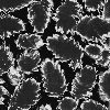
Figure 3: Traditional pipeline for image classification using LBP.

Figure 4: Multi-block LBP with $2\times 2$ non-overlapping blocks.

In the last decade, several variations of the LBP have been proposed to attain different properties. The two best-known variations were proposed by Ojala et. al, the original authors of the LBP methodology: rotation invariant and uniform LBP [5].

Rotation invariance can be achieved by assigning a unique identifier to all the patterns that can be obtained by applying circular shifts. The new encoding is defined in (3), where $ROR(e,i)$ applies a circular-wrapped bit-wise shift of $i$ positions to the encoding $e$.

$$LBP(x_{ref})=\min\{ROR(LBP(x_{ref}),i)\leavevmode\nobreak\ |\leavevmode\nobreak\ i\in[0,\ldots|\cal N|)\}$$ (3)

In the same work, Ojala et. al [5] identified that uniform patterns (i.e. patterns with two or less circular transitions) are responsible for the vast majority of the histogram frequencies, leaving low discriminative power to the remaining ones. Then, the relatively small proportion of non-uniform patterns limits the reliability of their probabilities, all the non-uniform patterns are assigned to a single bin in the histogram construction, while uniform patterns are assigned to individual bins. [5].

Heikkila et. al proposed Center-Symmetric LBP [20], which increases robustness on flat image areas and improves computational efficiency. This is achieved by comparing pairs of neighbors located in centered symmetric directions instead of comparing each neighbor with the reference pixel. Thus, an encoding with four bits is generated from a neighborhood of 8 pixels. Also, the binarization function incorporates an activation tolerance given by $b(x_{i},x_{j})=x_{i}>x_{j}+T$. Further extensions of this idea can be found in [21, 22, 23].

Local ternary patterns (LTP) are an extension of LBP that use a 3-valued mapping instead of a binarization function. The function used by LTP is formalized at (4). LTP are less sensitive to noise in uniform regions at the cost of losing invariance to illumination scaling. Moreover, LTP induce an additional complexity in the number of encodings, producing histograms with up to $3^{\cal N}$ bins.

$$b_{T}(x_{ref},x_{i})=\begin{cases}-1&x_{i}<x_{ref}-T\\ 0&x_{ref}-T\leq x_{i}\leq x_{ref}+T\\ +1&x_{ref}+T<x_{i}\\ \end{cases}$$ (4)

So far, we have mainly described methods that rely on redefining the construction of the LBP encodings. A different line of research focuses on improving LBP by modifying the texture summarization when building the frequency histograms. Two examples of this idea were presented in this work: uniform LBP [5] and multi-block LBP (see Fig. 4).

Since different scales may bring complementary information, one can concatenate the histograms of LBP values at different scales. Berkan et al. proposed this idea in the Over-Complete LBP (OCLBP)[19]. Besides computing the encoding at multiple scales, OCLBP computes the histograms on several spatially overlapped blocks. An alternative to this way of modeling multiscale patterns is to, at each point, compute the LPB code at different scales, concatenate the codes and summarize (i.e., compute the histogram) of the concatenated feature vector. This latter option has difficulties concerning the dimensionality of the data (potentially tackled with a bag of words approach) and the nature of the codes (making unsuitable standard k-means to find the bins-centers for a bag of words approach).

Multi-channel data (e.g. RGB) has been handled in a similar way, by 1) computing and summarizing the LBP codes in each channel independently and then concatenating the histograms [24] and by 2) computing a joint code for the three channels [25].

As LBP have been successfully used to describe spatial relations between pixels, some works explored embedding temporal information on LBP for object detection and background removal [10, 26, 27, 28, 29, 30].

Finally, Local Binary Pattern Network (LBPNet) was introduced by Xi et al. [31] as a preliminary attempt to embed Deep Learning concepts in LBP. Their proposal consists on using a pyramidal approach on the neighborhood scales and histogram sampling. Then, Principal Component Analysis (PCA) is used on the frequency histograms to reduce the dimensionality of the feature space. Xi et al. analogise the pyramidal construction of LBP neighborhoods and histogram sampling as a convolutional layer, where multiple filters operate at different resolutions, and the dimensionality reduction as a Pooling layer. However, LBPNets aren’t capable of aggregating information from a single resolution into higher levels of abstraction which is the main advantage of deep neural networks.

In the next sections, we will bring some ideas from the Deep Learning community to traditional LBP. In this sense, we intend to build LBP blocks that can be applied recursively in order to build features with higher-level of abstraction.

II Deep Local Binary Patterns

The ability to build features with increasing abstraction level using a recursive combination of relatively simple processing modules is one of the reasons that made Convolutional Neural Networks – and in general Neural Networks – so successful. In this work, we propose to represent “higher order” information about texture by applying LBP recursively, i.e., cascading LBP computing blocks one after the other (see Fig 5). In this sense, while an LBP encoding describes the local texture, a second order LBP encoding describes the texture of textures.

Figure 5: Recursive application of Local Binary Patterns.

However, while it is trivial to recursively apply convolutions – and many other filters – in a cascade fashion, traditional LBP are not able to digest their own output.

Traditional LBP rely on receiving as input an image with domain in an ordered set (e.g. grayscale intensities). However, LPB codes are not in an ordered set, dismissing the direct recursive application of standard LBP. As such we will first generalize the main operations supporting LBP and discuss next how to assemble together a deep/recursive LBP feature extractor. We start the discussion with the binarization function $b(x_{ref},x_{i})$.

It is instructive to think, in the conventional LBP, if non-trivial alternative functions exist to the adopted one, Eq. (1). What is(are) the main property(ies) required by the binarization function? Does it need to make use of a (potentially implicit) order relationship? A main property of the binarization function is to be independent of scaling and translation of the input data, that is,

$$b(k_{1}x_{ref}+k_{2},\leavevmode\nobreak\ k_{1}x_{i}+k_{2})=b(x_{ref},x_{i}),\leavevmode\nobreak\ k_{1}>0.$$ (5)

It is trivial to prove that the only options for the binarization function that hold Eq. (5) are the constant functions (always zeros or always ones), the one given by Eq. (1) and its reciprocal.

Proof.

Assume $x_{i},x_{j}>x_{ref}$ and $b(x_{ref},x_{i})\not=b(x_{ref},x_{j})$. Under the independence to translation and scaling (Eq. (5)), $b(x_{ref},x_{i})=b(x_{ref},x_{j})$ as shown below, which is a contradiction.

$$b(x_{ref},x_{i})$$

$$= \left\langle\leavevmode\nobreak\ \text{Identity of multiplication}\leavevmode\nobreak\ \right\rangle$$

$$b\left(\dfrac{x_{j}-x_{ref}}{x_{j}-x_{ref}}x_{ref},\dfrac{x_{j}-x_{ref}}{x_{j}-x_{ref}}x_{i}\right)$$

$$= \left\langle\leavevmode\nobreak\ \text{Identity of addition}\leavevmode\nobreak\ \right\rangle$$

$$b\left(\dfrac{x_{j}-x_{ref}+(x_{i}-x_{i})}{x_{j}-x_{ref}}x_{ref},\dfrac{x_{j}-x_{ref}}{x_{j}-x_{ref}}x_{i}+\left(\dfrac{x_{ref}x_{j}-x_{ref}x_{j}}{x_{j}-x_{ref}}\right)\right)$$

$$= \left\langle\text{Arithmetic}\right\rangle$$

$$b\left(\dfrac{x_{i}-x_{ref}}{x_{j}-x_{ref}}x_{ref}+x_{ref}\dfrac{x_{j}-x_{i}}{x_{j}-x_{ref}},\dfrac{x_{i}-x_{ref}}{x_{j}-x_{ref}}x_{j}+x_{ref}\dfrac{x_{j}-x_{i}}{x_{j}-x_{ref}}\right)$$

$$= \left\langle\leavevmode\nobreak\ \text{Eq.}\leavevmode\nobreak\ \eqref{eq:binproperties}\text{, where}\leavevmode\nobreak\ k_{1}=\dfrac{x_{i}-x_{ref}}{x_{j}-x_{ref}},k_{2}=x_{ref}\dfrac{x_{j}-x_{i}}{x_{j}-x_{ref}}\right\rangle$$

$$b(x_{ref},x_{j})$$

Therefore, $b(x_{ref},x_{i})$ must be equal to all $x_{i}$ above $x_{ref}$. Similarly, $b(x_{ref},x_{i})$ must be equal to all $x_{i}$ below $x_{ref}$. ∎

Among our options, the constant binarization function is not a viable option, since the information (in information theory perspective) in the output is zero. Since the recursive application of functions can be understood as a composition, invariance to scaling and translation is trivially ensured by using a traditional LBP in the first transformation.

Given that transitivity is a relevant property held by the natural ordering of real numbers, we argue that such property should be guaranteed by our binarization function. In this sense, we will focus on strict partial orders of encodings. Following, we show how to build such binarization functions for the i-$th$ application of the LBP operator, where $i>1$. We will consider both predefined/expert driven solutions and data driven solutions (and therefore, application specific).

Hereafter, we will refer to the binarization function as the partial ordering of LBP encodings. Despite the existence of other types of functions may be of general interest, narrowing the search space to those that can be represented as a partial ordering induce efficient learning mechanisms.

II-A Preliminaries

Let us formalize the deep binarization function as the order relation $b^{+}\in{\cal P}(E_{\cal N}\times E_{\cal N})$, where $E_{\cal N}$ is the set of encodings induced by the neighborhood $\cal N$.

Let $\Phi$ be an oracle $\Phi::{\cal P}(E_{\cal N}\times E_{\cal N})\rightarrow\mathbb{R}$ that assesses the performance of a binarization function. For example, among other options, the oracle can be defined as the performance of the traditional LBP pipeline (see Fig. 3) on a dataset for a given predictive task.

II-B Deep Binarization Function

From the entire space of binarization functions, we restrict our analysis to those induced by strict partial orders. Within this context, it is easy to see that learning the best binarization function by exhaustive exploration is intractable since the number of combinations equals the number of directed acyclic graph (DAG) with $2^{|\cal N|}=|E_{\cal N}|$ nodes. The DAG counting problem was studied by Robinson [32] and is given by the recurrence relation Eqs. (6)-(7).

$$a_{0} =1$$ (6)

$$a_{n>1} =\sum\limits_{k=1}^{n}(-1)^{k-1}\binom{n}{k}2^{k(n-k)}a_{n-k}$$ (7)

Table I: Lower bound of the number of combinations for deciding the best LBP binarization function as partial orders.

# Neighbors	Rotational Inv.	Uniform	Traditional
$2$	$2\cdot 10^{1}$	$2\cdot 10^{4}$	$5\cdot 10^{2}$
$3$	$5\cdot 10^{2}$	$1\cdot 10^{15}$	$7\cdot 10^{11}$
$4$	$3\cdot 10^{6}$	$2\cdot 10^{41}$	$8\cdot 10^{46}$
$5$	$7\cdot 10^{11}$	$6\cdot 10^{94}$	$2\cdot 10^{179}$
$6$	$1\cdot 10^{36}$	$2\cdot 10^{190}$	$1\cdot 10^{685}$
$7$	$2\cdot 10^{72}$	$3\cdot 10^{346}$	$3\cdot 10^{2640}$
$8$	$1\cdot 10^{225}$	$1\cdot 10^{585}$	$3\cdot 10^{10288}$

Table I illustrates the size of the search space for several numbers of neighbors. For instance, for the traditional setting with 8 neighbors, the number of combinations has more than 10,000 digits. Thereby, a heuristic approximation must be carried out.

II-B1 Learning $b^{+}$ from a User-defined dissimilarity function

The definition of a dissimilarity function between two codes seems reasonably accessible. For instance, an immediate option is to adopt the hamming distance between codes, $d_{H}$. With rotation invariance in mind, one can adopt the minimum hamming distance between all circularly shifted versions of $x_{ref}$ and $x_{i}$, $d_{H}^{ri}$. The circular invariant hamming distance between $x_{ref}$ and $x_{i}$ can be computed as

$$d_{H}^{ri}=\min\limits_{s\in{0,\cdots,{\cal N}-1}}d_{H}(ROR(x_{ref},s),x_{i})$$ (8)

Having defined such a dissimilarity function between pairs of codes, one can know proceed with the definition of the binarization function.

Given the dissimilarity function, we can learn a mapping of the codes to an ordered set. Resorting to Spectral Embedding [33], one can obtain such a mapping. The conventional binarization function, Eq. (1), can then be applied. Other alternatives for building the mappings can be found in the manifold learning literature: Isomaps [34], Multidimensional scaling (MDS) [35], among others. In this case, the oracle function can be defined as the intrinsic loss functions used in the optimization process of such algorithms.

Preserving a desired property $P$ such as rotational invariance and sign invariance (i.e. interchangeability between ones and zeros) can be achieved by considering $P$-aware dissimilarities.

II-B2 Learning $b^{+}$ from a High-dimensional Space

A second option is to map the code space to a new (higher-dimensional) space that characterizes LBP encodings. Then, an ordering or preference relationship can be learned in the extended space, for instance resorting to preference learning algorithms [36, 37, 38].

Some examples of properties that characterize LBP encodings are:

• Number of transitions of size 1 (e.g. 101, 010).

• Number of groups/transitions.

• Size of the smallest/largest group.

• Diversity on the group sizes.

• Number of ones.

Techniques to learn the final ordering based on the new high-dimensional space include:

• Dimensionality reduction techniques, including Spectral embeddings, PCA, MDS and other manifold techniques.

• Preference learning strategies for learning rankings [36, 37, 38].

A case of special interest that will be used in the experimental section of this work are Lexicographic Rankers (LR) [38, 36]. In this work, we will focus on the simplest type of LR, linear LR. Let us assume that features in the new high-dimensional space are scoring rankers (e.g. monotonic functions) on the texture complexity of the codes. Thus, for each code $e_{i}$ and feature $s_{j}$, the complexity associated to $e_{i}$ by $s_{j}$ is denoted as $s_{j}(e_{i})$. We assume $s_{j}(e_{i})$ to lie in a discrete domain with a well-known order relation.

Thus, each feature is grouping the codes into equivalence classes. For example, the codes with 0 transitions (i.e. flat textures), 2 transitions (i.e. uniform textures) and so on.

If we concatenate the output of the scoring rankers in a linear manner $(s_{0}(e_{i}),s_{1}(e_{i}),\cdots,s_{n}(e_{i}))$, a natural arrangement is their lexicographic order (see Eq. (9)), where each $s_{j}(e_{i})$ is subordering the equivalence class obtained by the previous prefix of rankers $(s_{0}(e_{i}),\cdots,s_{j-1}(e_{i}))$.

$$\text{LexRank}(a,b)=\begin{cases}a=b&,|a|=0\leavevmode\nobreak\ \vee|b|=0\\ a\prec b&,a_{0}\prec b_{0}\\ a\succ b&,a_{0}\succ b_{0}\\ LexRank(t(a),t(b))&,a_{0}=b_{0}\\ \end{cases}$$ (9)

where $t(a)$ returns the tail of the sequence. Namely, the order between two encodings is decided by the first scoring ranker in the hierarchy that assigns different values to the encodings.

Therefore, the learning process is reduced to find the best feature arrangement. A heuristic approximation to this problem can be achieved by iteratively appending to the sequence of features the one that maximizes the performance of the oracle $\Phi$.

Similarly to property-aware dissimilarity functions, if the features in the new feature vector ${\cal V}(x)$ are invariant to $P$, the $P$-invariance of the learned binarization function is automatically guaranteed.

III Deep Architectures

Given the closed form of the LBP with deep binarization functions, their recursive combination seems feasible. In this section, several alternatives for the aggregation of deep LBP operators are proposed.

III-A Deep LBP (DLBP)

Figure 6: Deep LBP.

The simplest way of aggregating Deep LBP operators is by applying them recursively and computing the final encoding histograms. Figure 6 shows this architecture. The first transformation is done by a traditional shallow LBP while the remaining transformations are performed using deep binarization functions.

Figure 7 illustrates the patterns detected by several deep levels on a cracker image from the Brodatz database. In this case, the ordering between LBP encodings was learned by using a lexicographic ordering of encodings on the number of groups, the size of the largest group and imbalance ratio between 0’s and 1’s. We can observe that the initial layers of the architecture extract information from local textures while the later layers have higher levels of abstraction.

(a) Input image

(b) LBP

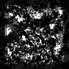
(c) DeepLBP(1)

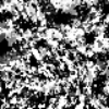
(d) DeepLBP(2)

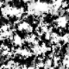
(e) DeepLBP(3)

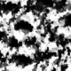
(f) DeepLBP(4)

Figure 7: Visualization of LBP encodings from a Brodatz database [39] image. The results obtained by applying n layers of Deep LBP operators are denoted as DeepLBP(n). A neighborhood of size 8, radius 10 and Euclidean distance was used. The grayscale intensity is defined by the order of the equivalence classes.

III-B Multi-Deep LBP (MDLBP)

Despite it may be a good idea to extract higher-order information from images, for the usual applications of LBP, it is important to be able to detect features at different levels of abstraction. For instance, if the image has textures with several complexity levels, it may be relevant to keep the patterns extracted at different abstraction levels. Resorting to the techniques employed in the analysis of multimodal data [40], we can aggregate this information in two ways: feature and decision-level fusion.

III-B1 Feature-level fusion

one histogram is computed at each layer and the model is built using the concatenation of all the histograms as features.

III-B2 Decision-level fusion

one histogram and decision model is computed at each layer. The final model uses the probabilities estimated by each individual model to produce the final decision.

Figures 8(a) and 8(b) show Multi-Deep LBP architectures with feature-level and decision-level fusion respectively. In our experimental setting, feature-level fusion was used.

(a) Multi-Deep LBP with feature-level fusion.

(b) Multi-Deep LBP with decision-level fusion.

Figure 8: Deep LBP architectures.

III-C Multiscale Deep LBP (Multiscale DLBP)

Figure 9: Multi-scale Deep LBP.

In the last few years, deep learning approaches have benefited from multi-scale architectures that are able to aggregate information from different image scales [41, 42, 43]. Despite being able to induce higher abstraction levels, deep networks are restrained to the size of the individual operators. Thereby, aggregating multi-scale information in deep architectures may exploit their capability to detect traits that appear at different scales in the images in addition to turning the decision process scale invariant.

In this work, we consider the stacking of independent deep architectures at several scales. The final decision is done by concatenating the individual information produced at each scale factor (cf. Figure 9). Depending on the fusion approach, the final model operates in different spaces (i.e. feature or decision level). In an LBP context, we can define the scale operator of an image by resizing the image or by increasing the neighborhood radius.

IV Experiments

Table II: Summary of the datasets used in the experiments

Dataset	Reference	Task	Images	Classes
KTH TIPS	[44]	Texture	810	10
FMD	[45]	Texture	1000	10
Virus	[46]	Texture	1500	15
Brodatz*	[39]	Texture	1776	111
Kylberg	[47]	Texture	4480	28
102 Flowers	[48]	Object	8189	102
Caltech 101	[49]	Object	9144	102

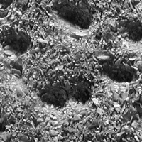
(a) KTH TIPS

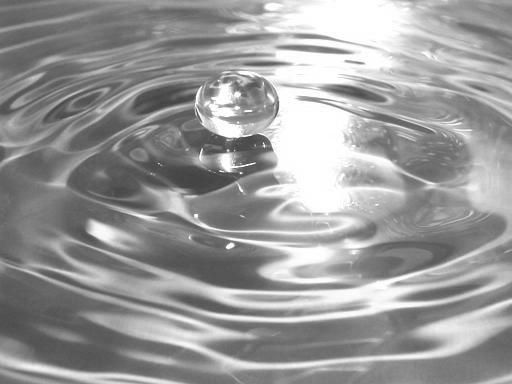
(b) FMD

(c) Virus

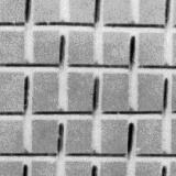
(d) Brodatz

(e) Kylberg

(f) 102 Flowers

(g) Caltech 101

Figure 10: Sample images from each dataset

In this section, we compare the performance of the proposed deep LBP architectures against shallow LBP versions. Several datasets were chosen from the LBP literature covering a wide range of applications, from texture categorization to object recognition. Table II summarizes the datasets used in this work. Also, Fig. 10 shows an image per dataset in order to understand the task diversity.

We used a 10-fold stratified cross-validation strategy and the average performance of each method was measured in terms of:

• Accuracy.

• Class rank: Position (%) of the ground truth label in the ranking of classes ordered by confidence. The ranking was induced using probabilistic classifiers.

While high values are preferred when using accuracy, low values are preferred for class rank. All the images were resized to have a maximum size of $100\times 100$ and the neighborhood used for all the LBP operators was formed by 8 neighbors on a radius of size 3, which proved to be a good configuration for the baseline LBP. The final features were built using a global histogram, without resorting to image blocks. Further improvements in each application can be achieved by fine-tuning the LBP neighborhoods and by using other spatial sampling techniques on the histogram construction. Since the objective of this work was to objectively compare the performance of each strategy, we decided to fix these parameters. The final decision model is a Random Forest with 1000 trees. In the last two datasets, which contain more than 100 classes, the maximum depth of the decision trees was bounded to 20 in order to limit the required memory.

In all our experiments, training data was augmented by including vertical and horizontal flips.

Table III: Class rank (%) of the ground-truth label and accuracy with single-scale strategies

Dataset	Strategy	Class Rank					Accuracy
		Layers					Layers
		1	2	3	4	5	1	2	3	4	5
	Similarity	-	19.18	18.87	18.26	18.80	-	53.28	53.28	53.28	53.28
	High Dim	-	18.64	18.78	18.79	19.10	-	53.28	53.28	53.28	53.28
KTH TIPS	LBP	1.55	-	-	-	-	89.22	-	-	-	-
	Similarity	-	1.60	1.68	1.82	1.86	-	88.96	88.57	86.99	87.97
	High Dim	-	0.94	0.91	1.09	1.11	-	92.96	93.58	92.72	92.36
FMD	LBP	26.96	-	-	-	-	29.20	-	-	-	-
	Similarity	-	25.77	25.79	25.61	25.59	-	28.90	30.00	30.90	30.80
	High Dim	-	23.20	23.36	23.30	23.50	-	33.40	32.60	33.30	33.00
Virus	LBP	8.08	-	-	-	-	56.80	-	-	-	-
	Similarity	-	6.61	6.78	6.72	6.73	-	61.00	61.33	60.93	61.93
	High Dim	-	6.65	6.50	6.53	6.55	-	61.53	61.27	61.47	62.27
Brodatz	LBP	0.25	-	-	-	-	89.23	-	-	-	-
	Similarity	-	0.22	0.22	0.23	0.25	-	89.73	90.23	90.50	90.36
	High Dim	-	0.21	0.21	0.22	0.23	-	90.72	90.72	90.09	89.59
Kylberg	LBP	0.23	-	-	-	-	95.29	-	-	-	-
	Similarity	-	0.18	0.16	0.14	0.14	-	96.14	96.52	96.72	96.81
	High Dim	-	0.07	0.07	0.07	0.07	-	98.37	98.35	98.26	98.24
102 Flowers	LBP	13.46	-	-	-	-	23.18	-	-	-	-
	Similarity	-	13.34	13.56	13.99	14.29	-	25.59	24.46	24.92	24.58
	High Dim	-	13.10	12.99	13.15	13.32	-	24.56	23.76	22.81	22.36
Caltech 101	LBP	13.05	-	-	-	-	39.71	-	-	-	-
	Similarity	-	12.37	12.23	12.32	12.38	-	40.35	40.07	39.74	39.81
	High Dim	-	11.98	12.19	12.16	12.34	-	41.45	40.78	40.56	40.43

IV-A Single-scale

First, we validated the performance of the proposed deep architectures on single scale settings with increasing number of deep layers. Information from each layer was merged at a feature level by concatenating the layerwise histogram (c.f. Section III-B). Table III summarizes the results of this setting. In all the datasets, the proposed models surpassed the results achieved by traditional LBP.

Furthermore, even when the accuracy gains are small, the large gains in terms of class rank suggest that the deep architectures induce more stable models, which assign a high probability on the ground-truth level, even on misclassified cases. For instance, in the Kylberg dataset, a small relative accuracy gain of 3.23% was achieved by the High Dimensional rule, the relative gain on the class rank was 69.56%.

With a few exceptions (e.g. JAFFE dataset), the data-driven deep operator based on a high dimensional projection achieved the best performance. Despite the possibility to induce encoding orderings using user-defined similarity functions, the final orderings are static and domain independent. In this sense, more flexible data-driven approaches as the one suggested in Section II-B2 are able to take advantage of the dataset-specific properties.

Despite the capability of the proposed deep architectures to achieve large gain margins, the deep LBP operators saturate rapidly. For instance, most of the best results were found on architectures with up to three deep layers. Further research on aggregation techniques to achieve higher levels of abstraction should be conducted. For instance, it would be interesting to explore efficient non-parametric approaches for building encoding orderings that allow more flexible data-driven optimization.

IV-B Multi-Scale

A relevant question in this context is if the observed gains are due to the higher abstraction levels of the deep LBP encodings or to the aggregation of information from larger neighborhoods. Namely, when applying a second order operator, the neighbors of the reference pixel include information from their own neighborhood which was initially out of the scope of the local LBP operator. Thereby, we compare the performance of the Deep LBP and multiscale LBP.

In order to simplify the model assessment, we fixed the number of layers to 3 in the deep architectures. A scaling factor of 0.5 was used on each layer of the pyramidal multiscale operator. Guided by the results achieved in the single-scale experiments, the deep operator based on the lexicographic sorting of the high-dimensional feature space was used in all cases.

Table IV summarizes the results on the multiscale settings. In most cases, all the deep LBP architectures surpassed the performance of the best multiscale shallow architecture. Thereby, the aggregation level achieved by deep LBP operators goes beyond a multiscale analysis, being able to address meta-texture information. Furthermore, when combined with a multiscale approach, deep LBP achieved the best results in all the cases.

Table IV: Class rank (%) of the ground-truth label and accuracy with multi-scale strategies

Dataset	Strategy	Class Rank			Accuracy
		Scales			Scales
		1	2	3	1	2	3
KTH TIPS	Shallow	1.55	1.17	1.22	89.22	90.94	90.93
	Deep	0.91	0.79	0.62	93.58	94.21	94.96
FMD	Shallow	26.96	26.31	26.32	29.20	29.60	29.80
	Deep	23.36	23.54	23.77	32.60	33.20	33.00
Virus	Shallow	8.08	7.51	7.97	56.80	60.60	58.60
	Deep	6.50	5.92	6.04	61.27	66.13	64.87
Brodatz	Shallow	0.25	0.20	0.23	89.23	90.77	90.00
	Deep	0.21	0.13	0.13	90.72	92.97	93.11
Kylberg	Shallow	0.23	0.13	0.12	95.29	97.34	97.57
	Deep	0.07	0.05	0.04	98.35	98.84	98.95
102 Flowers	Shallow	13.46	13.10	12.79	23.18	25.10	26.40
	Deep	12.99	12.68	12.71	23.76	26.02	26.87
Caltech 101	Shallow	12.92	12.46	12.28	40.07	40.84	41.03
	Deep	12.21	11.74	11.60	40.68	41.67	42.01

IV-C LBPNet

Finally, we compare the performance of our deep LBP architecture against the state of the art LBPNet [31]. As referred in the introduction, LBPNet uses LBP encodings at different neighborhood radius and histogram sampling in order to simulate the process of learning a bag of convolutional filters in deep networks. Then, the dimensionality of the descriptors are reduced by means of PCA, resorting to the idea of pooling layers from Convolutional Neural Networks (CNN). However, the output of a LBPNet cannot be used by itself in successive calls of the same function. Thereby, it is uncapable of building features with higher expresiveness than the individual operators.

In our experiments, we considered the best LBPNet with up to three scales and histogram computations with nonoverlapping histograms that divide the image in $1\times 1$, $2\times 2$ and $3\times 3$ blocks. The number of components kept in the PCA transformation was chosen in order to retain 95% of the variance for most datasets with the exception of 102 Flowers and Caltech, where a value of 99% was chosen due to poor performance of the previous value. A global histogram was used in our deep LBP architecture

Table V summarizes the results obtained by multiscale LBP (shallow), LBPNet and our proposed deep LBP. In order to understand if the gains achieved by the LBPNet are due to the overcomplete sampling or to the PCA transformation preceeding the final classifier, we validated the performance of our deep architecture with a PCA transformation on the global descriptor before applying the Random Forest classifier. Despite being able to surpass the performance of our deep LBP without dimensionality reduction, LBPNet did not improve the results obtained by our deep architecture with PCA in most cases. In this sense, even whithout resorting to local descriptors on the histogram sampling, our model was able to achieve the best results within the family of LBP methods. The only exception was observed in the 102 Flowers dataset (see Fig. 10(f)), where the spatial information can be relevant. It is important to note that our model can also benefit from using spatial sampling of the LBP activations. Moreover, deep learning concepts such as dropout and pooling layers can be introduced within the Deep LBP architectures in a straightforward manner.

Table V: Class rank (%) of the ground-truth label and accuracy

Dataset	Strategy	Class Rank	Accuracy
KTH TIPS	Shallow	1.17	90.94
	LBPNet	0.43	96.29
	Deep LBP	0.62	94.96
	Deep LBP (PCA)	0.16	98.39
FMD	Shallow	26.31	29.80
	LBPNet	25.71	30.00
	Deep LBP	23.36	33.20
	Deep LBP (PCA)	23.20	32.30
Virus	Shallow	7.51	60.60
	LBPNet	7.18	60.73
	Deep LBP	5.92	66.13
	Deep LBP (PCA)	5.91	65.60
Brodatz	Shallow	0.20	90.77
	LBPNet	0.20	91.49
	Deep LBP	0.13	93.11
	Deep LBP (PCA)	0.12	94.46
Kylberg	Shallow	0.12	97.57
	LBPNet	0.19	95.80
	Deep LBP	0.04	98.95
	Deep LBP (PCA)	0.02	99.55
102 Flowers	Shallow	12.79	26.40
	LBPNet	9.61	35.56
	Deep LBP	12.68	26.87
	Deep LBP (PCA)	22.30	8.80
Caltech 101	Shallow	12.46	41.03
	LBPNet	12.11	42.69
	Deep LBP	11.60	42.01
	Deep LBP (PCA)	10.87	45.14

V Conclusions

Local Binary Patterns have achieved competitive performance in several computer vision tasks, being a robust and easy to compute descriptor with high discriminative power on a wide spectrum of tasks. In this work, we proposed Deep Local Binary Patterns, an extension of the traditional LBP that allow successive applications of the operator. By applying LBP in a recursive way, features with higher level of abstraction are computed that improve the descriptor discriminability.

The key aspect of our proposal is the introduction of flexible binarization rules that define an order relation between LBP encodings. This was achieved with two main learning paradigms. First, learning the ordering based on a user-defined encoding similarity metric. Second, allowing the user to describe LBP encodings on a high-dimensional space and learning the ordering on the extended space directly. Both ideas improved the performance of traditional LBP in a diverse set of datasets, covering various applications such as face analysis, texture categorization and object detection. As expected, the paradigm based on a projection to a high-dimensional space achieved the best performance, given its capability of using application specific knowledge in an efficient way. The proposed deep LBP are able to aggregate information from local neighborhoods into higher abstraction levels, being able to surpass the performance obtained by multiscale LBP as well.

While the advantages of the proposed approach were demonstrated in the experimental section, further research can be conducted on several areas. For instance, it would be interesting to find the minimal properties of interest that should be guaranteed by the binarization function. In this work, since we are dealing with intensity-based image, we restricted our analysis to partial orderings. However, under the presence of other types of data such as directional (i.e. periodic, angular) data, cycling or local orderings could be more suitable. In the most extreme case, the binarization function may be arbitrarily complex without being restricted to strict orders.

On the other hand, constraining the shape of the binarization function allows more efficient ways to find suitable candidates. In this sense, it is relevant to explore ways to improve the performance of the similarity-based deep LBP. Two possible options would be to refine the final embedding by using training data and allowing the user to specify incomplete similarity information.

In this work, each layer was learned in a local fashion, without space for further refinement. While this idea was commonly used in the deep learning community when training stacked networks, later improvements take advantage of refining locally trained architectures [50]. Therefore, we plan to explore global optimization techniques to refine the layerwise binarization functions.

Deep learning imposed a new era in computer vision and machine learning, achieving outstanding results on applications where previous state-of-the-art methods performed poorly. While the foundations of deep learning rely on very simple image processing operators, relevant properties held by traditional methods, such as illumination and rotational invariance, are not guaranteed. Moreover, the amount of data required to learn competitive deep models from scratch is usually prohibitive. Thereby, it is relevant to explore the path into a unification of traditional and deep learning concepts. In this work, we explored this idea within the context of Local Binary Patterns. The extension of deep concepts to other traditional methods is of great interest in order to rekindle the most fundamental concepts of computer vision to the research community.

References

- [1] J. Xie, L. Xu, and E. Chen, “Image denoising and inpainting with deep neural networks,” in Advances in Neural Information Processing Systems, 2012, pp. 341–349.
- [2] B. Zhou, A. Lapedriza, J. Xiao, A. Torralba, and A. Oliva, “Learning deep features for scene recognition using places database,” in Advances in neural information processing systems, 2014, pp. 487–495.
- [3] Y. Cho and L. K. Saul, “Kernel methods for deep learning,” in Advances in neural information processing systems, 2009, pp. 342–350.
- [4] T. Ojala, M. Pietikäinen, and T. Mäenpää, “Gray scale and rotation invariant texture classification with local binary patterns,” in European Conference on Computer Vision. Springer, 2000, pp. 404–420.
- [5] T. Ojala, M. Pietikainen, and T. Maenpaa, “Multiresolution gray-scale and rotation invariant texture classification with local binary patterns,” IEEE Transactions on pattern analysis and machine intelligence, vol. 24, no. 7, pp. 971–987, 2002.
- [6] L. Liu, L. Zhao, Y. Long, G. Kuang, and P. Fieguth, “Extended local binary patterns for texture classification,” Image and Vision Computing, vol. 30, no. 2, pp. 86–99, 2012.
- [7] Y. Zhao, W. Jia, R.-X. Hu, and H. Min, “Completed robust local binary pattern for texture classification,” Neurocomputing, vol. 106, pp. 68–76, 2013.
- [8] Z. Guo, L. Zhang, and D. Zhang, “Rotation invariant texture classification using lbp variance (lbpv) with global matching,” Pattern recognition, vol. 43, no. 3, pp. 706–719, 2010.
- [9] ——, “A completed modeling of local binary pattern operator for texture classification,” IEEE Transactions on Image Processing, vol. 19, no. 6, pp. 1657–1663, 2010.
- [10] G. Zhao and M. Pietikainen, “Dynamic texture recognition using local binary patterns with an application to facial expressions,” IEEE transactions on pattern analysis and machine intelligence, vol. 29, no. 6, 2007.
- [11] T. Ahonen, A. Hadid, and M. Pietikäinen, “Face recognition with local binary patterns,” in European conference on computer vision. Springer, 2004, pp. 469–481.
- [12] B. Zhang, Y. Gao, S. Zhao, and J. Liu, “Local derivative pattern versus local binary pattern: face recognition with high-order local pattern descriptor,” IEEE transactions on image processing, vol. 19, no. 2, pp. 533–544, 2010.
- [13] J. Ren, X. Jiang, and J. Yuan, “Noise-resistant local binary pattern with an embedded error-correction mechanism,” IEEE Transactions on Image Processing, vol. 22, no. 10, pp. 4049–4060, 2013.
- [14] C. Shan, “Learning local binary patterns for gender classification on real-world face images,” Pattern Recognition Letters, vol. 33, no. 4, pp. 431–437, 2012.
- [15] D. Huang, C. Shan, M. Ardabilian, Y. Wang, and L. Chen, “Local binary patterns and its application to facial image analysis: a survey,” IEEE Transactions on Systems, Man, and Cybernetics, Part C (Applications and Reviews), vol. 41, no. 6, pp. 765–781, 2011.
- [16] L. Yeffet and L. Wolf, “Local trinary patterns for human action recognition,” in Computer Vision, 2009 IEEE 12th International Conference on. IEEE, 2009, pp. 492–497.
- [17] L. Nanni, A. Lumini, and S. Brahnam, “Local binary patterns variants as texture descriptors for medical image analysis,” Artificial intelligence in medicine, vol. 49, no. 2, pp. 117–125, 2010.
- [18] T. Xu, E. Kim, and X. Huang, “Adjustable adaboost classifier and pyramid features for image-based cervical cancer diagnosis,” in Biomedical Imaging (ISBI), 2015 IEEE 12th International Symposium on. IEEE, 2015, pp. 281–285.
- [19] O. Barkan, J. Weill, L. Wolf, and H. Aronowitz, “Fast high dimensional vector multiplication face recognition,” in Proceedings of the IEEE International Conference on Computer Vision, 2013, pp. 1960–1967.
- [20] M. Heikkilä, M. Pietikäinen, and C. Schmid, “Description of interest regions with center-symmetric local binary patterns,” in Computer vision, graphics and image processing. Springer, 2006, pp. 58–69.
- [21] J. Trefnỳ and J. Matas, “Extended set of local binary patterns for rapid object detection,” in Computer Vision Winter Workshop, 2010, pp. 1–7.
- [22] G. Xue, L. Song, J. Sun, and M. Wu, “Hybrid center-symmetric local pattern for dynamic background subtraction,” in Multimedia and Expo (ICME), 2011 IEEE International Conference on. IEEE, 2011, pp. 1–6.
- [23] C. Silva, T. Bouwmans, and C. Frélicot, “An extended center-symmetric local binary pattern for background modeling and subtraction in videos,” in International Joint Conference on Computer Vision, Imaging and Computer Graphics Theory and Applications, VISAPP 2015, 2015.
- [24] J. Y. Choi, K. N. Plataniotis, and Y. M. Ro, “Using colour local binary pattern features for face recognition,” in Image Processing (ICIP), 2010 17th IEEE International Conference on. IEEE, 2010, pp. 4541–4544.
- [25] C. Zhu, C.-E. Bichot, and L. Chen, “Multi-scale color local binary patterns for visual object classes recognition,” in Pattern Recognition (ICPR), 2010 20th International Conference on. IEEE, 2010, pp. 3065–3068.
- [26] S. Zhang, H. Yao, and S. Liu, “Dynamic background modeling and subtraction using spatio-temporal local binary patterns,” in Image Processing, 2008. ICIP 2008. 15th IEEE International Conference on. IEEE, 2008, pp. 1556–1559.
- [27] G. Xue, J. Sun, and L. Song, “Dynamic background subtraction based on spatial extended center-symmetric local binary pattern,” in Multimedia and Expo (ICME), 2010 IEEE International Conference on. IEEE, 2010, pp. 1050–1054.
- [28] J. Yang, S. Wang, Z. Lei, Y. Zhao, and S. Z. Li, “Spatio-temporal lbp based moving object segmentation in compressed domain,” in Advanced Video and Signal-Based Surveillance (AVSS), 2012 IEEE Ninth International Conference on. IEEE, 2012, pp. 252–257.
- [29] H. Yin, H. Yang, H. Su, and C. Zhang, “Dynamic background subtraction based on appearance and motion pattern,” in Multimedia and Expo Workshops (ICMEW), 2013 IEEE International Conference on. IEEE, 2013, pp. 1–6.
- [30] S. H. Davarpanah, F. Khalid, L. N. Abdullah, and M. Golchin, “A texture descriptor: Background local binary pattern (bglbp),” Multimedia Tools and Applications, vol. 75, no. 11, pp. 6549–6568, 2016.
- [31] M. Xi, L. Chen, D. Polajnar, and W. Tong, “Local binary pattern network: a deep learning approach for face recognition,” in Image Processing (ICIP), 2016 IEEE International Conference on. IEEE, 2016, pp. 3224–3228.
- [32] R. W. Robinson, “Counting unlabeled acyclic digraphs,” in Combinatorial mathematics V. Springer, 1977, pp. 28–43.
- [33] A. Y. Ng, M. I. Jordan, Y. Weiss et al., “On spectral clustering: Analysis and an algorithm,” in NIPS, vol. 14, no. 2, 2001, pp. 849–856.
- [34] J. B. Tenenbaum, V. De Silva, and J. C. Langford, “A global geometric framework for nonlinear dimensionality reduction,” science, vol. 290, no. 5500, pp. 2319–2323, 2000.
- [35] J. B. Kruskal, “Nonmetric multidimensional scaling: a numerical method,” Psychometrika, vol. 29, no. 2, pp. 115–129, 1964.
- [36] K. Fernandes, J. S. Cardoso, and H. Palacios, “Learning and ensembling lexicographic preference trees with multiple kernels,” in Neural Networks (IJCNN), 2016 International Joint Conference on. IEEE, 2016, pp. 2140–2147.
- [37] T. Joachims, “Optimizing search engines using clickthrough data,” in Proceedings of the eighth ACM SIGKDD international conference on Knowledge discovery and data mining. ACM, 2002, pp. 133–142.
- [38] P. Flach and E. T. Matsubara, “A simple lexicographic ranker and probability estimator,” in European Conference on Machine Learning. Springer, 2007, pp. 575–582.
- [39] P. Brodatz, Textures: a photographic album for artists and designers. Dover Pubns, 1966.
- [40] A. Kapoor and R. W. Picard, “Multimodal affect recognition in learning environments,” in Proceedings of the 13th annual ACM international conference on Multimedia. ACM, 2005, pp. 677–682.
- [41] D. Eigen, C. Puhrsch, and R. Fergus, “Depth map prediction from a single image using a multi-scale deep network,” in Advances in neural information processing systems, 2014, pp. 2366–2374.
- [42] N. Neverova, C. Wolf, G. W. Taylor, and F. Nebout, “Multi-scale deep learning for gesture detection and localization,” in Workshop at the European Conference on Computer Vision. Springer, 2014, pp. 474–490.
- [43] J. Wang, Y. Song, T. Leung, C. Rosenberg, J. Wang, J. Philbin, B. Chen, and Y. Wu, “Learning fine-grained image similarity with deep ranking,” in Proceedings of the IEEE Conference on Computer Vision and Pattern Recognition, 2014, pp. 1386–1393.
- [44] E. Hayman, B. Caputo, M. Fritz, and J.-O. Eklundh, “On the significance of real-world conditions for material classification,” in European conference on computer vision. Springer, 2004, pp. 253–266.
- [45] L. Sharan, R. Rosenholtz, and E. Adelson, “Material perception: What can you see in a brief glance?” Journal of Vision, vol. 9, no. 8, pp. 784–784, 2009.
- [46] C. San Martin and S.-W. Kim, Eds., Virus Texture Analysis Using Local Binary Patterns and Radial Density Profiles, ser. Lecture Notes in Computer Science, vol. 7042. Springer Berlin / Heidelberg, 2011.
- [47] G. Kylberg, “The kylberg texture dataset v. 1.0,” Centre for Image Analysis, Swedish University of Agricultural Sciences and Uppsala University, Uppsala, Sweden, External report (Blue series) 35, September 2011. [Online]. Available: http://www.cb.uu.se/ gustaf/texture/
- [48] M.-E. Nilsback and A. Zisserman, “Automated flower classification over a large number of classes,” in Proceedings of the Indian Conference on Computer Vision, Graphics and Image Processing, Dec 2008.
- [49] L. Fei-Fei, R. Fergus, and P. Perona, “One-shot learning of object categories,” IEEE transactions on pattern analysis and machine intelligence, vol. 28, no. 4, pp. 594–611, 2006.
- [50] M. Norouzi, M. Ranjbar, and G. Mori, “Stacks of convolutional restricted boltzmann machines for shift-invariant feature learning,” in Computer Vision and Pattern Recognition, 2009. CVPR 2009. IEEE Conference on. IEEE, 2009, pp. 2735–2742.