Metric Map Merging using RFID Tags & Topological Information

Abstract

A map merging component is crucial for the proper functionality of a multi-robot system performing exploration, since it provides the means to integrate and distribute the most important information carried by the agents: the explored/covered space and its exact (depending on the SLAM accuracy) morphology. Map merging is a prerequisite for an intelligent multi-robot team aiming to deploy a smart exploration technique. In the current work, a metric map merging approach based on environmental information is proposed, in conjunction with spatially scattered RFID tags localization. This approach is divided into the following parts: the maps’ approximate rotation calculation via the obstacles’ poses and localized RFID tags, the translation employing the best localized common RFID tag and finally the transformation refinement using an ICP algorithm.

1 Introduction

One of the most promising aspects of rescue robotics is the employment of multiple robots to simultaneously operate in a disaster afflicted environment. A robotic team’s deployment presents significant benefits compared to single agent approaches. First of all, the overall performance is boosted as larger areas are explored and covered per time unit, due to the robots’ distributed operation. Next, a multi-agent system is more robust, as the exploration may resume even after a potential robot failure. Finally, the deployment of many identical or heterogeneous robots vastly reduces such a system’s cost, as a single robot equipped with expensive sensors can be replaced with an ensemble of cheap vehicles with limited sensing capabilities.

In order for multiple robots to achieve efficient cooperation, a mechanism should exist to support the sharing of their distributed information. Even if they are able to flawlessly communicate with each other, it is impossible to properly merge specific parts of information, i.e. map representations, without the existence of a common reference. In the simplest case, common reference refers to a two dimensional transformation between the robotic agents’ local coordinate systems. Thus, it is understandable that the aforementioned transformation should be efficiently calculated in order for true group intelligence to exist.

In the current work, the map representation used is OGM (occupancy grid map). OGMs are metric depictions of the environment, consisting of a grid of cells, each of which is assigned an occupancy probability value. A specific cell’s occupancy probability is altered according to the current range sensors’ measurements. Our main focus is to create an efficient approach towards merging local OGMs using topological information and RFID tags, by dividing the problem into the calculation of the translation and rotation separately. Our proposal consists of several consecutive steps. The first step is to accurately compute an alignment angle concerning the environmental obstacles, which we assume to be orthogonal. Next, the correct rotation quaternion is determined via the topological alignment of common RFID tags’ poses among the robots. The third step implements the translation calculation employing the best localized pair of RFID tags. These steps can achieve a quite good approximation of the actual transformation. However, in order to achieve an exact alignment, an additional step is introduced, including the deployment of an ICP (Iterative Closest Point) algorithm. Finally, due to the discrete map representation, inconsistencies appear after the transformation’s application. This issue is resolved using a modified blurring process.

The paper is organized as follows. In section 2 the State of the Art concerning the map merging problem is presented. Section 3 describes the RFID tag localization procedure and section 4 contains the actual steps of the map merging implementation. In section 5 the experiments are presented and finally in section 6 conclusions and future work are discussed.

2 Related Work

In [1], Carpin and Birk suggest a quite straightforward map merging method. The proposed solution implements a stochastic search in the map transformations space, comprised of translations and rotations. This search method consists of a time variant Gaussian Random Walk, altering its distribution parameters in order to employ its recent values’ history, approaching the correct solution.

A different method is presented in [2], where the data association problem is resolved using wireless sensors’ IDs, detectable by an omnidirectional 2.4 GHz antenna. These are employed for a map merging common reference frame calculation. Each robot submits its pose in the wireless sensor memory, allowing robots to acknowledge that they share a common explored area. A similar approach is followed in the current work, suggesting the use of spatially scattered RFID tags, whose pose is probabilistically localized and, if special conditions are met, map merging is performed. In our approach we experimentally prove that without the exact wireless sensors’ pose it is impossible to achieve precise map merging, thus extra optimization methods are required. The original probabilistic technique for the RFID tags’ pose calculation using Bayes filters is presented in [3]. A two dimensional probability distribution of a single tag is calculated, based on the actual RFID antenna and reader operating field, whilst in our case an ideal uniform omnidirectional antenna was assumed.

In [4], Konolige, Fox et al., suggest a distributed mapping technique under uncertain communication, as well as an algorithm for the robot poses localization in the local maps. Specifically, the $i^{th}$ robot’s pose in the $j^{th}$ robot’s local map, is calculated by using a small fraction of $i$’s map, in which three distinct topological features are recognized: corners, doors and junctions. Next, following a similar procedure in $j$’s map and by utilizing probabilistic methods, the dominant $i$’s pose is calculated, enabling the information exchange.

Following a similar approach incorporating features, Amigoni and Gasparini suggest a map merging method with no odometry information requirements in [5]. This allows for map merging just from the map representations, providing flexibility to the algorithm. In this publication, the features are corners resulting from the straight line segments which form the environmental obstacles. The merging procedure consists of three steps: a) the creation of possible transformations based on feature matching, b) the best transformation identification and c) the transformation application in the robots’ local maps.

Furthermore, in [6] the merging of partially consistent maps is considered. There, the merging problem is reduced to the problem of deforming two networks (or graphs) onto each other in order to minimize the “residual energy”. Obviously, this approach requires the existence of a pose graph, which in the case of an OGM is acquired via the unoccupied space’s Voronoi diagram. Additionally, in [7] the Group Mapping approach is proposed. There, the generalized Voronoi diagram (GVD) is extended to include the probabilistic information stored in the OGM, which result is denoted as PGVD (Probabilistic Generalized Voronoi Diagram). This is then used to determine the maps’ relative transformation and is utilized for their merge. Finally, in [8] each robot refines its map by integrating a set of “condensed measurements” deriving from the other agents. This way a small amount of information is utilized and communicated, instead of the whole map. Then, a RANSAC algorithm is deployed to perform data association in order to localize one robot in another robot’s condensed measurements graph.

Moving on from the feature-based merging techniques to iterative algorithms, a different approach is proposed in [9]. The robots exchange some of their scans in time slots and perform localization techniques in their local maps, using Rao-Blackwellized particle filtering. Additionally, concurrently to the SLAM execution, a graph-based restrictions system is maintained. These restrictions are produced by the laser scans. When the localization system calculates a robot’s pose in another robot’s local map, these restriction rules are utilized to accurately align the two information sources.

In [10], Carpin, Birk and Jucikas suggest an iterative procedure in order to compute the appropriate transformation between two local maps. Specifically, a dissimilarity function is defined, indicating the extend of dissimilarity between the two maps. Initially, a geometric transformation is suggested and its dissimilarity function value is calculated. Then, the “Random Walk” algorithm is executed for each algorithmic iteration, where the current transformation is slightly mutated, creating an ensemble of others, for whom the dissimilarity value is calculated too. Next, the transformation corresponding to the lower dissimilarity value is selected. The algorithm’s utmost goal is to minimize the dissimilarity function. This algorithm highly resembles genetic procedures or hill climbing algorithms, where a fitness function minimization (or maximization) effort is performed.

Similarly to the dissimilarity function, in [11] Li et. al. propose an objective function based on occupancy likelihood, which is optimized via genetic-like procedures. Furthermore, a strategy of vehicle-to-vehicle relative pose estimation is provided, which serves as a general solution for multi-vehicle perception accusation.

In [12], Carpin describes the construction of a mathematical, non iterative method, performing fast and accurate merging of local maps. According to this, a geometric transformations set is created, containing the possible merging solutions. Then, a weight is calculated for each transformation, allowing to identify uncertain situations and enabling the tracking of multiple hypotheses when ambiguities are present. These transformations are computed via the Hough spectral information and are utilized in the calculation of the relative maps’ rotation. Similarly, the translation through Hough spectral information is calculated, thus completing the transformation solution. This approach poses similarities with [13], where the individual maps are transformed in the Hough space. Then the correct transformation is calculated via identification of common areas among the maps, based on the Hough space properties. The rotation calculation methodology is similar to the one performed in the current work, with the difference that here an enhanced RANSAC algorithm is proposed instead of Hough.

Finally, in [14], a collection of 2D datasets, oriented in multi-vehicle map merging is presented, called UTIAS. This enables for multi-robot pose calculation, localization, mapping and other robotic problems research.

3 RFID Tag Localization

The following assumptions are made regarding the RFID system’s behavior. Firstly, we assume that scattered RFID tags can be identified by omnidirectional antennas placed in every vehicle. The nominal detection range of each antenna is $3~{}m$. Additionally, an RFID antenna receives three different types of information: the global RFID tag’s ID, its internal memory contents and the wireless signal’s strength in dBs. It is obvious, that the sole way of calculating the tag’s distance from the antenna resides in the signal strength. However, we assume that a module exists, providing the RFID tag distance from the antenna, by processing the signal’s dBs. Finally, the distance measurements are susceptible to noise, which assumingly follows a Gaussian distribution with zero mean and standard deviation equal to $\sigma=5~{}cm$.

In figure 1, the RFID tag localization procedure initialization conditions are presented. An RFID tag, placed on an obstacle surface, is depicted with green color and the blue circle denotes the RFID antenna’s maximum detection range. The robot (where the RFID antenna is placed) is the orange colored cube.

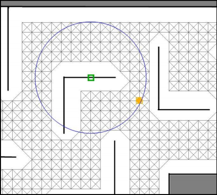
Figure 1: Conditions for the RFID tag localization procedure initialization

The presented technique for probabilistically localizing an RFID tag, is based on a two dimensional probability function $f(x,y)$, updated in each algorithmic iteration, i.e. every time the algorithm receives new information about the surrounding RFID tags.

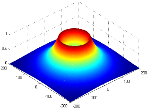
Figure 2: RFID tag pose probability distribution (axis in pixels)

During an RFID tag localization with $I\!D=i$, a circularly shaped, two dimensional probability density function $f_{t}$ is declared, having as center the current robot pose $P_{R}$ and radius equal to the distance $D$ from the RFID tag to the robot. This probability distribution has its maximum on the circumference of the circle with radius $D$, decreasing smoothly in the surrounding area. An example of the probability function is presented in figure 2.

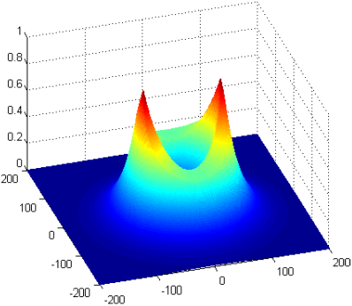
Figure 3: Product of two circular shaped probability distributions

The next step is to incorporate this distribution in the total probability distribution $f_{total}$, from which the most probable tag pose will be determined. Let’s assume that in the next data update the same tag is perceived at a distance equal to $D^{\prime}$. Of course, the robot has moved and its current pose is $P_{R}^{\prime}$. Again, a temporary probability distribution $f_{t}$, centered around $P_{R}^{\prime}$ with a radius of $D^{\prime}$ is created. Next, the total probability distribution is updated by multiplying its current values with the new information, i.e. $f_{total}=f_{total}\cdot f_{t}$. This formula constitutes another form of the Bayes probabilistic filter, described by:

$$p(x^{T}_{1:t}\,|\,z_{i:t},x^{R}_{1:t})=\alpha\cdot p(x^{T}_{t}\,|\,x^{T}_{t-1},x^{R}_{t})$$

$$\cdot p(x^{T}_{1:t-1}\,|\,z_{1:t-1},x^{R}_{1:t-1})$$ (1)

An example of two probability distributions multiplication result is visible in figure 3. Its shape – specifically the two maxima – is expected, since the initial distributions were circularly shaped and the maxima exist on the circles’ cross-sections.

This procedure is performed until the specific tag is not perceived by the robot, i.e. the distance between the robot and the tag exceeds the $3~{}m$ threshold. The localization certainty of a tag’s pose is proportional to the time perceived by the robot, measured in iterations. In figures 4(a) to 4(d) the global probability distribution for a specific RFID tag and for 30, 100, 200 and 300 iterations is depicted.

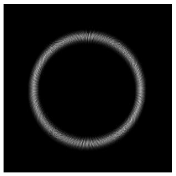
(a) Probability distribution after 30 iterations

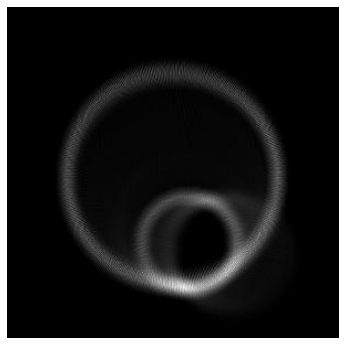
(b) Probability distribution after 100 iterations

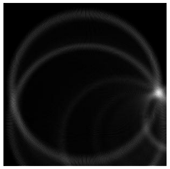
(c) Probability distribution after 200 iterations

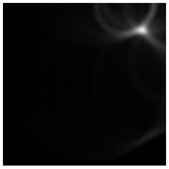
(d) Probability distribution after 300 iterations

Figure 4: Global probability distributions for a specific RFID tag for 30, 100, 200 and 300 iterations

After the final probability distribution’s calculation, the identification of the most probable tag pose is performed, as well as the specification of a way to determine whether the pose calculation is accurate. A reasonable selection would be the cell for which $f_{total}$ is maximized, which however, results in a complication in the correct pose’s probability identification. Since the distribution is not continuous (every cell holds a distinct value), the probability corresponding to a cell, is the division of its value to the sum of all the other cells, i.e.:

$$p_{x,y}=\frac{f_{total}(x,y)}{\sum_{\forall x_{i},y_{j}\in f_{total}}f_{total}(x_{i},y_{j})}$$ (2)

The problem is that due to the large number of cells participating in the distribution, $p_{x,y}$ is extremely small, even for cases where the correct pose can be obviously identified. Even though this problem is not severe, the drawback is mostly aesthetical since the calculated certainty probability does not coincide with human perception. For example, a human would identify a $90\%$ localization probability as pretty accurate, but in reality it is impossible such a value to occur. Thus, we decided to extract the probability of the cell’s surrounding area, instead out of a single pose. Specifically, if the initial probability distribution included $N\cdot M$ values, a sub sampling by $K$ is performed in order to produce $\frac{N}{3}\cdot\frac{M}{3}$ values (in our case $N=300$, $M=300$ and $K=3$). Each cell’s value is the arithmetic mean of the cells comprising the $3\times 3$ square area that surrounds it. This way, the values’ differences are “smoothed”, the number of values decreases and the actual probability calculated is quite realistic. This procedure can be mathematically supported; since the probability distribution is discrete but contains a large number of values, it can be perceived as a continuous one. As we know, in continuous distributions a point’s probability to contain a specific value is $0$. To obtain a more numerically representative value, an integration must be performed.

4 Metric Map Merging

The current work addresses the issue of merging a multi-robot team’s distributed information, whose initial poses are a priori unknown. The lack of knowledge regarding the starting positions connotes that robots lack the required reference frame to properly communicate and transform their information. Furthermore, it is assumed that robots are incapable of physically identifying each other, i.e. using cameras or distance sensors. As a result, the problem to be resolved is to specify the correct transformation – rotation and translation – between the robots’ coordinate systems, purely via common environmental information.

Our approach towards specifying the transformation is performed in three consecutive steps, to be described in detail: a) calculation of an OGM direction vector, b) calculation of the rotation quadrant and the relative translation via RFID tag information and c) exact transformation specification employing an ICP algorithm.

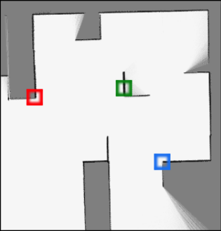
(a) First Map

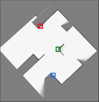
(b) Second Map

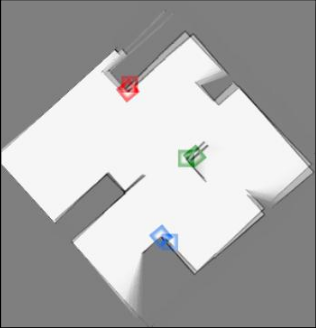
(c) Merge result

Figure 5: Example of approximate OGM merging via three common RFID tags

It should be stated that scattered RFID tags exist in the environment where the robots operate. As described in section 3, each agent can localize RFID tags using a two dimensional probability distribution. From this distribution the tag’s pose can be extracted, as well as the localization certainty. Since each RFID tag has a unique identification number, it is possible to calculate a rough transformation estimation between two coordinate systems, provided that the two robots have already localized at least three common RFID tags.

In figure 5 such a situation is presented. The first two images contain the common RFID tags in the two environments, whilst the third one presents an attempt to merge the maps, based on the RFID poses. The calculation of the exact transformation between two robots’ coordinate systems presupposes the exact RFID tags’ pose localization, something impossible, since this is performed probabilistically and not in an analytical way. Thus, the produced transformation will be approximate, since false occupancy values could exist after the map merging.

The transformation computation between two local maps is initiated when the two robots have localized at least three common RFID tags, whose localization probabilities exceed a predefined threshold. In the current work, this minimum probability value was selected equal to $75\%$. Additionally, for reasons to be analyzed further below, there is a prerequisite that one of the three RFID pairs has a quite high localization probability, whose threshold was set to $90\%$.

4.1 Relative Rotation Calculation via OGM Vectors

OGM Vector constitutes a feature originating from the environment in conjunction with an assumption. Specifically, it is assumed that the robot explores a civil environment, having a rectangular form, implying that the environmental obstacles are orthogonal to each other. An example is shown in figure 6.

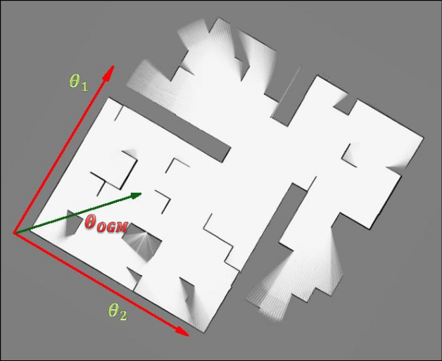
Figure 6: OGM direction vector

In this figure the two red arrows represent the two perpendicular directions $\theta_{1},\theta_{2}\,(\theta_{1}\!\!\perp\!\!\theta_{2})$, derived from the obstacles, whilst the green arrow specifies the OGM direction vector, whose orientation is equal to $\theta_{OGM}=\frac{\theta_{1}+\theta_{2}}{2}$. It should be mentioned that angles $\theta_{1},\theta_{2}$ should be bounded $\left[-\frac{\pi}{2},\frac{\pi}{2}\right]$, which results in $\theta_{OGM}\in\left[-\frac{\pi}{2},\frac{\pi}{2}\right]$. The concept behind the computation of OGM’s direction vector is the following: let’s assume that the two local OGMs are available and their relative transformation is unknown, preventing the merge. Since the robots physically exist in the same space, by determining the direction vectors $\theta_{OGM_{1}},\theta_{OGM_{2}}$ it is possible to calculate the angle $\Delta\theta_{OGM}=\theta_{OGM_{1}}-\theta_{OGM_{2}}$, which if applied to one of the maps aligns its obstacles to the other’s. It should be noted that this procedure aims at calculating a high precision approximation of the alignment angle, but not the final transformation’s rotation. This is due to the fact that the obstacles can be aligned in four different ways, one for every rotation by $\frac{\pi}{2}$. Thus, the real transformation rotation between the two maps is one of the following:

$$\Delta\theta_{OGM}=\left\{\begin{array}[]{c}\theta_{D}\\ \theta_{D}+\frac{\pi}{2}\\ \theta_{D}+\pi\\ \theta_{D}+\frac{3\pi}{2}\end{array}\right.$$

The method to specify the correct alternative out of the four possible ones, will be described in subsection 4.2.

4.1.1 RANSAC Line Detection

In order to calculate the OGM Vector, the first step is to detect the straight segments corresponding to the map’s obstacles. One of the most common methods for this purpose is the RANSAC (RAndom SAmple Consensus) algorithm. Its application is repetitive and works as such:

1. A point set $P$ is created, from which we desire to extract line segments. In our problem, $P$ contains a sub sampling of the occupied OGM cells. The sub sampling itself was performed in order to increase the method’s execution speed. In the current approach $N_{init}=|P|$.

2. Two elements of $P$ are randomly selected ($p_{1},p_{2}\in P$).

3. The line segment connecting $p_{1},p_{2}$ is calculated and all $P$’s elements having a smaller distance than a predefined threshold $D_{Line}$ from the line, are inserted in the $L$ set.

4. If $L$ contains a satisfactory percentage of $P$’s total points, i.e. if $\frac{|L|}{N_{init}}>T_{Perc}$, where $T_{perc}$ the percentage threshold, this line is registered as valid and $L$’s elements are erased from $P$. This procedure is quite flexible and can be implemented in many ways, one of which is to check $L$’s cardinality, instead of the percentage. If this condition does not apply, the algorithm returns in step 2.

5. The procedure described in steps 2-4 is executed until a predefined condition seizes to be valid. A classic condition for RANSAC termination is $\frac{|P|}{N_{init}}<T_{final}$, i.e. the points percentage not registered in any lines, divided by the initial points number, to be sufficiently small.

The RANSAC algorithm is highly parameterizable, resulting in different behaviors and execution times when different parameter sets are used. For example, if the $T_{Perc}$ value is high (e.g. more than $30\%$) and the environment is complex, the algorithm does not manage to detect any lines (or a few will be detected with difficulty). The same occurs if $T_{final}\approx 0$. Nevertheless, if $T_{Perc}$ is assigned with a very small value, a large number of lines will occur, which of course will contain an abundance of false positive cases. Aiming at minimizing the occurrence of these situations, a limitation to the algorithm iterations number is usually applied. Should the algorithm’s iterations surpass this threshold, the best so far computed line is maintained. Finally, the increment of the $D_{Line}$ threshold, implies greater tolerance of the algorithm with respect to the lines which are not entirely aligned with the two initial random points. On the contrary, if $D_{Line}$ is too small, the algorithm will not be able to detect any lines, due to failure of the $T_{Perc}$ condition.

The former analysis dictates that a careful adjustment of the algorithmic parameters is imperative, in order to achieve the goal and at the same time keep the execution times low. In our case, only a subset of the environment lines is needed, under the condition that these lines are precise. For this reason the $D_{Line}$ parameter was assigned a small value ($2~{}px$), $T_{Perc}$ a relatively high value ($15\%$) and $T_{final}$ a low value ($50\%$).

Once a line $L_{i}$ is assumed valid, its new limits are calculated. The new limits are the points which are members of the line and have the maximum distance between them:

$$\bigg{\{}p_{1}^{\prime},p_{2}^{\prime}\in L_{i}\,|\,argmax_{p_{1}^{\prime}p_{2}^{\prime}}Dist(p_{1}^{\prime},p_{2}^{\prime})\bigg{\}}$$

Thus, the real line segment’s limits are calculated, since the initial points $p_{1},p_{2}$ are probably internal. Theoretically, since the correct boundary points are calculated, the line’s gradient computed by those, is more accurate than the initial assumption. For this reason, set $P$ is recalculated containing only the elements having a maximum distance of $D_{Line}$ from the updated line. For completeness reasons, the equation to calculate a point $A$’s distance from a line, defined by two other points $B$ and $C$, follows:

$$D_{L}=\frac{|(x_{C}-x_{B})\cdot(y_{B}-y_{A})-(x_{B}-x_{A})\cdot(y_{C}-y_{B})|}{\sqrt{(x_{C}-x_{B})^{2}+(y_{C}-y_{B})^{2}}}$$ (3)

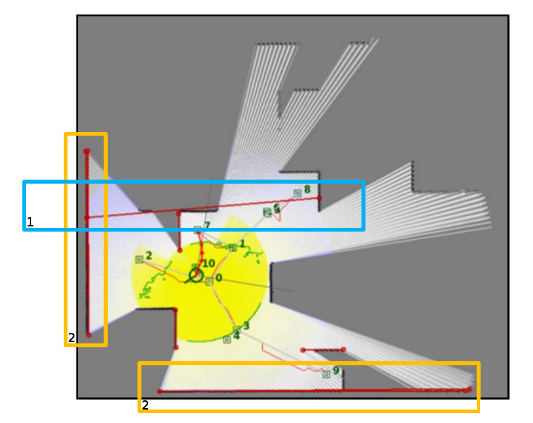
Figure 7: RANSAC-based line detection

An example of the algorithmic execution is depicted in figure 7. The first observation is that the produced lines are not representative of the overall obstacles of the environment, something expected since $T_{final}$ had a low value. Additionally, two undesirable results are detected. The first erroneous result is the line contained in the blue box (labeled with $1$), which is clearly not associated with an obstacle, but its points lie in multiple occupied surfaces. Furthermore, as evident in the orange boxes (labeled with $2$) multiple lines exist with almost equal gradient and limits. Careful observation reveals that multiple, almost identical lines exist in each box. The ideal situation would be for every line to contain points existing in a single obstacle surface. In order to overcome these drawbacks, two more algorithmic stages were implemented; the breakdown and merging of lines.

The lines breakdown refers to a segmentation procedure, regarding lines whose points lie in multiple obstacle surfaces.

Let’s assume that a check is performed in a random line $L_{i}$. For each line point $p_{j}\in L_{i}$, its distance from the first line limit $d_{j}$ is calculated and stored. Next, an ascending sort is performed in the distances. This procedure results in sorted points, the first of which are closer to the first limit and last the ones closer to the second. The next step is to traverse the distance vector and check if two successive distances’ values difference is larger than a threshold, i.e. if $|d_{k}-d_{k+1}|<D_{s}$. If this occurs, it can be safely assumed that the specific line contains elements on different obstacles. Once the latter is true, a new line is created containing the elements between the distances’ “gaps”, including the first and last point. In figure 8, the algorithmic result is depicted, assigning $D_{s}=30~{}px$.

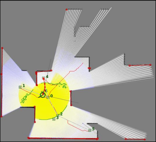
Figure 8: Line segments of the environment after the breakdown procedure

Figure 9: Line segments’ merging cases

This result indicates that the first problem risen, i.e. the existence of lines residing in multiple obstacles, is eliminated. Nevertheless, the second problem remains, as there are still obstacle surfaces represented by multiple lines with identical characteristics. For this reason, a line merging algorithm is necessary.

The algorithm that detects similar line segments and merges them is initiated by checking all lines by pairs. It is assumed that lines $L_{i},L_{j}$ are checked and their gradients are $\theta_{i},\theta_{j}$. Initially, the condition $|\theta_{i}-\theta_{j}|<T_{\theta}$ is checked, where $T_{\theta}$ is the angle threshold for two segments to be considered aligned. If this condition is met, the proximity of these lines is investigated. There are two distinct cases to be investigated, presented in figure 9.

In any of these cases, we check if the limit of the second segment nearest to the first, has a distance from it lower than a threshold $T_{j}$. If this is true, the two lines can be merged, as they are close to each other and almost parallel. The merging result is presented in figure 10.

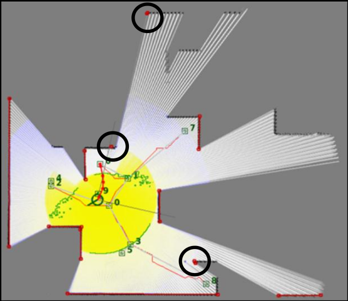
Figure 10: Line segments after the merging procedure

It is obvious that after the merging technique each obstacle is represented by a single line. An additional problem is that the resulting lines contain some erroneous ones, comprising only a few points (depicted in black circles). These result from the breakdown operations and need to be eliminated, as their gradient can be random. Additionally, a case exists (not depicted in figure 10), where a line is not entirely aligned to an obstacle surface. Since our objective is to create an accurate representation of the obstacles, i.e. line segments with accurate gradients, such misaligned behaviors must not exist, in order not to participate in the OGM direction vector’s calculation. The first part of the final test a segment must pass, is for its length to be larger than a minimum threshold, i.e. $||L_{i}||>T_{Len}$. In our implementation this was equal to $T_{Len}=30~{}px$. The second part is to check each line’s reliability. As reliability $L_{Rel}$ we define the mean arithmetic value of the occupancy probabilities of all line elements. It is obvious that the ideal case is $L_{rel}\approx 1$, where the line lies entirely on an obstacle surface. On the contrary, if $L_{rel}$ is low, this means that the line has parts not contained in any obstacle surface, thus it should be rejected. For our case $L_{rel}=0.6$.

The final result of the overall method is depicted in figure 11.

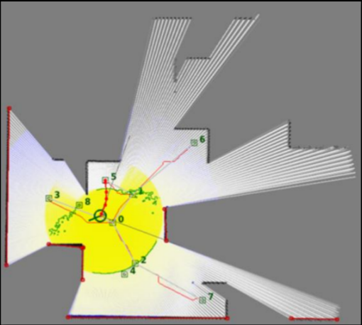
Figure 11: Line detection algorithm’s final result

4.1.2 RANSAC Line Segments Quaternion Classification

The second and final step of the OGM Vector calculation is the segments’ classification in two groups, containing perpendicular lines to each other. Whilst this is a simple concept, several problems exist regarding its implementation. A simple solution would reside to a K-Means algorithm application, which would group the angles (thus the lines) in two groups. In reality, this cannot be performed, as segments’ gradient angles are heterogeneous in value. It should be mentioned that the gradient of a segment to the horizontal axis is calculated by utilizing the inverse tangent, using the line’s extreme points. Thus, it is possible for two aligned segments to present opposite gradients (for example the first to be $89^{\circ}$ and the second $271^{\circ}$). So, even if these lines are parallel to each other, their gradient values show opposite directions. The procedure followed for the segments grouping, is based on the elimination of such cases and specifically on addition or subtraction of $\pi$ where necessary. In order to better understand the algorithm, figure 12 is presented.

The algorithm takes under assumption that the lines produced by the previous procedures are indeed perpendicular, i.e. the environment is strongly rectangular. The steps followed are:

1. The first line is taken under consideration and is denoted as $L_{G_{1}}$. At the same time, four quadrants are created based on the first line’s gradient $\theta_{1}$ (figure 12).

2. The rest of the lines are checked one at a time.

   • A segment $L_{i}$ belongs in the first group ($G_{1}$) when one of the following conditions apply:

     $$\begin{array}[]{ccc}\theta_{1}+135^{\circ}\leq&\theta_{i}&\\ \theta_{1}-45^{\circ}\leq&\theta_{i}&\leq\theta_{1}+45^{\circ}\\ &\theta_{i}&\leq\theta_{1}-135^{\circ}\end{array}$$

     If the segment’s gradient lies in the green colored quadrants, this line is stored in the first group. Additionally, in order for all the parallel segments to the first line to acquire a gradient in the first quadrant, we perform:

     $$\theta_{1}+135^{\circ}\leq\theta_{i} \Rightarrow\theta_{i}=\theta_{i}-\pi$$

     $$\theta_{i}\leq\theta_{1}-135^{\circ} \Rightarrow\theta_{i}=\theta_{i}+\pi$$

   • The same procedure is applied to the lines that belong to the second group ($G_{2}$), i.e.:

     $$\begin{array}[]{ccc}\theta_{1}+45^{\circ}\leq&\theta_{i}&\leq\theta_{1}+135^{\circ}\\ \theta_{1}-45^{\circ}\geq&\theta_{i}&\geq\theta_{1}-135^{\circ}\end{array}$$

     These lines are grouped in the quadrant where the first of them lies.

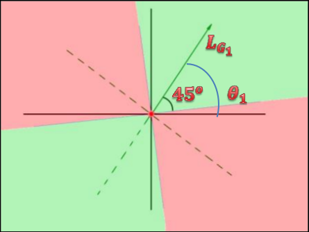
Figure 12: Creation of quadrants based on the first segment

In order to eliminate any ambiguity concerning the algorithm, an arithmetic example will be presented. Let’s assume we have identified the lines presented in table 1.

ID	$\theta_{i}$	ID	$\theta_{i}$
0	2∘	3	-89∘
1	90∘	4	179∘
2	-1∘	5	79∘

Table 1: Initial lines gradients

The steps followed are:

• The line with $ID=0$ and $\theta_{0}=2^{\circ}$ is checked. Based on this, the following quadrants are specified: $[-133^{\circ},-43^{\circ}],[-43^{\circ},47^{\circ}],[47^{\circ},137^{\circ}],[137^{\circ},-133^{\circ}]$. Obviously, the last quadrant is the merging of the two ranges $[137^{\circ},180^{\circ}]$ and $[-180^{\circ},-133^{\circ}]$, since we assume that $\theta_{i}\in\left[-180^{\circ},180^{\circ}\right]$. The line with $ID=0$ is assigned to the first group.

• The line with $ID=1$ and $\theta_{1}=90^{\circ}$ is checked. Since its gradient is in the range $[47^{\circ},137^{\circ}]$, it is assigned to the second group.

• The line with $ID=2$ and $\theta_{2}=-1^{\circ}$ is checked. Since its gradient lies in the range $[-43^{\circ},47^{\circ}]$, it is assigned to the first group.

• The line with $ID=3$ and $\theta_{3}=-89^{\circ}$ is checked. Since its gradient lies in the range $[-133^{\circ},-43^{\circ}]$, it is assigned to the second group and $\theta_{3}=\theta_{3}+\pi=91^{\circ}$.

• The line with $ID=4$ and $\theta_{4}=179^{\circ}$ is checked. Since its gradient lies in the range $[137^{\circ},-133^{\circ}]$, it is assigned to the first group and $\theta_{4}=\theta_{4}-\pi=-1^{\circ}$

• The line with $ID=5$ and $\theta_{5}=79^{\circ}$ is checked. Since its gradient lies in the range $[47^{\circ},137^{\circ}]$, it is assigned to the second group.

The lines produced after the gradient’s recalculation are visible in table 2.

ID	$\theta_{i}$	ID	$\theta_{i}$
0	2∘	3	91∘
1	90∘	4	-1∘
2	-1∘	5	79∘

Table 2: Lines gradients after classification

The next step is to calculate the direction of the two vectors defined by the obstacle line segments’ gradients. It should be reminded that, up to this point, we have accurately calculated the lines formed by the obstacles and classified them in two alignment groups.

The first group’s direction vector is calculated based on the following weighted mean:

$$\widetilde{\theta_{1}}=\frac{\sum_{\forall L_{i}\in G_{1}}\theta_{i}\cdot||L_{i}||\cdot(1-L_{Rel}^{i})}{\sum_{\forall L_{i}\in G_{1}}||L_{i}||\cdot(1-L_{Rel}^{i})}$$ (4)

This equation sums all the angles’ gradients belonging to the first group ($G_{1}$), multiplied by a coefficient. This coefficient is the line’s length, multiplied by the one’s complement of the reliability coefficient. We suppose that a long line is more reliable concerning its gradient, compared to a short one. Additionally, if a line is highly reliable, i.e. if $L_{Rel}^{i}\approx 0$, it represents quite accurately the surface it lies on. Conclusively, the direction vector of the first group is calculated via a weighted mean of this group’s lines’ gradients, weighted by coefficients indicative of the lines’ “alignment” to the obstacles. Similarly, the second group’s direction vector is calculated (denoted as $\widetilde{\theta_{2}}$). The final OGM direction vector is simply $\theta_{OGM}=\frac{\widetilde{\theta_{1}}+\widetilde{\theta_{2}}}{2}$.

4.1.3 Quadrant Determination via Common RFID Tags

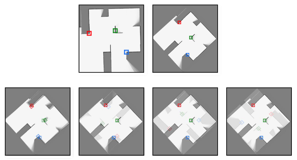
Figure 13: Top: Initial OGMs. Bottom: Four different alignment cases

Up to this point, we have determined the OGM’s direction vector. Let’s assume that two robotic agents $R_{1},R_{2}$ have reached a point where their OGMs ($M_{1},M_{2}$) must be merged. According to the described method, each OGM’s direction vector angle, $\theta_{OGM_{1}}$, $\theta_{OGM_{2}}$ is calculated. Thus, it can be inferred that if the $M_{2}$ map is rotated by an angle of $\Delta\theta_{OGM}=\theta_{OGM_{1}}-\theta_{OGM_{2}}$, the two maps’ obstacles will be aligned. Nevertheless, it is understandable, that we have achieved only the alignment and not their exact match, since this occurs for one of the following rotation angles:

$$\widehat{\Delta\theta_{OGM}}=\left\{\begin{array}[]{c}\theta_{D}\\ \theta_{D}+\frac{\pi}{2}\\ \theta_{D}+\pi\\ \theta_{D}+\frac{3\pi}{2}\end{array}\right.$$

This fact’s visualization is depicted in figure 13. As indicated, the top two images are the initial OGMs ($M_{1},M_{2}$), in which the three common RFID tags, necessary for the merging initialization, are marked. As stated, it is possible to calculate the angle $\Delta\theta_{OGM}$ by which if $M_{2}$ is rotated, its obstacles will be aligned to the ones of $M_{1}$. It is obvious that only one of the four rotation cases is valid, thus a method has to be constructed regarding its determination.

It is assumed that each robot has detected three common RFID tags, a necessary fact for the merging procedure to begin. The RFID pairs are sorted based on the pair’s minimum localization probability (an example set is depicted in table 3).

Tag ID	Localization probability of robot #1	Localization probability of robot #2	Minimum common precision	Sorting index
5	82%	92%	82%	2
7	99%	76%	76%	3
9	91%	92%	91%	1

Table 3: Example of three common RFID tags

This way, the most reliable pairs are calculated, which will be used next. Let’s assume that $t_{i}^{j}$ is the RFID tag, localized by the robot $i$ with a sorting index of $j$ and $p_{i}^{j}$ is its pose in the $M_{i}$ coordinate system. Our known variables are the three pose pairs: $\left[p_{1}^{1},p_{2}^{1}\right],\left[p_{1}^{2},p_{2}^{2}\right],\left[p_{1}^{3},p_{2}^{3}\right]$. The method followed for the correct quadrants detection, includes the determination of the lowest probability tag direction, relatively to the spatial mean of the two other high probability tag poses, in both of the coordinate systems.

Next, the quadrant occurs by subtracting the two directions. An example is visible in the figure 14.

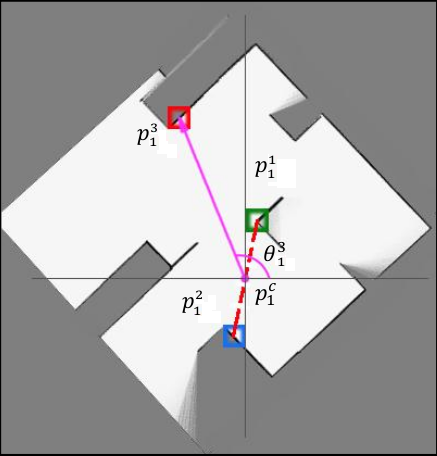
(a) First robot map and RFID tag representation

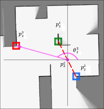
(b) Second robot map and RFID tag representation

Figure 14: OGM rotation quadrant determination

For each robot’s $R_{i}$ OGM, the following procedure is followed: Initially, the calculation of the spatial mean of the two most reliable tags (e.g. $p_{i}^{1},p_{i}^{2}$) is performed:

$$p_{i}^{c}=\left[x_{p_{i}^{c}},y_{p_{i}^{c}}\right]=\left[\frac{x_{p_{i}^{1}}+x_{p_{i}^{2}}}{2},\frac{y_{p_{i}^{1}}+y_{p_{i}^{2}}}{2}\right]$$ (5)

Next, the angle $\theta_{i}^{3}$ is calculated, which is the angle of the line segment defined by the $p_{i}^{c},p_{i}^{3}$ points.

$$\theta_{i}^{3}=\arctan(y_{p_{i}^{3}}-y_{p_{i}^{c}},x_{p_{i}^{3}}-x_{p_{i}^{c}})$$ (6)

Finally, the relative angle between the corresponding line segments in the two OGMs is $\widehat{\theta_{3}}=\theta_{1}^{3}-\theta_{2}^{3}$.

After the computation of the two direction vectors, the two desired angles $\theta_{OGM_{1}}$ and $\theta_{OGM_{2}}$ are available. The relative rotation angle by which the second robot’s map must be rotated, relatively to the first robot’s map is $\Delta\theta_{OGM}=\theta_{OGM_{1}}-\theta_{OGM_{2}}$. It is understandable that this angle is altered as such: $\widehat{\Delta\theta_{OGM}}=\theta_{OGM_{1}}-\theta_{OGM_{2}}+\kappa\frac{\pi}{2}$, where $\kappa$ is an integer in the range $[0,3]$, defining the angle correction in order not only to align the maps, but to actually merge them. The $\kappa$ coefficient is determined as follows (figure 15) :

$$\kappa=\left\{\begin{array}[]{llclc}0&\mbox{if }&\widehat{\theta_{3}}>-45^{\circ}&\mbox{ \& }&\widehat{\theta_{3}}<45^{\circ}\\ 1&\mbox{if }&\widehat{\theta_{3}}>45^{\circ}&\mbox{ \& }&\widehat{\theta_{3}}<135^{\circ}\\ 2&\mbox{if }&\widehat{\theta_{3}}>135^{\circ}&\mbox{ \& }&\widehat{\theta_{3}}<215^{\circ}\\ 3&\mbox{if }&\widehat{\theta_{3}}>215^{\circ}&\mbox{ \& }&\widehat{\theta_{3}}<305^{\circ}\\ \end{array}\right.$$ (7)

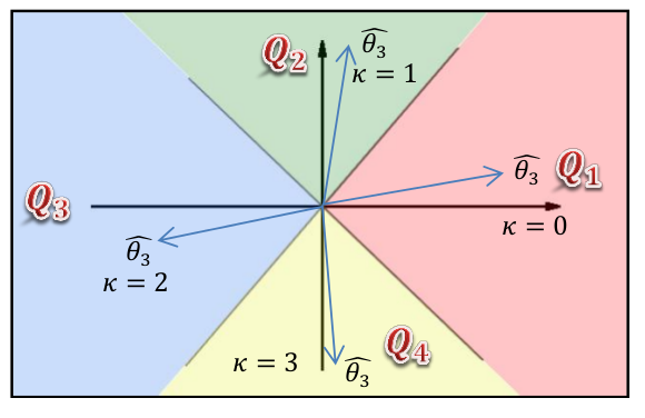
Figure 15: Determination of the correct rotation quadrant

Conclusively, up to this point, the angle $\widehat{\Delta\theta_{OGM}}=\theta_{OGM_{1}}-\theta_{OGM_{2}}+\kappa\frac{\pi}{2}$ is calculated, by which $M_{1}$ must be rotated relatively to $M_{2}$ in order for their obstacles to match. Thus the rotation of the desired transformation has been identified and the only piece of the puzzle missing is the translation.

4.2 Relative Translation Calculation via RFID Localization

The determination of the relative translation between two maps is a quite easier problem, residing in discovering a single common point in both maps. This point already exists in our case, and is the RFID tag with the highest localization probability.

Since each RFID tag is unique, we can directly associate the two maps, by aligning the two points in the corresponding coordinate systems. Additionally, as aforementioned, there is a prerequisite that the specific tag has a localization probability higher than $90\%$.

Conclusively, for the two maps to be able to merge, the following steps must occur:

• Transform $M_{2}$’s points relatively to the coordinate system created by the most reliable RFID tag (i.e. the $p_{2}^{1}$).

• Rotate these points by $\widehat{\Delta\theta_{OGM}}$ with $p_{2}^{1}$ as center.

• Translate the points relatively to the most reliable tag in $M_{1}$, whose coordinates are $\left[x_{p_{1}^{1}},y_{p_{1}^{1}}\right]$.

Thus, for a random point $[x,y]$ existing in the $M_{2}$ coordinate system, the transformation procedure into the $M_{1}$ coordinate system is:

$$\left[\begin{array}[]{c}x^{\prime}\\ y^{\prime}\end{array}\right]=R(\widehat{\Delta\theta_{OGM}})\left[\begin{array}[]{c}x-x_{p_{2}^{1}}\\ y-y_{p_{2}^{1}}\end{array}\right]+\left[\begin{array}[]{c}x_{p_{1}^{1}}\\ y_{p_{1}^{1}}\end{array}\right],$$ (8)

$R(\theta)$ denotes the two dimensional rotation matrix:

$$R(\theta)=\left[\begin{array}[]{cc}cos\theta&-sin\theta\\ sin\theta&cos\theta\end{array}\right]$$ (9)

As it will be shown next, this transformation is not quite exact. For this reason, we decided to improve the result using an ICP procedure, as described in the next section.

4.3 ICP Based Transformation Refining

The final phase of the correct transformation calculation resides in the execution of an algorithm, aiming to improve the alignment of the two maps. An ideal algorithm concerning this task is the Iterative Closest Point (ICP), utilized for the alignment of N-dimensional point sets, by the iterative approach of the two groups transformation. The scope is the minimization of the square differences between the points corresponding to the obstacles in both maps, by calculating the necessary transformation between them.

This algorithm is widely used in SLAM methods involved with scan matching, aiming at matching consecutive LRF scans, in pattern matching in the image manipulation field, or in the computer-based construction of three dimensional models. One of its largest drawbacks is its tendency to converge to local minima, something highly unlikely to occur in our case, as the two sets are already pre-aligned. Thus, ICP is utilized to correct possible alignment errors concerning the rotation angle, as the angle’s deviation is $\pm 1^{\circ}$, or in the translation derived by the high certainty RFID tag. The ICP steps follow:

1. Association creation between a point from the first group and a point of the second, which are supposed to represent common characteristics. Usually, the closest point, or the result of a k-NN (k-Nearest Neighbors) algorithm, is selected.

2. The transformation parameters are calculated, using a mean square error function.

3. The points are transformed based on the previous assumption.

4. Calculation of the total transformation till now.

5. Next algorithmic iteration.

Since we desire the best possible alignment of the two maps’ obstacles, the rational criterion of the two groups participating in the ICP algorithm, is based on the occupied pixels in each map. This way, the ICP algorithm will try to minimize the mean square error between them, achieving the best convergence. Nevertheless, this approach is not globally functional, due to the mean square error minimization process. Specifically, in order for the best converge to be achieved, the two sets must contain elements close to each other. In order to make this statement understandable, an example of two maps $M_{1}$ and $M_{2}$ is depicted in figure 16.

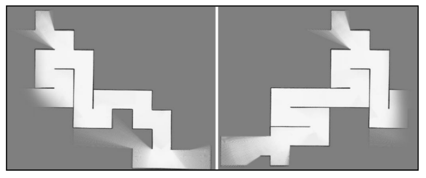
Figure 16: Example of two OGMs for merging

Additionally, let’s assume that after the transformation application (based on the OGM direction vector and the common RFID tags), we got the merging presented in figure 17.

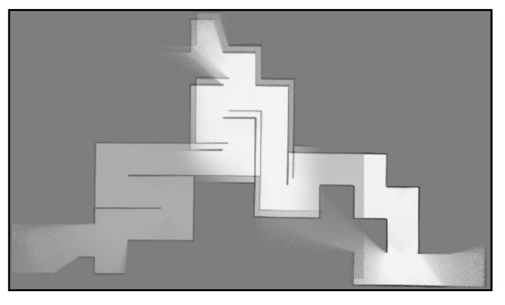
Figure 17: Approximate map merging, based on the initial transformation

The merging refinement procedure is obvious to a human being, but due to the fact that the two sets corresponding to common areas, contain very few points in comparison to the entirety of the occupied cells, it is possible for the ICP to result in total misalignment. This result is indicative of the ICP behavior to minimize the square sum error, i.e. to bring as close as possible the points of the two sets.

In order to overcome this problem, specific subsets to participate in the ICP procedure must be picked, which ought to present maximum topological similarity. Thus, the two sets’ section in terms of proximity, after the approximate transformation are selected for employment in the ICP. This way, the two final sets that will participate in the ICP algorithm, are the ones shown in the colored rectangles in figure 18.

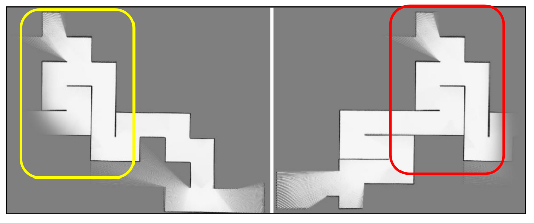
Figure 18: Common section between two OGMs

We assume that the ICP algorithm terminates with $[\Delta x_{ICP}$, $\Delta y_{ICP}$, $\Delta\theta_{ICP}]$ as a result. In conjunction to the previous transformation, the total transformation of a random point $[x,y]$ from $M_{2}$ to $M_{1}$ coordinate system is performed by the following procedure:

1. $M_{2}$’s points are relatively translated to the most reliable RFID tag, i.e. to $\left[x_{p_{2}^{1}},y_{p_{2}^{1}}\right]$.

2. These points are rotated by $\widehat{\Delta\theta_{OGM}}$.

3. The points are translated by $[\Delta x_{ICP},\Delta y_{ICP}]$.

4. The points are rotated by $\Delta\theta_{ICP}$.

5. The points are relatively translated to the $M_{1}$’s most reliable RFID tag, thus relatively to $\left[x_{p_{1}^{1}},y_{p_{1}^{1}}\right]$.

It is obvious that the ICP procedure produces a transformation intervening the one described in section 4.2. This fact occurs due to the sets ICP tries to align, which are the $M_{2}$ points, after the translation by $\left[x_{p_{2}^{1}},y_{p_{2}^{1}}\right]$ and rotation $\widehat{\Delta\theta_{OGM}}$ and the points of $M_{1}$ after their translation by $\left[x_{p_{1}^{1}},y_{p_{1}^{1}}\right]$. In mathematical notation, the exact procedure follows:

$$\left[\begin{array}[]{c}x^{\prime}\\ y^{\prime}\end{array}\right]=R(\widehat{\Delta\theta_{OGM}})\left[\begin{array}[]{c}x-x_{p_{2}^{1}}\\ y-y_{p_{2}^{1}}\end{array}\right]+\left[\begin{array}[]{c}\Delta x_{ICP}\\ \Delta y_{ICP}\end{array}\right]$$ (10)

$$\left[\begin{array}[]{c}x^{\prime\prime}\\ y^{\prime\prime}\end{array}\right]=R(\Delta\theta_{ICP})\left[\begin{array}[]{c}x^{\prime}\\ y^{\prime}\end{array}\right]+\left[\begin{array}[]{c}x_{p_{1}^{1}}\\ y_{p_{1}^{1}}\end{array}\right]$$ (11)

The combination of equations 10 and 11, after applying basic mathematics, result in:

$$\left[\begin{array}[]{c}x^{\prime\prime}\\ y^{\prime\prime}\end{array}\right]=R(\Delta\theta_{ICP}+\widehat{\Delta\theta_{OGM}})\left[\begin{array}[]{c}x\\ y\end{array}\right]+\left[\begin{array}[]{c}x_{c}\\ y_{c}\end{array}\right]$$ (12)

We observe that the final transformation formula contains the sum of two parts. Whilst the first is relative to the input, the other is constant and depends only on the two internal transformations parameters. The constant part is equal to:

$$\left[\begin{array}[]{c}x_{c}\\ y_{c}\end{array}\right]= -R(\Delta\theta_{ICP}+\widehat{\Delta\theta_{OGM}})\left[\begin{array}[]{c}x_{p_{2}^{1}}\\ y_{p_{2}^{1}}\end{array}\right]$$ (17)

$$+R(\Delta\theta_{ICP})\left[\begin{array}[]{c}\Delta x_{ICP}\\ \Delta y_{ICP}\end{array}\right]+\left[\begin{array}[]{c}x_{p_{1}^{1}}\\ y_{p_{1}^{1}}\end{array}\right]$$ (22)

4.4 Occupancy Information Merging

Even though the final transformation is accurately calculated, there is still an additional step required in order to overcome a problem introduced by the nature of the algorithm itself. Specifically, since coordinates are integer numbers (specifying cells in a grid), and should a transformation containing a rotation of arbitrary angle not equal to $0^{\circ},90^{\circ},180^{\circ}$ or $270^{\circ}$ be applied, inconsistencies due to the floating point numbers rounding will occur.

An illustration of this situation is presented in figure 19, whereas in figure 19(a) the result of two OGM and coverage fields merging is shown. Figure 19(b) indicates that after the transformation of the unoccupied cells of $M_{2}$ and their merging in $M_{1}$, the field is not smooth, but contains unexplored “gaps”. The same effect is present in the coverage map (figure 19(c)) where inconsistencies appear as well.

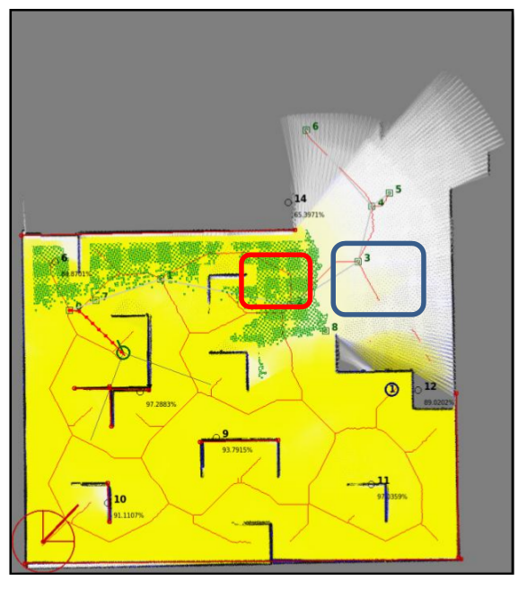
(a) Merged OGMs and Coverage fields after a geometrical transformation

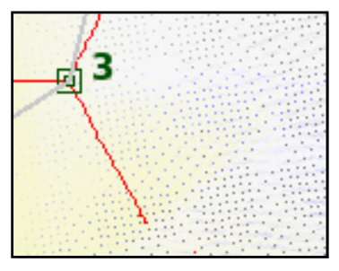
(b) Inconsistencies in the explored areas

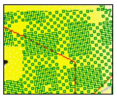
(c) Inconsistencies in the covered areas

Figure 19: Demonstration of inconsistencies due to merging

An elaborate example follows, in order to provide an adequate explanation of this phenomenon. A field of 25 two dimensional points is assumed, where $98\leq x\leq 102$ and $98\leq y\leq 102$, which is rotated by $30^{\circ}$ around the point $p_{ref}=[200,200]$ and translated in a way that $p_{ref}$ matches $p_{ref}^{\prime}=[300,300]$. This procedure is a transformation of $dx=100,dy=100,d\theta=30^{\circ}$. The points before the transformation are depicted in figure 20.

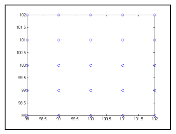
Figure 20: Coordinates field before transformation

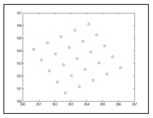
Figure 21: Points field transformation result

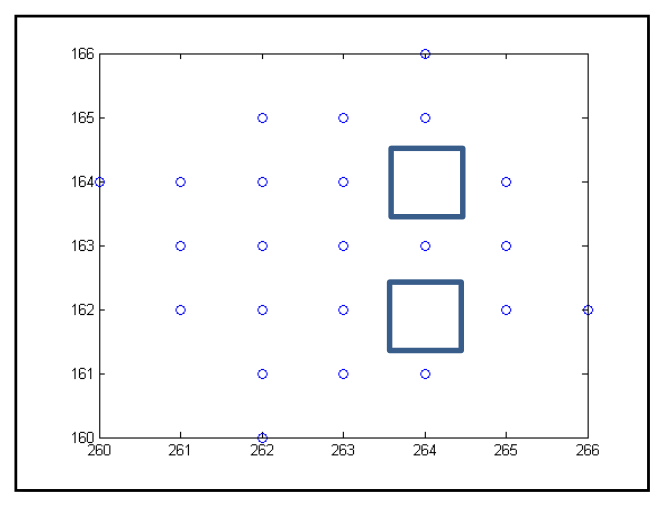
Figure 22: Points field grid transformation result

For a random point $[x,y]$, the applied transformation is:

$$\left[\begin{array}[]{c}x^{\prime}\\ y^{\prime}\end{array}\right]=R(30^{\circ})\left[\begin{array}[]{c}x-200\\ y-200\end{array}\right]+\left[\begin{array}[]{c}300\\ 300\end{array}\right]$$ (23)

This transformation’s result is depicted in figure 21. Observing this image, it is inferred that the transformation is correctly performed (symmetrically and uniformly). Nevertheless, in the specific figure, the floating point values are depicted. If this result is translated in a grid, these values must be rounded, i.e. become integer. Thus, the transformation now is:

$$\left[\begin{array}[]{c}x^{\prime}\\ y^{\prime}\end{array}\right]=\Bigg{\lfloor}R(30^{\circ})\left[\begin{array}[]{c}x-200\\ y-200\end{array}\right]+\left[\begin{array}[]{c}300\\ 300\end{array}\right]\Bigg{\rfloor}$$ (24)

The rounding result is evident in figure 22.

As expected, the final points are not uniformly distributed, as several gaps are observed in the grid (blue rectangular shapes). This fact affects both the merged OGM and the final coverage field. Concerning the merged OGM, there will be cells left unexplored in the middle of an explored area, which is undesirable. Additionally, concerning the coverage fields, the gaps affect the coverage limits.

Through observation, it is evident that the erroneous cells are presented either single or in pairs. Thus, a straightforward approach to smooth the result is to perform a blur mask (taken from the image processing field) of size $N\times N$. Since this mask will be applied on the OGM, it is necessary for $N$ to be as small as possible, or else the produced map’s detail will deteriorate. For this reason $N=3$ was selected, thus the convolution blur mask is equal to:

$$BlurMask=\frac{1}{9}\cdot\left[\begin{array}[]{ccc}1&1&1\\ 1&1&1\\ 1&1&1\end{array}\right]$$ (25)

This mask is applied to each OGM and Coverage cell, resulting in the smoothing of local pixel discontinuities. Blurring is performed after each merging among a pair of robots. A merging example, including the blurring technique is presented in figure 23(a) and a detail of it in 23(b).

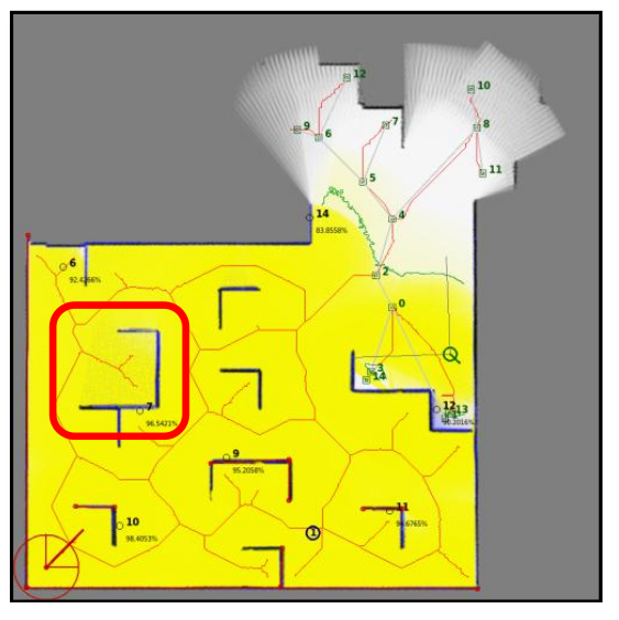
(a) Merging result, including the blurring technique

(b) Detail from the merged and blurred map

Figure 23: Blurring technique demonstration

As observed, the inconsistencies remain to a certain degree, but are quite smoothed, overcoming the problems described.

A problem occurring from the blurring approach, is the loss of the local information and specifically the large diffusion of the occupied pixels after multiple merging iterations. Next, a visualization of this new problem is presented in figure 24.

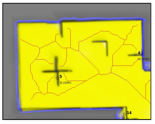
Figure 24: Diffusion effect after a large number of blurring applications

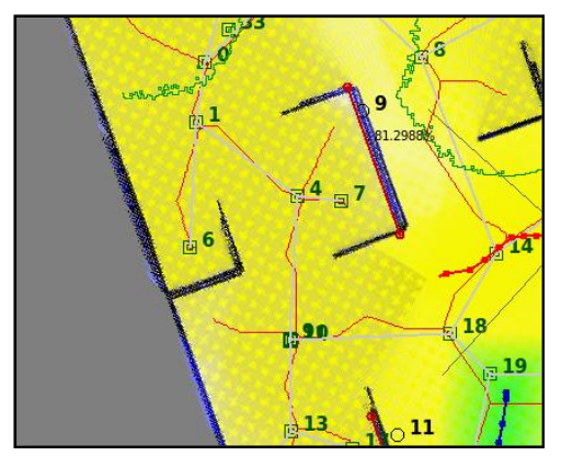
Figure 25: Final merging result

One way to surpass this problem is for the morphological blur kernel to be applied only under conditions and not in the entirety of the OGM cells. Specifically, it is necessary to apply it in the explored and unoccupied cells only, in order not to diffuse occupied values in the free space, or unoccupied values in the unexplored. After these assumptions, a sample of the final result is visible in figure 25.

5 Experiments

In this section, the experiments conducted will be presented. These are divided in two separate categories, whose combination will allow for a proper evaluation of both the overall performance and the quality of the results. Firstly, metrics and results of the OGM Vector calculation will be presented. Finally, the algorithmic performance of the algorithm in comparison with other approaches will be investigated.

The platform employed for the experiment execution was a PC with Intel Core i7 CPU at 2.80GHz, 4GB RAM, running Ubuntu 9.10 Karmic distribution.

5.1 OGM Vector Calculation

The environment used (figure 26) is an OGM, sized $700\times 600~{}px$. Every pixel occupies an area of $0.02\times 0.02~{}m^{2}$, thus the map’s dimensions in meters are $14\times 12~{}m$. The OGM direction vector algorithm was executed 1000 times and the metrics are the computed angle of the OGM vector, as well as the execution time. The results are depicted in figures 27 and 28 respectively.

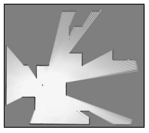
Figure 26: OGM example for direction vector calculation

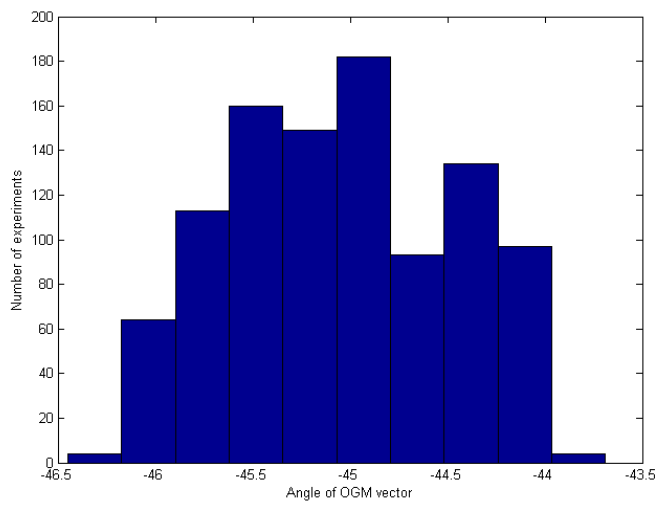
Figure 27: Diagram of the OGM vector angles

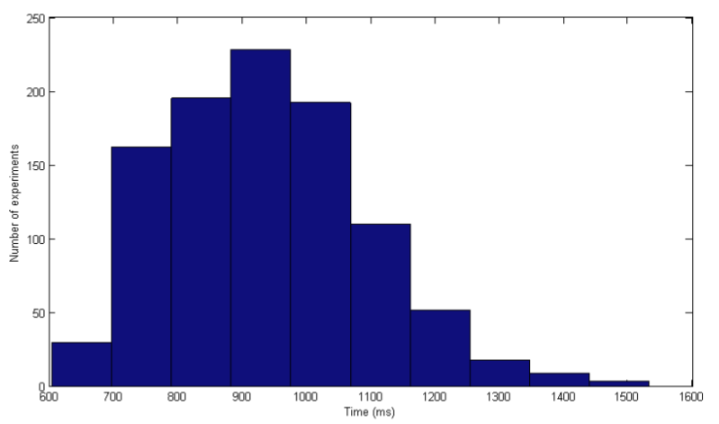
Figure 28: Diagram of the OGM vector execution times in ms

From the experimental setup, the OGM vector angle is equal to $-45^{\circ}$. The OGM direction vector’s mean angle was $-45.0497^{\circ}$ and the standard deviation was equal to $0.5598^{\circ}$. Similarly, regarding the execution times, the mean value was $938.67ms$ and the standard deviation $154.05ms$.

5.2 Map Merging

In the current section three map merging methods will be compared:

1. Transformation calculation by RFID tags

2. Transformation calculation by RFID tags and OGM direction vectors

3. Transformation calculation by RFID tags, OGM direction vectors and ICP

The first method, even though not described, is the simplest possible way to perform transformations by only using the common RFID tags. Specifically, the transformation computation resides once more in the calculation of the translation and rotation of one map relatively to another. The rotation calculation is performed similarly to the section 4.1.3, i.e. with the formula $\widehat{\theta_{3}}=\theta_{1}^{3}-\theta_{2}^{3}$, where $\theta_{i}^{3}=\arctan(y_{p_{i}^{2}}-y_{p_{i}^{c}},x_{p_{i}^{2}}-y_{p_{i}^{c}})$ and

$$p_{i}^{c}=\left[x_{p_{i}^{c}},y_{p_{i}^{c}}\right]=\left[\frac{x_{p_{i}^{1}}+x_{p_{i}^{2}}}{2},\frac{y_{p_{i}^{1}}+y_{p_{i}^{2}}}{2}\right]$$

Similarly, the translation computation is performed as such: Initially, for every tag triplet belonging to a map, their spatial mean is computed. For $M_{i}$, this is:

$$[x_{C}^{i},y_{C}^{i}]=\left[\frac{x_{p_{i}^{1}}+x_{p_{i}^{2}}+x_{p_{i}^{3}}}{3},\frac{y_{p_{i}^{1}}+y_{p_{i}^{2}}+y_{p_{i}^{3}}}{3}\right]$$ (26)

Finally, the transformation is performed by rotating $M_{2}$ by $\widehat{\theta_{3}}$ and translating it by $[x_{C}^{2}-x_{C}^{1},y_{C}^{2}-y_{C}^{1}]$.

The second method resides in the transformation computation, using the rotation computed by the OGM direction vectors for each map and the translation occurring by the most accurately localized RFID tag. Finally, the third method constitutes an extension of the second, as a further improvement step was added, the ICP algorithm. For every method, five experiments were conducted and the mean square error of the first and the transformed second map, as well as the execution time of each method were measured.

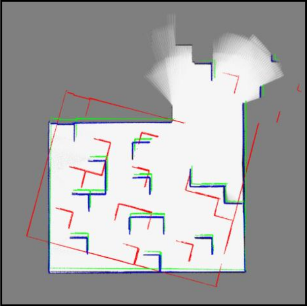
(a) Alignment example #1

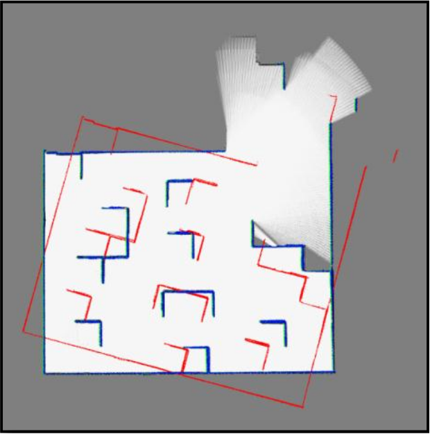
(b) Alignment example #2

Figure 29: Two alignment examples for all three methods. The first method’s result is in red color, the second method’s in green and the third method’s in blue.

Mean of five experiments	Method #1	Method #2	Method #3
Mean Square Error	7178.27 $px^{2}$	123.45 $px^{2}$	2.6 $px^{2}$
Mean Execution Time	0.026 ms	10490.8 ms	18497.6 ms

Table 4: Map merging experiments

Figure 29 indicates that the first method produces erroneous transformations that diverge a lot from the desired ones. Additionally, the second method results in satisfying transformations, since it manages to align the obstacles. Finally, the third method calculates the correct transformation, since the transformed points of the first map are exactly matched to the second.

6 Conclusions & Future Work

Initially, as far as the OGM Vector calculation is concerned, the experimental results showcase the algorithmic precision, since the angle’s mean value is extremely close to the real one. Additionally, the standard deviation is quite low, from the value of which we can assume that the $95.45\%$ of the cases have a deviation of $\pm 2\cdot\sigma=\pm 1.1196^{\circ}$, which is quite satisfactory. Regarding the execution time, its value is not low (almost a second), but by no means it is prohibitive to our application.

Regarding the map merging algorithm, the optical results inferred from figure 29 are strengthened from the mean square errors (MSE) measured, shown in table 4. It is obvious, that the first method totally fails in aligning the obstacles correctly, resulting in a large MSE, the second method has a lower error value and the third almost zero. Of course, similarly to any computational procedure, there is a counterweight regarding precision, which of course is the performance. Indeed, the experimental results indicate that the more precise the method, the larger execution time it requires. Specifically, the worst qualitative method demands the smallest execution time (a mean of 0.02 ms), since it is the simplest. The second method introduces the utilization of the RANSAC algorithm, thus the execution time increased a lot (almost 10 sec), whilst the third inserts more computations via the ICP algorithm, reaching an almost perfect aligning roughly in 18 seconds. Obviously the latter execution time is far from optimal for an on-line multi robot exploration system, but it is not prohibiting to the overall cause, since this algorithm is executed at most $N-1$ times in a $N$-agent system. Conclusively, it is preferable to spend execution resources than having a misalignment in the map merging procedure. Concerning the ICP performance issues, it would also been possible to perform the ICP algorithm, right after the transformation determination deriving only by the common RFID tags, aiming at eliminating the RANSAC procedure. This was purposefully not selected, as ICP is a very time demanding algorithm, fact supported by the experimental results, where nearly 8 seconds were spend to align almost similar points sets.

As far as future work is concerned, a similar approach can be implemented by substituting the RFID tags with other high level topological features such as corridors, doors or even with low level features such as straight line segments or corners. This way, no necessity for external devices exists, though the feature correspondence problem must be addressed. If one decides to follow the RFID approach, investigation should be performed regarding the employment of two instead of three common RFID tags, in order for the merging procedure to initiate. Even though the merging algorithm initiation conditions will be met in a shorter time period, enabling the robots to cooperate at an early exploration stage, further steps should be incorporated, as the alignment of the two local maps is now topologically ambiguous. Finally, one of the problems not addressed in this work, is the realistic RFID tag localization, as certain difficulties are introduced due to the signal cutoff or reflections. Consequently, it would be interesting to research our proposal robustness in realistic, thus more noisy, environments.

References

- [1] Stefano Carpin, Andreas Birk, ”Stochastic map merging in rescue environments”, Book : ”RoboCup 2004: Robot Soccer World Cup VIII”, p.p. 483-490, Springer-Verlag Berlin, Heidelberg ©2005
- [2] Dali Sun , Er Kleiner , Thomas M. Wendt, ”Multi-Robot Range-Only SLAM by Active Sensor Nodes for Urban Search and Rescue”, Book : ”RoboCup 2008: Robot Soccer World Cup XII”, p.p. 318 - 330, Springer-Verlag Berlin, Heidelberg ©2009
- [3] Hahnel, D., Burgard, W., Fox, D., Fishkin, K., Philipose, M., ”Mapping and localization with RFID technology”, Robotics and Automation, 2004. Proceedings. ICRA ’04. 2004 IEEE International Conference on, Vol. 1,p.p. 1015 - 1020
- [4] Kurt Konolige, Dieter Fox, Benson Limketkai, Jonathan Ko, Benjamin Stewart, ”Map Merging for Distributed Robot Navigation.”, Intelligent Robots and Systems, 2003. (IROS 2003). Proceedings. 2003 IEEE/RSJ International Conference on, p.p. 212-217 vol.1
- [5] Francesco Amigoni, Simone Gasparini and Maria Gini, ”Merging partial maps without using odometry”, Multi-Robot Systems. From Swarms to Intelligent Automata Volume III (2005), p.p. 133-144
- [6] Bonanni, Taigo Maria, Giorgio Grisseti, and Luca Iocchi. ”Merging Partially Consistent Maps” in Simulation, Modelling and Programming for Autonomous Robots, pp. 352-363. Springer International Publishing, 2014.
- [7] Saeedi, Saeed, Liam Paull, Michael Trentini, Mae Seto, and Huaqing Li. ”Group mapping: A topological approach to map merging for multiple robots.” Robotics and Automation Magazine, IEEE 21, no.2 (2014): 60-72.
- [8] Lazaro, Maria Teresa, Lina María Paz, Pedro Pinies, Jose Castellanos, and Giorgio Grisetti. ”Multi-robot SLAM using condensed measurements.” In Intelligent Robots and Systems (IROS), 2013 IEEE/RSJ International Conference on, pp. 1069-1076. IEEE, 2013.
- [9] Fox, D., Ko, J., Konolige, K., Limketkai, B., Schulz, D., Stewart, B., ”Distributed Multi-robot Exploration and Mapping”, Proceedings of the IEEE, p.p. 1325-1339, July 2006
- [10] Stefano Carpin, Andreas Birk, Viktoras Jucikas, ”On map merging”, Robotics and Autonomous Systems, Volume 53, Issue 1, 31 October 2005, p.p. 1-14
- [11] Li, Hao, Manabu Tsukada, Fawzi Nashashibi, and Michel Parent. ”Multivehicle cooperative local mapping: A methodology based on occupancy grid mapping.” Intelligent Transportation Systems, IEEE Transactions on 15, no. 5 (2014): 2089-2100.
- [12] Stefano Carpin, ”Fast and accurate map merging for multi-robot systems”, Autonomous Robots, Volume 25 Issue 3, October 2008, p.p. 305 - 316
- [13] Saeedi, Sajad, Liam Paull, Michael Trentini, Mae Seto, and Howard Li. ”Map merging using Hough peak matching.” In Intelligent Robots and Systems (IROS), 2012 IEEE/RSJ International Conference on, pp. 4683-4688. IEEE, 2012.
- [14] Keith YK Leung, Yoni Halpern, Timothy D Barfoot, Hugh HT Liu, ”The UTIAS multi-robot cooperative localization and mapping dataset”, The International Journal of Robotics Research July 2011 vol. 30 no. 8, p.p. 969-974