Analytic formulas for the rapid evaluation of the orbit response matrix and chromatic functions from lattice parameters in circular accelerators

Abstract

Measurements and analysis of orbit response matrix have been providing for decades a formidable tool in the detection of linear lattice imperfections and their correction. Basically all storage-ring-based synchrotron light sources across the world make routinely use of this technique in their daily operation, reaching in some cases a correction of linear optics down to $1\%$ beta beating and 1‰  coupling. During the design phase of a new storage ring it is also applied in simulations for the evaluation of magnetic and mechanical tolerances. However, this technique is known for its intrinsic slowness compared to other methods based on turn-by-turn beam position data, both in the measurement and in the data analysis. In this paper analytic formulas are derived and discussed that shall greatly speed up this second part. The mathematical formalism based on the Lie algebra and the resonance driving terms is extended to the off-momentum regime and explicit analytic formulas for the evaluation of chromatic functions from lattice parameters are also derived. The robustness of these formulas, which are linear in the magnet strengths, is tested with different lattice configurations.

I Introduction and motivation

Measurement and correction of focusing errors in circular accelerators is one of the top priorities in colliders and storage ring-based light sources to provide users with beam sizes and divergences as close as possible to the design values and to limit the possible detrimental effects on the beam lifetime caused by the integer and half-integer resonances. To this end, so many different techniques have been developed and successfully tested since decades that they already occupy entire chapters in textbooks Zimmermann-book . A more recent historical overview highlighting the great advancements on this domain can be found in Ro-Review .

The ever increasing BPM resolution and computing power made the analysis and correction of linear optics (focusing error and betatron coupling) via measurements of the orbit response matrix (ORM) a routine task in basically all light sources worldwide LOCO1 ; LOCO2 . Simulated ORM analysis is also carried out during the design phase of new storage-ring-based light sources for the evaluation of magnetic and mechanical tolerances SimoneThesis . Since comprehensive analytic formulas for its evaluation have not yet been found (they exist for the ideal case with no betatron coupling), the ORM response to a lattice error is computed numerically by optics codes evaluating at least one ORM for each source of error (typically quadrupole and dipole). Unless it is parallelized over several processor units, this computation becomes time-consuming in large rings and in new lattices design with even larger number of magnets. This paper aims at speeding up this computation by presenting and testing new analytic formulas for a rapid evaluation of the ORM response to linear lattice errors, with no need of orbit distortion computation.

Another known drawback of the ORM analysis is its lengthy procedure for a single measured, which typically foresees a sequence of current changes in orbit correctors and the retrieval of the corresponding orbit data. In the old (1994-2018) ESRF storage ring, this phase takes about 10 minutes for a partial ORM (32 out of 192 steerers), or 1 hour for a complete one. In larger machines such as the Large Hadron Collider (LHC) of CERN the time needed to scan the entire magnetic cycle makes this approach unsuitable for operational purposes. However, a new approach making use of alternating-current steerers, fast BPM acquisition system (at 10 kHz) and harmonic analysis of orbit data was proved to obtain the same measurement with simultaneous magnet excitations at different frequencies, hence reducing dramatically the measurement time AC-ORM ; AC-ORM2 . Still, superconducting machines like the LHC may not benefit from this ploy. These experimental aspects are not discussed in this paper.

The ORM is the main observable, though not the only ingredient for a complete analysis of linear magnetic errors. The latter do indeed modulate and generate dispersion in the horizontal and vertical planes, respectively. Analytic formulas establishing the correlations between lattice errors and linear dispersion are also inferred. The mathematical formalism developed for their derivation provides handy formulas for the computation of other chromatic functions, such as the chromatic beating (i.e. the dependence of the beta functions upon the energy deviation), chromatic coupling (i.e. how betatron coupling varies when particles go off energy) and the derivative of the dispersion function. These three quantities scale linearly with sextupole fields (normal and skew), providing a tool for the evaluation of the sextupolar model of a circular accelerators and for a fast correction of their deviations from design values.

The paper is structured as follows. The principles of the ORM analysis are presented in Sec. II for a mere sake of nomenclature. In Sec. III a new expression for the closed-orbit condition in the presence of lattice errors including betatron coupling is reported. The analytic formulas for the evaluation of the ORM and linear dispersion from linear lattice errors are presented and discussed in Sec. IV, whereas Sec. VI contains the expressions for the chromatic functions. Two schemes for the analysis of sextupolar errors based on the measurement of off-energy ORMs are eventually discussed in Sec. VII. All mathematical derivations are put in separated appendices: Appendix A for the ORM formulas and Appendix B for the chromatic functions, Appendix C for the corrections to the previous formulas accounting for the variation along magnets of the optical parameters (thick-magnet corrections).

II Quick review of the linear optics from closed orbit (LOCO)

After introducing an orbit distortion via horizontal and vertical deflections, represented by two vectors $\vec{\Theta}_{x}=(\Theta_{x,1},\ \Theta_{x,2},\ ...,\Theta_{x,N_{S}})^{T}$ and $\vec{\Theta}_{y}=(\Theta_{y,1},\ \Theta_{y,2},\ ...,\Theta_{y,N_{S}})^{T}$, where $T$ denotes the transpose and $N_{s}$ is the number of available magnets, the horizontal and vertical orbits recorded at $N_{B}$ BPMs $\vec{O}_{x}=(O_{x,1},\ O_{x,2},\ ...,O_{x,N_{B}})^{T}$ and $\vec{O}_{y}=(O_{y,1},\ O_{y,2},\ ...,O_{y,N_{B}})^{T}$ can be recorded and written as

$$\hskip 0.0pt\left(\begin{array}[]{c}\vec{O}_{x}\\ \vec{O}_{y}\end{array}\right) = \mathbf{ORM}\left(\begin{array}[]{c}\vec{\Theta}_{x}\\ \vec{\Theta}_{y}\end{array}\right),\quad\mathbf{ORM}=\left(\begin{array}[]{c c}\mathbf{O^{(xx)}}&\mathbf{O^{(xy)}}\\ \mathbf{O^{(yx)}}&\mathbf{O^{(yy)}}\end{array}\right),$$

$$O^{(xx)}_{wj}=\frac{\partial O_{x,j}}{\partial\Theta_{x,w}}\ ,\quad O^{(xy)}_{wj}=\frac{\partial O_{x,j}}{\partial\Theta_{y,w}}\ ,$$

$$O^{(yx)}_{wj}=\frac{\partial O_{y,j}}{\partial\Theta_{x,w}}\ ,\quad O^{(yy)}_{wj}=\frac{\partial O_{y,j}}{\partial\Theta_{y,w}}\ .$$

Optics codes such as MADX madx or AT AT can easily compute $\mathbf{ORM}$ for the ideal (or initial model) lattice model and the difference between the measured and expected matrix may be written as

$$\mathbf{\delta ORM} = \mathbf{ORM^{(meas)}-ORM^{(mod)}}\ .$$ (9)

The dispersion function at the BPMs (both horizontal and vertical) is also measured and its deviation from the ideal model may be computed as

$$\vec{\delta D}_{x,y}=\vec{D}_{x,y}^{(meas)}-\vec{D}_{x,y}^{(mod)}\ .$$ (10)

Both $\mathbf{\delta ORM}$ and $\vec{\delta D}_{x,y}$ depend linearly on the linear lattice errors (i.e. from bending and quadrupole magnets). By sorting the elements of each ORM block sequentially in a vector, the dependence reads

$$\left(\begin{array}[]{c}\delta\vec{O}^{(xx)}\\ \delta\vec{O}^{(yy)}\\ \delta\vec{D}_{x}\end{array}\right) = \mathbf{N}\left(\begin{array}[]{c}\delta\vec{K}_{1}\\ \delta\vec{K}_{0}\end{array}\right)\ ,$$ (16)

$$\left(\begin{array}[]{c}\delta\vec{O}^{(xy)}\\ \delta\vec{O}^{(yx)}\\ \delta\vec{D}_{y}\end{array}\right) = \mathbf{S}\left(\begin{array}[]{c}\vec{J}_{1}\\ \vec{J}_{0}\end{array}\right)\ .$$ (22)

$\delta\vec{K}_{1}$ and $\delta\vec{K}_{0}$ are the vectors containing the quadrupole and dipole errors, respectively, whereas $\vec{J}_{1}$ and $\vec{J}_{0}$ denote the skew quadrupole fields and the vertical dipole strengths. The latter may be replaced in Eq. (22) by the corresponding tilt angles $\theta$, since

$$J_{1}=-K_{1}\sin{(2\theta^{(quad)})}\ ,\quad J_{0}=-K_{0}\sin{(\theta^{(bend)})}\ .\quad$$ (23)

Throughout the paper, the MADX nomenclature for the multipolar expansion of magnetic fields is adopted,

$$-\Re\left[\sum_{n}{(K_{w,n-1}+iJ_{w,n-1})\frac{(x_{w}+iy_{w})^{n}}{n!}}\right]\ ,$$ (24)

with $K$ and $J$ referring to the integrated normal and skew magnetic strengths (normalized to the magnetic rigidity). Multipole coefficients in AT and MADX are defined differently and scaling factors depending on the multipole order need to be taken into account when converting them between the two codes. By pseudo-inverting the two systems of Eqs. (16)-(22), for instance via singular value decomposition (SVD), effective models that best fit the measured ORM and dispersion can be built. An unique model may not be extracted, since a trade-off between accuracy (i.e. large number of eigen-values in the decomposition) and reasonableness of the errors (i.e. low number of eigen-values to prevent numerical instabilities) shall be fixed on a subjective basis. Moreover, the systems of Eqs. (16)-(22) ignore contributions from the feed-down effects of quadrupoles and sextupoles induced by their misalignments and/or off-axis orbit at their locations. The closed orbit distortion resulting from this modelling renders the analysis more complex without adding values to the physical observables (betatron phase and amplitude at the the BPMs) and are usually absorbed by additional dipole errors (accounting for quadrupole misalignments) and quadrupole errors (representing the quadrupolar feed-down in sextupoles). In optics codes dipole errors induce a distortion of the reference orbit, though not of the closed one. Eqs. (16)-(22) are the core of the Linear Optics from Closed Orbit (LOCO) analysis LOCO1 ; LOCO2 . Additional fit parameters may be included in the r.h.s. of the two equations, such as calibration factors and rolls of steerers and BPMs. Once the errors ($\delta\vec{K}_{1},\ \delta\vec{K}_{0}$, $\vec{J}_{1}$ and $\vec{J}_{0}$) are included into the lattice model, the optical parameters (such as $\beta$, $\phi$, and $D$) can be computed by the optics codes and compared to the expected ones. Eqs. (16)-(22) are usually modified by inserting weights and imposing fixed tunes to obtain an effective model.

The pseudo-inversion of Eqs. (16)-(22) is a quick task. However, the overall analysis is quite time consuming, since the responses $\mathbf{M}$ and $\mathbf{S}$ of the ORM on the lattice errors ($\delta\vec{K}$ and $\vec{J}$) is usually computed by simulating an ORM for each error: A heavy computation (a few minutes) already for the old ESRF storage ring with 256 quadrupoles and 64 dipoles, which can only become more lengthy in larger machines and future light sources. If this computational time may still be tolerated when periodically correcting the linear lattice of an existing machine, it becomes the main computational overhead is simulation studies of new lattice designs, where tens of thousands of scans (including errors and corrections) are required to determine the best magnet arrangements and working point, as well as to specify (magnetic and mechanical) tolerances. Large computing farms came to the help of lattice designers in the last decade to reduce the time needed for such scan (and to increase the revenues of IT companies). The analytic formulas derived in this paper aim at further reducing the calculation time with no need of upgrading the computing farm.

III Closed orbit condition in the presence of lattice errors

Textbook formulas for the evaluation of the closed-orbit distortion induced by a dipolar perturbation are reported in Eqs. (141)- (154). Even though they still hold in the presence of focusing errors, provided that the modified Courant-Snyder (C-S) parameters are used, they do not account for betatron coupling, which transfers part of the orbit in one transverse plane in the other one. In the first part of Appendix A a condition including betatron coupling is derived. This requires an analysis in the complex domain and the introduction of some (complex) quantities. First, the complex C-S coordinates need to be introduced, $h_{z,\pm}=\tilde{z}\pm i\tilde{p}_{z}$, where $z$ stands for either $x$ or $y$ The orbit is retrieved from $h_{\pm}$ according to $z=\sqrt{\beta_{z}}\Re\{h_{z,\pm}\}$. In the decoupled complex C-S space, the linear one-turn map is represented by a diagonal matrix, $e^{i\mathbf{Q}}=\hbox{diag}(e^{2\pi iQ_{x}},e^{-2\pi iQ_{x}},e^{2\pi iQ_{y}},e^{-2\pi iQ_{y}})$. The linear transport between two elements $w$ and $j$ is represented by another phase space rotation $e^{i\mathbf{\Delta\phi}_{wj}}=\hbox{diag}(e^{i\Delta\phi_{x,wj}},e^{-i\Delta\phi_{x,wj}},e^{i\Delta\phi_{y,wj}},e^{-i\Delta\phi_{y,wj}})$, where the phase advance between $\Delta\phi_{wj}$, must be a positive quantity. However, if it is computed from the ideal betatron phases $\phi_{j}$ and $\phi_{w}$ with a fixed origin, it becomes negative whenever the position $w$ is downstream $j$: In this case the tune (i.e. the total phase advance over one turn) needs to be added, namely

$$\left\{\begin{aligned} &\Delta\phi_{x,wj}=(\phi_{x,j}-\phi_{x,w})\hskip 36.98866pt\ ,\ \hbox{if\ }\phi_{x,j}>\phi_{x,w}\\ &\Delta\phi_{x,wj}=(\phi_{x,j}-\phi_{x,w})+2\pi Q_{x}\ ,\ \hbox{if\ }\phi_{x,j}<\phi_{x,w}\end{aligned}\right.\ .\qquad$$ (25)

See Eq. (155) for more details. The effect at a generic position $j$ of focusing errors can be represented by two resonance driving terms (RDTs) prstab_esr_coupling , one for each plane:

$$\begin{aligned} f_{2000,j}=-\frac{\sum\limits_{m=1}^{M}\beta_{m,x}^{(mod)}\delta K_{m,1}e^{2i\Delta\phi_{x,mj}^{(mod)}}}{1-e^{4\pi iQ_{x}^{(mod)}}}\ +O(\delta K_{1}^{2})\\ f_{0020,j}=\frac{\sum\limits_{m=1}^{M}\beta_{m,y}^{(mod)}\delta K_{m,1}e^{2i\Delta\phi_{y,mj}^{(mod)}}}{1-e^{4\pi iQ_{y}^{(mod)}}}\ +O(\delta K_{1}^{2})\end{aligned}\quad,$$ (26)

where $\delta K_{1}$ denotes the quadrupolar errors, the sum extends over all sources of error, and the C-S parameters $\beta^{(mod)}$ and $\Delta\phi^{(mod)}$ refer to the ideal lattice, i.e. not including the above focusing errors. The remainder is proportional to $\delta K_{1}^{2}$. Betatron coupling can also be described by two RDTs,

$$\begin{aligned} f_{1001,j}=\displaystyle\frac{\sum\limits_{m=1}^{M}J_{m,1}\sqrt{\beta_{m,x}\beta_{m,y}}e^{i(\Delta\phi_{x,mj}-\Delta\phi_{y,mj})}}{4\left[1-e^{2\pi i(Q_{x}-Q_{y})}\right]}\ +O(J_{1}^{2})\\ f_{1010,j}=\displaystyle\frac{\sum\limits_{m=1}^{M}J_{m,1}\sqrt{\beta_{m,x}\beta_{m,y}}e^{i(\Delta\phi_{x,mj}+\Delta\phi_{y,mj})}}{4\left[1-e^{2\pi i(Q_{x}+Q_{y})}\right]}\ +O(J_{1}^{2})\end{aligned}\ \ ,\qquad$$ (27)

where $J_{1}$ is the skew quadrupole strength and the remainder scales with its square. The linear tunes in the above denominators shall be replaced by the eigen-tune if either resonance condition is approached. The C-S parameters $\beta$ and $\Delta\phi$ refer in this case to the lattice with focusing errors already included in the model. A complex matrix $\mathbf{B}$ containing the above four RDTs can be constructed to describe the evolution of the complex C-S coordinate vector $\vec{h}=(h_{x,-},h_{x,+},h_{y,-},h_{y,+})^{T}$:

$$\begin{aligned} &\mathbf{B}_{w}\simeq\hskip-2.84526pt\left(\begin{array}[]{c c c c}\hskip-4.2679pt1&4if_{2000,w}&\ \ 2if_{1001,w}&\ \ 2if_{1010,w}\\ \hskip-4.2679pt-4if_{2000,w}^{*}&1&-2if_{1010,w}^{*}&-2if_{1001,w}^{*}\\ \hskip-4.2679pt\ \ 2if_{1001,w}^{*}&\ \ 2if_{1010,w}&1&\ \ 4if_{0020,w}\\ \hskip-4.2679pt-2if_{1010,w}^{*}&-2if_{1001,w}&-4if_{0020,w}^{*}&1\end{array}\hskip-2.84526pt\right),\\ &\\ &\mathbf{B}_{j}^{-1}\simeq\hskip-2.84526pt\left(\begin{array}[]{c c c c}\hskip-4.2679pt1&-4if_{2000,j}&-2if_{1001,j}&-2if_{1010,j}\\ \hskip-4.2679pt\ \ 4if_{2000,j}^{*}&1&\ \ 2if_{1010,j}^{*}&\ \ 2if_{1001,j}^{*}\\ \hskip-4.2679pt-2if_{1001,j}^{*}&-2if_{1010,j}&1&-4if_{0020,j}\\ \hskip-4.2679pt\ \ 2if_{1010,j}^{*}&\ \ 2if_{1001,j}&\ \ 4if_{0020,j}^{*}&1\end{array}\hskip-2.84526pt\right),\end{aligned}$$ (28)

where the remainder in the above definitions is proportional to the square of the RDTs, whereas $w$ and $j$ refer to two generic positions along the ring. The two matrices at the same location are each other’s inverse to first order in the RDTs.

The equation for closed orbit distortion induced by $W$ horizontal and vertical deflections $\Theta_{w}$ in the complex C-S coordinates then reads

$$\vec{h}_{j} = \mathbf{B}_{j}^{-1}\sum_{w=1}^{W}\left\{\frac{e^{i\mathbf{\Delta\phi}_{wj}}}{\mathbf{1}-e^{i\mathbf{Q}}}\mathbf{B}_{w}\ \delta\vec{h}_{w}\right\}\ ,$$ (29)

where $\mathbf{1}$ is a $4\times 4$ identity matrix, and $\delta\vec{h}_{w}=(-\sqrt{\beta_{w,x}}\Theta_{w,x},\sqrt{\beta_{w,x}}\Theta_{w,x},-\sqrt{\beta_{w,y}}\Theta_{w,y},\sqrt{\beta_{w,y}}\Theta_{w,y})^{T}$. Since $O_{j}=\sqrt{\beta_{j}}\Re\{h_{j}\}$, the ORM blocks of Eq. (II) eventually read

$$\begin{aligned} &O^{(xx)}_{wj}=\sqrt{\beta_{j,x}\beta_{w,x}}\Re\left\{i\mathbf{B}_{j}^{-1}\frac{e^{i\mathbf{\Delta\phi}_{wj}}}{\mathbf{1}-e^{i\mathbf{Q}}}\mathbf{B}_{w}\right\}^{(1,1\rightarrow 2)}\ ,\\ &O^{(xy)}_{wj}=\sqrt{\beta_{j,x}\beta_{w,y}}\Re\left\{i\mathbf{B}_{j}^{-1}\frac{e^{i\mathbf{\Delta\phi}_{wj}}}{\mathbf{1}-e^{i\mathbf{Q}}}\mathbf{B}_{w}\right\}^{(1,3\rightarrow 4)}\ ,\\ &O^{(yx)}_{wj}=\sqrt{\beta_{j,y}\beta_{w,x}}\Re\left\{i\mathbf{B}_{j}^{-1}\frac{e^{i\mathbf{\Delta\phi}_{wj}}}{\mathbf{1}-e^{i\mathbf{Q}}}\mathbf{B}_{w}\right\}^{(3,1\rightarrow 2)}\ ,\\ &O^{(yy)}_{wj}=\sqrt{\beta_{j,y}\beta_{w,y}}\Re\left\{i\mathbf{B}_{j}^{-1}\frac{e^{i\mathbf{\Delta\phi}_{wj}}}{\mathbf{1}-e^{i\mathbf{Q}}}\mathbf{B}_{w}\right\}^{(3,3\rightarrow 4)}\ .\end{aligned}\qquad$$ (30)

In the above notation, given a $4\times 4$ matrix $\mathbf{A}$, $\mathbf{A}^{(a,b\rightarrow c)}=A_{ac}-A_{ab}$.

If focusing errors are included in the model, $f_{2000}=f_{0020}=0$ anywhere along the ring and the more explicit expressions for the four ORM blocks of Eq. (214) can be derived.

IV Analytic formulas for the evaluation of ORM and linear dispersion from lattice parameters

Equation (30) is further expanded in Appendix A to derive the ORM response to a focusing error and to a skew quadrupole field, i.e. to infer the betatronic blocks of the matrices $\mathbf{N}$ and $\mathbf{S}$ of Eqs. (16)-(22). As far as the former is concerned, the expressions truncated to first order in $\delta K_{1}$ for the two diagonal blocks read

$$N^{(xx)}_{wj,m} \simeq -\frac{\sqrt{\beta_{j,x}^{(mod)}\beta_{w,x}^{(mod)}}\beta_{m,x}^{(mod)}}{2\sin{(\pi Q_{x}^{(mod)})}}\Bigg{\{}\frac{\cos{(\tau_{x,wj}^{(mod)})}}{4\sin{(2\pi Q_{x}^{(mod)})}}\Big{[}\cos{(2\tau_{x,mj}^{(mod)})}+\cos{(2\tau_{x,mw}^{(mod)})}\Big{]}$$ (31)

$$\hskip 102.43008pt+\frac{\ \sin{(\tau_{x,wj}^{(mod)})}}{4\sin{(2\pi Q_{x}^{(mod)})}}\Big{[}\sin{(2\tau_{x,mj}^{(mod)})}-\ \sin{(2\tau_{x,mw}^{(mod)})}\Big{]}$$

$$\hskip 102.43008pt+\frac{1}{2}\sin{(\tau_{x,wj}^{(mod)})}\left[\Pi(m,j)-\Pi(m,w)+\Pi(j,w)\right]+\frac{\cos{(\Delta\phi_{x,wj}^{(mod)})}}{4\sin{(\pi Q_{x}^{(mod)})}}\Bigg{\}}\ ,$$

$$N^{(yy)}_{wj,m} \simeq +\frac{\sqrt{\beta_{j,y}^{(mod)}\beta_{w,y}^{(mod)}}\beta_{m,y}^{(mod)}}{2\sin{(\pi Q_{y}^{(mod)})}}\Bigg{\{}\frac{\cos{(\tau_{y,wj}^{(mod)})}}{4\sin{(2\pi Q_{y}^{(mod)})}}\Big{[}\cos{(2\tau_{y,mj}^{(mod)})}+\cos{(2\tau_{y,mw}^{(mod)})}\Big{]}$$

$$\hskip 102.43008pt+\frac{\ \sin{(\tau_{y,wj}^{(mod)})}}{4\sin{(2\pi Q_{y}^{(mod)})}}\Big{[}\sin{(2\tau_{y,mj}^{(mod)})}-\ \sin{(2\tau_{y,mw}^{(mod)})}\Big{]}$$

$$\hskip 102.43008pt+\frac{1}{2}\sin{(\tau_{y,wj}^{(mod)})}\left[\Pi(m,j)-\Pi(m,w)+\Pi(j,w)\right]+\frac{\cos{(\Delta\phi_{y,wj}^{(mod)})}}{4\sin{(\pi Q_{y}^{(mod)})}}\Bigg{\}}\ ,$$

where the function $\Pi$ is defined as

$$\Pi(a,b)=1\quad\hbox{if\ }s_{a}<s_{b}\ ,\quad\Pi(a,b)=0\quad\hbox{if\ }s_{a}\geq s_{b}\ .\qquad$$ (32)

The quantity $\tau_{ab}$ is a mere shifted phase advance between two locations $a$ and $b$,

$$\tau_{z,ab}=\Delta\phi_{z,ab}-\pi Q_{z}\ ,\quad z=x,y\quad,$$ (33)

where the phase advance $\Delta\phi_{wj}$ is evaluated as usual according to Eq. (25).

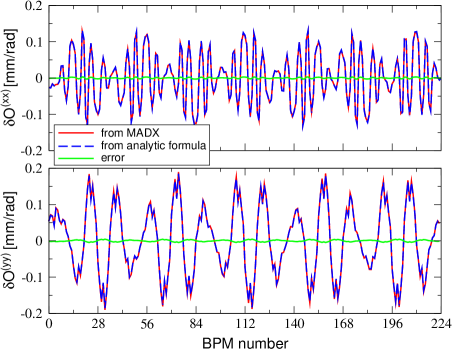
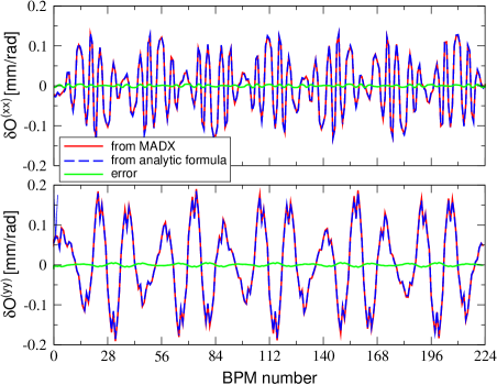
Figure 1: (Color) $\delta\vec{O}^{(xx)}$ and $\delta\vec{O}^{(yy)}$ induced by a steerer (horizontal and vertical, respectively) in the presence of a single quadrupole error inducing an rms beta beating of $6.9\%$ and $2.2\%$ in the two planes (top 2 plots) and with an additional source of betatron coupling generating an emittance ratio $\mathscr{E}_{y}/\mathscr{E}_{x}\simeq 1\%$ (bottom 2 plots). The red curves result from the computation of the orbit distortion by MADX, whereas the blue dashed lines are derived from Eqs. (31) and (35) which do not require any orbit calculation. The agreement between the two evaluations is within $3\%$ rms. The lattice of the old ESRF storage ring has been used.

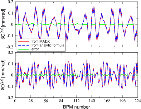
Figure 2: (Color) $\delta\vec{O}^{(xy)}$ and $\delta\vec{O}^{(yx)}$ induced by a steerer (vertical and horizontal, respectively) in the presence of an rms beta beating of $6.9\%$ and $2.2\%$ in the two planes and a single skew quadrupole error generating an emittance ratio $\mathscr{E}_{y}/\mathscr{E}_{x}\simeq 1\%$. The red curves result from the computation of the orbit distortion by MADX, whereas the blue dashed lines are derived from Eqs. (38)- (39) which do not require any orbit calculation. The agreement between the two evaluations is within $2\%$ rms if the C-S parameters including focusing errors are used in Eq. (39) (top 2 plots), whereas it increases up to $7\%$ rms if the ideal lattice parameters (of the old ESRF storage ring in this case) are used (bottom 2 plots).

Equation (31) describes the response of a $\mathbf{\delta}$ORM diagonal block element $wj$ (where $w$ refers to the steerer and $j$ to the BPM) to a quadrupole error $m$, namely

$$N^{(xx)}_{wj,m}=\frac{\delta O^{(xx)}_{wj}}{\delta K_{m,1}}\quad,\quad N^{(yy)}_{wj,m}=\frac{\delta O^{(yy)}_{wj}}{\delta K_{m,1}}\quad.$$ (34)

The deviation of the ORM diagonal blocks from the ideal values are then computed according to

$$\delta O^{(xx)}_{wj}\simeq\sum_{m=1}^{M}N^{(xx)}_{wj,m}\delta K_{m,1}\ ,\ \delta O^{(yy)}_{wj}\simeq\sum_{m=1}^{M}N^{(yy)}_{wj,m}\delta K_{m,1}\ .$$

(35)

Note that all C-S parameters $\beta^{(mod)}$ and $\Delta\phi_{wj}^{(mod)}$ refer to the ideal or initial lattice model, implying that the responses $N^{(xx)}_{wj,m}$ and $N^{(yy)}_{wj,m}$ can be computed post-processing a single output file or table from any optics code, with no need of launching it to compute the ORM for each quadrupolar error. The phase advance $\Delta\phi_{wj}$ is evaluated according to Eq. (25).

In Fig. 1 two examples are reported showing the deviation of one column of the ORM diagonal blocks from the ideal model, $\delta\vec{O}^{(xx)}$ and $\delta\vec{O}^{(yy)}$, at the 224 BPMs of the old ESRF storage ring. The two blocks are computed from the direct evaluation by MADX of the orbit distortion induced by two steerers in the presence of an error in one thick quadrupole, $\delta K_{1}=5\times 10^{-3}$ m^-1 (red curves), as well as from Eqs. (31) and (35) (blue dashed curves). In the former case, two complete ORMs need to be computed (with and without the quadrupole error), whereas the two formulas require a single evaluation of the ideal C-S parameters and a few lines of post-processing code: a computation by far much faster than the direct calculation of the ORM. The rms error of the ORM blocks computed via Eqs. (31) and (35) with respect to the direct computation of the matrices is within $3\%$. The quadrupole error induces an rms beta beating of $6.9\%$ and $2.2\%$ in the two planes (top 2 plots). The addition of a skew quadrupole inducing a ratio between the two transverse equilibrium emittances $\mathscr{E}_{y}/\mathscr{E}_{x}\simeq 1\%$ (bottom 2 plots of Fig. 1) does not deteriorate the level of accuracy.

The expressions in Eq. (31) have been derived assuming a constant value of the beta function ($\beta_{m}$) across a generic quadrupole $m$, usually computed at its center. The phase advance $\Delta\phi_{mj}$ between the magnet and a generic location $j$ refers to its center too. This approximation may not be sufficiently accurate in general and in particular for lattices comprising combined-function magnets, along which the beta function varies considerably. In Appendix C corrections accounting for that variation are derived assuming hard-edged quadrupoles (i.e. ignoring fringe fields). The terms to be replaced in Eq. (31) are

$$\begin{aligned} \beta_{m}\hskip 1.42262pt&\longrightarrow\hskip 1.42262ptI_{\beta,m}\\ \beta_{m}\sin{(2\tau_{mj})}\hskip 1.42262pt&\longrightarrow\hskip 1.42262ptI_{S,mj}\ \ ,\quad\beta_{m}\cos{(2\tau_{mj})}\hskip 1.42262pt\longrightarrow\hskip 1.42262ptI_{C,mj}\ \ ,\\ \beta_{m}\sin{(2\tau_{mw})}\hskip 1.42262pt&\longrightarrow\hskip 1.42262ptI_{S,mw}\ ,\quad\beta_{m}\cos{(2\tau_{mw})}\hskip 1.42262pt\longrightarrow\hskip 1.42262ptI_{C,mw}\ ,\end{aligned}$$

where $I_{\beta,m}$, $I_{C,m}$ and $I_{S,m}$ are computed from the quadrupole coefficients (length and non-integrated strength) and C-S parameters at the magnet entrance ($s_{m}$) according to Eqs. (547)-(550). An even more general case is considered where the quadrupolar field error is sought in other type of magnets (such as steerers and nonlinear elements): The corresponding expressions for the above integrals are given in Eqs. (556)-(559). As far as the old ESRF storage ring is concerned, which does not include combined-function magnets, the above corrections reduce the rms error of Eqs. (31) and (35) by about a factor 2. Steerers $w$ are also assumed to be of zero length in Eq. (31). A further generalization accounting for thick deflectors is also presented in Sec. C.7 at the end of Appendix C.

The response of a $\mathbf{\delta}$ORM off-diagonal block element $wj$ to a skew quadrupole $m$ can be written as

$$S^{(xy)}_{wj,m}=\frac{\partial O^{(xy)}_{wj}}{\partial J_{m,1}}\quad,\quad S^{(yx)}_{wj,m}=\frac{\partial O^{(yx)}_{wj}}{\partial J_{m,1}}\quad.$$ (37)

Assuming an uncoupled ideal (or initial) lattice model, the deviation of the ORM off-diagonal blocks from the ideal values (which are zeros) corresponds to the block themselves and can be evaluated according to

$$\delta O^{(xy)}_{wj}\simeq\sum_{m=1}^{M}S^{(xy)}_{wj,m}J_{m,1}\ ,\ \delta O^{(yx)}_{wj}\simeq\sum_{m=1}^{M}S^{(yx)}_{wj,m}J_{m,1}\ ,$$

(38)

where the remainders scales with $J_{1}^{2}$ and the matrix elements $S^{(xy)}_{wj,m}$ and $S^{(yx)}_{wj,m}$ read

$$S^{(xy)}_{wj,m} \simeq \frac{1}{8}\sqrt{\beta_{j,x}\beta_{w,y}\beta_{m,x}\beta_{m,y}}\left\{\frac{1}{\sin{[\pi(Q_{x}-Q_{y})]}}\left[\frac{\cos{(\tau_{x,mj}-\tau_{y,mj}+\tau_{y,wj})}}{\sin{\pi Q_{y}}}-\frac{\cos{(\tau_{x,mw}-\tau_{y,mw}+\tau_{x,wj})}}{\sin{\pi Q_{x}}}\right]\right.$$ (39)

$$\hskip 92.47145pt\left.+\frac{1}{\sin{[\pi(Q_{x}+Q_{y})]}}\left[\frac{\cos{(\tau_{x,mj}+\tau_{y,mj}-\tau_{y,wj})}}{\sin{\pi Q_{y}}}+\frac{\cos{(\tau_{x,mw}+\tau_{y,mw}+\tau_{x,wj})}}{\sin{\pi Q_{x}}}\right]\right\}\ ,$$

$$S^{(yx)}_{wj,m} \simeq \frac{1}{8}\sqrt{\beta_{j,y}\beta_{w,x}\beta_{m,x}\beta_{m,y}}\left\{\frac{1}{\sin{[\pi(Q_{x}-Q_{y})]}}\left[-\frac{\cos{(\tau_{x,mj}-\tau_{y,mj}-\tau_{x,wj})}}{\sin{\pi Q_{x}}}+\frac{\cos{(\tau_{x,mw}-\tau_{y,mw}-\tau_{y,wj})}}{\sin{\pi Q_{y}}}\right]\right.$$

$$\hskip 92.47145pt\left.+\frac{1}{\sin{[\pi(Q_{x}+Q_{y})]}}\left[\frac{\cos{(\tau_{x,mj}+\tau_{y,mj}-\tau_{x,wj})}}{\sin{\pi Q_{x}}}+\frac{\cos{(\tau_{x,mw}+\tau_{y,mw}+\tau_{y,wj})}}{\sin{\pi Q_{y}}}\right]\right\}\ .$$

Note that all C-S parameters $\beta$ and $\Delta\phi_{wj}$ refer this time to the lattice model including the focusing errors, quadrupolar error. This requires that the analysis of Eq. (16) is carried out before matching the measured ORM off-diagonal blocks of Eq. (22). If the ideal (or initial) C-S parameters are used, the accuracy of Eq. (39) is deteriorated.

As expected, when either tune approaches the integer or half-integer resonance, both Eqs. (31)-(39) diverge. In the presence of betatron coupling the same is true for the off-diagonal ORM blocks $\delta\vec{O}^{(xy)}$ and $\delta\vec{O}^{(yx)}$ of Eq. (39), when the sum resonance is approached, i.e. $Q_{x}+Q_{y}\simeq N$, where N in an integer. On the other hand, the denominators dependent on $(Q_{x}-Q_{y})$ do not diverge when the difference resonance is approached, since the eigen-tunes remain separated by $\Delta Q_{min}$.

In Fig. 2 an example of deviation of one column from the ORM diagonal off-blocks $\delta\vec{O}^{(xy)}$ and $\delta\vec{O}^{(yx)}$ evaluated by MADX and Eqs. (38)-(39) is displayed, along with the errors of the analytic formulas. When the C-S parameters including focusing errors are used in Eq. (39) the relative rms error is of about $2\%$ (top 2 plots), whereas it increases to $7\%$ if the ideal C-S parameters are used. This confirms the need of evaluating the focusing error model (from the ORM diagonal blocks) before fitting the off-diagonal blocks.

If the variation of $\beta$ and $\tau$ along the skew (or tilted) quadrupole $m$ is to be taken into account, the same procedure described in Appendix C can be followed. The cosine terms of Eq. (39) can be manipulated so to factorize the ones dependent on the magnet $m$ only, and replace them with their integrals, namely

$$\begin{aligned} \sqrt{\beta_{m}}\sin{\tau_{mj}}&\longrightarrow&J_{S,mj}\ ,\\ \sqrt{\beta_{m}}\cos{\tau_{mj}}&\longrightarrow&J_{C,mj}\ .\end{aligned}$$ (40)

These integrals can be computed analytically via Eq. (569)-(570) and inserted in Eq. (39). If the variation of the C-S parameters across the steerer $w$ is to be taken into account, the same procedure carried out in Sec. C.7 at the end of Appendix C can be followed (not reported here).

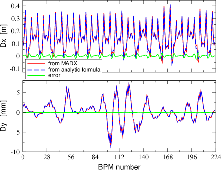
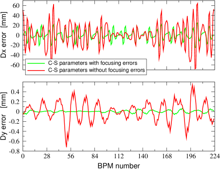
Figure 3: (Color) Top 2 plots: Dispersion function computed by MADX (PTC module) and by Eq. (41) for the lattice of the old ESRF storage ring comprising a model of focusing errors and betatron coupling inferred from an ORM measurement. The bottom two plots show the error of Eq. (41) with different lattice parameters: from the model including the focusing errors (black), from the ideal model (red), and from the model with edge focusing from dipoles on top of the previous set of focusing errors (green). In the first and latter cases the relative error is within $10\%$ and $1.5\%$ for $D_{x}$ and $D_{y}$, respectively.

In Appendix B an analytic expression to evaluate the linear dispersion at a generic location $j$ in the presence of betatron coupling is derived:

$$\begin{aligned} D_{x}(j)&\simeq+\frac{\sqrt{\beta_{j,x}}}{2\sin{(\pi Q_{x})}}\sum_{m=1}^{M}\left(K_{m,0}+J_{m,1}D_{m,y}\right)\sqrt{\beta_{m,x}}\times\\ &\hskip 91.04872pt\cos(\tau_{x,mj})\ ,\\ D_{y}(j)&\simeq-\frac{\sqrt{\beta_{j,y}}}{2\sin{(\pi Q_{y})}}\sum_{m=1}^{M}\left(J_{m,0}-J_{m,1}D_{m,x}\right)\sqrt{\beta_{m,y}}\times\\ &\hskip 91.04872pt\cos(\tau_{y,mj})\ ,\end{aligned}$$ (41)

where $\tau$ is the same shifted phase advance of Eq. (33) and the dispersion function at the magnets $D_{m}$ refers to the uncoupled lattice, i.e. that generated by horizontal and vertical bending magnets ($K_{0}$ and $J_{0}$ for $D_{m,x}$ and $D_{m,y}$, respectively). $D_{m}$ shall then be computed from the above equations putting $J_{m,1}=0$ and then inserted in the complete formulas to obtain the final dispersion $D(j)$. Equation (41) indeed describes the entanglement between the horizontal and vertical dispersion functions due to skew quadrupole fields. In the presence of focusing errors the above equations are still valid, provided that the corresponding C-S parameters $\beta$, $\phi$ and dispersion are used. If the ideal lattice parameters are inserted, a larger error is to be expected. In Fig. 3 an example is shown with the dispersion function computed by MADX (PTC module) and by Eq. (41) for the lattice of the old ESRF storage ring comprising a model of focusing errors and betatron coupling inferred from an ORM measurement. If the C-S parameters including focusing errors are used, the rms error is within $10\%$ and $1\%$ for $D_{x}$ and $D_{y}$, respectively, whereas it increases to $25\%$ and $10\%$ if the ideal C-S parameters are used in Eq. (41).

In Eq. (41) constant C-S parameters and dispersion across the magnet $m$ are assumed. In order to account for their variation, the latter can be divided in several sub-elements to better retrieve the correct profile of those functions (Fig. 3 is obtained after slicing the magnets in twenty elements). Once again, analytic expressions exist to overcome this inconvenience and are derived in Appendix C. The terms to be replaced in Eq. (41) are

$$\begin{aligned} \sqrt{\beta_{m}}\cos{(\tau_{mj})}&\hskip 1.42262pt\longrightarrow\hskip 1.42262ptJ_{C,mj}\ ,\\ \sqrt{\beta_{m,x}}D_{m,y}\cos{(\tau_{x,mj})}&\hskip 1.42262pt\longrightarrow\hskip 1.42262ptJ_{C,mj}^{(D_{y})}\ ,\\ \sqrt{\beta_{m,y}}D_{m,x}\cos{(\tau_{y,mj})}&\hskip 1.42262pt\longrightarrow\hskip 1.42262ptJ_{C,mj}^{(D_{x})}\ ,\end{aligned}\qquad$$ (42)

where $J_{C,mj}$ is computed via Eqs. (566)-(567) for pure (sector) bending magnets and via Eqs. (569)-(570) for combined-functions magnets. $J_{C,mj}^{(D_{y})}$ and $J_{C,mj}^{(D_{x})}$ depend instead on the (skew or tilted) quadrupole parameters and can be evaluated from Eq. (587). As shown by Eqs. (566)-(567) of Appendix C, $J_{C,mj}$ exhibits a dependence on the bending angle $K_{m,0}$, which can be ignored as long as $K_{m,0}\ll 1$, i.e. for large rings. On the other hand, in small rings with strong bending angles, the dependence of the dispersion function on $K_{m,0}$ becomes nonlinear. The effectiveness of the thick-magnet correction of Eq. (42) can be appreciated in Fig. 4: In this example, the rms error turns out to be one order of magnitude lower than the one obtained by using Eq. (41) after slicing all magnets in twenty parts.

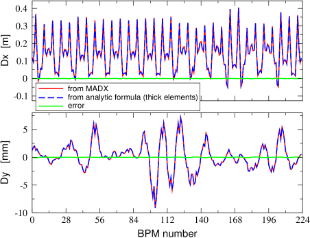
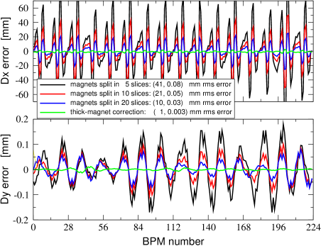
Figure 4: (Color) Top 2 plots: The same dispersion function of Fig. 3 computed by MADX (PTC module) and by Eq. (41) with the thick-magnet correction of Eq. (42). The bottom two plots show the dependence of the error on the number of magnet slices for Eq. (41) compared to (much lower) discrepancy of Eq. (42). In the legend, rms errors are given for $D_{x}$ and $D_{y}$, respectively.

From Eq. (41) the $D_{x}$ response to a dipole error $\delta K_{0}$, and the one of $D_{y}$ on vertical dipole fields $J_{0}$ and skew quadrupole strength $J_{1}$ can be easily inferred.

$$\begin{aligned} N_{j,m}^{(\delta K_{0}\rightarrow D_{x})}&\simeq+\frac{\sqrt{\beta_{j,x}}}{2\sin{(\pi Q_{x})}}\left\{\sqrt{\beta_{m,x}}\cos(\tau_{x,mj})\right\}\ ,\\ S_{j,m}^{(J_{0}\rightarrow D_{y})}&\simeq-\frac{\sqrt{\beta_{j,y}}}{2\sin{(\pi Q_{y})}}\left\{\sqrt{\beta_{m,y}}\cos(\tau_{y,mj})\right\}\ ,\\ S_{j,m}^{(J_{1}\rightarrow D_{y})}&\simeq+\frac{\sqrt{\beta_{j,y}}}{2\sin{(\pi Q_{y})}}\left\{\sqrt{\beta_{m,y}}D_{m,x}\cos(\tau_{y,mj})\right\}\ .\end{aligned}$$ (43)

If needed, the terms in the above curly brackets can be replaced by the thick-magnet corrections of Eq. (42). The dispersive parts of Eqs. (16)-(22) then read

$$\begin{aligned} \delta D_{j,x}&=\sum_{m=1}^{M}N_{j,m}^{(\delta K_{0}\rightarrow D_{x})}\delta K_{m,0}\ ,\\ \delta D_{j,y}&=\sum_{m=1}^{M}\left(S_{j,m}^{(J_{0}\rightarrow D_{y})}J_{m,0}+S_{j,m}^{(J_{1}\rightarrow D_{y})}J_{m,1}\right)\ .\end{aligned}$$ (44)

The contribution to $\delta D_{x}$ stemming from the product $J_{m,1}D_{m,y}$ in Eq. (41) has been ignored as it is of a perturbation of second order.

In conclusion, Eqs. (31), (39) and (43) provide explicit expressions to evaluate the ORM and dispersion response matrices $\mathbf{N}$ and $\mathbf{S}$ of Eqs. (16)-(22) from lattice parameters with no need of evaluating any ORM.

The impact of sextupoles in the measurement of the ORM is discussed in Sec. A.3 of Appendix A. The orbit distortion induced by steerer magnets generates normal and skew quadrupole feed-down fields, $\delta K_{1}=-K_{2}x_{\rm c.o.}$ and $J_{1}=K_{2}y_{\rm c.o.}$, where $K_{2}$ denotes the integrated strength of a generic sextupole and $(x_{\rm c.o.},\ y_{\rm c.o.})$ is the corresponding closed orbit. Dipolar feed-down fields proportional to $(x_{\rm c.o.}^{2},\ y_{\rm c.o.}^{2})$ are also generated. It is demonstrated that if the ORM is measured via a double symmetric distortion $\pm\theta_{w}$, the quadrupolar feed-down generated by sextupoles is canceled out, leaving a residual error proportional to $\theta_{w}^{2}$ (a few permil rms for the old ESRF storage ring).

V Analytic formulas for the phase advance shifts induced by quadrupole errors

An alternative to the ORM for the linear analysis of lattice errors is the measurement and fit of the BPM phase advances obtained from turn-by-turn data. In Ref. Andrea-Linear-arxiv analytic formulas relating the actual betatron phase advance to the ideal one (from the model), detuning terms and the RDTs were derived. In Appendix B those formulas have been further manipulated so to make the dependence of the phase advance on the quadrupole errors $\delta K_{1}$ explicit, yielding

$$\begin{aligned} \Delta\phi_{x,wj}&\simeq\Delta\phi_{x,wj}^{(mod)}+\sum_{m=1}^{M}\delta K_{m,1}\frac{\beta_{m,x}^{(mod)}}{4}\\ &\hskip 14.22636pt\times\Bigg{\{}2\Big{[}\Pi(m,j)-\Pi(m,w)+\Pi(j,w)\Big{]}\\ &\hskip 28.45274pt+\frac{\sin{(2\tau_{x,mj}^{(mod)})}-\sin{(2\tau_{x,mw}^{(mod)})}}{\sin{(2\pi Q_{x}^{(mod)})}}\Bigg{\}}\quad,\hskip 22.76219pt\\ \Delta\phi_{y,wj}^{\prime}&\simeq\Delta\phi_{y,wj}^{(mod)}-\sum_{m=1}^{M}\delta K_{m,1}\frac{\beta_{m,y}^{(mod)}}{4}\\ &\hskip 14.22636pt\times\Bigg{\{}2\Big{[}\Pi(m,j)-\Pi(m,w)+\Pi(j,w)\Big{]}\\ &\hskip 28.45274pt+\frac{\sin{(2\tau_{y,mj}^{(mod)})}-\sin{(2\tau_{y,mw}^{(mod)})}}{\sin{(2\pi Q_{y}^{(mod)})}}\Bigg{\}}\quad,\hskip 22.76219pt\end{aligned}$$ (45)

where $(mod)$ refers to the lattice model not including the quadrupole errors $\delta K_{1}$, whereas the functions $\Pi$ and $\tau$ are the same of Eqs. (32) and (33), respectively. In the above expressions, the remainder is proportional to $\delta K_{1}^{2}$. A response matrix $\mathbf{P}$ can be computed from the ideal C-S parameters with no need of going through the harmonic analysis of single-particle tracking data for each quadrupole error, since Eq. (45) can be rewritten as

$$\left(\begin{array}[]{c}\delta\vec{\Delta\phi}_{x}\\ \delta\vec{\Delta\phi}_{y}\end{array}\right) = \mathbf{P}\cdot\delta\vec{K}_{1}+O(\delta K_{1}^{2})\ .$$ (48)

The effect of sextupoles and other higher-order multipoles can be neglected in the above system only if the amplitude of the turn-by-turn data is kept sufficiently low. If this is not the case, the more realistic harmonic analysis of simulated data is to be applied for a numerical evaluation of $\mathbf{P}$ Andrea-Linear-arxiv .

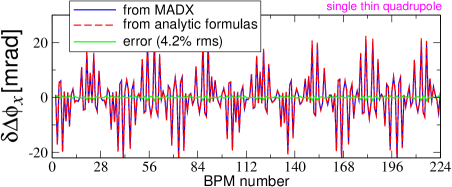
Figure 5: (Color) Top: Simulated horizontal BPM phase advance shift induced by a single thin quadrupole of the old ESRF storage ring as computed by MADX and via Eqs. (45)-(48). The rms error is of about 0.4 mrad ($4.2\%$ in relative terms). Bottom: When second-order terms are added to the above formulas the errors reduces to 0.02 mrad (i.e. $0.3\%$).

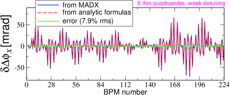
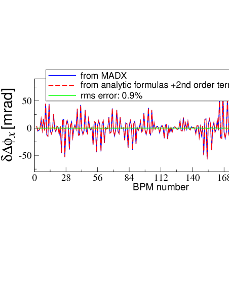
Figure 6: (Color) Top: Simulated horizontal BPM phase advance shift induced by six thin quadrupoles of the old ESRF storage ring generating a weak detuning $\Delta Q_{x}\simeq 1.5\times 10^{-4}$ as computed by MADX and via Eqs. (45)-(48). The rms error is of about 1.7 mrad ($7.9\%$ in relative terms). Bottom: When second-order terms are added to the above formulas the errors reduces to 0.2 mrad (i.e. $0.9\%$).

Eqs. (45)-(48) and more generally the linear response of the phase advance shift against the integrated quadrupole strength $\delta K_{1}$ have been tested against the actual values computed at the BPMs by MADX for the lattice of the old ESRF storage ring.
First, the simplest case with a single, thin quadrupole error has been analyzed. Results for the horizontal BPM phase advance shifts are shown in the top plot of Fig. 5 (similar plots and results are obtained in the vertical plane): The rms relative error of Eqs. (45)-(48) is of about $4.2\%$. The sizable tune shift induced by this quadrupole, $\Delta Q_{x}\simeq-2.4\times 10^{-3}$ and the non-negligible rms error suggest to seek for second-order terms $\propto\delta K_{1}^{2}$: This corresponds to keep all terms proportional to $f_{2000}^{2}$ in the various truncations and approximation made to derive Eqs. (45) and to include second-order RDTs following the procedure described in Ref. Andrea-arxiv . Handy formulas cannot be provided in this case and this correction needs to be computed numerically from the C-S parameters and first-order RDTs and Hamiltonian terms. The bottom plot of Fig. 5 shows indeed how second-order terms efficiently account for most of the initial error, the latter dropping to $0.3\%$.
A second numerical test was carried out by introducing six thin quadrupole errors generating a weak tune shift of $\Delta Q_{x}\simeq 1.5\times 10^{-4}$. The linear response of Eqs. (45)-(48) can predict the BPM phase advance shift up to $7.9\%$ rms only (see top plot of Fig. 6). Most of this error stems from second-order terms, the error going below $1\%$ when these are included (bottom plot of Fig. 6). Second and higher order terms are generated by non-zero detuning terms (negligible in this example) and by cross-terms between the several quadrupole errors.
To confirm this point, a third simulation was run with the same six quadrupole errors where one quadrupole only was changed to generate a large tune shift $\Delta Q_{x}\simeq-1.4\times 10^{-2}$. As expected, the linear dependence of the phase advance shift on the quadrupole errors of Eq.(48) is by far less accurate, as shown in the top plot of Fig. 7: The rms error reaches almost $22\%$. Second-order terms help reduce the discrepancy to less than $7\%$ (bottom plot in the same figure), though suggesting that even higher-order terms play a role in this (unrealistic) example.
An additional source of second and higher-order terms that may spoil the linear analysis of Eq.(48) is represented by betatron coupling. A fourth simulation was launched with the same 6 thin quadrupole errors of Fig. 6 (with negligible tune shift) and additional nine thin skew quadrupoles generating a large ratio between the two transverse equilibrium emittances of $\mathscr{E}_{y}/\mathscr{E}_{x}=1\%$ (The old ESRF storage ring usually operated at a ratio close to $0.1\%$). Betatron coupling decreases the accuracy of Fig. 6 from $7.9\%$ to $15.5\%$ rms, as illustrated by the top plot of Fig. 8. When second-order terms are taken into account the rms error lessens to $3.6\%$.
Simulations with errors in thick quadrupoles (not shown here) revealed a general decrease of the predictive and correcting power of Eqs. (45)-(48). In order to account for the variation of the C-S parameters across the quadrupoles, the following substitutions can be made in Eq. (45)

$$\begin{aligned} \beta_{m}\sin{(2\tau_{mj})}\hskip 1.42262pt&\longrightarrow\hskip 1.42262ptI_{S,mj}\\ \beta_{m}\sin{(2\tau_{mw})}\hskip 1.42262pt&\longrightarrow\hskip 1.42262ptI_{S,mw}\\ \end{aligned}\quad,$$ (49)

where the integrals $I_{S,mj}$ and $I_{S,mw}$ are evaluated via Eq. (548). The labels $j$ and $w$ denote here BPMs which are assumed to be of zero length.

The above numerical studies suggest some precautions need to taken when using the BPM phase advance errors and the linear system of Eq. (48) (regardless the way the linear response $\mathbf{P}$ is computed) to infer focusing lattice errors. As far as the old ESRF storage ring is concerned, when pseudo-inverting Eq. (48), an intrinsic accuracy as large as $4\%$ is to be expected even in the most ideal and simple case. Any fit of quadrupole errors leading to a fit error below this value is to be considered as unreliable. The accuracy deteriorates in the presence of large betatron coupling and detuning. Preliminary simulations shall then be run with the expected lattice configuration and errors, in order to estimate the level of accuracy expected when fitting quadrupole errors via Eq. (48).

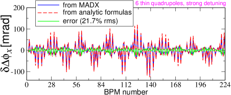
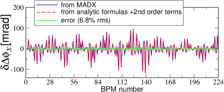
Figure 7: (Color) Top: The same six thin quadrupoles of Fig. 6 are modified so to induce a strong detuning $\Delta Q_{x}\simeq-1.4\times 10^{-2}$ and the agreement between MADX and Eqs. (45)-(48) worsens to 7.3 mrad rms (or $21.7\%$ in relative terms). Bottom: When second-order terms are added to the above formulas the rms error reduces to 2.3 mrad (i.e. $6.8\%$).

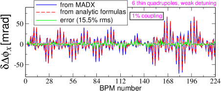
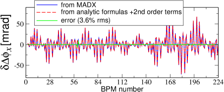
Figure 8: (Color) Top: Nine skew quadrupoles generating an emittance ratio $\mathscr{E}_{y}/\mathscr{E}_{x}=1\%$ are added to the same six thin quadrupoles of Fig. 6 and the agreement between MADX and Eqs. (45)-(48) deteriorates to 3.2 mrad rms (or $15.5\%$ in relative terms). Bottom: second-order terms reduce the rms error to 0.7 mrad (i.e. $3.6\%$).

VI Analytic formulas for the evaluation of chromatic functions from lattice parameters

In order to derive Eq. (41), an off-momentum Hamiltonian formalism is used in Appendix B. With the same algebra other chromatic functions have been derived. They represent an extension of existing formulas for an ideal lattice of Ref. Bengtsson to a more general case including magnet errors and tilts from dipoles up to sextupoles. Possible use of these equations is discussed in Sec. VII.

As for the linear dispersion, the edge focusing provided by nonzero dipole pole-face angles is not included in the lattice representation, the magnetic modelling being based on the multipolar expansion of Eq. (24).

VI.1 Linear chromaticity

Off-energy particles experience the nominal focusing forces provided by quadrupoles and an additional one induced by the quadrupolar feed-down generated by the non-zero dispersive orbit at the sextupoles. The main consequence for such particles is a shift of their betatron tune, $Q(\delta)=Q+Q^{\prime}\delta$, where $Q^{\prime}$ is the linear chromaticity. The latter reads

$$\begin{array}[]{l}\displaystyle Q_{x}^{\prime}=-\displaystyle\frac{1}{4\pi}\sum\limits_{m=1}^{M}\left(K_{m,1}-K_{m,2}D_{m,x}+J_{m,2}D_{m,y}\right)\beta_{m,x}\ ,\vspace{ 1.5mm}\\ \displaystyle Q_{y}^{\prime}=+\displaystyle\frac{1}{4\pi}\sum\limits_{m=1}^{M}\left(K_{m,1}-K_{m,2}D_{m,x}+J_{m,2}D_{m,y}\right)\beta_{m,y}\ .\end{array}$$ (52)

As expected, both quantities do not depend on the longitudinal position (or the betatron phase) and differ only by the sign and the beta functions, the argument within the parenthesis being the same in both planes. This indeed represent the effective quadrupole forces experienced by off-energy particles. The above relations require some comments. First, textbook formulas are retrieved when removing either vertical dispersion $D_{m,y}$ or the skew sextupole strengths $J_{2}$. Second, skew quadrupole fields $J_{1}$ do not influence explicitly linear chromaticity, at least to first order. Betatron coupling enters only indirectly in Eq. (52) through vertical dispersion $D_{y}$. Beta and dispersion functions in Eq. (52) refer to the lattice model including focusing errors, if any.

In order to account for the variation of the beta function across quadrupoles, the following substitution can be made

$$\beta_{m}\hskip 1.42262pt \longrightarrow\hskip 1.42262ptI_{\beta,m}\quad,\hskip 28.45274pt\beta_{m}D_{m}\hskip 1.42262pt \longrightarrow\hskip 1.42262ptL_{\beta,D,m}\quad,$$ (53)

where $I_{\beta,m}$ is defined in Eq. (547) and $L_{\beta,D,m}$ is evaluated in Eq. (607) (sextupoles are modelled as drifts).

VI.2 Chromatic beating

Another consequence of the additional focusing experienced by off-momentum particles is a modulation of beta functions. Even an ideal lattice with no focusing error (i.e. no on-momentum geometric beta-beating) is unavoidably subjected to an energy-dependent modulation of the betas and hence to the corresponding half-integer resonance. This chromatic beating can be simply defined as the derivative of the beta function with respect to $\delta$, since

$$\beta(\delta)=\beta+\frac{\partial\beta}{\partial\delta}\bigg{|}_{\delta=0}\delta+(\delta^{2})\ .$$ (54)

In practice it is more convenient to express the beating as the normalized derivative

$$\tilde{\beta}^{\prime}=\frac{1}{\beta}\frac{\partial\beta}{\partial\delta}\bigg{|}_{\delta=0}\ .$$ (55)

This quantity has the great advantage of being a dimensionless observable which is not affected by BPM calibration errors. In Appendix B the following expressions are derived for the chromatic beating in the two transverse planes:

$$\begin{array}[]{l}\displaystyle\tilde{\beta}_{x}^{\prime}(j)\simeq+\Big{\{}\sum_{m=1}^{M}\left(K_{m,1}-K_{m,2}D_{m,x}+J_{m,2}D_{m,y}\right)\times\\ \displaystyle\hskip 73.97733pt\beta_{m,x}\cos{(2\tau_{x,mj})}\Big{\}}\frac{1}{2\sin{(2\pi Q_{x})}}-1\\ \\ \displaystyle\tilde{\beta}_{y}^{\prime}(j)\simeq-\Big{\{}\sum_{m=1}^{M}\left(K_{m,1}-K_{m,2}D_{m,x}+J_{m,2}D_{m,y}\right)\times\\ \displaystyle\hskip 73.97733pt\beta_{m,y}\cos{(2\tau_{y,mj})}\Big{\}}\frac{1}{2\sin{(2\pi Q_{y})}}-1\end{array}\quad,$$ (61)

where the shifted phase advance $\tau_{mj}=\Delta\phi_{mj}-\pi Q$ is the same of Eq. (33) and the phase advance $\Delta\phi_{mj}$ is to be computed according to Eq. (25). Note that the argument within the above parentheses is the same in both planes and equal to the one of Eq. (52), as it represents the effective quadrupole strengths experienced by off-energy particles. The structure of the above summations, which is responsible for the modulation of the beating along the ring, is also identical to the one of the formulas for the geometric beta beating induced by focusing errors Andrea-Linear-arxiv . It is worthwhile noticing that the above expressions differ from the ones found in the literature Luo-chrom ; Tevatron for the presence of the $-1$ (or $-\beta$ if the un-normalized derivative is used) in the r.h.s., which stems from the invariant. This term does not affect the construction of a response matrix to correct the chromatic beating with sextupoles, since it cancels out. Similarly, it does not affect the evaluation of the difference between the model and the measured chromatic beating, provided that the former is computed by an optics code, such as MADX or PTC, which includes automatically this term.

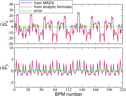
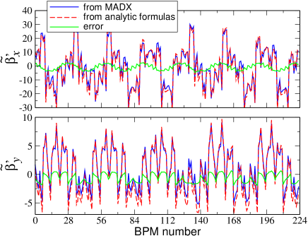
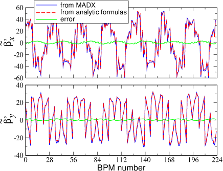
Figure 9: (Color) Examples of chromatic beating computed by MADX-PTC and by Eq. (61). Top: The ideal lattice of the old ESRF storage ring with no skew sextupole is used and the rms error of the analytic formulas is of about 0.10 ($6\%$), mostly in the vertical plane. Center: A strong skew sextupole and a tilted dipole are introduced in the lattice model to enhance the contribution of the $J_{m,2}D_{m,y}$ term in Eq. (61), leading to larger chromatic beating and greater error of the analytic formula ($22\%$ rms). Bottom: The latter lattice model is further modified by removing the edge focusing in the dipoles, which increases even more the vertical chromatic beating while reducing the error of Eq. (61) to below $5\%$.

The robustness of Eq. (61) was tested numerically against the values computed by MADX via the

TC_twiss  module for several configurations.
The ideal lattice of the old ESRF storage ring  including
the edge focusing in the bending magnets (not included
explicitly in the analytic formulas) was used for a
first test, whose results are reported in the top two plots
of Fig.~\ref{fig_ChromBeat1}: The agreement is of about $6\%$
rms, mostly in the vertical plane (it is of $0.3\%$
horizontally). The chromatic beating is not periodic
because of one insertion optics with a non-standard
quadrupole and sextupole layout (around the B

M number 135). In order to asses the validity of the $J_{m,2}D_{m,y}$ term, a strong skew sextupole and a large vertical deflection were then introduced into the model so to generate a sizable vertical dispersion and alter significantly the chromatic beating compared to the nominal lattice. The result of this test is shown in the central two plots of Fig. 9: The beating is indeed rather different, especially in the vertical plane, and Eq. (61) could reproduce this change quite well, even though the relative error increases to about $22\%$ rms in this example. This test and the fact the this contribution is of second order (in $J_{m,2}D_{m,y}$ both vertical dispersion and skew sextupole field components are orders of magnitude lower than the horizontal dispersion and normal sextupole strengths of $K_{m,2}D_{m,x}$) suggest that Eq. (61) is not suitable for the evaluation of skew sextupole field components in real machines. In the attempt of better understanding the source of such discrepancy, a third test was carried out with the same two strong magnets, though removing the edge focusing in the dipoles (without retuning the baseline lattice). The chromatic beating of this unrealistic model changed completely, as demonstrated by the bottom two plots of Fig. 9 and the accuracy of Eq. (61) improved greatly, reaching an rms error of $5\%$, this time mainly in the horizontal plane (it is of $3.6\%$ for $\tilde{\beta}_{y}^{\prime}$).

As for the previous formulas, the accuracy of Eq. (61) can be improved by accounting for the variation of the C-S parameters and dispersion across the magnets, i.e. replacing

$$\begin{aligned} \beta_{m}\cos{(2\tau_{mj})}\hskip 1.42262pt&\longrightarrow\hskip 1.42262ptI_{C,mj}\quad,\\ D_{m,q}\beta_{m,p}\cos{(2\tau_{p,mj})}\hskip 1.42262pt&\longrightarrow\hskip 1.42262ptL_{C_{p},D_{q},mj}\ ,\ (p,q=x,y)\quad,\quad\end{aligned}$$ (62)

where the integral $I_{C,mj}$ is evaluated via Eq. (548) and $L_{C_{p},D_{q},mj}$ is computed in Eq. (611). In both case, the transport over a thick sextupole is modelled as a drift space.

VI.3 chromatic phase advance shift

Quadrupole errors induce a betatron phase shift to particles with nominal energy. When going off momentum the additional focusing provided by the off-axis closed orbit across sextupoles generate a similar chromatic phase shift. In Appendix B the following expressions are derived for the derivative of the phase advance shift with respect to $\delta$

$$\Delta\phi_{x,wj}^{\prime} = \frac{\partial\Delta\phi_{x,wj}}{\partial\delta}\Bigg{|}_{\delta=0}$$

$$\simeq -\frac{1}{4}\sum_{m=1}^{M}\left(K_{m,1}-K_{m,2}D_{m,x}+J_{m,2}D_{m,y}\right)\beta_{m,x}$$

$$\hskip 34.1433pt\times\Big{\{}2\Big{[}\Pi(m,j)-\Pi(m,w)+\Pi(j,w)\Big{]}$$

$$\hskip 48.36967pt+\frac{\sin{(2\tau_{x,mj})}-\sin{(2\tau_{x,mw})}}{\sin{(2\pi Q_{x})}}\Big{\}},$$

where the functions $\Pi$ and $\tau$ are the same of Eqs. (32) and (33), respectively. The chromatic shift in the vertical plane reads

$$\Delta\phi_{y,wj}^{\prime} = \frac{\partial\Delta\phi_{y,wj}}{\partial\delta}\Bigg{|}_{\delta=0}$$

$$\simeq +\frac{1}{4}\sum_{m=1}^{M}\left(K_{m,1}-K_{m,2}D_{m,x}+J_{m,2}D_{m,y}\right)\beta_{m,y}$$

$$\hskip 34.1433pt\times\Big{\{}2\Big{[}\Pi(m,j)-\Pi(m,w)+\Pi(j,w)\Big{]}$$

$$\hskip 48.36967pt+\frac{\sin{(2\tau_{y,mj})}-\sin{(2\tau_{y,mw})}}{\sin{(2\pi Q_{x})}}\Big{\}}.$$

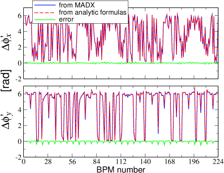
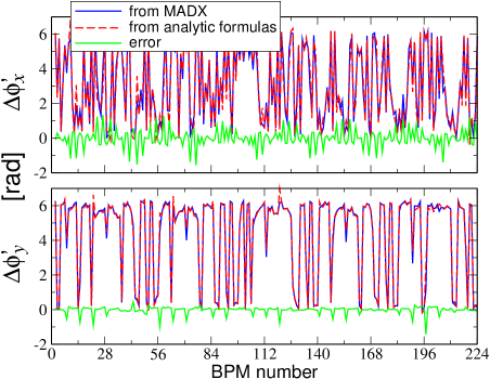
Figure 10: (Color) Examples of comparison between the chromatic phase advance shift computed by Eqs. (VI.3)-(VI.3) and MADX-PTC. Top two plots: ideal lattice of the old ESRF storage ring without the dipole edge focusing. Center two plots: same lattice, after reintroducing the nominal edge focusing in the bending magnets and adding 4 strong skew sextupoles and a tilted dipole. Bottom two plots: A typical set of linear errors (focusing and coupling) inferred from ORM measurement is added to the second lattice model.

As for the chromatic beating of Sec. VI.2 the accuracy of the above formulas was tested numerically against the same quantities computed by MADX-PTC for several configurations. In Fig. 10 the comparison with three different lattice models is reported. In the first two plots, $\Delta\phi_{wj}^{\prime}$ is evaluated for the ideal lattice of the old ESRF storage ring without the dipole edge focusing, resulting in an excellent agreement within $0.5\%$ rms. In the second pair of plots, the phase advance shift is calculated from the same lattice, after reintroducing the nominal edge focusing in the bending magnets and including 4 strong skew sextupoles and a 100 mrad tilt in a dipole so to enhance the term $J_{m,2}D_{m,y}$ in Eqs. (VI.3)-(VI.3): The agreement is worse, at about $2\%$ and $5\%$ rms in the horizontal and vertical planes, respectively. The last two graphs correspond to the later lattice model with a typical set of linear errors (focusing and coupling) inferred from ORM measurement. The presence of betatron coupling which excites higher-order terms not included in the above formulas (of which more in Sec. VI.6) worsen the predictive power of the analytic formulas, with rms errors of about $20\%$ and $9\%$ in the two planes.

Once again, the accuracy of Eqs. (VI.3)-(VI.3) can be improved by accounting for the variation of the C-S parameters and dispersion across the magnets with the following substitutions

$$\begin{aligned} \beta_{m}\hskip 1.42262pt&\longrightarrow\hskip 1.42262ptI_{\beta,m}\quad,\\ \beta_{m}\sin{(2\tau_{mj})}\hskip 1.42262pt&\longrightarrow\hskip 1.42262ptI_{S,mj}\quad,\\ D_{m,q}\beta_{m,p}\sin{(2\tau_{p,mj})}\hskip 1.42262pt&\longrightarrow\hskip 1.42262ptL_{S_{p},D_{q},mj}\ ,\ (p,q=x,y)\quad,\quad\end{aligned}$$ (65)

where the integrals $I_{\beta,m}$, $I_{S,mj}$ and $L_{S_{p},D_{q},mj}$ are evaluated via Eqs. (547), (548) and Eq. (611), respectively.

VI.4 Second-order dispersion

The linear dependence of the closed orbit on the energy (i.e. the dispersion function) is a function of mainly the bending magnets and the on-momentum linear optics, as demonstrated by Eq. (41). At larger energy deviation the quadratic dependence of the orbit on $\delta$ needs to be taken into account. This corresponds to the derivative of the dispersion function with respect to $\delta$, namely

$$D_{x}^{\prime}=\frac{\partial^{2}x_{co}}{\partial\delta^{2}}=\frac{\partial D_{x}}{\partial\delta}\quad.$$ (66)

The same definition applies to the vertical plane. Some authors Bengtsson define the second-order dispersion from the Taylor expansion in $\delta$, hence introducing a factor $1/2$. In order to follow the MADX-PTC nomenclature, Eq. (66) is used in this paper to define $D^{\prime}$. Conversely to the linear dispersion, $D^{\prime}$ depends on the modified off-momentum optics as well as on the dipolar feed-down from quadrupoles and sextupoles. Like for the chromatic beating, it is of interest to evaluate the dispersion normalized to the square root of the beta function, in order to make this observable independent of any possible BPM calibration error. In Appendix B the one-turn map of Eq. (29) is used along with the computation of the Hamiltonian terms proportional to $\delta^{2}$ to derive the following analytic relations

$$\left\{\begin{aligned} \tilde{D}_{x}^{\prime}(j)&=\frac{D_{x}^{\prime}(j)}{\sqrt{\beta_{x}(j)}}=\Re\left\{\tilde{d}_{x,-}^{\prime}(j)\right\}\\ \tilde{D}_{y}^{\prime}(j)&=\frac{D_{y}^{\prime}(j)}{\sqrt{\beta_{y}(j)}}=\Re\left\{\tilde{d}_{y,-}^{\prime}(j)\right\}\end{aligned}\right.\quad,$$ (67)

where $\tilde{d}_{x,-}^{\prime}=\tilde{D}_{x}-i\tilde{D}_{x}^{\prime}$ and $\tilde{d}_{y,-}^{\prime}=\tilde{D}_{y}-i\tilde{D}_{y}^{\prime}$ are the first and third elements of the complex C-S dispersion vector $\vec{d}=(\tilde{d}_{x,-},\tilde{d}_{x,+},\tilde{d}_{y,-},\tilde{d}_{y,+})^{T}$. The latter reads

$$\vec{d}^{\prime}(j)\simeq\mathbf{B}_{j}^{-1}\sum_{m=1}^{M}\left\{\frac{e^{i\mathbf{\Delta\phi}_{mj}}}{1-e^{i\mathbf{Q}}}\mathbf{B}_{m}\ 4i\left(\begin{array}[]{r}h_{m,10002}\\ -h_{m,10002}\\ h_{m,00102}\\ -h_{m,00102}\end{array}\right)\right\}\ ,\ \qquad$$ (72)

where the sum extends over all (normal and skew) $M$ dipoles, quadrupoles and sextupoles along the ring, whereas the RDT matrices $\mathbf{B}_{j}^{-1}$ and $\mathbf{B}_{m}$ are the same of Eq. (28), and the Hamiltonian coefficients are

$$\left\{\begin{aligned} h_{m,10002}&=\frac{\sqrt{\beta_{m,x}}}{2}\bigg{[}-K_{m,0}-J_{m,1}D_{m,y}+K_{m,1}D_{m,x}\\ &\hskip 2.84526pt-\frac{1}{2}K_{m,2}\left(D_{m,x}^{2}-D_{m,y}^{2}\right)+J_{m,2}D_{m,x}D_{m,y}\bigg{]}\\ h_{m,00102}&=\frac{\sqrt{\beta_{m,y}}}{2}\bigg{[}\ \ J_{m,0}-J_{m,1}D_{m,x}-K_{m,1}D_{m,y}\\ &\hskip 2.84526pt+\frac{1}{2}J_{m,2}\left(D_{m,x}^{2}-D_{m,y}^{2}\right)+K_{m,2}D_{m,x}D_{m,y}\bigg{]}\end{aligned}\right.\quad.$$

(73)

The calculation of the second-order dispersion requires hence the preliminary evaluation of the coupling RDTs in order to infer the $\mathbf{B}$ matrices. Focusing errors are to be included into the linear model to evaluate the C-S parameters and the linear dispersion, so to have $f_{2000}=f_{0020}=0$ anywhere along the ring and to compute the above Hamiltonian coefficients more accurately. The calculation simplifies greatly in the absence of linear coupling and tilted magnets, i.e. with $\mathbf{B}_{m}=\mathbf{B}_{j}^{-1}=\mathbf{I}$, $D_{m,y}=0$, $J_{m,0}=J_{m,1}=J_{m,2}=0$ and hence $h_{m,00102}=h_{m,00012}=0$:

$$\left\{\begin{aligned} \displaystyle\tilde{D}_{x}^{\prime}(j)&=4\Re\left\{\frac{e^{-i\Delta\phi_{x,mj}}}{1-e^{i2\pi Q_{x}}}i\ h_{m,01002}\right\}\\ \tilde{D}_{y}^{\prime}&=0\end{aligned}\right.\ .\qquad$$ (74)

The ideal second-order horizontal dispersion then reads

$$\tilde{D}_{x}^{\prime}(j) = \frac{1}{\sin{(\pi Q_{x})}}\sum_{m=1}^{M}\Big{[}-K_{m,0}+K_{m,1}D_{m,x}$$ (75)

$$\hskip 14.22636pt-\frac{1}{2}K_{m,2}D_{m,x}^{2}\Big{]}\sqrt{\beta_{m,x}}\cos{(\Delta\phi_{x,mj}-\pi Q_{x})}$$

$$= -2\tilde{D}_{x}(j)+\frac{1}{\sin{(\pi Q_{x})}}\sum_{m=1}^{M}\left[K_{m,1}-\frac{1}{2}K_{m,2}D_{m,x}\right]$$

$$\hskip 14.22636pt\times D_{m,x}\sqrt{\beta_{m,x}}\cos{(\Delta\phi_{x,mj}-\pi Q_{x})}\quad,$$

corresponding to Eq.(112) of Ref. Bengtsson multiplied by a factor two. In the above equation, the linear dispersion $D_{x}(j)$ of Eq. (41) has been extracted from the summation. As usual, the phase advance $\Delta\phi_{mj}$ is to be computed as in Eq. (25). If the mere difference between the two betatron phases at the positions $m$ and $j$ is used, the absolute value $|\Delta\phi_{x,mj}|$ shall then be used, as done in textbooks. $\tau_{x,mj}=\Delta\phi_{x,mj}-\pi Q_{x}$ has been omitted here to ease the comparison with the standard formula. For a lattice with errors the more general Eqs. (67)-(73) shall be used and numerically evaluated.

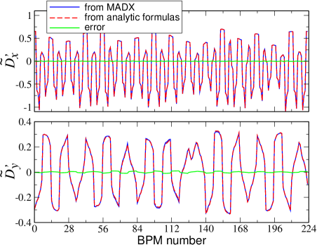
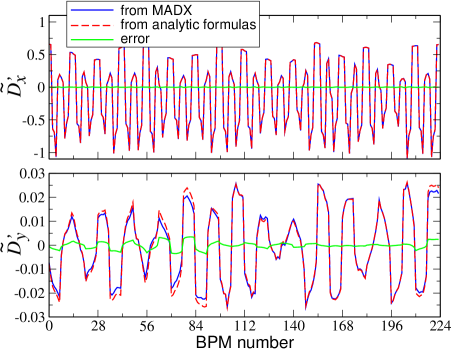
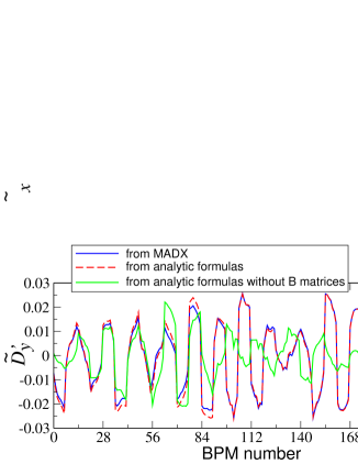
Figure 11: (Color) Examples of second-order dispersion computed via Eqs. (67)-(73) and by MADX-PTC. Top plots: typical linear lattice errors inferred from ORM measurements are included into the model of the old ESRF storage ring, along with two strong skew magnets, one quadrupole (to enhance coupling and vertical dispersion) and one sextupole (to have all contributions in Eq. (72) active). The analytic formulas predict $D_{x}^{\prime}$ within $5\%$, whereas the rms relative error for $D_{y}^{\prime}$ is of about $2.5\%$. Center plots: The previous two strong skew magnets are removed, providing the typical second-order dispersion of the old ESRF storage ring. The smaller $D_{y}^{\prime}$ is accompanied by a larger relative error ($10\%$). $D_{y}^{\prime}$ was also computed by removing the RDT matrices $\mathbf{B}$ in Eq. (72): The bottom plot shows how they cannot indeed be ignored in the evaluation of $D_{y}^{\prime}$.

Once again, the accuracy of the above formulas was tested numerically against the second-order dispersion computed by MADX-PTC for several configurations, out of which two examples are reported here. First, the lattice of the old ESRF storage ring including the edge focusing in the bending magnets (not included explicitly in the analytic formulas), as well as typical linear lattice errors (beta beating and betatron coupling) inferred from ORM measurements, was used along with one strong skew quadrupole and one skew sextupole, so to have all terms in the square brackets of Eq. (73) active. The second-order dispersion predicted by Eqs. (67)-(73) is compared to the one computed by MADX-PTC in the top plots of Fig. 11: The agreement is of about $5\%$ rms for $D_{x}^{\prime}$ and $2.5\%$ for $D_{y}^{\prime}$. In the center plots of the same figure the comparison refers to the same lattice without the strong skew quadrupole and sextupole, hence representing a typical operational scenario for the old ESRF storage ring. While $D_{x}^{\prime}$ is weakly altered (as it is dominated by the main bending magnets via $h_{m,10002}$ of Eq. (73) and the rms relative errors remains at the $5\%$ level, the derivative of the vertical dispersion is much smaller and the relative rms errors increases to about $10\%$. In order to asses the weight of the RDT matrices $\mathbf{B}$, $D_{y}^{\prime}$ was also calculated by replacing them with the identity matrix $\mathbf{I}$. The bottom plot of Fig. 11 shows how they are indeed an essential ingredient in the correct evaluation of $D_{y}^{\prime}$.

The usual thick-magnet correction to account for the variation of C-S parameters and dispersion across magnets can be in principle carried out also here, though only for the ideal horizontal dispersion of Eq. (75), by following the same procedure described in Section C. For the more general formulas Eqs. (67)-(73) a different approach needs to be defined.

VI.5 Chromatic coupling

Betatron coupling between the two transverse planes is generated by tilted quadrupoles, and non-zero vertical closed orbit inside sextupole magnets, whose feed-down field is of the skew-quadrupole type. Betatron coupling induces some vertical dispersion, on top of the one generated by any source of vertical deflection along the ring. When going off momentum, vertical dispersion adds an additional vertical beam displacement across the sextupoles, hence generating a new chromatic coupling. If skew sextupole fields are also present, the horizontal displacements induced by the natural horizontal dispersion contribute also to coupling. Betatron coupling is completely described by the two RDTs $f_{1001}$ and $f_{1010}$. Hence, in order to describe the linear dependence of betatron coupling on the energy offset, i.e. chromatic coupling, it is natural to look for analytic formulas for the derivative of the two RDTs with respect to $\delta$,

$$f_{10011}(j)=\frac{\partial f_{1001}(j)}{\partial\delta}\Bigg{|}_{\delta=0},\ f_{10101}(j)=\frac{\partial f_{1010}(j)}{\partial\delta}\Bigg{|}_{\delta=0}.\qquad\quad$$ (76)

In Appendix B it is shown how the effective coupling terms experienced by off-energy particles is represented by the Hamiltonian coefficients $h_{m,10011}=h_{m,10101}$ which depend linearly on skew quadrupoles, sextupoles (both normal and skew) and dispersion, according to

$$h_{m,10011}=-\frac{\sqrt{\beta_{m,x}\beta_{m,y}}}{4}\left(J_{m,1}-K_{m,2}D_{m,y}-J_{m,2}D_{m,x}\right).$$

(77)

Chromatic coupling is then described by the following functions

$$\begin{aligned} f_{10011}(j)&\simeq F_{10011}(j,J_{1})+\frac{\sum\limits_{m=1}^{M}h_{m,10011}e^{i(\Delta\phi_{x,mj}-\Delta\phi_{y,mj})}}{1-e^{2\pi i(Q_{x}-Q_{y})}},\\ f_{10101}(j)&\simeq F_{10101}(j,J_{1})+\frac{\sum\limits_{m=1}^{M}h_{m,10101}e^{i(\Delta\phi_{x,mj}+\Delta\phi_{y,mj})}}{1-e^{2\pi i(Q_{x}+Q_{y})}},\end{aligned}$$

(78)

where $F_{10011}$ and $F_{10101}$ are defined in Eq. (452) and depend mainly on skew quadrupole fields, and weakly on sextupole strengths, and the sum runs over all skew quadrupoles and sextupoles (both normal and skew) present in the machine. As usual, the phase advance $\Delta\phi_{mj}$ is to be computed as in Eq. (25). The remainder in Eq. (78) is proportional to $J_{1}^{2}$. MADX-PTC does not compute directly the chromatic coupling RDTs. In order to test Eq. (78) they are then computed from simulated off-energy single-particle tracking data and the harmonic analysis, as done in Ref. prstab_coup . The derivative is then numerically computed from two sets of RDTs at $\delta=\pm 10^{-3}$. In the first test, the ideal lattice of the old ESRF storage ring is used with one tilted bending magnet (to generate vertical dispersion) and one skew sextupole, though no skew quadrupole. By doing so, $f_{1001}=f_{1010}=F_{10011}=F_{10101}=0$ around the ring and the Hamiltonian coefficient of Eq. (77) contains only the coefficient $(K_{m,2}D_{m,y}-J_{m,2}D_{m,x})$ with no higher-order terms proportional to $J_{1}^{2}$ corrupting Eq. (78). This test is important in assessing whether this equation can be effectively used to compute a response matrix to correct chromatic coupling with skew sextupoles. Results are shown in Fig. 12, where the real and imaginary parts of the $f_{10011}$ and $f_{10101}$ are displayed from tracking and from Eq. (78): The agreement is well within $2\%$ rms. A second test is instead performed by removing the tilted bending magnet and the skew sextupole, after including a typical set of linear lattice errors (including skew quadrupole fields) obtained from ORM measurements. In this case, chromatic coupling is dominated by $F_{10011}$ and $F_{10101}$ along with the skew quadrupole term in $h_{m,10011}$ of Eq. (77) and the higher-order terms are no longer zero. $F_{10011}$ and $F_{10101}$ are also computed with a further numerical approximation of Eq. (416). Results are reported in Fig. 13, revealing a much worse agreement, of about $20\%$ rms, mostly for the sum RDT $f_{10101}$. Even if this test shows an intrinsic limitation in the capability of Eq. (78) in reproducing the real chromatic coupling, the first simulation shows how it can be effective in its correction by using skew sextupoles only, once skew quadrupoles are optimized to minimize the (on-momentum) betatron coupling.

     

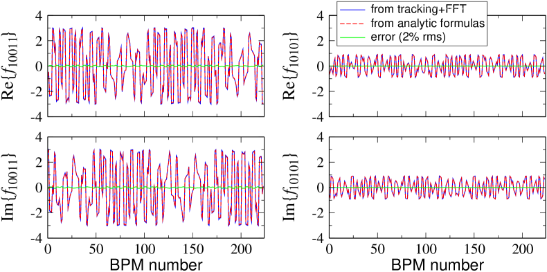
Figure 12: (Color) Chromatic coupling, expressed by the chromatic RDTs $f_{10011}$ and $f_{10101}$ for the ideal old ESRF lattice with one vertical bending magnet and one skew sextupole. The functions computed from off-energy single-particle tracking and the harmonic analysis of Ref. prstab_coup are in blue, whereas the dashed red curves refer to those evaluated from Eq. (78). Even in the absence of geometric betatron coupling ($f_{1001}=f_{1010}=F_{10011}=F_{10101}=0$ along the ring), the sextupoles (normal and skew) couple with the dispersion functions (both horizontal and vertical) to generate a linear coupling for all off-momentum particles.

     

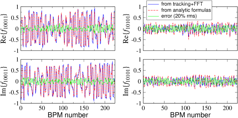
Figure 13: (Color) ) Chromatic coupling, expressed by the chromatic RDTs $f_{10011}$ and $f_{10101}$ for the ESRF lattice with a set of lattice errors (focusing and betatron coupling) inferred from beam-based measurements. The functions computed from off-energy single-particle tracking and the harmonic analysis of Ref. prstab_coup are in blue, whereas the dashed red curves refer to those evaluated from Eq. (78). Conversely to Fig. 12, chromatic coupling is generated here by the non-zero geometric betatron coupling. The agreement between tracking and the analytic predictions of Eq. (78) is worse than in Fig. 12, since there is a non-zero second-order Hamiltonian contribution (see Sec. VI.6) stemming from skew quadrupoles.

VI.6 Impact of higher-order Hamiltonian terms on the chromatic functions

In evaluating the robustness of Eq. (45) it has been observed that second-order terms account for a large fraction of its error. This is true for all other observables. Nonlinear contributions from magnet strengths $K_{n}$ and $J_{n}$ to these observables originate from a series of truncations and approximations which remove terms proportional to powers higher than 1 of the RDTs. Moreover if focusing errors are not included in the model, betatron coupling is present in the lattice and linear chromaticity differs from zero, there is an additional contribution to the linear chromatic functions stemming from cross-product between Hamiltonian terms. The procedure for their (numerical) evaluation is presented in Sec. B.8 of Appendix B.

VII Linear analysis of off-momentum ORM for the evaluation of a sextupolar lattice model

Linear dispersion and on-momentum ORM are routinely measured and used to fit linear lattice errors by pseudo-inverting the two systems of Eqs. (16)-(22), where the two response matrices $\mathbf{N}$ and $\mathbf{S}$ can be either obtained by simulating the measurement (slower, but more accurate) or analytically computed from the equations presented in Sec. IV (quicker, but less precise).

The same approach can be extended to off-momentum ORM and second-order dispersion $D^{\prime}$. Indeed, the off-axis orbit across sextupoles generated by the energy offset via the linear dispersion generates quadrupole feed-down field (which is linear in the sextupole strengths) altering both the linear optics (and hence the ORM) and dispersion. How strong, and hence observable, is this effect depends mainly on the dispersion function at the sextupoles: It is then suitable for chromatic sextupoles, less so for the harmonic ones. The systems of Eqs. (16)-(22) can be extended to the case with $\delta\neq 0$ according to

$$\begin{array}[]{c}\left(\begin{array}[]{c}\delta\vec{O}^{(xx)}\\ \delta\vec{O}^{(yy)}\\ \delta\vec{D}_{x}\end{array}\right)_{\delta\neq 0}=\mathbf{N}_{\delta}\left(\begin{array}[]{c}\delta\vec{K}_{2}\\ \delta\vec{K}_{1}\\ \delta\vec{K}_{0}\end{array}\right)\ ,\vspace{2mm}\\ \left(\begin{array}[]{c}\delta\vec{O}^{(xy)}\\ \delta\vec{O}^{(yx)}\\ \delta\vec{D}_{y}\end{array}\right)_{\delta\neq 0}=\mathbf{S}_{\delta}\left(\begin{array}[]{c}\vec{J}_{2}\\ \vec{J}_{1}\\ \vec{J}_{0}\end{array}\right)\ .\end{array}$$ (93)

$\delta\vec{K}_{2}$ and $\delta\vec{J}_{2}$ are the vectors containing the sextupole errors and tilts (represented by skew sextupole integrated strengths). $\delta{\mathbf{O}}_{\delta\neq 0}$ and $\delta\vec{D}_{\delta\neq 0}$ denote instead the deviation between the measured and the model off-energy ORM and dispersion, whereas $\mathbf{N}_{\delta}$ and $\mathbf{S}_{\delta}$ are the response matrices of Eqs. (16)-(22) including sextupole magnets and computed at a given $\delta\neq 0$. However, the linear lattice errors inferred from the on-momentum ORM and dispersion can be inserted in the model used to compute the corresponding off-momentum quantities. If the deviations $\delta{\mathbf{O}}_{\delta\neq 0}$ and $\delta\vec{D}_{\delta\neq 0}$ are then computed with respect to this modified model, the above systems simplifies to

$$\begin{array}[]{c}\left(\begin{array}[]{c}\delta\vec{O}^{(xx)}\\ \delta\vec{O}^{(yy)}\\ \delta\vec{D}_{x}\end{array}\right)_{\delta\neq 0}=\mathbf{N^{\prime}}_{\delta}\ \delta\vec{K}_{2}\ ,\vspace{2mm}\\ \left(\begin{array}[]{c}\delta\vec{O}^{(xy)}\\ \delta\vec{O}^{(yx)}\\ \delta\vec{D}_{y}\end{array}\right)_{\delta\neq 0}=\mathbf{S^{\prime}}_{\delta}\ \vec{J}_{2}\ ,\hskip 11.38109pt\end{array}$$ (102)

where both $\mathbf{N^{\prime}}_{\delta}$ and $\mathbf{S^{\prime}}_{\delta}$ are now computed from the model including the linear errors. The pseudo-inversion of these two later systems can be then used to infer an error model for the (chromatic) sextupoles. Eq. (102) may be modified by inserting weights and fixing chromaticity to the measured value in order to obtain an effective model.

Alternatively, two measurements at $\pm\delta$ of both ORM and linear dispersion can be performed. From the linear analysis of Eqs. (16)-(22), which shall include the energy offset and sextupole magnets, the linear lattice parameters ($\beta,\ f_{1001},\ f_{1010}$ and $D_{x,y}$) at the BPMs can be computed at $\pm\delta$. Their derivative with respect to $\delta$, i.e. the chromatic functions of Sec. VI, can be then evaluated:

$$\left(\begin{array}[]{c}\delta{\mathbf{O}}_{\pm\delta}\vspace{1mm}\\ \vec{D}_{\pm\delta}\end{array}\right)\Rightarrow\begin{array}[]{c}\left(\begin{array}[]{c}\vec{\beta}\vspace{1mm}\\ \vec{f}_{1001}\vspace{1mm}\\ \vec{f}_{1010}\vspace{1mm}\\ \vec{D}\end{array}\right)_{\pm\delta}\end{array}\Rightarrow\left(\begin{array}[]{c}\vec{\beta}^{\prime}\vspace{1mm}\\ \vec{f}_{10011}\vspace{1mm}\\ \vec{f}_{10101}\vspace{1mm}\\ \vec{D}^{\prime}\end{array}\right)\ .$$ (114)

The vector with the difference between measured and model chromatic functions can be expressed in terms of sextupole errors (strengths and tilts) according to

$$\left(\begin{array}[]{c}\vec{\beta}^{\prime}\\ \hskip-2.84526pt\vec{f}_{10011}\hskip-5.69054pt\vspace{1mm}\\ \hskip-2.84526pt\vec{f}_{10101}\hskip-5.69054pt\vspace{1mm}\\ \vec{D}^{\prime}\end{array}\right)^{\hskip-2.84526pt(meas)}\hskip-11.38109pt-\hskip 2.84526pt\left(\begin{array}[]{c}\vec{\beta}^{\prime}\\ \hskip-2.84526pt\vec{f}_{10011}\hskip-5.69054pt\vspace{1mm}\\ \hskip-2.84526pt\vec{f}_{10101}\hskip-5.69054pt\vspace{1mm}\\ \vec{D}^{\prime}\end{array}\right)^{\hskip-2.84526pt(mod)}\hskip-11.38109pt=\hskip 2.84526pt\mathbf{T}\left(\begin{array}[]{c}\delta\vec{K}_{2}\vspace{1mm}\\ \vec{J}_{2}\end{array}\right)\ ,$$ (125)

where the betatronic block of the response matrix $\mathbf{T}$ is computed from Eq. (61), the part corresponding to the chromatic coupling is obtained from Eqs. (77)-(78), whereas the terms for the second-order dispersion are derived from Eqs. (67)-(73). Once again, weights between the different parameters and constant chromaticity (see Eq. (52)) shall be included to the above system to obtain a realistic model. The complex chromatic RDTs $f_{10011}$ and $f_{10101}$ may be split in real and imaginary parts to preserve the linearity of the system. Interestingly, when evaluating $\mathbf{T}$ it is not necessary to include terms either constant, such as the -1 in the formulas for $\beta^{\prime}$ of Eq. (61), or independent on sextupole strengths, e.g. the complicated functions $F_{10011}$ and $F_{10101}$ in Eq. (78). The BPM chromatic phase advance shift can be also included in Eq. (125) or replace the chromatic beating. In this case the system to be pseudo-inverted would read

$$\left(\begin{array}[]{c}\Delta\vec{\phi}^{\prime}\\ \hskip-2.84526pt\vec{f}_{10011}\hskip-5.69054pt\vspace{1mm}\\ \hskip-2.84526pt\vec{f}_{10101}\hskip-5.69054pt\vspace{1mm}\\ \vec{D}^{\prime}\end{array}\right)^{\hskip-2.84526pt(meas)}\hskip-11.38109pt-\hskip 2.84526pt\left(\begin{array}[]{c}\Delta\vec{\phi}^{\prime}\\ \hskip-2.84526pt\vec{f}_{10011}\hskip-5.69054pt\vspace{1mm}\\ \hskip-2.84526pt\vec{f}_{10101}\hskip-5.69054pt\vspace{1mm}\\ \vec{D}^{\prime}\end{array}\right)^{\hskip-2.84526pt(mod)}\hskip-11.38109pt=\hskip 2.84526pt\mathbf{T^{\prime}}\left(\begin{array}[]{c}\delta\vec{K}_{2}\vspace{1mm}\\ \vec{J}_{2}\end{array}\right)\ ,$$ (136)

where the $\mathbf{T^{\prime}}$ differs from $\mathbf{T}$ for the block corresponding to the chromatic phase shift, which is computed from Eqs. (VI.3)-(VI.3).

The advantage of using the chromatic functions instead of the off-momentum ORM is that the same systems of Eqs. (125)-(136) can be defined irrespective of the measurement technique. For example, chromatic functions can be measured from the harmonic analysis of BPM turn-by-turn off-momentum data.

VIII Conclusion

Analytic formulas for the computation of the distortion of orbit response matrix (ORM) induced by quadrupole errors and rotations have been derived and tested by using the lattice model of the ESRF storage rings (old and new). An accuracy at the level of a few percent (rms) has been demonstrated. Explicit formulas for the evaluation of chromatic functions (beta beating, phase shift, coupling and second-order dispersion) were also derived. Their robustness depends largely on the suppression of higher-order terms that can be minimized by including focusing errors in the model and correcting coupling. By doing so, a chromatic sextupole error model can be inferred from the analysis of either the off-momentum ORM or the chromatic functions, the correlation being linear with the sextupole strengths and tilts.

Appendix A Derivation of the ORM response due to quadrupole errors and tilts

The standard procedure to evaluate the closed orbit distortion induced by a dipole horizontal perturbation $\Theta_{w}$ is based on the closed-orbit condition

$$\mathbf{M}{X}_{+}={X}_{-}\ ,\qquad{X}_{-}=\left(\begin{array}[]{c}x_{w}\\ p_{x,w}-\theta_{w}\end{array}\right)\ ,\quad{X}_{+}=\left(\begin{array}[]{c}x_{w}\\ p_{x,w}\end{array}\right)\ ,\quad\mathbf{M}\ \hbox{is the ideal one-turn matrix}$$ (141)

In the absence of lattice errors, the two planes are decoupled and an equivalent relation applies to the vertical plane. In the Courant-Snyder (C-S) coordinates the above system reads

$$\mathbf{R}\tilde{X}_{+}=\tilde{X}_{-}\ ,\qquad\tilde{X}_{-}=\left(\begin{array}[]{c}\tilde{x}_{w}\\ \tilde{p}_{x,w}-\sqrt{\beta_{w,x}}\Theta_{w}\end{array}\right)\ ,\quad\tilde{X}_{+}=\left(\begin{array}[]{c}\tilde{x}_{w}\\ \tilde{p}_{x,w}\end{array}\right)\ ,\quad\mathbf{R}=\left(\begin{array}[]{c c}\cos{(2\pi Q_{x})}&\sin{(2\pi Q_{x})}\\ -\sin{(2\pi Q_{x})}&\cos{(2\pi Q_{x})}\end{array}\right)\ ,\quad$$ (148)

whose solution reads

$$\left\{\begin{aligned} \displaystyle\tilde{x}_{w}&=\frac{\sqrt{\beta_{w,x}}\Theta_{w}\cos{(\pi Q_{x})}}{2\sin{(\pi Q_{x})}}\\ \tilde{p}_{x}&=\frac{\sqrt{\beta_{w,x}}\Theta_{w}}{2}\end{aligned}\right.\qquad\Rightarrow\qquad\left\{\begin{aligned} \displaystyle x_{w}&=\frac{\beta_{w,x}\Theta_{w}\cos{(\pi Q_{x})}}{2\sin{(\pi Q_{x})}}\\ p_{x}&=\frac{\Theta_{w}}{2\sin{(\pi Q_{x})}}(\sin{\pi}Q_{x}-\alpha_{x}\cos{(\pi Q_{x})})\end{aligned}\right.\quad.$$ (149)

The closed orbit at a generic location $j$ is obtained again first in the C-S coordinates, where the transport between the position $w$ and $s$ is a mere rotation by the corresponding phase advance, and then in the Cartesian ones:

$$\mathbf{R}\tilde{X}_{+}=\tilde{X}_{-}\ ,\quad\left(\begin{array}[]{c}\tilde{x}_{j}\\ \tilde{p}_{x,j}\end{array}\right)=\mathbf{R}\left(\Delta\phi_{x,wj}\right)\left(\begin{array}[]{c}\tilde{x}_{w}\\ \tilde{p}_{x,w}\end{array}\right)\quad\Rightarrow\quad\left\{\begin{aligned} \displaystyle\tilde{x}_{j}&=\frac{\sqrt{\beta_{w,x}}\Theta_{w}}{2\sin{(\pi Q_{x})}}\cos{(\Delta\phi_{x,wj}-\pi Q_{x})}\\ x_{j}&=\frac{\sqrt{\beta_{w,x}\beta_{j,x}}\Theta_{w}}{2\sin{(\pi Q_{x})}}\cos{(\Delta\phi_{x,wj}-\pi Q_{x})}\end{aligned}\right.\quad.$$ (154)

The phase advance between the BPM $j$ and the magnet $w$, $\Delta\phi_{x,wj}$, must be a positive quantity. However, if it is computed from the ideal betatron phases $\phi_{x,j}$ and $\phi_{x,w}$ with a fixed origin, it becomes negative whenever the magnet is downstream the BPM: In this case the total phase advance (i.e. over one turn) needs to be added, namely

$$\left\{\begin{aligned} &\Delta\phi_{x,wj}=(\phi_{x,j}-\phi_{x,w})\hskip 36.98866pt\ ,\ \hbox{if\ }\phi_{x,j}>\phi_{x,w}\\ &\Delta\phi_{x,wj}=(\phi_{x,j}-\phi_{x,w})+2\pi Q_{x}\ ,\ \hbox{if\ }\phi_{x,j}<\phi_{x,w}\end{aligned}\right.\ ,\ \left\{\begin{aligned} &\Delta\phi_{x,wj}-\pi Q_{x}=(\phi_{x,j}-\phi_{x,w})-\pi Q_{x}\ ,\ \hbox{if\ }\phi_{x,j}>\phi_{x,w}\\ &\Delta\phi_{x,wj}-\pi Q_{x}=(\phi_{x,j}-\phi_{x,w})+\pi Q_{x}\ ,\ \hbox{if\ }\phi_{x,j}<\phi_{x,w}\end{aligned}\right.\ .\qquad\quad$$ (155)

Even though Eq. (154) is found in the literature with $\cos{(|\Delta\phi_{x,wj}|-\pi Q_{x})}$, which smartly accounts for both cases, since $\cos{(x)}=\cos{(-x)}$, it is no longer convenient for the more general formula to be derived. Hence, the definition of $\Delta\phi_{x,wj}$ given in Eq. (155) is kept throughout the paper.

The orbit response being linear in $\Theta_{w}$, if several sources of dipole perturbations are present, a sum over $w$ shall be included in the above equations. In the vertical plane identical relations apply after substituting $x$ with $y$.

In the presence of focusing errors and linear coupling the above procedure does not apply, since the two planes are no longer decoupled, neither in the Cartesian nor in the C-S coordinates. Even including focusing errors in the model ($\delta K_{1}=0$) betatron coupling induced by skew quadrupole fields $\delta J_{1}\neq 0$ requires a more careful approach. The generalization of the C-S coordinates in the presence of betatron coupling (and nonlinearities) is represented by the normal form coordinates. As the C-S transformation absorbs the envelope modulation induced by the ideal focusing lattice and reshape the $s$-dependent elliptical phase space portraits in an invariant circle, the (non-resonant) normal form transformation absorbs focusing errors, betatron coupling and, with some precautions, lattice nonlinearities, retrieving circular orbits in phase space from the distorted curves in the original Cartesian phase space. In normal forms, the two planes are also decoupled. Such transformation is a polynomial function $F$

$$F=\sum_{n}\sum_{pqrt}^{n=p+q+r+t}{f_{pqrt}\zeta_{x,+}^{p}\zeta_{x,-}^{q}\zeta_{y,+}^{r}\zeta_{y,-}^{t}}\ ,$$ (156)

where $n$ denotes the multipole order, $f_{pqrt}$ are RDTs and $\zeta_{z,\pm}=\sqrt{2I_{z}}e^{\mp i(\psi_{z}+\psi_{z,0})}$ are the new complex normal form coordinates ($z$ stands for either $x$ or $y$), which are the decoupled and nonlinear generalization of the complex C-S complex variable $h_{z,\pm}=\tilde{z}\pm i\tilde{p}_{z}=\sqrt{2J_{z}}e^{\mp i(\phi_{z}+\phi_{z,0})}$. The equation establishing the change of coordinates in normal form at a generic point $j$ may be written in terms of Lie operators and Poisson brackets $[\ ,\ ]$

$$\vec{\zeta}_{j} = e^{:-F_{j}:}\vec{h}_{j}=\vec{h}_{j}+[-F_{j},\vec{h}_{j}]+O(F^{2})\ ,\qquad\vec{h}_{j}=e^{:F_{j}:}\vec{\zeta}_{j}=\vec{\zeta}_{j}+[F_{j},\vec{\zeta}_{j}]+O(F^{2})\ ,$$ (157)

where $\vec{h}=(h_{x,-},h_{x,+},h_{y,-},h_{y,+})^{T}$ and $\vec{\zeta}$ its equivalent in normal form, whereas $e^{::}$ denotes the Lie operator. The remainder $O(F^{2})$ contains nested Poisson Brackets and scales with the RDTs squared. The above transformations imply that to the first order in the RDTs, $F(\vec{\zeta})=F(\vec{h})+O(f^{2})$ since the two variables $\vec{\zeta}$ and $\vec{h}$ are tangent, i.e. $\vec{\zeta}=\vec{h}+O(f)$. In the presence of focusing errors and sources of betatron coupling only terms such that $p+q+r+t=2$ (i.e. normal and skew quadrupolar $\propto x^{2},\ y^{2}$ and $xy$) are to be selected in Eq. (156) in order to remove the dependence upon them in the normal forms coordinates:

$$F=f_{2000}\zeta_{x,+}^{2}+f_{2000}^{*}\zeta_{x,-}^{2}+f_{0020}\zeta_{y,+}^{2}+f_{0020}^{*}\zeta_{y,-}^{2}+f_{1001}\zeta_{x,+}\zeta_{y,-}+f_{1001}^{*}\zeta_{x,-}\zeta_{y,+}+f_{1010}\zeta_{x,+}\zeta_{y,+}+f_{1010}^{*}\zeta_{x,-}\zeta_{y,-}\ ,$$

where the relation (valid to first order only Andrea-arxiv ) $f_{pqrt}=f_{qptr}^{*}$ has been used. To first order, the RDTs at a location $j$ read Andrea-arxiv

$$f_{pqrt}(j)=\frac{\sum\limits_{m}^{M}h_{m,pqrt}e^{i[(p-q)\Delta\phi_{x,mj}+(r-t)\Delta\phi_{y,mj}]}}{1-e^{2\pi i[(p-q)Q_{x}+(r-t)Q_{y}]}}\ \ .$$ (158)

The coefficients $h_{m,pqrt}$ derive from the Hamiltonian term in the complex C-S coordinates generated by a generic magnet $m$

$$\tilde{H}_{m}=\sum_{pqrt}^{n=p+q+r+t}{h_{m,pqrt}h_{m,x,+}^{p}h_{m,x,-}^{q}h_{m,y,+}^{r}h_{m,y,-}^{t}}\ ,$$ (159)

and read

$$h_{m,pqrt} = -\displaystyle\frac{\bigl{[}K_{m,n-1}\Omega(r+t)+iJ_{m,n-1}\Omega(r+t+1)\bigr{]}}{p!\quad q!\quad r!\quad t!\quad 2^{\hskip 0.56905ptp+q+r+t}}\ i^{r+t}\bigl{(}\beta_{m,x}\bigr{)}^{\frac{p+q}{2}}\bigl{(}\beta_{m,y}\bigr{)}^{\frac{r+t}{2}},$$

$$\Omega (i) =1\hbox{ if }i\hbox{ is even},\quad\Omega(i)=0\hbox{ if }i\hbox{ is odd}\ .$$ (160)

$\Omega(i)$ is introduced to select either the normal or the skew multipoles. $K_{m,n-1}$ and $J_{m,n-1}$ are the integrated magnet strengths of the multipole expansion (MADX definition)

$$-\Re\left[\sum_{n}{(K_{m,n-1}+iJ_{m,n-1})\frac{(x_{m}+iy_{m})^{n}}{n!}}\right]\ ,$$ (161)

from which Eqs. (159) and  (A) are derived when moving from the Cartesian coordinates to the complex Courant-Snyder’s: $x_{m}=\sqrt{\beta_{m,x}}(h_{m,x,-}+h_{m,x,+})/2$ and $y_{m}=\sqrt{\beta_{m,y}}(h_{m,y,-}+h_{m,y,+})/2$. By recalling that

$$[h_{z,+}^{p},h_{z,-}^{q}]=-2i(pq)h_{z,+}^{p-1}h_{z,-}^{q-1}=-[h_{z,-}^{q},h_{z,+}^{p}]\ ,\qquad$$ (162)

and that all other combinations yield zero Poisson brackets, Eq. (157) truncated to first order reads

$$\vec{\zeta}_{j} = \mathbf{B}_{j}\vec{h}_{j}+O(f^{2})\quad,\quad\mathbf{B}_{j}=\left(\begin{array}[]{c c c c}1&4if_{2000,j}&\ \ 2if_{1001,j}&\ \ 2if_{1010,j}\\ -4if_{2000,j}^{*}&1&-2if_{1010,j}^{*}&-2if_{1001,j}^{*}\\ \ \ 2if_{1001,j}^{*}&\ \ 2if_{1010,j}&1&\ \ 4if_{0020,j}\\ -2if_{1010,j}^{*}&-2if_{1001,j}&-4if_{0020,j}^{*}&1\end{array}\right)\ +O(f^{2})\ .$$ (167)

The inverse transformation reads

$$\vec{h}_{j} = \mathbf{B}_{j}^{-1}\vec{\zeta}_{j}+O(f^{2})\quad,\quad\mathbf{B}_{j}^{-1}=\left(\begin{array}[]{c c c c}1&-4if_{2000,j}&-2if_{1001,j}&-2if_{1010,j}\\ \ \ 4if_{2000,j}^{*}&1&\ \ 2if_{1010,j}^{*}&\ \ 2if_{1001,j}^{*}\\ -2if_{1001,j}^{*}&-2if_{1010,j}&1&-4if_{0020,j}\\ \ \ 2if_{1010,j}^{*}&\ \ 2if_{1001,j}&\ \ 4if_{0020,j}^{*}&1\end{array}\right)+O(f^{2})\ .$$ (172)

Since in normal forms the motion is decoupled and the phase space trajectories are circles rotating with the betatron phase, the closed-orbit condition of Eq. (148) at a generic orbit corrector $w$ becomes

$$e^{i\mathbf{Q}}\vec{\zeta}_{w}=\vec{\zeta}_{w}-\delta\vec{\zeta}_{w}\quad,\quad\vec{\zeta}_{w}=\frac{\delta\vec{\zeta}_{w}}{\mathbf{1}-e^{i\mathbf{Q}}}\ ,$$ (173)

where $e^{i\mathbf{Q}}=\hbox{diag}(e^{2\pi iQ_{x}},e^{-2\pi iQ_{x}},e^{2\pi iQ_{y}},e^{-2\pi iQ_{y}})$, $\mathbf{1}$ is a $4\times 4$ identity matrix, and $\delta\vec{\zeta}_{w}$ denotes the orbit perturbation in normal forms, of which more later. The closed orbit at a generic position $j$ is computed by rotating the normal form coordinates by the phase advance between the source of distortion $w$ and $j$, as done for the ideal case in the C-S coordinates.

$$\vec{\zeta}_{j}=e^{i\mathbf{\Delta\phi}_{wj}}\frac{\delta\vec{\zeta}_{w}}{\mathbf{1}-e^{i\mathbf{Q}}}\ ,$$ (174)

where $e^{i\mathbf{\Delta\phi}_{wj}}=\hbox{diag}(e^{i\Delta\phi_{x,wj}},e^{-i\Delta\phi_{x,wj}},e^{i\Delta\phi_{y,wj}},e^{-i\Delta\phi_{y,wj}})$ is the diagonal matrix describing the phase advance rotation in the two normal form planes, which are uncoupled and described by circular trajectories in phase space. In practice it is of interest to transform Eq. (174) in the C-S coordinates, first, and Cartesian, then, in order to derive measurable quantities. The transformations of Eqs. (167) and (172) may be applied to Eq.(174), yielding

$$\vec{h}_{j} = \mathbf{B}_{j}^{-1}\vec{\zeta}_{j}=\mathbf{B}_{j}^{-1}e^{i\mathbf{\Delta\phi}_{wj}}\vec{\zeta}_{w}=\mathbf{B}_{j}^{-1}e^{i\mathbf{\Delta\phi}_{wj}}\frac{\delta\vec{\zeta}_{w}}{\mathbf{1}-e^{i\mathbf{Q}}}=\mathbf{B}_{j}^{-1}\frac{e^{i\mathbf{\Delta\phi}_{wj}}}{\mathbf{1}-e^{i\mathbf{Q}}}\mathbf{B}_{w}\delta\vec{h}_{w}\ .$$ (175)

When composing the three matrices in the the above relation, only terms linear in the RDTs are to be kept, their product going in the remainder $O(f^{2})$. The generalization to several sources of distortion may be carried out by introducing a sum over $w$ in the r.h.s.

$$\vec{h}_{j} = \mathbf{B}_{j}^{-1}\sum_{w=1}^{W}\left\{\frac{e^{i\mathbf{\Delta\phi}_{wj}}}{\mathbf{1}-e^{i\mathbf{Q}}}\mathbf{B}_{w}\ \delta\vec{h}_{w}\right\}\ .$$ (176)

The perturbation $\delta\vec{h}_{w}$ is generated by orbit correctors via the dipole terms $\delta K_{w,0}$ and $\delta J_{w,0}$ ($n=1$) and the Hamiltonian

$$\tilde{H}_{w}=h_{w,1000}h_{w,x,+}+h_{w,0100}h_{w,x,-}+h_{w,0010}h_{w,y,+}+h_{w,0001}h_{w,y,-}\quad,\ \left\{\begin{aligned} h_{1000}&=h_{0100}=-\frac{\sqrt{\beta_{x}}}{2}\delta K_{0}=-\frac{\sqrt{\beta_{x}}}{2}\Theta_{x}\\ h_{0010}&=h_{0001}=\ \ \frac{\sqrt{\beta_{y}}}{2}\delta J_{0}=-\frac{\sqrt{\beta_{y}}}{2}\Theta_{y}\end{aligned}\right.\ ,$$

(177)

where the definitions of the Hamiltonian terms derive from Eq. (A). Note that if a positive horizontal field $\delta K_{0}>0$ induces a positive deflection $\Theta_{x}>0$ a negative vertical field $\delta J_{0}<0$ is needed for a positive deflection $\Theta_{y}>0$. The Hamilton’s equations in the Lie algebra read

$$\vec{h}_{w+\epsilon}=\vec{h}_{w}-[\tilde{H}_{w},\vec{h}_{w}]\quad\Rightarrow\quad\delta\vec{h}_{w}=-[\tilde{H}_{w},\vec{h}_{w}]\quad,$$ (178)

where $\epsilon$ the infinitesimal step downstream the position $w$. By making use of Eq. (162), Eq. (178) reads

$$\delta\vec{h}_{w}=\left(\begin{array}[]{c}\delta h_{w,x,-}\\ \delta h_{w,x,+}\\ \delta h_{w,y,-}\\ \delta h_{w,y,+}\end{array}\right)=2i\left(\begin{array}[]{r}h_{w,1000}\\ -h_{w,0100}\\ h_{w,0010}\\ -h_{w,0001}\end{array}\right)=i\left(\begin{array}[]{r}-\sqrt{\beta_{w,x}}\Theta_{w,x}\\ \sqrt{\beta_{w,x}}\Theta_{w,x}\\ -\sqrt{\beta_{w,y}}\Theta_{w,y}\\ \sqrt{\beta_{w,y}}\Theta_{w,y}\end{array}\right)\ .$$ (191)

The orbit response matrix of Eq. (II) can be then derived from Eqs. (176) and (191), recalling that orbit at a BPM $j$ is just $O_{j}=\sqrt{\beta_{j}}\Re\{h_{j}\}$:

$$\begin{aligned} &O^{(xx)}_{wj}=\sqrt{\beta_{j,x}\beta_{w,x}}\Re\left\{i\mathbf{B}_{j}^{-1}\frac{e^{i\mathbf{\Delta\phi}_{wj}}}{\mathbf{1}-e^{i\mathbf{Q}}}\mathbf{B}_{w}\right\}^{(1,1\rightarrow 2)}\ ,\quad O^{(xy)}_{wj}=\sqrt{\beta_{j,x}\beta_{w,y}}\Re\left\{i\mathbf{B}_{j}^{-1}\frac{e^{i\mathbf{\Delta\phi}_{wj}}}{\mathbf{1}-e^{i\mathbf{Q}}}\mathbf{B}_{w}\right\}^{(1,3\rightarrow 4)}\ ,\\ &O^{(yx)}_{wj}=\sqrt{\beta_{j,y}\beta_{w,x}}\Re\left\{i\mathbf{B}_{j}^{-1}\frac{e^{i\mathbf{\Delta\phi}_{wj}}}{\mathbf{1}-e^{i\mathbf{Q}}}\mathbf{B}_{w}\right\}^{(3,1\rightarrow 2)}\ ,\quad O^{(yy)}_{wj}=\sqrt{\beta_{j,y}\beta_{w,y}}\Re\left\{i\mathbf{B}_{j}^{-1}\frac{e^{i\mathbf{\Delta\phi}_{wj}}}{\mathbf{1}-e^{i\mathbf{Q}}}\mathbf{B}_{w}\right\}^{(3,3\rightarrow 4)}\ .\end{aligned}\qquad$$ (192)

In the above notation, given a $4\times 4$ matrix $\mathbf{P}$, $\mathbf{P}^{(a,b\rightarrow c)}=P_{ac}-P_{ab}$, where the minus sign stems from the opposite sign between neighbor elements in the $\delta\vec{h}_{w}$ of Eq. (191). Indeed, the second and fourth row of the $4\times 4$ matrix within the curly brackets in Eq. (192) are just the complex conjugate of the first and third rows, respectively, and do not contribute to the ORM. For an explicit evaluation of the complete $4\times 4$ complex ORM it is convenient to use in Eq. (192) the actual C-S parameters (i.e. including the focusing error). By doing so $f_{2000,w}=f_{2000,j}=0$, the upper diagonal blocks of $\mathbf{B}^{-1}_{j}$ and $\mathbf{B}_{w}$ are a $2\times 2$ identify matrix. The dependence on the focusing errors will be then restored via the C-S parameters. The complex ORM then reads

$$\mathbf{P}_{wj}= \mathbf{B}_{j}^{-1}\frac{e^{i\mathbf{\Delta\phi}_{wj}}}{\mathbf{1}-e^{i\mathbf{Q}}}\mathbf{B}_{w}$$ (212)

$$=\mathbf{B}_{j}^{-1}\left(\begin{array}[]{c c c c}\frac{e^{i\Delta\phi_{x,wj}^{(mod)}}}{1-e^{i2\pi Q_{x}^{(mod)}}}&0&0&0\\ 0&\frac{e^{-i\Delta\phi_{x,wj}^{(mod)}}}{1-e^{-i2\pi Q_{x}^{(mod)}}}&0&0\\ 0&0&\frac{e^{i\Delta\phi_{y,wj}^{(mod)}}}{1-e^{i2\pi Q_{y}^{(mod)}}}&0\\ 0&0&0&\frac{e^{-i\Delta\phi_{y,wj}^{(mod)}}}{1-e^{-i2\pi Q_{y}^{(mod)}}}\end{array}\right)\left(\begin{array}[]{c c c c}1&0&\ \ 2if_{1001,w}&\ \ 2if_{1010,w}\\ 0&1&-2if_{1010,w}^{*}&-2if_{1001,w}^{*}\\ \ \ 2if_{1001,w}^{*}&\ \ 2if_{1010,w}&1&0\\ -2if_{1010,w}^{*}&-2if_{1001,w}&0&1\end{array}\right)+O(f^{2})$$

$$=\left(\begin{array}[]{c c c c}1&0&-2if_{1001,j}&-2if_{1010,j}\\ 0&1&\ \ 2if_{1010,j}^{*}&\ \ 2if_{1001,j}^{*}\\ -2if_{1001,j}^{*}&-2if_{1010,j}&1&0\\ \ \ 2if_{1010,j}^{*}&\ \ 2if_{1001,j}&0&1\end{array}\right)\times$$

$$\left(\begin{array}[]{c c c c}\frac{e^{i\Delta\phi_{x,wj}^{(mod)}}}{1-e^{i2\pi Q_{x}^{(mod)}}}&0&\ 2if_{1001,w}\frac{e^{i\Delta\phi_{x,wj}^{(mod)}}}{1-e^{i2\pi Q_{x}^{(mod)}}}&\ 2if_{1010,w}\frac{e^{i\Delta\phi_{x,wj}^{(mod)}}}{1-e^{i2\pi Q_{x}^{(mod)}}}\\ 0&\frac{e^{-i\Delta\phi_{x,wj}^{(mod)}}}{1-e^{-i2\pi Q_{x}^{(mod)}}}&-2if_{1010,w}^{*}\frac{e^{-i\Delta\phi_{x,wj}^{(mod)}}}{1-e^{-i2\pi Q_{x}^{(mod)}}}&-2if_{1001,w}^{*}\frac{e^{-i\Delta\phi_{x,wj}^{(mod)}}}{1-e^{-i2\pi Q_{x}^{(mod)}}}\\ \ 2if_{1001,w}^{*}\frac{e^{i\Delta\phi_{y,wj}^{(mod)}}}{1-e^{i2\pi Q_{y}^{(mod)}}}&\ 2if_{1010,w}\frac{e^{i\Delta\phi_{y,wj}^{(mod)}}}{1-e^{i2\pi Q_{y}^{(mod)}}}&\frac{e^{i\Delta\phi_{y,wj}^{(mod)}}}{1-e^{i2\pi Q_{y}^{(mod)}}}&0\\ -2if_{1010,w}^{*}\frac{e^{-i\Delta\phi_{y,wj}^{(mod)}}}{1-e^{-i2\pi Q_{y}^{(mod)}}}&-2if_{1001,w}\frac{e^{-i\Delta\phi_{y,wj}^{(mod)}}}{1-e^{-i2\pi Q_{y}^{(mod)}}}&0&\frac{e^{-i\Delta\phi_{y,wj}^{(mod)}}}{1-e^{-i2\pi Q_{y}^{(mod)}}}\end{array}\right)+O(f^{2})\ ,$$

resulting in

$$\begin{aligned} P_{11,wj}&=&\frac{e^{i\Delta\phi_{x,wj}^{(mod)}}}{1-e^{i2\pi Q_{x}^{(mod)}}}\hskip 156.49014pt+O(f^{2})\quad,\quad P_{21}=P_{12}^{*}\quad,\\ P_{12,wj}&=&0\hskip 213.39566pt+O(f^{2})\quad,\quad P_{22}=P_{11}^{*}\quad,\\ P_{13,wj}&=&2if_{1001,w}\frac{e^{i\Delta\phi_{x,wj}^{(mod)}}}{1-e^{i2\pi Q_{x}^{(mod)}}}-2if_{1001,j}\frac{e^{i\Delta\phi_{y,wj}^{(mod)}}}{1-e^{i2\pi Q_{y}^{(mod)}}}+O(f^{2})\quad,\quad P_{23}=P_{14}^{*}\quad,\\ P_{14,wj}&=&2if_{1010,w}\frac{e^{i\Delta\phi_{x,wj}^{(mod)}}}{1-e^{i2\pi Q_{x}^{(mod)}}}-2if_{1010,j}\frac{e^{-i\Delta\phi_{y,wj}^{(mod)}}}{1-e^{-i2\pi Q_{y}^{(mod)}}}+O(f^{2})\quad,\quad P_{24}=P_{13}^{*}\quad,\\ P_{31,wj}&=&-2if_{1001,j}^{*}\frac{e^{i\Delta\phi_{x,wj}^{(mod)}}}{1-e^{i2\pi Q_{x}^{(mod)}}}+2if_{1001,w}^{*}\frac{e^{i\Delta\phi_{y,wj}^{(mod)}}}{1-e^{i2\pi Q_{y}^{(mod)}}}+O(f^{2})\quad,\quad P_{41}=P_{32}^{*}\quad,\\ P_{32,wj}&=&-2if_{1010,j}\frac{e^{-i\Delta\phi_{x,wj}^{(mod)}}}{1-e^{-i2\pi Q_{x}^{(mod)}}}+2if_{1010,w}\frac{e^{i\Delta\phi_{y,wj}^{(mod)}}}{1-e^{i2\pi Q_{y}^{(mod)}}}+O(f^{2})\quad,\quad P_{42}=P_{31}^{*}\quad,\\ P_{33,wj}&=&\frac{e^{i\Delta\phi_{y,wj}^{(mod)}}}{1-e^{i2\pi Q_{y}^{(mod)}}}\hskip 156.49014pt+O(f^{2})\quad,\quad P_{43}=P_{34}^{*}\quad,\\ P_{34,wj}&=&0\hskip 213.39566pt+O(f^{2})\quad,\quad P_{44}=P_{33}^{*}\quad.\end{aligned}$$ (213)

The ORM of Eq. (192) then reads

$$\begin{aligned} &O^{(xx)}_{wj}=\sqrt{\beta_{j,x}\beta_{w,x}}\Re\left\{-iP_{11,wj}\right\}\ ,\quad O^{(xy)}_{wj}=\sqrt{\beta_{j,x}\beta_{w,y}}\Re\left\{i(P_{14,wj}-P_{13,wj})\right\}\ ,\\ &O^{(yx)}_{wj}=\sqrt{\beta_{j,y}\beta_{w,x}}\Re\left\{i(P_{32,wj}-P_{31,wj})\right\}\ ,\quad O^{(yy)}_{wj}=\sqrt{\beta_{j,y}\beta_{w,y}}\Re\left\{-iP_{33,wj}\right\}\ .\end{aligned}\qquad$$ (214)

A.1 ORM response due to quadrupole errors

In this section explicit formulas for the evaluation of the impact of a focusing error $\delta K_{1}$ on the diagonal blocks of the ORM $O^{(xx)}_{wj}$ and $O^{(yy)}_{wj}$ are derived. These allow the direct computation of the matrix $\mathbf{N}$ of Eq. (16) from the ideal C-S parameters with no need of computing numerically the derivative of the ORM with respect to $\delta K_{1}$. The detailed mathematical derivation is carried out for the horizontal block, the calculations for the vertical one being identical. Since the actual C-S parameters (i.e. including the focusing error) are used, $O^{(xx)}_{wj}$ simplifies to

$$O^{(xx)}_{wj}=\sqrt{\beta_{j,x}\beta_{w,x}}\Re\left\{i\frac{e^{i\mathbf{\Delta\phi}_{wj}}}{\mathbf{1}-e^{i\mathbf{Q}}}\right\}^{(1,1\rightarrow 2)}+O(f^{2}_{1001},f^{2}_{1010})\ .$$ (215)

This complex notation reduces to the standard formulas in the ideal case (with model C-S parameters and no betatron coupling, $f_{1001}=f_{1010}=0$) since

$$O^{(xx,mod)}_{wj} = \sqrt{\beta_{j,x}^{(mod)}\beta_{w,x}^{(mod)}}\Re\left\{i\frac{e^{i\mathbf{\Delta\phi}_{wj}^{(mod)}}}{\mathbf{1}-e^{i\mathbf{Q}^{(mod)}}}\right\}^{(1,1\rightarrow 2)}$$ (216)

$$= \sqrt{\beta_{j,x}^{(mod)}\beta_{w,x}^{(mod)}}\Re\left\{-i\frac{e^{i\Delta\phi_{x,wj}^{(mod)}}}{1-e^{i2\pi Q_{x}^{(mod)}}}\right\}=\frac{\sqrt{\beta_{j,x}^{(mod)}\beta_{w,x}^{(mod)}}}{2\sin{(\pi Q_{x}^{(mod)})}}\Re\left\{e^{i(\Delta\phi_{x,wj}^{(mod)}-\pi Q_{x}^{(mod)})}\right\}$$

$$= \frac{\sqrt{\beta_{j,x}^{(mod)}\beta_{w,x}^{(mod)}}}{2\sin{(\pi Q_{x}^{(mod)})}}\cos{(\Delta\phi_{x,wj}^{(mod)}-\pi Q_{x}^{(mod)})}\ ,$$

where the following identity has been used $-i/(1-e^{i2\pi Q_{x}})=e^{-i\pi Q_{x}}/(2\sin{\pi Q_{x}})$. In Ref. Andrea-Linear-arxiv analytic formulas relating the actual C-S parameters to the ideal ones (from the model) and the RDTs were derived:

$$\left\{\begin{aligned} \beta_{x_{j}}&=\beta_{x,j}^{(mod)}\left(1+8\Im\left\{f_{2000,j}\right\}\right)+O(f_{2000}^{2})\\ \alpha_{x,j}&=\alpha_{x,j}^{(mod)}\left(1+8\Im\{f_{2000,j}\}\right)-8\Re\{f_{2000,j}\}+O(f_{2000}^{2})\\ \Delta\phi_{x,wj}&=\Delta\phi_{x,wj}^{(mod)}-2h_{1100,wj}+4\Re\left\{f_{2000,j}-f_{2000,w}\right\}+O(f_{2000}^{2})\\ h_{1100,wj}&=-\frac{1}{4}\sum_{w<m<j}{\beta_{m,x}^{(mod)}\delta K_{m,1}}+O(\delta K_{1}^{2})\\ \end{aligned}\right.\ .$$ (217)

In the vertical plane identical relations apply, with the only difference that the detuning term $h_{1100,wj}$ is replaced by $h_{0011,wj}=+\frac{1}{4}\sum{\beta_{m,y}^{(mod)}\delta K_{m,1}}+O(\delta K_{1}^{2})$, the sum in both coefficient being over all quadrupole errors between the positions $j$ and $w$. The above definitions of $h_{wj}$ require that the two positions are such that $s_{j}>s_{m}>s_{w}$. If $s_{j}<s_{w}$ they are no longer valid and need to be tweaked, as shown later in Eq. (226). By replacing the C-S parameters of Eq. (217) in the elements of Eq. (215), we obtain:

• $\sqrt{\beta_{j,x}\beta_{w,x}}=\sqrt{\beta_{j,x}^{(mod)}\beta_{w,x}^{(mod)}}\left(1+4\Im\left\{f_{2000,j}+f_{2000,w}\right\}\right)+O(f_{2000}^{2})\ .$

• $e^{i\Delta\phi_{x,wj}}=e^{i\Delta\phi_{x,wj}^{(mod)}}\left[1-2ih_{1100,wj}+4i\Re\left\{f_{2000,j}-f_{2000,w}\right\}\right]+O(h_{1100}^{2},f_{2000}^{2})\ .$

• $\displaystyle\frac{1}{1-e^{i2\pi Q_{x}}}=\frac{1}{1-e^{i2\pi Q_{x}^{(mod)}-2ih_{1100}}}=\frac{1}{1-e^{i2\pi Q_{x}^{(mod)}}(1-2ih_{1100})}+O(h_{1100}^{2})$
  

  $$=\frac{1}{1-e^{i2\pi Q_{x}^{(mod)}}}\left[1-\frac{i2h_{1100\ }e^{i2\pi Q_{x}^{(mod)}}}{1-e^{i2\pi Q_{x}^{(mod)}}}\right]+O(h_{1100}^{2})$$

  $$=\frac{1}{1-e^{i2\pi Q_{x}^{(mod)}}}\left[1+\frac{h_{1100\ }e^{i\pi Q_{x}^{(mod)}}}{\sin{(\pi Q_{x}^{(mod)})}}\right]+O(h_{1100}^{2})\ .$$

The detuning coefficient $h_{1100}$ is the same of Eq. (217), with the only difference that the sums extends over all quadrupole errors along the ring. Since $\left\{\frac{e^{i\mathbf{\Delta\phi}_{wj}}}{\mathbf{1}-e^{i\mathbf{Q}}}\right\}$ is a diagonal matrix,

$$\left\{i\frac{e^{i\mathbf{\Delta\phi}_{wj}}}{\mathbf{1}-e^{i\mathbf{Q}}}\right\}^{(1,1\rightarrow 2)}=-\left\{i\frac{e^{i\mathbf{\Delta\phi}_{wj}}}{\mathbf{1}-e^{i\mathbf{Q}}}\right\}^{(1,1)}=\frac{-ie^{i\Delta\phi_{x,wj}}}{1-e^{i2\pi Q_{x}}}\ ,$$ (218)

and Eq. (215) reads

$$O^{(xx)}_{wj} = \sqrt{\beta_{j,x}^{(mod)}\beta_{w,x}^{(mod)}}\left(1+4\Im\left\{f_{2000,j}+f_{2000,w}\right\}\right)\Re\left\{\frac{-ie^{i\Delta\phi_{x,wj}^{(mod)}}}{1-e^{i2\pi Q_{x}^{(mod)}}}\right.\times$$ (219)

$$\quad\left.\left[1-2ih_{1100,wj}+4i\Re\left\{f_{2000,j}-f_{2000,w}\right\}\right]\left[1+\frac{h_{1100\ }e^{i\pi Q_{x}^{(mod)}}}{\sin{(\pi Q_{x}^{(mod)})}}\right]\right\}+O(h_{1100}^{2},f_{2000}^{2})$$

$$= \sqrt{\beta_{j,x}^{(mod)}\beta_{w,x}^{(mod)}}\left(1+4\Im\left\{f_{2000,j}+f_{2000,w}\right\}\right)\Re\left\{\frac{-ie^{i\Delta\phi_{x,wj}^{(mod)}}}{1-e^{i2\pi Q_{x}^{(mod)}}}\right.\times$$

$$\quad\left.\left[1-2ih_{1100,wj}+4i\Re\left\{f_{2000,j}-f_{2000,w}\right\}+\frac{h_{1100\ }e^{i\pi Q_{x}^{(mod)}}}{\sin{(\pi Q_{x}^{(mod)})}}\right]\right\}+O(h_{1100}^{2},f_{2000}^{2})$$

$$= \sqrt{\beta_{j,x}^{(mod)}\beta_{w,x}^{(mod)}}\Re\left\{\frac{-ie^{i\Delta\phi_{x,wj}^{(mod)}}}{1-e^{i2\pi Q_{x}^{(mod)}}}\right.\times$$

$$\quad\left.\left[1-2ih_{1100,wj}+4i\Re\left\{f_{2000,j}-f_{2000,w}\right\}+\frac{h_{1100\ }e^{i\pi Q_{x}^{(mod)}}}{\sin{(\pi Q_{x}^{(mod)})}}+4\Im\left\{f_{2000,j}+f_{2000,w}\right\}\right]\right\}+O(h_{1100}^{2},f_{2000}^{2})$$

$$= \frac{\sqrt{\beta_{j,x}^{(mod)}\beta_{w,x}^{(mod)}}}{2\sin{(\pi Q_{x}^{(mod)})}}\Re\left\{e^{i(\Delta\phi_{x,wj}^{(mod)}-\pi Q_{x}^{(mod)})}\right.\times$$

$$\quad\left.\left[1-2ih_{1100,wj}+4i\Re\left\{f_{2000,j}-f_{2000,w}\right\}+\frac{h_{1100\ }e^{i\pi Q_{x}^{(mod)}}}{\sin{(\pi Q_{x}^{(mod)})}}+4\Im\left\{f_{2000,j}+f_{2000,w}\right\}\right]\right\}+O(h_{1100}^{2},f_{2000}^{2})$$

$$= \frac{\sqrt{\beta_{j,x}^{(mod)}\beta_{w,x}^{(mod)}}}{2\sin{(\pi Q_{x}^{(mod)})}}\Re\left\{e^{i(\Delta\phi_{x,wj}^{(mod)}-\pi Q_{x}^{(mod)})}\Big{[}1+4\Im\left\{f_{2000,j}+f_{2000,w}\right\}-i\big{(}2h_{1100,wj}-4\Re\left\{f_{2000,j}-f_{2000,w}\right\}\big{)}\Big{]}\right.$$

$$\hskip 91.04872pt\left.+\frac{h_{1100\ }e^{i\Delta\phi_{x,wj}^{(mod)}}}{\sin{(\pi Q_{x}^{(mod)})}}\right\}+O(h_{1100}^{2},f_{2000}^{2})\ ,$$

where the remainder is always proportional to $h_{1100}^{2}$ and $f_{2000}^{2}$, and hence to the square of quadrupole error field $\delta K_{1}^{2}$. Making explicit in the above expression the real part of the above curly brackets results in

$$O^{(xx)}_{wj} = \frac{\sqrt{\beta_{j,x}^{(mod)}\beta_{w,x}^{(mod)}}}{2\sin{(\pi Q_{x}^{(mod)})}}\Bigg{\{}\ \cos{(\Delta\phi_{x,wj}^{(mod)}-\pi Q_{x}^{(mod)})}\Big{[}1+4\Im\left\{f_{2000,j}+f_{2000,w}\right\}\Big{]}$$ (220)

$$\hskip 72.55461pt+\sin{(\Delta\phi_{x,wj}^{(mod)}-\pi Q_{x}^{(mod)})}\Big{[}2h_{1100,wj}-4\Re\left\{f_{2000,j}-f_{2000,w}\right\}\Big{]}$$

$$\hskip 72.55461pt+\cos{(\Delta\phi_{x,wj}^{(mod)})}\frac{h_{1100}}{\sin{(\pi Q_{x}^{(mod)})}}\Bigg{\}}+O(\delta K_{1}^{2})\ .$$

The first term within the first square brackets is the ideal ORM block $O^{(xx,mod)}_{wj}$ of Eq. (216). Hence the difference $\delta O^{(xx)}_{wj}$ of Eq. (16) reads

$$\delta O^{(xx)}_{wj} = \frac{\sqrt{\beta_{j,x}^{(mod)}\beta_{w,x}^{(mod)}}}{2\sin{(\pi Q_{x}^{(mod)})}}\Bigg{\{}\ \cos{(\Delta\phi_{x,wj}^{(mod)}-\pi Q_{x}^{(mod)})}\Big{[}4\Im\left\{f_{2000,j}+f_{2000,w}\right\}\Big{]}$$ (221)

$$\hskip 72.55461pt+\sin{(\Delta\phi_{x,wj}^{(mod)}-\pi Q_{x}^{(mod)})}\Big{[}2h_{1100,wj}-4\Re\left\{f_{2000,j}-f_{2000,w}\right\}\Big{]}$$

$$\hskip 72.55461pt+\cos{(\Delta\phi_{x,wj}^{(mod)})}\frac{h_{1100}}{\sin{(\pi Q_{x}^{(mod)})}}\Bigg{\}}+O(\delta K_{1}^{2})\ .$$

The same algebra applied to the vertical diagonal block yields

$$\delta O^{(yy)}_{wj} = \frac{\sqrt{\beta_{j,y}^{(mod)}\beta_{w,y}^{(mod)}}}{2\sin{(\pi Q_{y}^{(mod)})}}\Bigg{\{}\ \cos{(\Delta\phi_{y,wj}^{(mod)}-\pi Q_{y}^{(mod)})}\Big{[}4\Im\left\{f_{0020,j}+f_{0020,w}\right\}\Big{]}$$ (222)

$$\hskip 72.55461pt+\sin{(\Delta\phi_{y,wj}^{(mod)}-\pi Q_{y}^{(mod)})}\Big{[}2h_{0011,wj}-4\Re\left\{f_{0020,j}-f_{0020,w}\right\}\Big{]}$$

$$\hskip 72.55461pt+\cos{(\Delta\phi_{y,wj}^{(mod)})}\frac{h_{0011}}{\sin{(\pi Q_{y}^{(mod)})}}\Bigg{\}}+O(\delta K_{1}^{2})\ .$$

The next step is to make explicit the focusing error RDTs and the detuning terms so to factorize the dependence on the quadrupole errors $\delta K_{1}$. To first order, the RDTs at a location $j$ read Andrea-arxiv

$$\left\{\begin{aligned} f_{2000,w}&=-\frac{\sum\limits_{m=1}^{M}\delta K_{m,1}\beta_{m,x}^{(mod)}e^{2i\Delta\phi_{x,mw}^{(mod)}}}{8(1-e^{4\pi iQ_{x}})}+O(\delta K_{1}^{2})=-\frac{i}{16\sin{(2\pi Q_{x})}}\sum\limits_{m=1}^{M}\delta K_{m,1}\beta_{m,x}^{(mod)}e^{i(2\Delta\phi_{x,mw}^{(mod)}-2\pi Q_{x})}+O(\delta K_{1}^{2})\\ f_{0020,w}&=+\frac{\sum\limits_{m=1}^{M}\delta K_{m,1}\beta_{m,y}^{(mod)}e^{2i\Delta\phi_{y,mw}^{(mod)}}}{8(1-e^{4\pi iQ_{y}})}+O(\delta K_{1}^{2})=+\frac{i}{16\sin{(2\pi Q_{y})}}\sum\limits_{m=1}^{M}\delta K_{m,1}\beta_{m,y}^{(mod)}e^{i(2\Delta\phi_{y,mw}^{(mod)}-2\pi Q_{y})}+O(\delta K_{1}^{2})\end{aligned}\right.\ ,$$

(223)

where $M$ is the number of all sources of quadrupolar errors along the ring. The corresponding real and imaginary parts then are

$$\begin{aligned} \Re\left\{f_{2000,w}\right\}&=\quad\sum\limits_{m=1}^{M}{\frac{\delta K_{m,1}\beta_{m,x}^{(mod)}}{16\sin{(2\pi Q_{x})}}\sin{(2\Delta\phi_{x,mw}^{(mod)}-2\pi Q_{x})}}+O(\delta K_{1}^{2})\quad,\\ \Im\left\{f_{2000,w}\right\}&=-\sum\limits_{m=1}^{M}{\frac{\delta K_{m,1}\beta_{m,x}^{(mod)}}{16\sin{(2\pi Q_{x})}}\cos{(2\Delta\phi_{x,mw}^{(mod)}-2\pi Q_{x})}}+O(\delta K_{1}^{2})\quad,\\ \Re\left\{f_{0020,w}\right\}&=-\sum\limits_{m=1}^{M}{\frac{\delta K_{m,1}\beta_{m,y}^{(mod)}}{16\sin{(2\pi Q_{y})}}\sin{(2\Delta\phi_{y,mw}^{(mod)}-2\pi Q_{y})}}+O(\delta K_{1}^{2})\quad,\\ \Im\left\{f_{0020,w}\right\}&=\quad\sum\limits_{m=1}^{M}{\frac{\delta K_{m,1}\beta_{m,y}^{(mod)}}{16\sin{(2\pi Q_{y})}}\cos{(2\Delta\phi_{y,mw}^{(mod)}-2\pi Q_{y})}}+O(\delta K_{1}^{2})\quad.\end{aligned}$$ (224)

The following quantities can be hence evaluated

$$\begin{aligned} \Im\left\{f_{2000,j}+f_{2000,w}\right\}&=-\sum\limits_{m=1}^{M}{\frac{\delta K_{m,1}\beta_{m,x}^{(mod)}}{16\sin{(2\pi Q_{x})}}\left[\cos{(2\Delta\phi_{x,mj}^{(mod)}-2\pi Q_{x})}+\cos{(2\Delta\phi_{x,mw}^{(mod)}-2\pi Q_{x})}\right]}+O(\delta K_{1}^{2})\quad,\qquad\\ \Re\left\{f_{2000,j}-f_{2000,w}\right\}&=+\sum\limits_{m=1}^{M}{\frac{\delta K_{m,1}\beta_{m,x}^{(mod)}}{16\sin{(2\pi Q_{x})}}\left[\sin{(2\Delta\phi_{x,mj}^{(mod)}-2\pi Q_{x})}-\sin{(2\Delta\phi_{x,mw}^{(mod)}-2\pi Q_{x})}\right]}+O(\delta K_{1}^{2})\quad,\qquad\\ \Im\left\{f_{0020,j}+f_{0020,w}\right\}&=+\sum\limits_{m=1}^{M}{\frac{\delta K_{m,1}\beta_{m,y}^{(mod)}}{16\sin{(2\pi Q_{y})}}\left[\cos{(2\Delta\phi_{y,mj}^{(mod)}-2\pi Q_{y})}+\cos{(2\Delta\phi_{y,mw}^{(mod)}-2\pi Q_{y})}\right]}+O(\delta K_{1}^{2})\quad,\qquad\\ \Re\left\{f_{0020,j}-f_{0020,w}\right\}&=-\sum\limits_{m=1}^{M}{\frac{\delta K_{m,1}\beta_{m,y}^{(mod)}}{16\sin{(2\pi Q_{y})}}\left[\sin{(2\Delta\phi_{y,mj}^{(mod)}-2\pi Q_{y})}-\sin{(2\Delta\phi_{y,mw}^{(mod)}-2\pi Q_{y})}\right]}+O(\delta K_{1}^{2})\quad.\qquad\end{aligned}$$ (225)

The detuning terms in Eqs. (219)-(221) descend from Eq. (217)

$$\begin{aligned} h_{1100,wj}&=-\frac{1}{4}\sum_{m=1}^{M}{\beta_{m,x}^{(mod)}\delta K_{m,1}\left[\Pi(m,j)-\Pi(m,w)+\Pi(j,w)\right]}+O(\delta K_{1}^{2})\ ,\ h_{1100}=-\frac{1}{4}\sum_{m=1}^{M}{\beta_{m,x}^{(mod)}\delta K_{m,1}}+O(\delta K_{1}^{2})\ ,\\ h_{0011,wj}&=+\frac{1}{4}\sum_{m=1}^{M}{\beta_{m,y}^{(mod)}\delta K_{m,1}\left[\Pi(m,j)-\Pi(m,w)+\Pi(j,w)\right]}+O(\delta K_{1}^{2})\ ,\ h_{0011}=+\frac{1}{4}\sum_{m=1}^{M}{\beta_{m,y}^{(mod)}\delta K_{m,1}}+O(\delta K_{1}^{2})\ ,\end{aligned}$$ (226)

where the function $\Pi$ is introduced so to have the same sum index in $h_{wj}$ and $h$, while accounting for the limited range of $h_{wj}$, and is defined as

$$\Pi(a,b)=1\quad\hbox{if\ }s_{a}<s_{b}\quad,\qquad\Pi(a,b)=0\quad\hbox{if\ }s_{a}\geq s_{b}\quad,$$ (227)

$s_{a}$ and $s_{b}$ being the longitudinal position of the elements $a$ and $b$, respectively. The function $\Pi(j,w)$ is included in the definition of $h_{wj}$ of Eq. (226) to account for the case in which $s_{w}>s_{j}$. This issue was already encountered in the computation of the phase advance $\Delta\phi_{x,wj}$ of Eq. (155) from the betatron phases and was fixed by adding $2\pi Q$ each time $s_{w}>s_{j}$. As for the phase advance, the subscript $wj$ delimits a region with the second element $j$ downstream the first element $w$: If $s_{w}>s_{j}$ care needs to be taken in definition of the correct region. The sketches of Fig. 14 should clarify the concept. If $s_{j}>s_{w}$ (left drawing), $\Pi(j,w)=0$ and $h_{wj}$ is correctly defined by the quadrupole errors $m=3,4,5,6$ between the element $w$ and $j$. Without $\Pi(j,w)$, if $s_{j}<s_{w}$ (center drawing) $h_{wj}$ would be wrongly defined by the elements $m=7,8,9$ and with the wrong sign. To compute the correct $h_{wj}$ with the element $m=10,11$ and $m=1,2,3,4,5,6$ the whole detuning term $h$ is to be added, which is equivalent to include $\Pi(j,w)$ in Eq. (226) (right drawing).

         

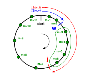
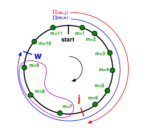
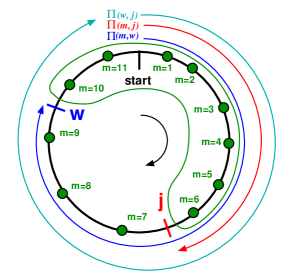
Figure 14: (Color) Two possible configurations with $s_{j}>s_{w}$ (left) and $s_{w}>s_{j}$ (center, wrong, and right, correct). See text for a detailed explanation.

By inserting Eqs. (226)-(226) into Eqs. (221)-(222) the explicit dependence of the ORM diagonal blocks upon the quadrupole error is derived, namely

$$\delta O^{(xx)}_{wj} \simeq -\sum\limits_{m=1}^{M}{\frac{\sqrt{\beta_{j,x}^{(mod)}\beta_{w,x}^{(mod)}}\beta_{m,x}^{(mod)}}{2\sin{(\pi Q_{x}^{(mod)})}}\Bigg{\{}\frac{\cos{(\Delta\phi_{x,wj}^{(mod)}-\pi Q_{x}^{(mod)})}}{4\sin{(2\pi Q_{x}^{(mod)})}}\Big{[}\cos{(2\Delta\phi_{x,mj}^{(mod)}-2\pi Q_{x})}+\cos{(2\Delta\phi_{x,mw}^{(mod)}-2\pi Q_{x})}\Big{]}}$$ (228)

$$\hskip 122.34692pt+\frac{\ \sin{(\Delta\phi_{x,wj}^{(mod)}-\pi Q_{x}^{(mod)})}}{4\sin{(2\pi Q_{x}^{(mod)})}}\Big{[}\sin{(2\Delta\phi_{x,mj}^{(mod)}-2\pi Q_{x})}-\ \sin{(2\Delta\phi_{x,mw}^{(mod)}-2\pi Q_{x})}\Big{]}$$

$$\hskip 91.04872pt+\frac{1}{2}\sin{(\Delta\phi_{x,wj}^{(mod)}-\pi Q_{x}^{(mod)})}\left[\Pi(m,j)-\Pi(m,w)+\Pi(j,w)\right]+\frac{\cos{(\Delta\phi_{x,wj}^{(mod)})}}{4\sin{(\pi Q_{x}^{(mod)})}}\Bigg{\}}\delta K_{m,1}\ ,$$

$$\delta O^{(yy)}_{wj} \simeq +\sum\limits_{m=1}^{M}{\frac{\sqrt{\beta_{j,y}^{(mod)}\beta_{w,y}^{(mod)}}\beta_{m,y}^{(mod)}}{2\sin{(\pi Q_{y}^{(mod)})}}\Bigg{\{}\frac{\cos{(\Delta\phi_{y,wj}^{(mod)}-\pi Q_{y}^{(mod)})}}{4\sin{(2\pi Q_{y}^{(mod)})}}\Big{[}\cos{(2\Delta\phi_{y,mj}^{(mod)}-2\pi Q_{y})}+\cos{(2\Delta\phi_{y,mw}^{(mod)}-2\pi Q_{y})}\Big{]}}$$

$$\hskip 122.34692pt+\frac{\ \sin{(\Delta\phi_{y,wj}^{(mod)}-\pi Q_{y}^{(mod)})}}{4\sin{(2\pi Q_{y}^{(mod)})}}\Big{[}\sin{(2\Delta\phi_{y,mj}^{(mod)}-2\pi Q_{y})}-\ \sin{(2\Delta\phi_{y,mw}^{(mod)}-2\pi Q_{y})}\Big{]}$$

$$\hskip 91.04872pt+\frac{1}{2}\sin{(\Delta\phi_{y,wj}^{(mod)}-\pi Q_{y}^{(mod)})}\left[\Pi(m,j)-\Pi(m,w)+\Pi(j,w)\right]+\frac{\cos{(\Delta\phi_{y,wj}^{(mod)})}}{4\sin{(\pi Q_{y}^{(mod)})}}\Bigg{\}}\delta K_{m,1}\ ,$$

where the remainder $O(\delta K_{1}^{2})$ has been omitted. From the above equations, analytic expressions for the betatronic part of the response matrix $\mathbf{N}$ of Eq. (16), i.e. of the derivative of $\delta O^{(xx)}_{wj}$ and $\delta O^{(yy)}_{wj}$ with respect to $\delta K_{m,1}$, are derived

$$N^{(xx)}_{wj,m} \simeq -\frac{\sqrt{\beta_{j,x}^{(mod)}\beta_{w,x}^{(mod)}}\beta_{m,x}^{(mod)}}{2\sin{(\pi Q_{x}^{(mod)})}}\Bigg{\{}\frac{\cos{(\Delta\phi_{x,wj}^{(mod)}-\pi Q_{x}^{(mod)})}}{4\sin{(2\pi Q_{x}^{(mod)})}}\Big{[}\cos{(2\Delta\phi_{x,mj}^{(mod)}-2\pi Q_{x})}+\cos{(2\Delta\phi_{x,mw}^{(mod)}-2\pi Q_{x})}\Big{]}$$ (229)

$$\hskip 102.43008pt+\frac{\ \sin{(\Delta\phi_{x,wj}^{(mod)}-\pi Q_{x}^{(mod)})}}{4\sin{(2\pi Q_{x}^{(mod)})}}\Big{[}\sin{(2\Delta\phi_{x,mj}^{(mod)}-2\pi Q_{x})}-\ \sin{(2\Delta\phi_{x,mw}^{(mod)}-2\pi Q_{x})}\Big{]}$$

$$\hskip 102.43008pt+\frac{1}{2}\sin{(\Delta\phi_{x,wj}^{(mod)}-\pi Q_{x}^{(mod)})}\left[\Pi(m,j)-\Pi(m,w)+\Pi(j,w)\right]+\frac{\cos{(\Delta\phi_{x,wj}^{(mod)})}}{4\sin{(\pi Q_{x}^{(mod)})}}\Bigg{\}}\ ,$$

$$N^{(yy)}_{wj,m} \simeq +\frac{\sqrt{\beta_{j,y}^{(mod)}\beta_{w,y}^{(mod)}}\beta_{m,y}^{(mod)}}{2\sin{(\pi Q_{y}^{(mod)})}}\Bigg{\{}\frac{\cos{(\Delta\phi_{y,wj}^{(mod)}-\pi Q_{y}^{(mod)})}}{4\sin{(2\pi Q_{y}^{(mod)})}}\Big{[}\cos{(2\Delta\phi_{y,mj}^{(mod)}-2\pi Q_{y})}+\cos{(2\Delta\phi_{y,mw}^{(mod)}-2\pi Q_{y})}\Big{]}$$

$$\hskip 102.43008pt+\frac{\ \sin{(\Delta\phi_{y,wj}^{(mod)}-\pi Q_{y}^{(mod)})}}{4\sin{(2\pi Q_{y}^{(mod)})}}\Big{[}\sin{(2\Delta\phi_{y,mj}^{(mod)}-2\pi Q_{y})}-\ \sin{(2\Delta\phi_{y,mw}^{(mod)}-2\pi Q_{y})}\Big{]}$$

$$\hskip 102.43008pt+\frac{1}{2}\sin{(\Delta\phi_{y,wj}^{(mod)}-\pi Q_{y}^{(mod)})}\left[\Pi(m,j)-\Pi(m,w)+\Pi(j,w)\right]+\frac{\cos{(\Delta\phi_{y,wj}^{(mod)})}}{4\sin{(\pi Q_{y}^{(mod)})}}\Bigg{\}}\ ,$$

where again the remainder, this time linear in $\delta K_{1}$, has been omitted. The function $\Pi(a,b)$ is defined in Eq. (227), whereas the (always positive) phase advance $\Delta\phi_{ab}$ is to be computed according to Eq. (155).

A.2 ORM response due to skew quadrupole fields

In this section explicit formulas for the evaluation of the impact of a skew quadrupole integrated strength $J_{1}$ on the off-diagonal blocks of the ORM, $O^{(xy)}_{wj}$ and $O^{(yx)}_{wj}$ of Eq. (214), are derived. These equations allow the direct computation of the matrix $\mathbf{S}$ of Eq. (22) from the C-S parameters with no need of computing numerically the derivative of the ORM with respect to $J_{1}$. It is assumed that the analysis of the ORM diagonal blocks is already carried out and a model comprising focusing errors is available, so to be able to compute the actual C-S parameters. These, and not the ideal ones, are to be used in the final formulas to ensure an RMS error within a few percents (numerical simulations showed that if the ideal C-S are used the discrepancy may increase up to $20\%$ for the old ESRF storage ring with the same beta-beating of Fig. 1). If large betatron coupling is present in the machine, the C-S parameters are affected by coupling RDTs, as shown in Ref. prstab_esr_coupling : This will corrupt the overall analysis and an iterative process of measurement and correction of linear lattice errors (focusing and coupling) is required.

From Eqs. (213), (214), the off-diagonal block corresponding to the horizontal orbit response to a vertical deflection reads

$$O^{(xy)}_{wj} = \sqrt{\beta_{j,x}\beta_{w,y}}\Re\left\{i(P_{14,wj}-P_{13,wj})\right\}\ ,$$

$$\simeq \sqrt{\beta_{j,x}\beta_{w,y}}\Re\left\{i\left[2if_{1010,w}\frac{e^{i\Delta\phi_{x,wj}}}{1-e^{i2\pi Q_{x}}}-2if_{1010,j}\frac{e^{-i\Delta\phi_{y,wj}}}{1-e^{-i2\pi Q_{y}}}-2if_{1001,w}\frac{e^{i\Delta\phi_{x,wj}}}{1-e^{i2\pi Q_{x}}}+2if_{1001,j}\frac{e^{i\Delta\phi_{y,wj}}}{1-e^{i2\pi Q_{y}}}\right]\right\}\ ,$$

where higher-order terms $\propto O(f^{2})$ have been neglected. By making use of the following identities and definitions

$$\frac{2i}{1-e^{\pm 2iz}}=\mp\frac{e^{\mp iz}}{\sin{z}}\qquad,\hskip 28.45274pt\tau_{z,ab}=\Delta\phi_{z,ab}-\pi Q_{z}\ ,\quad z=x,y\quad.$$ (231)

Eq. (A.2) simplifies to

$$O^{(xy)}_{wj} \simeq \sqrt{\beta_{j,x}\beta_{w,y}}\Re\left\{i\left[-f_{1010,w}\frac{e^{i\tau_{x,wj}}}{\sin{\pi Q_{x}}}-f_{1010,j}\frac{e^{-i\tau_{y,wj}}}{\sin{\pi Q_{y}}}+f_{1001,w}\frac{e^{i\tau_{x,wj}}}{\sin{\pi Q_{x}}}-f_{1001,j}\frac{e^{i\tau_{y,wj}}}{\sin{\pi Q_{y}}}\right]\right\}\ .$$ (232)

The coupling RDTs of Eq. (27) can be also written as

$$f_{{\tiny\begin{array}[]{c}1001\\ 1010\end{array}},\ j}\simeq\frac{\sum\limits_{m=1}^{M}J_{m,1}\sqrt{\beta_{m,x}\beta_{m,y}}e^{i(\Delta\phi_{x,mj}\mp\Delta\phi_{y,mj})}}{4(1-e^{2\pi i(Q_{u}\mp Q_{v})})}=\frac{i}{8\sin{[\pi(Q_{x}\mp Q_{y})]}}\sum\limits_{m=1}^{M}J_{m,1}{\sqrt{\beta_{m,x}\beta_{m,y}}e^{i(\tau_{x,mj}\mp\tau_{y,mj})}}\ ,\quad$$ (235)

where again higher order terms $\propto O(J_{1}^{2})$ are ignored. After replacing the RDTs in Eq. (232) with the above expression, the off-diagonal block can be eventually written as a function of the skew quadrupole strength $J_{m,1}$:

$$O^{(xy)}_{wj}\hskip-1.42271pt \simeq \hskip-4.26773pt\sum\limits_{m=1}^{M}\frac{J_{m,1}}{8}\sqrt{\beta_{j,x}\beta_{w,y}\beta_{m,x}\beta_{m,y}}\left\{\frac{1}{\sin{[\pi(Q_{x}-Q_{y})]}}\left[\frac{\cos{(\tau_{x,mj}-\tau_{y,mj}+\tau_{y,wj})}}{\sin{\pi Q_{y}}}-\frac{\cos{(\tau_{x,mw}-\tau_{y,mw}+\tau_{x,wj})}}{\sin{\pi Q_{x}}}\right]\right.$$

$$\hskip 119.50148pt\left.+\frac{1}{\sin{[\pi(Q_{x}+Q_{y})]}}\left[\frac{\cos{(\tau_{x,mj}+\tau_{y,mj}-\tau_{y,wj})}}{\sin{\pi Q_{y}}}+\frac{\cos{(\tau_{x,mw}+\tau_{y,mw}+\tau_{x,wj})}}{\sin{\pi Q_{x}}}\right]\right\}.$$

(236)

The same procedure applied to the vertical orbit response to a horizontal steerer results in

$$O^{(yx)}_{wj}\hskip-1.42271pt \simeq \hskip-4.26773pt\sum\limits_{m=1}^{M}\frac{J_{m,1}}{8}\sqrt{\beta_{j,y}\beta_{w,x}\beta_{m,x}\beta_{m,y}}\left\{\frac{1}{\sin{[\pi(Q_{x}-Q_{y})]}}\left[-\frac{\cos{(\tau_{x,mj}-\tau_{y,mj}-\tau_{x,wj})}}{\sin{\pi Q_{x}}}+\frac{\cos{(\tau_{x,mw}-\tau_{y,mw}-\tau_{y,wj})}}{\sin{\pi Q_{y}}}\right]\right.$$

$$\hskip 119.50148pt\left.+\frac{1}{\sin{[\pi(Q_{x}+Q_{y})]}}\left[\frac{\cos{(\tau_{x,mj}+\tau_{y,mj}-\tau_{x,wj})}}{\sin{\pi Q_{x}}}+\frac{\cos{(\tau_{x,mw}+\tau_{y,mw}+\tau_{y,wj})}}{\sin{\pi Q_{y}}}\right]\right\}.$$

(237)

From the above equations, analytic expressions for the betatronic part of the response matrix $\mathbf{S}$ of Eq. (22), i.e. of the derivative of $\delta O^{(xy)}_{wj}$ and $\delta O^{(yx)}_{wj}$ with respect to $J_{m,1}$, are derived

$$S^{(xy)}_{wj,m} \simeq \frac{1}{8}\sqrt{\beta_{j,x}\beta_{w,y}\beta_{m,x}\beta_{m,y}}\left\{\frac{1}{\sin{[\pi(Q_{x}-Q_{y})]}}\left[\frac{\cos{(\tau_{x,mj}-\tau_{y,mj}+\tau_{y,wj})}}{\sin{\pi Q_{y}}}-\frac{\cos{(\tau_{x,mw}-\tau_{y,mw}+\tau_{x,wj})}}{\sin{\pi Q_{x}}}\right]\right.$$ (238)

$$\hskip 92.47145pt\left.+\frac{1}{\sin{[\pi(Q_{x}+Q_{y})]}}\left[\frac{\cos{(\tau_{x,mj}+\tau_{y,mj}-\tau_{y,wj})}}{\sin{\pi Q_{y}}}+\frac{\cos{(\tau_{x,mw}+\tau_{y,mw}+\tau_{x,wj})}}{\sin{\pi Q_{x}}}\right]\right\}\ ,$$

$$S^{(yx)}_{wj,m} \simeq \frac{1}{8}\sqrt{\beta_{j,y}\beta_{w,x}\beta_{m,x}\beta_{m,y}}\left\{\frac{1}{\sin{[\pi(Q_{x}-Q_{y})]}}\left[-\frac{\cos{(\tau_{x,mj}-\tau_{y,mj}-\tau_{x,wj})}}{\sin{\pi Q_{x}}}+\frac{\cos{(\tau_{x,mw}-\tau_{y,mw}-\tau_{y,wj})}}{\sin{\pi Q_{y}}}\right]\right.$$

$$\hskip 92.47145pt\left.+\frac{1}{\sin{[\pi(Q_{x}+Q_{y})]}}\left[\frac{\cos{(\tau_{x,mj}+\tau_{y,mj}-\tau_{x,wj})}}{\sin{\pi Q_{x}}}+\frac{\cos{(\tau_{x,mw}+\tau_{y,mw}+\tau_{y,wj})}}{\sin{\pi Q_{y}}}\right]\right\}\ ,$$

where again the remainder, this time linear in $J_{1}$, has been omitted. $\tau_{ab}$ is defined in Eq. (231) from the phase advance $\Delta\phi_{ab}$ which is to be computed according to Eq. (155). The C-S parameters refer to the linear lattice including focusing errors.

A.3 Impact of sextupoles in the ORM measurement

Equations (228) and (237) have been derived ignoring the presence of sextupoles in the lattice. In reality, the orbit distortion at sextupoles induced by steerer magnets generates normal and skew quadrupole feed-down fields, $\delta K_{m,1}=-K_{m,2}x_{m,\rm c.o.}$ and $J_{m,1}=K_{m,2}y_{m,\rm c.o.}$, where $K_{m,2}$ denotes the integrated strength of the sextupole $m$ and $(x_{m,\rm c.o.},\ y_{m,\rm c.o.})$ is the corresponding closed orbit. Horizontal and vertical dipolar feed-down fields proportional to $(x_{m,\rm c.o.}^{2},\ y_{m,\rm c.o.}^{2})$ are also generated.

From Eqs. (II) and (35) the closed orbit at a generic BPM $j$ induced by a steerer kick $\theta_{w}$ can be written as

$$x_{j}=O_{wj}\theta_{w}\quad\Rightarrow\quad x_{j}=\left[O_{wj}^{(mod)}+\sum_{m}{N_{wj,m}\delta K_{m,1}}\right]\theta_{w}\ ,$$ (239)

where $O_{wj}^{(mod)}$ is the ORM element for the ideal lattice. The focusing errors would then stem from quadrupole imperfections and from the feed-down (quadrupolar and dipolar) generated by sextupoles, namely

$$x_{j}=\left[O_{wj}^{(mod)}+\sum_{m}{N_{wj,m}^{(Q)}\delta K_{m,1}}-\sum_{m}{N_{wj,m}^{(S)}(K_{m,2}x_{m,\rm c.o.})}+O(x_{m,\rm c.o.}^{2})\right]\theta_{w}\ .$$ (240)

The ORM is usually measured by recording the orbit distortion $x_{j,\pm}$ generated by two opposite steerer strengths $\pm\theta_{w}$, with $Q_{wj}=(x_{j,+}-x_{j,-})/(2\theta_{w})$. In the presence of sextupoles, the two orbits read

$$x_{j,+} = \left[O_{wj}^{(mod)}+\sum_{m}{N_{wj,m}^{(Q)}\delta K_{m,1}}-\sum_{m}{N_{wj,m}^{(S)}(K_{m,2}x_{m,\rm c.o.})}+O(x_{m,\rm c.o.}^{2})\right]\theta_{w}\ ,$$ (241)

$$x_{j,-} = -\left[O_{wj}^{(mod)}+\sum_{m}{N_{wj,m}^{(Q)}\delta K_{m,1}}+\sum_{m}{N_{wj,m}^{(S)}(K_{m,2}x_{m,\rm c.o.})}+O(x_{m,\rm c.o.}^{2})\right]\theta_{w}\ ,$$ (242)

where it is assumed that lattice errors are sufficiently small to have $x_{m,\rm c.o.,+}\simeq-x_{m,\rm c.o.,-}$. The measured ORM then is

$$Q_{wj}=O_{wj}^{(mod)}+\sum_{m}{N_{wj,m}^{(Q)}\delta K_{m,1}}+O(x_{m,\rm c.o.}^{2})\ .$$ (243)

Since $x_{m,\rm c.o.}\propto\theta_{w}$, the error is proportional to $\theta_{w}^{2}$. Equivalent considerations apply to the vertical orbit.

It is worthwhile noticing that the cancellation of the quadrupolar terms generated by sextupoles does not disappear if the orbit distortion is measured with an asymmetric perturbation, i.e. $\theta_{w,+}\neq-\theta_{w,-}$.

Appendix B Derivation of chromatic functions

In this appendix analytical formulas for the chromatic functions (linear and nonlinear dispersion, chromaticity, chromatic beating and chromatic coupling) are derived. In order to greatly simplify the mathematics, it is assumed that focusing errors $\delta K_{1}$ are included in the model and in the computation of the C-S parameters, as done for the evaluation of betatron coupling. This requires that the analysis of the diagonal blocks of the ORM be carried out before evaluating the chromatic functions.

Another assumption made here is that the edge focusing provided by nonzero dipole pole-face angles is negligible, the magnetic modelling being based on the multipolar expansion of Eq. (24). This may introduce a systematic error in the evaluation of the chromatic functions from the following analytic formulas. However, for the calibration of sextupole magnets and the correction of the chromatic functions, these formulas can still be effectively used, since any systematic error is canceled out.

The Hamiltonian in complex C-S coordinates of Eq. (159) is the starting point for the study of the 4D betatron motion. Chromatic effects may be inferred from the same Hamiltonian after replacing the betatron coordinates with the ones including dispersive terms:

$$\left\{\begin{aligned} x\rightarrow x+D_{x}\delta\\ p_{x}\rightarrow p_{x}+D_{x}^{\prime}\delta\end{aligned}\right.\hskip 5.69054pt\Rightarrow\hskip 5.69054pt\left\{\begin{aligned} \tilde{x}\rightarrow\tilde{x}+\tilde{D}_{x}\delta\\ \tilde{p}_{x}\rightarrow\tilde{p}_{x}+\tilde{D}_{x}^{\prime}\delta\end{aligned}\right.\hskip 14.22636pt,\hskip 14.22636pt\left\{\begin{aligned} y\rightarrow y+D_{y}\delta\\ p_{y}\rightarrow p_{y}+D_{y}^{\prime}\delta\end{aligned}\right.\hskip 5.69054pt\Rightarrow\hskip 5.69054pt\left\{\begin{aligned} \tilde{y}\rightarrow\tilde{y}+\tilde{D}_{y}\delta\\ \tilde{p}_{y}\rightarrow\tilde{p}_{y}+\tilde{D}_{y}^{\prime}\delta\end{aligned}\right.\quad,\qquad$$ (244)

where $\delta=(p-p_{0})/p_{0}$ represents the relative deviation from the reference momentum, $D$ and $D^{\prime}$ denote the dispersion and its derivative in Cartesian coordinates, whereas $\tilde{D}$ and $\tilde{D}^{\prime}$ are the equivalent in the C-S coordinates. The above relations result in

$$\left\{\begin{aligned} h_{x,\pm}\rightarrow h_{x,\pm}+d_{x,\pm}\delta\\ h_{y,\pm}\rightarrow h_{y,\pm}+d_{y,\pm}\delta\end{aligned}\right.\hskip 14.22636pt \hskip 14.22636pt\left\{\begin{aligned} d_{x,\pm}=\tilde{D}_{x}\pm i\tilde{D}_{x}^{\prime}\\ d_{y,\pm}=\tilde{D}_{y}\pm i\tilde{D}_{y}^{\prime}\end{aligned}\right.\ .\quad\qquad$$ , (245)

$d_{\pm}$ represents hence the dispersion in the complex C-S coordinates. The dependence on the particle energy is contained also in the Hamiltonian coefficients of Eq. (159) $h_{m,pqrt}$ through the magnetic rigidity and reads

$$\left\{\begin{aligned} K_{m,n-1}\rightarrow\frac{K_{m,n-1}}{1+\delta}\\ J_{m,n-1}\rightarrow\frac{J_{m,n-1}}{1+\delta}\end{aligned}\right.\hskip 14.22636pt\Rightarrow\hskip 14.22636pth_{m,pqrt}\rightarrow\displaystyle{\frac{h_{m,pqrt}}{1+\delta}}=h_{m,pqrt}(1-\delta+\delta^{2}+...\ )\ .\qquad$$ (246)

By substituting Eqs. (245)-(246) in Eq. (159) the energy-dependent Hamiltonian term (up to second order in $\delta$) reads

$$\tilde{H}_{m,pqrtd} \rightarrow h_{m,pqrtd}h_{m,x,+}^{p}h_{m,x,-}^{q}h_{m,y,+}^{r}h_{m,y,-}^{t}\delta^{d}$$

$$\rightarrow h_{m,lkno}(1-\delta+\delta^{2})(h_{m,x,+}+d_{m,x,+}\delta)^{l}(h_{m,x,-}+d_{m,x,-}\delta)^{k}(h_{m,y,+}+d_{m,y,+}\delta)^{n}(h_{m,y,-}+d_{m,y,-}\delta)^{o}\ \ .$$

Note that in the last row generic indices $lkno$ replace the initial ones $pqrt$ because several combinations of the former may contribute to generate the Hamiltonian term $\tilde{H}_{pqrtd}$ when going off momentum $d>0$. The binomials may indeed be expanded as

$$\tilde{H}_{m,pqrtd} \rightarrow h_{m,lkno}(1-\delta+\delta^{2})\sum_{a=0}^{l}{\left(\begin{array}[]{c}l\\ a\end{array}\right)}h_{m,x,+}^{l-a}(d_{m,x,+}\delta)^{a}\sum_{b=0}^{k}{\left(\begin{array}[]{c}k\\ b\end{array}\right)}h_{m,x,-}^{k-b}(d_{m,x,-}\delta)^{b}\times$$ (257)

$$\hskip 82.51299pt\sum_{c=0}^{n}{\left(\begin{array}[]{c}n\\ c\end{array}\right)}h_{m,y,+}^{n-c}(d_{m,y,+}\delta)^{c}\sum_{e=0}^{o}{\left(\begin{array}[]{c}o\\ e\end{array}\right)}h_{m,y,-}^{o-e}(d_{m,y,-}\delta)^{e}\qquad,$$

where $\left(\begin{array}[]{c}l\\ a\end{array}\right)=\displaystyle\frac{l!}{a!(l-a)!}$ is the binomial coefficient. Before deriving the chromatic observables (chromaticity, chromatic beta-beating, chromatic coupling and dispersion) from the Hamiltonian terms $\tilde{H}_{m,pqrtd}$, it is worthwhile to distinguish the different nature of the Hamiltonian terms of Eq. (257).

• $\mathbf{p+q+r+t=1,\ d=0}$, orbit-like terms: The magnetic elements corresponding to these terms define the orbit. Since the reference orbit is assumed to be known, only dipole errors $\delta K_{0}$ and $J_{0}$ (for planar rings $\delta J_{0}=J_{0}$) inducing orbit distortion shall be used in the definition of $\tilde{H}_{pqrtd}$.

  $$\left\{\begin{aligned} \displaystyle p+q+r+t=1\\ d=0\end{aligned}\right.\quad\Rightarrow\quad\delta K_{0},\ J_{0}\ \hbox{ in Eq.~{}\eqref{eq:h_Vs_KJ}}\ .$$ (258)

• $\mathbf{p+q+r+t=1,\ d=1}$, dispersion-like terms: The magnetic elements corresponding to these terms define the linear dependence of the orbit on $\delta$. This is generated by the linear dependence of the bending angles $K_{0}$ (including possible field errors $\delta K_{0}$) on the beam energy and on the linear optics. The latter depends on $\delta$ too, though to first order ($d=1$) this dependence is to be ignored (it may not be neglected when $d=2$). It is assumed that the linear optics is known through the C-S parameters and that focusing errors are included in the model, which is equivalent to say that with respect to the the used C-S parameters they are zero, $\delta K_{1}=0$. Betatron coupling may be instead non-zero, as well as vertical deflections $J_{0}$, if any.

  $$\left\{\begin{aligned} \displaystyle p+q+r+t=1\\ d=1\end{aligned}\right.\quad\Rightarrow\quad K_{0},\ J_{0},\ \delta K_{1}(=0),\ J_{1}\hbox{ in Eq.~{}\eqref{eq:h_Vs_KJ}}\ .$$ (259)

• $\mathbf{p+q+r+t=2,\ d=1}$, betatron-like terms: The magnetic elements corresponding to these terms define the linear dependence of the betatron motion on $\delta$. This is generated by the dependence of the normalized quadrupole strengths on the beam energy and on the additional focusing provided by the quadrupolar feed-down field experienced by the beam when entering the sextupoles off axis. There is no dependence on the dipolar fields, the betatron-like terms describing only the motion around the closed orbit.

  $$\left\{\begin{aligned} \displaystyle p+q+r+t=2\\ d=1\end{aligned}\right.\quad\Rightarrow\quad K_{1},\ J_{1},\ K_{2},\ J_{2}\ \hbox{in Eq.~{}\eqref{eq:h_Vs_KJ}}\ .$$ (260)

• $\mathbf{p+q+r+t=1,\ d=2}$, second-order dispersion-like terms: This higher-order dependence of the beam orbit on the energy imposes the inclusion of the dependence of the focusing lattice on $\delta$, i.e. quadrupole and sextupole strengths

  $$\left\{\begin{aligned} \displaystyle p+q+r+t=1\\ d=2\end{aligned}\right.\quad\Rightarrow\quad K_{0},\ J_{0},\ K_{1},\ J_{1}\ ,\ K_{2},\ J_{2}\ \hbox{in Eq.~{}\eqref{eq:h_Vs_KJ}}\ .$$ (261)

B.1 First-order chromatic terms (d=1)

Among all elements in the r.h.s. of Eq. (257) only those proportional to $\delta$ are kept, along with those proportional to $h_{m,x,+}^{p}h_{m,x,-}^{q}h_{m,y,+}^{r}h_{m,y,-}^{t}$. The Hamiltonian terms linear in $\delta$ read

$$\tilde{H}_{m,pqrt1} \rightarrow h_{m,lkno}(1-\delta)\sum_{a=0}^{l}\sum_{b=0}^{k}\sum_{c=0}^{n}\sum_{e=0}^{o}{\left(\hskip-2.84526pt\begin{array}[]{c}l\\ a\end{array}\hskip-2.84526pt\right)}{\left(\hskip-2.84526pt\begin{array}[]{c}k\\ b\end{array}\hskip-2.84526pt\right)}{\left(\hskip-2.84526pt\begin{array}[]{c}n\\ c\end{array}\hskip-2.84526pt\right)}{\left(\hskip-2.84526pt\begin{array}[]{c}o\\ e\end{array}\hskip-2.84526pt\right)}h_{m,x,+}^{l-a}h_{m,x,-}^{k-b}h_{m,y,+}^{n-c}h_{m,y,-}^{o-e}d_{m,x,+}^{\ a}d_{m,x,-}^{\ b}d_{m,y,+}^{\ c}d_{m,y,-}^{\ e}\times$$ (271)

$$\hskip 207.7052pt\delta^{a+b+c+e},$$

where all sets of indices $abce$ and $lkno$ satisfying the following systems are kept:

$$\left\{\begin{array}[]{l}l-a=p\\ k-b=q\\ n-c=r\\ o-e=t\\ a+b+c+e=1\end{array}\right.\qquad\hbox{and}\qquad\left\{\begin{array}[]{l}l-a=p\\ k-b=q\\ n-c=r\\ o-e=t\\ a+b+c+e=0\end{array}\right.\quad.$$ (282)

The two systems stem from the magnetic rigidity term $(1-\delta)$. After some algebra, the Hamiltonian terms linear in $\delta$ read

$$\tilde{H}_{m,pqrt1} \rightarrow h_{m,pqrt1}h_{m,x,+}^{p}h_{m,x,-}^{q}h_{m,y,+}^{r}h_{m,y,-}^{t}\delta$$ (283)

$$h_{m,pqrt1} = (p+1)h_{m,(p+1)qrt}d_{m,x,+}+(q+1)h_{m,p(q+1)rt}d_{m,x,-}+$$ (284)

$$(r+1)h_{m,pq(r+1)t}d_{m,y,+}+(t+1)h_{m,pqr(t+1)}d_{m,y,-}-h_{m,pqrt}\quad.$$

B.2 Linear dispersion

The on-momentum Hamiltonian of Eq. (177) needs to be extended to include a dependence on the energy deviation $\delta$. A second-order expansion reads

$$\tilde{H}_{m} = h_{m,1000}h_{m,x,+}+h_{m,0100}h_{m,x,-}+h_{m,0010}h_{m,y,+}+h_{m,0001}h_{m,y,-}+$$ (285)

$$(h_{m,10001}h_{m,x,+}+h_{m,01001}h_{m,x,-}+h_{m,00101}h_{m,y,+}+h_{m,00011}h_{m,y,-})\delta+$$

$$(h_{m,10002}h_{m,x,+}+h_{m,01002}h_{m,x,-}+h_{m,00102}h_{m,y,+}+h_{m,00012}h_{m,y,-})\delta^{2}+O(\delta^{3})\ .$$

Hereafter, the subscript $m$ corresponding to a generic magnet replaces here the label $w$ of a generic orbit corrector in Eq. (177), since we are no longer interested in the evaluation of an ORM, but rather of chromatic functions dependent on the strengths of magnets of different order (dipole, quadrupole and sextupole). The off-momentum generalization of Eq. (191) then reads

$$\delta\vec{h}_{m}=\left(\begin{array}[]{c}\delta h_{m,x,-}\\ \delta h_{m,x,+}\\ \delta h_{m,y,-}\\ \delta h_{m,y,+}\end{array}\right)=2i\left(\begin{array}[]{r}h_{m,1000}\\ -h_{m,0100}\\ h_{m,0010}\\ -h_{m,0001}\end{array}\right)\ +2i\left(\begin{array}[]{r}h_{m,10001}\\ -h_{m,01001}\\ h_{m,00101}\\ -h_{m,00011}\end{array}\right)\delta\ +2i\left(\begin{array}[]{r}h_{m,10002}\\ -h_{m,01002}\\ h_{m,00102}\\ -h_{m,00012}\end{array}\right)\delta^{2}\ \ +O(\delta^{3}).$$ (302)

The first terms in the r.h.s. are responsible for the orbit distortion, the second terms proportional to $\delta$ modify the linear dispersion $D$, whereas the last elements account for the derivative of the dispersion with respect to $\delta$, $D^{\prime}$. For the evaluation of linear dispersion, the Hamiltonian terms in the second vector of the r.h.s. of Eq. (302) are to be computed. These are evaluated from Eq. (284) ($d=1$), yielding

$$\left\{\begin{aligned} \displaystyle h_{m,10001}&=2h_{m,2000\ }d_{m,x,+}+h_{m,1100\ }d_{m,x,-}+h_{m,1010\ }d_{m,y,+}+h_{m,1001\ }d_{m,y,-}-h_{m,1000}\\ h_{m,01001}&=h_{m,1100\ }d_{m,x,+}+2h_{m,2000\ }d_{m,x,-}+h_{m,0110\ }d_{m,y,+}+h_{m,0101\ }d_{m,y,-}-h_{m,0100}\\ h_{m,00101}&=h_{m,1010\ }d_{m,x,+}+h_{m,0110\ }d_{m,x,-}+2h_{m,0020\ }d_{m,y,+}+h_{m,0011\ }d_{m,y,-}-h_{m,0010}\\ h_{m,00011}&=h_{m,1001\ }d_{m,x,+}+h_{m,0101\ }d_{m,x,-}+h_{m,0011\ }d_{m,y,+}+2h_{m,0002\ }d_{m,y,-}-h_{m,0001}\end{aligned}\right.\ .$$ (303)

The Hamiltonian coefficients $h_{m,pqrt}$ are computed from Eq. (A):

$$\left\{\begin{aligned} \displaystyle 2h_{m,2000}&=h_{m,1100}=-\frac{1}{4}\delta K_{m,1}\beta_{m,x}=0\\ 2h_{m,0020}&=h_{m,0011}=+\frac{1}{4}\delta K_{m,1}\beta_{m,y}=0\\ h_{m,1010}&=h_{m,1001}=h_{m,0110}=+\frac{1}{4}J_{m,1}\sqrt{\beta_{m,x}\beta_{m,y}}\\ h_{m,1000}&=h_{m,0100}=-\frac{1}{2}K_{m,0}\sqrt{\beta_{m,x}}\\ h_{m,0010}&=h_{m,0001}=+\frac{1}{2}J_{m,0}\sqrt{\beta_{m,y}}\end{aligned}\right.\ .$$ (304)

Since Hamiltonian terms with $p+q+r+t=1$ and $d=1$ are evaluated in Eq. (303), Eq. (259) applies and the main bending magnet horizontal angles $K_{0}$ (and vertical $J_{0}$, if any) are used, whereas the focusing errors are assumed to be included in the computation of the beta functions, hence $\delta K_{1}=0$. Equation (303) then reads

$$\left\{\begin{aligned} \displaystyle h_{m,10001}&=h_{m,1010\ }2\Re\left\{d_{m,y,\pm}\right\}-h_{m,1000}=+\frac{1}{2}\left(K_{m,0}+J_{m,1}D_{m,y}\right)\sqrt{\beta_{m,x}}\\ h_{m,01001}&=h_{m,10001}\\ h_{m,00101}&=h_{m,1010\ }2\Re\left\{d_{m,x,\pm}\right\}-h_{m,0010}=-\frac{1}{2}\left(J_{m,0}-J_{m,1}D_{m,x}\right)\sqrt{\beta_{m,y}}\\ h_{m,00011}&=h_{m,00101}\end{aligned}\right.\ ,$$ (305)

since $\Re\left\{d_{m,q,\pm}\right\}=D_{m,q}/\sqrt{\beta_{m,q}}$. Thus, the off-momentum closed orbit of Eq. (176) becomes

$$\vec{h}(j) = \mathbf{B}_{j}^{-1}\sum_{m=1}^{M}\left\{\frac{e^{i\mathbf{\Delta\phi}_{mj}}}{1-e^{i\mathbf{Q}}}\mathbf{B}_{m}\ i\left(\begin{array}[]{r}\left(K_{m,0}+J_{m,1}D_{m,y}\right)\sqrt{\beta_{m,x}}\\ -\left(K_{m,0}+J_{m,1}D_{m,y}\right)\sqrt{\beta_{m,x}}\\ -\left(J_{m,0}-J_{m,1}D_{m,x}\right)\sqrt{\beta_{m,y}}\\ \left(J_{m,0}-J_{m,1}D_{m,x}\right)\sqrt{\beta_{m,y}}\end{array}\right)\right\}\delta\quad.$$ (310)

The above expression simplifies greatly, since for the linear dispersion the effects of the normal form transformations $\mathbf{B}_{j}^{-1}$ and $\mathbf{B}_{m}$ are of higher order and shall be ignored here, hence leaving

$$\vec{h}(j) \simeq \sum_{m=1}^{M}\left\{\frac{e^{i\mathbf{\Delta\phi}_{mj}}}{1-e^{i\mathbf{Q}}}\ i\left(\begin{array}[]{r}\left(K_{m,0}+J_{m,1}D_{m,y}\right)\sqrt{\beta_{m,x}}\\ -\left(K_{m,0}+J_{m,1}D_{m,y}\right)\sqrt{\beta_{m,x}}\\ -\left(J_{m,0}-J_{m,1}D_{m,x}\right)\sqrt{\beta_{m,y}}\\ \left(J_{m,0}-J_{m,1}D_{m,x}\right)\sqrt{\beta_{m,y}}\end{array}\right)\right\}\delta\quad,$$ (315)

where now all C-S parameters and dispersion refer to the ideal lattice with no focusing errors and betatron coupling, though with possible vertical dispersion induced by vertical dipole terms. The complex dispersion vector $\vec{d}=(\tilde{d}_{x,-},\tilde{d}_{x,+},\tilde{d}_{y,-},\tilde{d}_{y,+})^{T}$ hence reads

$$\vec{d}(j) = \frac{\partial\vec{h}(j)}{\partial\delta}\simeq\sum_{m=1}^{M}\left\{\frac{e^{i\mathbf{\Delta\phi}_{mj}}}{1-e^{i\mathbf{Q}}}\ i\left(\begin{array}[]{r}\left(K_{m,0}+J_{m,1}D_{m,y}\right)\sqrt{\beta_{m,x}}\\ -\left(K_{m,0}+J_{m,1}D_{m,y}\right)\sqrt{\beta_{m,x}}\\ -\left(J_{m,0}-J_{m,1}D_{m,x}\right)\sqrt{\beta_{m,y}}\\ \left(J_{m,0}-J_{m,1}D_{m,x}\right)\sqrt{\beta_{m,y}}\end{array}\right)\right\}\ ,$$ (320)

from which both the horizontal and the vertical dispersion at a location $j$ can be inferred, since $D_{x}=\Re\left\{\tilde{d}_{x,-}\right\}\sqrt{\beta_{x}}$ and $D_{y}=\Re\left\{\tilde{d}_{y,-}\right\}\sqrt{\beta_{y}}$:

$$\vec{d}(j) \simeq i\sum_{m=1}^{M}\left\{\left(\begin{array}[]{c c c c}\frac{e^{i\Delta\phi_{x,mj}}}{1-e^{i2\pi Q_{x}}}&0&0&0\\ 0&\frac{e^{-i\Delta\phi_{x,mj}}}{1-e^{-i2\pi Q_{x}}}&0&0\\ 0&0&\frac{e^{i\Delta\phi_{y,mj}}}{1-e^{i2\pi Q_{y}}}&0\\ 0&0&0&\frac{e^{-i\Delta\phi_{y,mj}}}{1-e^{-i2\pi Q_{y}}}\end{array}\right)\left(\begin{array}[]{r}\left(K_{m,0}+J_{m,1}D_{m,y}\right)\sqrt{\beta_{m,x}}\\ -\left(K_{m,0}+J_{m,1}D_{m,y}\right)\sqrt{\beta_{m,x}}\\ -\left(J_{m,0}-J_{m,1}D_{m,x}\right)\sqrt{\beta_{m,y}}\\ \left(J_{m,0}-J_{m,1}D_{m,x}\right)\sqrt{\beta_{m,y}}\end{array}\right)\right\}\ ,$$ (329)

resulting in

$$\left\{\begin{aligned} D_{x}(j)&\simeq+\frac{\sqrt{\beta_{j,x}}}{2\sin{(\pi Q_{x})}}\sum_{m=1}^{M}\left(K_{m,0}+J_{m,1}D_{m,y}\right)\sqrt{\beta_{m,x}}\cos(\Delta\phi_{x,mj}-\pi Q_{x})\\ D_{y}(j)&\simeq-\frac{\sqrt{\beta_{j,y}}}{2\sin{(\pi Q_{y})}}\sum_{m=1}^{M}\left(J_{m,0}-J_{m,1}D_{m,x}\right)\sqrt{\beta_{m,y}}\cos(\Delta\phi_{y,mj}-\pi Q_{y})\end{aligned}\right.\ .$$ (330)

For consistency with the nomenclature used throughout this paper, the phase advance $\Delta\phi_{mj}$ is to be computed as in Eq. (155). If the mere difference between the two betatron phases at the positions $m$ and $j$ is used, the absolute value $|2\Delta\phi_{x,mj}|$ shall then be used, as done in textbooks, whose formulas for the ideal case are retrieved from Eq. (330) after removing betatron coupling ($J_{1}=0$) and vertical dispersion ($J_{0}=0$, $D_{m,y}=0$). Note that the above equations are still valid in the presence of focusing errors and betatron coupling, provided that the corresponding C-S parameters $\beta$ and $\phi$ and dispersion are used. $D_{m,y}$ in the r.h.s. of Eq. (330) shall then be the one generated by the vertical dipole fields $J_{0}$ (if any) but not by betatron coupling. Indeed, it is Eq. (330) that describes the entanglement between the horizontal and vertical dispersion functions due to skew quadrupole fields.

B.3 linear chromaticity

As second example of application of Eq. (284) the linear detuning Hamiltonian terms proportional to $\delta$ are evaluated. They are linked to the linear chromaticity. As shown in Ref. Andrea-arxiv , the Hamiltonian term at a generic position $j$ generated by all $M$ magnets reads

$$\tilde{H}_{pqrt}(j)=\sum_{m=1}^{M}\tilde{H}_{m}(j)=\sum_{m=1}^{M}{h_{m,pqrt}e^{i[(p-q)\Delta\phi_{x,mj}+(r-t)\Delta\phi_{y,mj}]}h_{m,x,+}^{p}h_{m,x,-}^{q}h_{m,y,+}^{r}h_{m,y,-}^{t}}\quad.$$ (331)

Without loss of generality we can expand the Hamiltonian terms at a location $j$ in a power series of $\delta$

$$\tilde{H}_{pqrt}(j,\delta)=\sum_{d\geq 0}\tilde{H}_{pqrtd}(j)\delta^{d}=\tilde{H}_{pqrt}(j)+\tilde{H}_{pqrt1}\delta+\tilde{H}_{pqrt2}(j)\delta^{2}+O(\delta^{3})\ ,$$ (332)

where $\tilde{H}_{pqrt}(j)$ is the geometric Hamiltonian of Eq. (331), whereas $\tilde{H}_{pqrt1}(j)$ is the corresponding first chromatic Hamiltonian,

$$\tilde{H}_{pqrt1}(j)=\sum_{m=1}^{M}{h_{m,pqrt1}e^{i[(p-q)\Delta\phi_{x,mj}+(r-t)\Delta\phi_{y,mj}]}h_{m,x,+}^{p}h_{m,x,-}^{q}h_{m,y,+}^{r}h_{m,y,-}^{t}}\delta\ ,$$ (333)

whose coefficients $h_{m,pqrt1}$ are those of Eq. (284).

Detuning terms are those with $p=q$ and $r=t$, hence independent of the betatron phases, since in the above expression the phases are all equal to 1 and the product of all coordinates is invariant, $h_{m,x,+}^{p}h_{m,x,-}^{p}h_{m,y,+}^{r}h_{m,y,-}^{r}=(2I_{x})^{p}(2I_{y})^{r}$. The first chromatic non-zero detuning coefficients are $h_{m,11001}$ and $h_{m,00111}$ in the horizontal and vertical planes, respectively. The substitution of those indices in Eq. (284) yields

$$\left\{\begin{array}[]{l}h_{m,11001}=2h_{m,2100}\ d_{m,x,+}+2h_{m,1200}\ d_{m,x,-}+\ h_{m,1110}\ d_{m,y,+}+\ h_{m,1101}\ d_{m,y,-}-h_{m,1100}\\ h_{m,00111}=\ h_{m,1011}\ d_{m,x,+}+\ h_{m,0111}\ d_{m,x,-}+2h_{m,0021}\ d_{m,y,+}+2h_{m,0012}\ d_{m,y,-}-h_{m,0011}\end{array}\right.\quad.$$ (336)

The Hamiltonian coefficients in the above r.h.s. may be made explicit via Eq. (A):

$$h_{m,2100} = h_{m,1200}=-\frac{1}{16}K_{m,2}\beta_{m,x}^{3/2}\quad,\quad h_{m,1110}=h_{m,1101}=+\frac{1}{8}J_{m,2}\beta_{m,x}\sqrt{\beta_{m,y}}\quad,\quad h_{m,1100}=-\frac{1}{4}K_{m,1}\beta_{m,x}\quad,\quad\qquad$$ (337)

$$h_{m,0021} = h_{m,0012}=-\frac{1}{16}J_{m,2}\beta_{m,y}^{3/2}\quad,\quad h_{m,1011}=h_{m,0111}=+\frac{1}{8}K_{m,2}\sqrt{\beta_{m,x}}\beta_{m,y}\quad,\quad h_{m,0011}=+\frac{1}{4}K_{m,1}\beta_{m,y}\quad.\quad\qquad$$ (338)

Eq. (336) then reads

$$\left\{\begin{array}[]{l}h_{m,11001}=4h_{m,2100}\Re\left\{d_{m,x,+}\right\}+2h_{m,1110}\Re\left\{d_{m,y,+}\right\}-h_{m,1100}\\ h_{m,00111}=2h_{m,1011}\Re\left\{d_{m,x,+}\right\}+4h_{m,0021}\Re\left\{d_{m,y,+}\right\}-h_{m,0011}\end{array}\right.\quad.$$ (341)

Since $\Re\left\{d_{m,q,+}\right\}=D_{m,q}/\sqrt{\beta_{m,q}}$, the two Hamiltonian coefficients become

$$\left\{\begin{array}[]{l}h_{m,11001}=+\displaystyle\frac{1}{4}\left(K_{m,1}-K_{m,2}D_{m,x}+J_{m,2}D_{m,y}\right)\beta_{m,x}\vspace{ 1.5mm}\\ h_{m,00111}=-\displaystyle\frac{1}{4}\left(K_{m,1}-K_{m,2}D_{m,x}+J_{m,2}D_{m,y}\right)\beta_{m,y}\end{array}\right.\quad.$$ (344)

As expected, both quantities are real and differ only by the sign and the beta functions, the argument within the parenthesis being the same in both planes. These indeed represent the effective quadrupole forces experienced by off-energy particles. The Hamiltonian accounting for all magnets is derived from Eq. (333),

$$\left\{\begin{array}[]{l}\tilde{H}_{11001}=+\displaystyle\frac{1}{4}\sum\limits_{m=1}^{M}\left(K_{m,1}-K_{m,2}D_{m,x}+J_{m,2}D_{m,y}\right)\beta_{m,x}\ h_{m,x,+}h_{m,x,-}\delta\vspace{ 1.5mm}\\ \tilde{H}_{00111}=-\displaystyle\frac{1}{4}\sum\limits_{m=1}^{M}\left(K_{m,1}-K_{m,2}D_{m,x}+J_{m,2}D_{m,y}\right)\beta_{m,y}\ h_{m,y,+}h_{m,y,-}\delta\end{array}\right.\quad,$$ (347)

or equivalently

$$\left\{\begin{array}[]{l}\displaystyle\tilde{H}_{11001}=h_{11001}(2J_{x})\delta=\sum\limits_{m=1}^{M}h_{m,11001}(2J_{x})\delta\\ \displaystyle\tilde{H}_{00111}=h_{00111}(2J_{y})\delta=\sum\limits_{m=1}^{M}h_{m,00111}(2J_{y})\delta\end{array}\right.\quad.$$ (350)

As expected, neither term depends on the betatron phases and hence on the longitudinal position $j$. The linear chromaticity is defined as

$$\left\{\begin{array}[]{l}\displaystyle Q_{x}^{\prime}=\frac{\partial Q_{x}}{\partial\delta}\bigg{|}_{\delta=0}\hskip-5.69054pt=\frac{\partial}{\partial\delta}\left(-{\frac{1}{2\pi}}\frac{\partial\left(\tilde{H}_{11000}+\tilde{H}_{11001}\delta\right)}{\partial J_{x}}\right)_{\delta=0}\hskip-5.69054pt=-\frac{h_{11001}}{\pi}=-\displaystyle\frac{1}{4\pi}\sum\limits_{m=1}^{M}\left(K_{m,1}-K_{m,2}D_{m,x}+J_{m,2}D_{m,y}\right)\beta_{m,x}\vspace{ 1.5mm}\\ \displaystyle Q_{y}^{\prime}=\frac{\partial Q_{y}}{\partial\delta}\bigg{|}_{\delta=0}\hskip-5.69054pt=\frac{\partial}{\partial\delta}\left(-{\frac{1}{2\pi}}\frac{\partial\left(\tilde{H}_{00110}+\tilde{H}_{00111}\delta\right)}{\partial J_{y}}\right)_{\delta=0}\hskip-5.69054pt=-\frac{h_{00111}}{\pi}=+\displaystyle\frac{1}{4\pi}\sum\limits_{m=1}^{M}\left(K_{m,1}-K_{m,2}D_{m,x}+J_{m,2}D_{m,y}\right)\beta_{m,y}\end{array}\right.\ .$$

(352)

$\tilde{H}_{11000}$ and $\tilde{H}_{00110}$ are both zero because focusing errors $\delta K_{1}$ are either zero or included in the model to compute the C-S parameters. The above relations require some comments. First, textbook formulas are retrieved when removing either vertical dispersion or the skew sextupole strengths $J_{2}$. Second, skew quadrupole fields $J_{1}$ do not influence explicitly linear chromaticity, at least to first order in the Hamiltonian truncation, of which more in Sec. B.8. Betatron coupling enters indirectly in Eq. (352) through vertical dispersion $D_{y}$.

B.4 Chromatic beating

Off-energy particles experience a non-zero closed orbit described by the dispersion function. When crossing normal sextupoles off axis, those particles are subjected to quadrupolar feed-down fields. This additional focusing results in modulated beta functions. Even an ideal lattice with no focusing error (i.e. no on-momentum geometric beta-beating) is unavoidably subjected to this chromatic modulation of the beta functions and hence to the corresponding half-integer resonance. The geometric beta-beating is described by the two RDTs $f_{2000}$ and $f_{0020}$. These in turn are generated by the geometric Hamiltonian coefficients $h_{2000}$ and $h_{0020}$, see Eq. (158). It is then natural to seek the source of chromatic beating in the two chromatic Hamiltonian coefficients $h_{20001}$ and $h_{00201}$ and to derive expressions for the linear dependence of the beta functions on $\delta$, i.e. $\partial\beta/\partial\delta$. From Eq. (284) we obtain

$$\left\{\begin{array}[]{l}h_{m,20001}=3h_{m,3000}\ d_{m,x,+}+\ h_{m,2100}\ d_{m,x,-}+\ h_{m,2010}\ d_{m,y,+}+\ h_{m,2001}\ d_{m,y,-}-h_{m,2000}\\ h_{m,00201}=\ h_{m,1020}\ d_{m,x,+}+\ h_{m,0120}\ d_{m,x,-}+3h_{m,0030}\ d_{m,y,+}+\ h_{m,0021}\ d_{m,y,-}-h_{m,0020}\end{array}\right.\quad.$$ (355)

Since in both cases $p+q+r+t=2$ and $d=1$, Eq. (260) applies and all Hamiltonian coefficients are to be computed from Eq. (A) using the total focusing strengths $K_{1}$ (nominal plus errors) as well as the sextupole strengths (normal and skew):

$$h_{m,2100} = 3h_{m,3000}=-\frac{1}{16}K_{m,2}\beta_{m,x}^{3/2}\ ,\quad h_{m,2010}=h_{m,2001}=+\frac{1}{16}J_{m,2}\beta_{m,x}\sqrt{\beta_{m,y}}\ ,\quad h_{m,2000}=-\frac{1}{8}K_{m,1}\beta_{m,x}\ ,\ \qquad$$ (356)

$$h_{m,0021} = 3h_{m,0030}=-\frac{1}{16}J_{m,2}\beta_{m,y}^{3/2}\ ,\quad h_{m,1020}=h_{m,0120}=+\frac{1}{16}K_{m,2}\sqrt{\beta_{m,x}}\beta_{m,y}\ ,\quad h_{m,0020}=+\frac{1}{8}K_{m,1}\beta_{m,y}\ .\ \qquad$$ (357)

Eq. (355) then reads

$$\left\{\begin{array}[]{l}h_{m,20001}=6h_{m,3000}\Re\left\{d_{m,x,+}\right\}+2h_{m,2010}\Re\left\{d_{m,y,+}\right\}-h_{m,2000}\\ h_{m,00201}=2h_{m,1020}\Re\left\{d_{m,x,+}\right\}+6h_{m,0030}\Re\left\{d_{m,y,+}\right\}-h_{m,0020}\end{array}\right.\quad.$$ (360)

Since $\Re\left\{d_{m,q,+}\right\}=D_{m,q}/\sqrt{\beta_{m,q}}$, the two Hamiltonian coefficients become

$$\left\{\begin{array}[]{l}h_{m,20001}=+\displaystyle\frac{1}{8}\left(K_{m,1}-K_{m,2}D_{m,x}+J_{m,2}D_{m,y}\right)\beta_{m,x}\vspace{ 1.5mm}\\ h_{m,00201}=-\displaystyle\frac{1}{8}\left(K_{m,1}-K_{m,2}D_{m,x}+J_{m,2}D_{m,y}\right)\beta_{m,y}\end{array}\right.\quad.$$ (363)

Note how the arguments in the above parenthesis are the same and equal to those of Eq. (344), this being the effective quadrupole strength experienced by off-energy particles. The Hamiltonian at a generic location $j$ accounting for all magnets is derived from Eq. (333) and reads

$$\left\{\begin{array}[]{l}\tilde{H}_{20001}(j)=\sum\limits_{m=1}^{M}h_{m,20001}\ h_{m,x,+}^{2}\delta=+\displaystyle\frac{1}{8}\sum\limits_{m=1}^{M}\left(K_{m,1}-K_{m,2}D_{m,x}+J_{m,2}D_{m,y}\right)\beta_{m,x}e^{2i\Delta\phi_{x,mj}}\ h_{m,x,+}^{2}\delta\vspace{ 1.5mm}\\ \tilde{H}_{00201}(j)=\sum\limits_{m=1}^{M}h_{m,00201}\ h_{m,y,+}^{2}\delta=-\displaystyle\frac{1}{8}\sum\limits_{m=1}^{M}\left(K_{m,1}-K_{m,2}D_{m,x}+J_{m,2}D_{m,y}\right)\beta_{m,y}e^{2i\Delta\phi_{y,mj}}\ h_{m,y,+}^{2}\delta\end{array}\right..$$ (366)

Conversely to the invariant detuning terms of Eq. (347), the chromatic beating terms are modulated at twice the betatron phase, as the geometric beta-beating. According to Eq. (158), the on-momentum beta-beating RDTs ($d=0$) read

$$f_{2000}(j)=\frac{\sum\limits_{m=1}^{M}h_{m,2000}e^{2i\Delta\phi_{x,mj}}}{1-e^{4\pi iQ_{x}}}\qquad,\qquad f_{0020}(j)=\frac{\sum\limits_{m=1}^{M}h_{m,0020}e^{2i\Delta\phi_{y,mj}}}{1-e^{4\pi iQ_{y}}}\quad,$$ (367)

which are both zero, since focusing errors $\delta K_{1}$ are assumed to be included in the model and hence $h_{m,2000}=h_{m,0020}=0$. The extension of the above relations to the off-momentum dynamics reads

$$\left\{\begin{array}[]{l}f_{2000}(j,\delta)=f_{2000}(j)+f_{20001}(j)\delta=\displaystyle\frac{\sum\limits_{m=1}^{M}h_{m,20001}e^{2i\Delta\phi_{x,mj}}}{1-e^{4\pi iQ_{x}}}\delta\quad,\qquad f_{20001}(j)=\displaystyle\frac{\partial f_{2000}(j,\delta)}{\partial\delta}\bigg{|}_{\delta=0}\\ \\ \displaystyle f_{0020}(j,\delta)=f_{0020}(j)+f_{00201}(j)\delta=\frac{\sum\limits_{m=1}^{M}h_{m,00201}e^{2i\Delta\phi_{y,mj}}}{1-e^{4\pi iQ_{y}}}\delta\quad,\qquad f_{00201}(j)=\displaystyle\frac{\partial f_{0020}(j,\delta)}{\partial\delta}\bigg{|}_{\delta=0}\end{array}\right.\quad.$$ (368)

The derivative of the two RDTs with respect to $\delta$ can then be written as

$$\left\{\begin{array}[]{l}f_{20001}(j)=\displaystyle\hskip-8.53581pt=\frac{\sum\limits_{m=1}^{M}h_{m,20001}e^{2i\Delta\phi_{x,mj}}}{1-e^{4\pi iQ_{x}}}=\frac{1}{8\left(1-e^{4\pi iQ_{x}}\right)}\sum\limits_{m=1}^{M}\left(K_{m,1}-K_{m,2}D_{m,x}+J_{m,2}D_{m,y}\right)\beta_{m,x}e^{2i\Delta\phi_{x,mj}}\\ \\ \displaystyle f_{00201}(j)=\displaystyle\hskip-8.53581pt=\frac{\sum\limits_{m=1}^{M}h_{m,00201}e^{2i\Delta\phi_{y,mj}}}{1-e^{4\pi iQ_{y}}}=\frac{-1}{8\left(1-e^{4\pi iQ_{y}}\right)}\sum\limits_{m=1}^{M}\left(K_{m,1}-K_{m,2}D_{m,x}+J_{m,2}D_{m,y}\right)\beta_{m,y}e^{2i\Delta\phi_{y,mj}}\end{array}\right.\ .$$ (369)

The dependence of the betatron tune on $\delta$, i.e. the linear chromaticity, is neglected since both $f_{20001}$ and $f_{00201}$ are multiplied by $\delta$ in Eq. (368). The on-momentum beta-beating reads Andrea-arxiv ; Andrea-Linear-arxiv

$$\left\{\begin{array}[]{l}\displaystyle\frac{\Delta\beta_{x}}{\beta_{x}}=2\sinh{(4|f_{2000}|)}\Big{[}\sinh{(4|f_{2000}|)}+\cosh{(4|f_{2000}|)}\sin{q_{2000}}\Big{]}\simeq 8|f_{2000}|\sin{q_{2000}}+O(|f_{2000}|^{2})\\ \\ \displaystyle\frac{\Delta\beta_{y}}{\beta_{y}}=2\sinh{(4|f_{0020}|)}\Big{[}\sinh{(4|f_{0020}|)}+\cosh{(4|f_{0020}|)}\sin{q_{0020}}\Big{]}\simeq 8|f_{0020}|\sin{q_{0020}}+O(|f_{0020}|^{2})\end{array}\right.\quad,$$ (373)

where $q_{2000}$ and $q_{0020}$ represent the phase of the two RDTs, $f=|f|e^{iq}$, and a first-order truncation has been performed, valid as long as $|f_{2000}|,\ |f_{0020}|\ll 1$, i.e. for weak beating. By noting that $|f|\sin{q}=\Im\left\{f\right\}$, the above formulas may be rewritten at a generic location $j$ as

$$\left\{\begin{array}[]{l}\displaystyle\beta_{x}(j)\simeq\beta_{x}^{(mod)}(j)+8\beta_{x}^{(mod)}(j)\Im\left\{f_{2000}(j)\right\}\\ \\ \displaystyle\beta_{y}(j)\simeq\beta_{y}^{(mod)}(j)+8\beta_{y}^{(mod)}(j)\Im\left\{f_{0020}(j)\right\}\end{array}\right.\quad.$$ (377)

Off-momentum particles will then experience the following beta functions

$$\left\{\begin{array}[]{l}\displaystyle\beta_{x}(j,\delta)\simeq\beta_{x}^{(mod)}(j)+8\beta_{x}^{(mod)}(j)\Im\left\{f_{2000}(j,\delta)\right\}\\ \\ \displaystyle\beta_{y}(j,\delta)\simeq\beta_{y}^{(mod)}(j)+8\beta_{y}^{(mod)}(j)\Im\left\{f_{0020}(j,\delta)\right\}\end{array}\right.\quad.$$ (381)

By making use of Eq. (368) with $f_{2000}=f_{0020}=0$, the above expressions truncated to first order in $\delta$ read

$$\left\{\begin{array}[]{l}\displaystyle\beta_{x}(j,\delta)\simeq\beta_{x}^{(mod)}(j)+8\beta_{x}^{(mod)}(j)\Im\left\{f_{20001}(j)\right\}\delta+O(\delta^{2})\\ \\ \displaystyle\beta_{y}(j,\delta)\simeq\beta_{y}^{(mod)}(j)+8\beta_{y}^{(mod)}(j)\Im\left\{f_{00201}(j)\right\}\delta+O(\delta^{2})\end{array}\right.\quad,$$ (385)

When going off momentum, the beta function is not the only quantity to change the linear phase space orbit and geometry, whose maximum normalized amplitude in the horizontal plane is given by $|\tilde{x}(j)_{\rm max}|=\sqrt{2J_{x}}$. Indeed, the invariant too is deformed by the change of energy, since $\sqrt{2J_{x}}(\delta)\propto\delta K_{0}(\delta)$, where $\delta K_{0}(\delta)=\delta K_{0}/(1+\delta)$ represents the normalized kick received by the particle which depends on the its magnetic rigidity and hence on $\delta$. For example, particles with $\delta>0$ will be deviated (by steerer magnets) or excited (by dipole kickers) less than the one at nominal energy, generating phase space portraits of lower amplitudes. Therefore, the dependence of the invariant on $\delta$ can be written as $\sqrt{2J_{x}}(\delta)=\sqrt{2J_{x}}/(1+\delta)=\sqrt{2J_{x}}(1-\delta)+O(\delta^{2})$. The entire chromatic phase space deformation can be described by an effective chromatic beating via the following definition

$$\frac{\partial\beta_{x}}{\partial\delta} = \lim_{\sqrt{2J_{x}}\rightarrow 0}\frac{1}{\sqrt{2J_{x}}}\frac{\partial\sqrt{2J_{x}}\beta_{x}}{\partial\delta}=\lim_{\sqrt{2J_{x}}\rightarrow 0}\frac{1}{\sqrt{2J_{x}}}\left(\frac{\partial\sqrt{2J_{x}}}{\partial\delta}\beta_{x}+\sqrt{2J_{x}}\frac{\partial\beta_{x}}{\partial\delta}\right)$$ (386)

$$\simeq \lim_{\sqrt{2J_{x}}\rightarrow 0}\frac{1}{\sqrt{2J_{x}}}\left(-\sqrt{2J_{x}}\beta_{x}+\sqrt{2J_{x}}8\beta_{x}\Im\left\{f_{20001}\right\}\right)+O(\delta)$$

Identical considerations apply to the vertical plane. The effective chromatic beating at a generic location $j$, then reads

$$\left\{\begin{array}[]{l}\displaystyle\frac{\partial\beta_{x}(j)}{\partial\delta}\bigg{|}_{\delta=0}\simeq-\beta_{x}(j)+8\beta_{x}(j)\Im\left\{f_{20001}(j)\right\}\\ \\ \displaystyle\frac{\partial\beta_{y}(j)}{\partial\delta}\bigg{|}_{\delta=0}\simeq-\beta_{y}(j)+8\beta_{y}(j)\Im\left\{f_{00201}(j)\right\}\end{array}\right.\quad.$$ (390)

The imaginary parts are easily computed once noticing that

$$\Im\left\{\frac{e^{2i\Delta\phi_{mj}}}{1-e^{4\pi iQ}}\right\}=\Im\left\{\frac{2i}{e^{-2\pi iQ}-e^{2\pi iQ}}\frac{e^{2i\Delta\phi_{mj}-2\pi iQ}}{2i}\right\}=\frac{\Re\left\{e^{2i\Delta\phi_{mj}-2\pi iQ}\right\}}{2\sin{(2\pi Q)}}=\frac{\cos{(2\Delta\phi_{mj}-2\pi Q)}}{2\sin{(2\pi Q)}}\ ,$$

Eq. (390) then reads

$$\left\{\begin{array}[]{l}\displaystyle\frac{\partial\beta_{x}(j)}{\partial\delta}\bigg{|}_{\delta=0}\simeq-\beta_{x}(j)+\frac{\beta_{x}(j)}{2\sin{(2\pi Q_{x})}}\sum\limits_{m=1}^{M}\left(K_{m,1}-K_{m,2}D_{m,x}+J_{m,2}D_{m,y}\right)\beta_{m,x}\cos{(2\Delta\phi_{x,mj}-2\pi Q_{x})}\\ \\ \displaystyle\frac{\partial\beta_{y}(j)}{\partial\delta}\bigg{|}_{\delta=0}\simeq-\beta_{y}(j)-\frac{\beta_{y}(j)}{2\sin{(2\pi Q_{y})}}\sum\limits_{m=1}^{M}\left(K_{m,1}-K_{m,2}D_{m,x}+J_{m,2}D_{m,y}\right)\beta_{m,y}\cos{(2\Delta\phi_{y,mj}-2\pi Q_{y})}\end{array}\right.\ .\qquad$$ (394)

Note that the above expressions differ from the ones found in the literature Luo-chrom ; Tevatron for the presence of the $-\beta$ in the r.h.s., which stems from the invariant. This term does not affect the construction of a response matrix to correct the chromatic beating with sextupoles, since it cancels out. Similarly, it does not affect the evaluation of the difference between the model and the measured chromatic beating, provided that the former is computed by an optics code, such as MADX or PTC, which includes automatically this term.

For consistency with the nomenclature used throughout this paper, the phase advance $\Delta\phi_{mj}$ is to be computed as in Eq. (155). If the mere difference between the two betatron phases at the positions $m$ and $j$ is used, the absolute value $|2\Delta\phi_{x,mj}|$ shall then be used, as done in textbooks. The normalized (dimensionless) chromatic beating eventually reads

$$\left\{\begin{array}[]{l}\displaystyle\left(\frac{1}{\beta_{x}}\frac{\partial\beta_{x}}{\partial\delta}\right)(j)\simeq\ \ \frac{1}{2\sin{(2\pi Q_{x})}}\sum\limits_{m=1}^{M}\left(K_{m,1}-K_{m,2}D_{m,x}+J_{m,2}D_{m,y}\right)\beta_{m,x}\cos{(2\Delta\phi_{x,mj}-2\pi Q_{x})}-1\\ \\ \displaystyle\left(\frac{1}{\beta_{y}}\frac{\partial\beta_{y}}{\partial\delta}\right)(j)\simeq-\frac{1}{2\sin{(2\pi Q_{y})}}\sum\limits_{m=1}^{M}\left(K_{m,1}-K_{m,2}D_{m,x}+J_{m,2}D_{m,y}\right)\beta_{m,y}\cos{(2\Delta\phi_{y,mj}-2\pi Q_{y})}-1\end{array}\right.\ .\qquad$$ (398)

B.5 Chromatic phase advance shift

Quadrupole errors induce a betatron phase shift to particles with the nominal energy. When going off momentum the additional focusing provided by the off-axis closed orbit across sextupoles generate a similar chromatic phase shift. In Ref. Andrea-Linear-arxiv analytic formulas relating the actual on-momentum betatron phase advance to the ideal one (from the model), detuning terms and the RDTs were derived:

$$\left\{\begin{aligned} \Delta\phi_{x,wj}&\simeq\Delta\phi_{x,wj}^{(mod)}-2h_{1100,wj}+4\Re\left\{f_{2000,j}-f_{2000,w}\right\}\\ \Delta\phi_{y,wj}&\simeq\Delta\phi_{y,wj}^{(mod)}-2h_{0011,wj}+4\Re\left\{f_{0020,j}-f_{0020,w}\right\}\end{aligned}\right.,$$ (399)

where the detuning terms $h_{wj}$ are the same of Eq. (226),

$$\begin{aligned} h_{1100,wj}&\simeq\sum_{m=1}^{M}{h_{m,1100}\Big{[}\Pi(m,j)-\Pi(m,w)+\Pi(j,w)\Big{]}}\quad,\quad h_{m,1100}=-\frac{1}{4}\beta_{m,x}^{(mod)}\delta K_{m,1}\quad,\\ h_{0011,wj}&=\sum_{m=1}^{M}{h_{m,0011}\Big{[}\Pi(m,j)-\Pi(m,w)+\Pi(j,w)\Big{]}}\quad,\quad h_{m,0011}=+\frac{1}{4}\beta_{m,y}^{(mod)}\delta K_{m,1}\quad.\end{aligned}$$ (400)

The binary function $\Pi$ is defined in Eq. (227). The dependence on $\delta$ in $\Delta\phi_{x,wj}$ of Eq. (399) (identical relations apply in the vertical plane) can be made explicit according to

$$\Delta\phi_{x,wj}(\delta) \simeq \Delta\phi_{x,wj}+\frac{\partial\Delta\phi_{x,wj}}{\partial\delta}\Bigg{|}_{\delta=0}\delta+O(\delta^{2})$$

$$= \Delta\phi_{x,wj}^{(mod)}-2\left[h_{1100,wj}+h_{11001,wj}\delta\right]+4\Re\left\{\left(f_{2000,j}-f_{2000,w}\right)+\left(f_{20001,j}-f_{20001,w}\right)\delta\right\}+O(\delta^{2})\ .$$

From Eqs. (344), (363), (368) and (225) the following expressions for the chromatic phase advance shift, $\Delta\phi_{wj}^{\prime}=\partial\Delta\phi_{wj}/\partial\delta|_{\delta=0}$ are derived

$$\Delta\phi_{x,wj}^{\prime} \simeq -\sum_{m=1}^{M}\left(K_{m,1}-K_{m,2}D_{m,x}+J_{m,2}D_{m,y}\right)\frac{\beta_{m,x}}{4}\left\{2\Big{[}\Pi(m,j)-\Pi(m,w)+\Pi(j,w)\Big{]}+\frac{\sin{(2\tau_{x,mj})}-\sin{(2\tau_{x,mw})}}{\sin{(2\pi Q_{x})}}\right\},$$

$$\Delta\phi_{y,wj}^{\prime} \simeq +\sum_{m=1}^{M}\left(K_{m,1}-K_{m,2}D_{m,x}+J_{m,2}D_{m,y}\right)\frac{\beta_{m,y}}{4}\left\{2\Big{[}\Pi(m,j)-\Pi(m,w)+\Pi(j,w)\Big{]}+\frac{\sin{(2\tau_{y,mj})}-\sin{(2\tau_{y,mw})}}{\sin{(2\pi Q_{y})}}\right\},$$

(402)

where $\tau_{ab}$ is a mere shifted (on-momentum) phase advance between two locations $a$ and $b$,

$$\tau_{z,ab}=\Delta\phi_{z,ab}-\pi Q_{z}\ ,\quad z=x,y\quad,$$ (403)

and the (on-momentum) phase advance $\Delta\phi_{wj}$ is evaluated as usual according to Eq. (155). Interestingly, Eq. (399) can be made more explicit via Eqs. (225), (400) to compute the on-momentum phase advance shift generated by quadrupole errors $\delta K_{1}$

$$\begin{aligned} \Delta\phi_{x,wj}&\simeq&\Delta\phi_{x,wj}^{(mod)}+\sum_{m=1}^{M}\delta K_{m,1}\frac{\beta_{m,x}^{(mod)}}{4}\left\{2\Big{[}\Pi(m,j)-\Pi(m,w)+\Pi(j,w)\Big{]}+\frac{\sin{(2\tau_{x,mj}^{(mod)})}-\sin{(2\tau_{x,mw}^{(mod)})}}{\sin{(2\pi Q_{x}^{(mod)})}}\right\}\quad,\hskip 22.76219pt\\ \Delta\phi_{y,wj}^{\prime}&\simeq&\Delta\phi_{y,wj}^{(mod)}-\sum_{m=1}^{M}\delta K_{m,1}\frac{\beta_{m,y}^{(mod)}}{4}\left\{2\Big{[}\Pi(m,j)-\Pi(m,w)+\Pi(j,w)\Big{]}+\frac{\sin{(2\tau_{y,mj}^{(mod)})}-\sin{(2\tau_{y,mw}^{(mod)})}}{\sin{(2\pi Q_{y}^{(mod)})}}\right\}\quad,\hskip 22.76219pt\end{aligned}$$ (404)

where $(mod)$ refers to the lattice model not including the quadrupole errors $\delta K_{1}$. If $w$ is the ring origin and $j$ its end, $\Pi(m,j)=1$, $\Pi(m,w)=\Pi(j,w)=0$, $\Delta\phi_{mw}=-\phi_{m}+2\pi Q=\Delta\phi_{mj}$ (see definition of $\Delta\phi$ in Eq. (155)) and hence $\tau_{mj}=\tau_{mw}$, resulting in the standard formulas for the tune shifts

$$\begin{aligned} \delta Q_{x}=\frac{1}{2\pi}\left(\Delta\phi_{x,wj}-\Delta\phi_{x,wj}^{(mod)}\right)\simeq+\frac{1}{4\pi}\sum_{m=1}^{M}\delta K_{m,1}\beta_{m,x}^{(mod)}\quad,\\ \delta Q_{y}=\frac{1}{2\pi}\left(\Delta\phi_{y,wj}-\Delta\phi_{y,wj}^{(mod)}\right)\simeq-\frac{1}{4\pi}\sum_{m=1}^{M}\delta K_{m,1}\beta_{m,y}^{(mod)}\quad.\end{aligned}$$ (405)

B.6 Chromatic RDTs

In Eqs. (369) and (373) the derivative of the beta-beating RDTs with respect to $\delta$ could be easily evaluated thanks to the fact the the geometric RDTs, i.e. those with $d=0$ are zero. Geometric coupling and higher-order RDTs are intrinsically non-zero quantities and some care is required in evaluating the derivative, since even the geometric RDTs depend on $\delta$ through the tunes in the denominator (i.e. chromaticity), the C-S parameters of the Hamiltonian coefficients $h_{pqrt}$ and the betatron phases in the numerator (i.e. chromatic beating and phase modulation). A first-order expansion in $\delta$ of Eq. (158) reads

$$f_{pqrt}(j,\delta)=f_{pqrt}(j)+f_{pqrt1}(j)\delta=\frac{\sum\limits_{m=1}^{M}\left(h_{m,pqrt}+h_{m,pqrt1}\delta\right)e^{i[(p-q)\Delta\phi_{x,mj}+(r-t)\Delta\phi_{y,mj}]}}{1-e^{2\pi i[(p-q)Q_{x}+(r-t)Q_{y}]}}\ +O(\delta^{2})\ .$$ (406)

The dependence on $\delta$ is implicit in $h_{m,pqrt}$ through the beta functions (see Eq. (A)), whereas is ignored in $h_{m,pqrt1}$ since this term is already multiplied by $\delta$ and any additional dependence goes into the remainder proportional to $\delta^{2}$. The betatron phase advance $\Delta\phi_{mj}$ depends on the beam energy, but this dependence is kept only when the corresponding exponential term multiplies $h_{m,pqrt}$, while it is ignored when coupled with $h_{m,pqrt1}$. For sake of clarity the above definition may be rewritten ad

$$f(j,\delta)=\frac{\mathcal{A}(j,\beta_{\delta},\phi_{\delta})+\mathcal{B}(j)\delta}{1-e^{i(\mathcal{C}+\mathcal{D}\delta)}}\ +O(\delta^{2})\ ,$$ (407)

where

$$\left\{\begin{array}[]{l}\mathcal{A}(j,\beta_{\delta},\phi_{\delta})=\displaystyle\sum\limits_{m=1}^{M}h_{m,pqrt}e^{i[(p-q)\Delta\phi_{x,mj}+(r-t)\Delta\phi_{y,mj}]}=\sum\limits_{m=1}^{M}\mathcal{G}_{m,pqrt}\bigl{(}\beta_{x,m,\delta}\bigr{)}^{\frac{p+q}{2}}\bigl{(}\beta_{y,m,\delta}\bigr{)}^{\frac{r+t}{2}}e^{i[(p-q)\Delta\phi_{x,mj,\delta}+(r-t)\Delta\phi_{y,mj,\delta}]}\hskip-17.07164pt\\ \mathcal{B}(j)=\displaystyle\sum\limits_{m=1}^{M}h_{m,pqrt1}e^{i[(p-q)\Delta\phi_{x,mj}+(r-t)\Delta\phi_{y,mj}]}\\ \mathcal{C}\hskip 2.13394pt=\displaystyle 2\pi[(p-q)Q_{x}+(r-t)Q_{y}]\\ \mathcal{D}=\displaystyle 2\pi[(p-q)Q_{x}^{\prime}+(r-t)Q_{y}^{\prime}]\\ \mathcal{G}_{m,pqrt}=\displaystyle\frac{h_{m,pqrt}}{(\beta_{x,m,\delta})^{\frac{p+q}{2}}(\beta_{y,m,\delta})^{\frac{r+t}{2}}}=\frac{\bigl{[}K_{m,n-1}\Omega(r+t)+iJ_{m,n-1}\Omega(r+t+1)\bigr{]}}{p!\quad q!\quad r!\quad t!\quad 2^{p+q+r+t}}\end{array}\right.\hskip-28.45274pt.\hskip 34.14322pt$$ (413)

$\mathcal{G}_{m,pqrt}$ is then nothing else than the Hamiltonian coefficient $h_{m,pqrt}$ normalized by the beta functions so to make this dependence explicit, see Eq. (A). The dependence of $\mathcal{A}$ on $\delta$ is implicit in the C-S parameters, whereas $\mathcal{B}$, $\mathcal{C}$ and $\mathcal{D}$ are all $\delta$-independent to first order. The derivative evaluated at $\delta=0$ then reads

$$f_{pqrt1}(j)=\frac{\partial f_{pqrt}(j,\delta)}{\partial\delta}\Bigg{|}_{\delta=0} = \frac{\mathcal{A}^{\prime}(j,\beta_{\delta},\phi_{\delta})+\mathcal{B}(j)}{1-e^{i(\mathcal{C}+\mathcal{D}\delta)}}\Bigg{|}_{\delta=0}-\frac{\mathcal{A}(j,\beta_{\delta},\phi_{\delta})+\mathcal{B}(j)\delta}{\left(1-e^{i(\mathcal{C}+\mathcal{D}\delta)}\right)^{2}}\left(-e^{i(\mathcal{C}+\mathcal{D}\delta)}\right)\left(i\mathcal{D}\right)\Bigg{|}_{\delta=0}$$ (414)

$$= \frac{\mathcal{A}^{\prime}(j,\beta_{\delta},\phi_{\delta})|_{\delta=0}}{1-e^{i\mathcal{C}}}+\frac{\mathcal{B}(j)}{1-e^{i\mathcal{C}}}+\frac{\mathcal{A}(j)}{1-e^{i\mathcal{C}}}\left(\frac{i\mathcal{D}}{e^{-i\mathcal{C}}-1}\right)\ .$$

The last term in the r.h.s. of the above equation is the geometrical RDT ($\mathcal{A}/(1-e^{i\mathcal{C}})$) multiplied by a factor proportional to the linear chromaticity $\mathcal{D}$. The second term is the one generated by the first-order chromatic Hamiltonian coefficients $h_{m,pqrt1}$ contained in $\mathcal{B}$, whereas the first contains the derivative of the geometric Hamiltonian coefficients $h_{m,pqrt}$ with respect to $\delta$. From the definition of $\mathcal{A}$ in Eq. (414), its derivative is

$$\mathcal{A}^{\prime}(j,\beta_{\delta},\phi_{\delta}) = \displaystyle\sum\limits_{m=1}^{M}\mathcal{G}_{m,pqrt}\bigl{(}\beta_{m,x}\bigr{)}^{\frac{p+q}{2}}\bigl{(}\beta_{m,y}\bigr{)}^{\frac{r+t}{2}}e^{i[(p-q)\Delta\phi_{x,mj}+(r-t)\Delta\phi_{y,mj}]}\times$$

$$\quad\left\{\left(\frac{p+q}{2}\right)\left(\frac{1}{\beta_{m,x}}\frac{\partial\beta_{m,x}}{\partial\delta}\right)+\left(\frac{r+t}{2}\right)\left(\frac{1}{\beta_{m,y}}\frac{\partial\beta_{m,y}}{\partial\delta}\right)+i\left[(p-q)\Delta\phi_{x,mj}^{\prime}+(r-t)\Delta\phi_{y,mj}^{\prime}\right]\right\}\ .$$

We notice that $\mathcal{G}_{m,pqrt}(\beta_{m,x})^{\frac{p+q}{2}}(\beta_{m,y})^{\frac{r+t}{2}}$ is the original Hamiltonian coefficient $h_{m,pqrt}$, whereas $(1/\beta)\partial\beta/\partial\delta$ is the normalized chromatic beating at the magnet $m$ of Eq. (394) and the chromatic phase advance shift $\Delta\phi^{\prime}=\partial\Delta\phi/\partial\delta$ is the same of Eq. (402). A first rude approximation for $\Delta\phi^{\prime}$ can be also made assuming that such a shift be linear with chromaticity, i.e.

$$\Delta\phi_{x,mj}^{\prime}\simeq\Delta\phi_{x,mj}\frac{Q_{x}^{\prime}}{Q_{x}}\qquad,\qquad\Delta\phi_{y,mj}^{\prime}\simeq\Delta\phi_{y,mj}\frac{Q_{y}^{\prime}}{Q_{y}}\quad.$$ (416)

Equation (414) eventually reads

$$f_{pqrt1}(j) = \frac{\sum\limits_{m=1}^{M}\mathcal{H}_{m,pqrt}(j)e^{i[(p-q)\Delta\phi_{x,mj}+(r-t)\Delta\phi_{y,mj}]}}{1-e^{2\pi i[(p-q)Q_{x}+(r-t)Q_{y}]}}+\frac{\sum\limits_{m=1}^{M}h_{m,pqrt1}e^{i[(p-q)\Delta\phi_{x,mj}+(r-t)\Delta\phi_{y,mj}]}}{1-e^{2\pi i[(p-q)Q_{x}+(r-t)Q_{y}]}}+$$ (417)

$$f_{pqrt}\left(\frac{2\pi i[(p-q)Q_{x}^{\prime}+(r-t)Q_{y}^{\prime}]}{e^{-2\pi i[(p-q)Q_{x}+(r-t)Q_{y}]}-1}\right)\ ,$$

where $f_{pqrt}$ is the geometrical RDT of Eq. (158) and $\mathcal{H}_{m,pqrt}$ is defined as

$$\mathcal{H}_{m,pqrt}(j)\simeq h_{m,pqrt}\left\{\frac{p+q}{2}\left(\frac{1}{\beta_{m,x}}\frac{\partial\beta_{m,x}}{\partial\delta}\right)+\frac{r+t}{2}\left(\frac{1}{\beta_{m,y}}\frac{\partial\beta_{m,y}}{\partial\delta}\right)+i\left[(p-q)\Delta\phi_{x,mj}^{\prime}+(r-t)\Delta\phi_{y,mj}^{\prime}\right]\right\}\ .$$

(418)

In the case of the chromatic beating the derivative reduces to the term generated by $h_{pqrt1}$ only, as indicated by Eq. (369), since $h_{m,pqrt}=0$ and hence $f_{pqrt}=0$, .

B.7 Chromatic coupling

Betatron coupling between the two transverse planes is generated by tilted quadrupoles, $J_{1}=-K_{1}\sin{(2\theta)}$, where $\theta$ is the rotation angle, and non-zero vertical closed orbit inside sextupole magnets, whose feed-down field is of the skew-quadrupole type. Betatron coupling induces some vertical dispersion, on top of the one generated by any source of vertical deflection along the ring. When going off momentum, vertical dispersion adds an additional vertical beam displacement across the sextupoles, hence generating a new chromatic coupling. If skew sextupole fields are also present, the horizontal displacements induced by the natural horizontal dispersion contribute also to coupling. The two RDTs describing betatron coupling are $f_{1001}$ and $f_{1010}$ for the difference and sum resonances, respectively. The first step in evaluating their derivative with respect to $\delta$, i.e. chromatic coupling, is to compute the Hamiltonian coefficients $h_{m,10011}$ and $h_{m,10101}$ from Eq. (284).

$$\left\{\begin{array}[]{l}h_{m,10011}=2h_{m,2001}\ d_{m,x,+}+\ h_{m,1101}\ d_{m,x,-}+\ h_{m,1011}\ d_{m,y,+}+2h_{m,1002}\ d_{m,y,-}-h_{m,1001}\\ h_{m,10101}=2h_{m,2010}\ d_{m,x,+}+\ h_{m,1110}\ d_{m,x,-}+2h_{m,1020}\ d_{m,y,+}+\ h_{m,1011}\ d_{m,y,-}-h_{m,1010}\end{array}\right.\quad.$$ (421)

Once again, the Hamiltonian coefficients in the above r.h.s. may be made explicit via Eq. (A):

$$h_{m,1101} = h_{m,1110}=2h_{m,2010}=2h_{m,2001}=+\frac{1}{8}J_{m,2}\beta_{m,x}\sqrt{\beta_{m,y}}\quad,\quad$$ (422)

$$h_{m,1001} = h_{m,1010}=+\frac{1}{4}J_{m,1}\sqrt{\beta_{m,x}\beta_{m,y}}\quad,\qquad h_{m,1011}=2h_{m,1002}=2h_{m,1020}=+\frac{1}{8}K_{m,2}\sqrt{\beta_{m,x}}\beta_{m,y}\quad.\ \qquad$$ (423)

Equation (421) then becomes

$$\left\{\begin{array}[]{l}h_{m,10011}=2h_{m,1101\ }\Re\left\{d_{m,x,\pm}\right\}+2h_{m,1011\ }\Re\left\{d_{m,y,\pm}\right\}-h_{m,1001}\\ h_{m,10101}=2h_{m,1110\ }\Re\left\{d_{m,x,\pm}\right\}+2h_{m,1011\ }\Re\left\{d_{m,y,\pm}\right\}-h_{m,1010}\end{array}\right.\quad.$$ (426)

Since $\Re\left\{d_{m,q,+}\right\}=D_{m,q}/\sqrt{\beta_{m,q}}$, the above equations reduce to

$$\left\{\begin{array}[]{l}h_{m,10011}=-\displaystyle\frac{1}{4}\left(J_{m,1}-K_{m,2}D_{m,y}-J_{m,2}D_{m,x}\right)\sqrt{\beta_{m,x}\beta_{m,y}}\vspace{ 1.5mm}\\ h_{m,10101}=-\displaystyle\frac{1}{4}\left(J_{m,1}-K_{m,2}D_{m,y}-J_{m,2}D_{m,x}\right)\sqrt{\beta_{m,x}\beta_{m,y}}\end{array}\right.\quad.$$ (429)

As expected, the two terms are identical, $h_{m,10011}=h_{m,10101}$, as equal are the geometrical coefficients $h_{m,1001}=h_{m,1010}$. The Hamiltonian term at a generic position $j$ accounting for all magnets is derived from Eq. (333),

$$\left\{\begin{array}[]{l}\tilde{H}_{10011}(j)=-\displaystyle\frac{1}{4}\sum\limits_{m=1}^{M}\left(J_{m,1}-K_{m,2}D_{m,y}-J_{m,2}D_{m,x}\right)\sqrt{\beta_{m,x}\beta_{m,y}}e^{i(\Delta\phi_{x,mj}-\Delta\phi_{y,mj})}\ h_{m,x,+}h_{m,y,-}\delta\vspace{ 1.5mm}\\ \tilde{H}_{10101}(j)=-\displaystyle\frac{1}{4}\sum\limits_{m=1}^{M}\left(J_{m,1}-K_{m,2}D_{m,y}-J_{m,2}D_{m,x}\right)\sqrt{\beta_{m,x}\beta_{m,y}}e^{i(\Delta\phi_{x,mj}+\Delta\phi_{y,mj})}\ h_{m,x,+}h_{m,y,+}\delta\end{array}\right.\quad,$$ (432)

From Eq. (417) the following expressions for the chromatic coupling are eventually derived:

$$\left\{\begin{array}[]{l}\displaystyle f_{10011}(j)=\frac{\partial f_{1001}(j)}{\partial\delta}\Bigg{|}_{\delta=0}\simeq\frac{\sum\limits_{m=1}^{M}\left(\mathcal{H}_{m,1001}(j)+h_{m,10011}\right)e^{i(\Delta\phi_{x,mj}-\Delta\phi_{y,mj})}}{1-e^{2\pi i(Q_{x}-Q_{y})}}+f_{1001}(j)\left(\frac{2\pi i(Q_{x}^{\prime}-Q_{y}^{\prime})}{e^{-2\pi i(Q_{x}-Q_{y})}-1}\right)\\ \displaystyle f_{10101}(j)=\frac{\partial f_{1010}(j)}{\partial\delta}\Bigg{|}_{\delta=0}\simeq\frac{\sum\limits_{m=1}^{M}\left(\mathcal{H}_{m,1010}(j)+h_{m,10101}\right)e^{i(\Delta\phi_{x,mj}+\Delta\phi_{y,mj})}}{1-e^{2\pi i(Q_{x}+Q_{y})}}+f_{1010}(j)\left(\frac{2\pi i(Q_{x}^{\prime}+Q_{y}^{\prime})}{e^{-2\pi i(Q_{x}+Q_{y})}-1}\right)\end{array}\right.\hskip-8.5359pt,\hskip 34.14322pt$$ (435)

where the Hamiltonian terms $h_{m,10011}$ and $h_{m,10101}$ are those of Eq. (429), whereas the geometrical RDTs are derived from Eq. (158) and read

$$f_{1001}(j)=\displaystyle\frac{\sum\limits_{m=1}^{M}J_{m,1}\sqrt{\beta_{m,x}\beta_{m,y}}e^{i(\Delta\phi_{x,mj}-\Delta\phi_{y,mj})}}{4\left[1-e^{2\pi i(Q_{x}-Q_{y})}\right]}\quad,\quad f_{1010}(j)=\displaystyle\frac{\sum\limits_{m=1}^{M}J_{m,1}\sqrt{\beta_{mx,}\beta_{m,y}}e^{i(\Delta\phi_{x,mj}+\Delta\phi_{y,mj})}}{4\left[1-e^{2\pi i(Q_{x}+Q_{y})}\right]}\quad.\qquad$$ (436)

According to Eq. (418), the modified chromatic Hamiltonian terms $\mathcal{H}$ are

$$\left\{\begin{array}[]{l}\displaystyle\mathcal{H}_{m,1001}(j)\simeq\frac{1}{4}J_{m,1}\sqrt{\beta_{m,x}\beta_{m,y}}\left\{\frac{1}{2}\left(\frac{1}{\beta_{m,x}}\frac{\partial\beta_{m,x}}{\partial\delta}\right)+\frac{1}{2}\left(\frac{1}{\beta_{m,y}}\frac{\partial\beta_{m,y}}{\partial\delta}\right)+i\left[\Delta\phi_{x,mj}^{\prime}-\Delta\phi_{y,mj}^{\prime}\right]\right\}\\ \\ \displaystyle\mathcal{H}_{m,1010}(j)\simeq\frac{1}{4}J_{m,1}\sqrt{\beta_{m,x}\beta_{m,y}}\left\{\frac{1}{2}\left(\frac{1}{\beta_{m,x}}\frac{\partial\beta_{m,x}}{\partial\delta}\right)+\frac{1}{2}\left(\frac{1}{\beta_{m,y}}\frac{\partial\beta_{m,y}}{\partial\delta}\right)+i\left[\Delta\phi_{x,mj}^{\prime}+\Delta\phi_{y,mj}^{\prime}\right]\right\}\end{array}\right.\quad.$$ (440)

The chromatic beating at the location of the magnet $(1/\beta_{m}\partial\beta_{m}/\partial\delta)$ can be computed from Eq. (394) after replacing $j$ with $m$. Note that, even if chromatic beating terms and linear chromaticity $Q^{\prime}$ scale with the strengths of normal quadrupoles and sextupoles (normal and skew), see Eqs. (394) and (352), they do not depend on the skew quadrupole strengths $J_{1}$. This implies that all terms in the r.h.s. of Eq. (435) are linear in $J_{1}$.

For practical purpose, since the sextupole correctors, $\delta K_{2}$ and $\delta J_{2}$, will be used for the simultaneous correction of all chromatic terms, Eq. (435) may be rewritten as

$$\left\{\begin{array}[]{l}\displaystyle f_{10011}(j)=\frac{\partial f_{1001}(j)}{\partial\delta}\Bigg{|}_{\delta=0}=\frac{\sum\limits_{m=1}^{M}h_{m,10011}e^{i(\Delta\phi_{x,mj}-\Delta\phi_{y,mj})}}{1-e^{2\pi i(Q_{x}-Q_{y})}}+F_{10011}(j,J_{1})\\ \displaystyle f_{10101}(j)=\frac{\partial f_{1010}(j)}{\partial\delta}\Bigg{|}_{\delta=0}=\frac{\sum\limits_{m=1}^{M}h_{m,10101}e^{i(\Delta\phi_{x,mj}+\Delta\phi_{y,mj})}}{1-e^{2\pi i(Q_{x}+Q_{y})}}+F_{10101}(j,J_{1})\end{array}\right.\quad,$$ (443)

with both $h_{m,10011}$ and $h_{m,10101}$ scaling linearly with the sextupole fields, see Eq. (429). On the other hand the two functions $F_{10011}$ and $F_{10101}$ do not depend on the sextupole fields to first order (provided that sextupole correctors do not alter the linear chromaticity $Q^{\prime}$) and are linear in the skew quadrupole strengths (which are assumed to be fixed to correct betatron coupling and vertical dispersion)

$$\left\{\begin{array}[]{l}\begin{array}[]{l}\displaystyle F_{10011}(j)\simeq\sum\limits_{m=1}^{M}\frac{J_{m,1}\sqrt{\beta_{m,x}\beta_{m,y}}}{4\left[1-e^{2\pi i(Q_{x}-Q_{y})}\right]}\left\{\frac{1}{2}\left(\frac{1}{\beta_{m,x}}\frac{\partial\beta_{m,x}}{\partial\delta}\right)+\frac{1}{2}\left(\frac{1}{\beta_{m,y}}\frac{\partial\beta_{m,y}}{\partial\delta}\right)+i\left[\Delta\phi_{x,mj}^{\prime}-\Delta\phi_{y,mj}^{\prime}\right]+\right.\\ \left.\hskip 163.60333pt\displaystyle\left(\frac{2\pi i(Q_{x}^{\prime}-Q_{y}^{\prime})}{e^{-2\pi i(Q_{x}-Q_{y})}-1}\right)\right\}e^{i(\Delta\phi_{x,mj}-\Delta\phi_{y,mj})}\end{array}\\ \\ \begin{array}[]{l}\displaystyle F_{10101}(j)\simeq\sum\limits_{m=1}^{M}\frac{J_{m,1}\sqrt{\beta_{m,x}\beta_{m,y}}}{4\left[1-e^{2\pi i(Q_{x}+Q_{y})}\right]}\left\{\frac{1}{2}\left(\frac{1}{\beta_{m,x}}\frac{\partial\beta_{m,x}}{\partial\delta}\right)+\frac{1}{2}\left(\frac{1}{\beta_{m,y}}\frac{\partial\beta_{m,y}}{\partial\delta}\right)+i\left[\Delta\phi_{x,mj}^{\prime}+\Delta\phi_{y,my}^{\prime}\right]+\right.\\ \left.\hskip 163.60333pt\displaystyle\left(\frac{2\pi i(Q_{x}^{\prime}+Q_{y}^{\prime})}{e^{-2\pi i(Q_{x}+Q_{y})}-1}\right)\right\}e^{i(\Delta\phi_{x,mj}+\Delta\phi_{y,mj})}\end{array}\end{array}\right..$$ (451)

(452)

The sextupole correctors may actually change $F_{10011}$ and $F_{10101}$, through the chromatic beating $(1/\beta_{m}\partial\beta_{m}/\partial\delta)$. This variation is however of second order, being proportional to product of small quantities $J_{1}\times\delta K_{2}$, compared to the baseline values which scales with the nominal chromatic beating, and hence with $J_{1}\times K_{2}$, where $K_{2}$ refer to the chromatic and harmonic sextupoles, whose strengths are usually order of magnitudes greater than the corrector strengths $\delta K_{2}$. The first terms in the r.h.s. of Eq. (443) can be then effectively used to compute the chromatic coupling response to sextupole correctors.

B.8 Second-order Hamiltonian contribution to the first-order chromatic terms ($d=1$)

In dealing with chromatic functions such as dispersion, chromaticity, chromatic beating and chromatic coupling, all expansions in $\delta$ are truncated to first order, i.e. only contributions linear in $\delta$ are kept ($d=1$ in the set of indices $pqrtd$), as reported in Sec. B.1. Nevertheless an implicit and hidden truncation has been performed at the very beginning when deriving Eqs. (331)-(333), which needs to be further investigated in order to account for all sources of chromatic terms proportional to $\delta$. The Hamiltonian of Eqs. (331)-(333) results indeed from the truncation to first order of the one-turn map describing the betatron motion. Back in the ’90s Bengtsson and more recently Andrea-arxiv it has been shown how the second-order contribution to the Hamiltonian terms and to the corresponding RDTs are

$$H^{(2)}=\tilde{H}^{(2)}+\frac{1}{2}\left[<\tilde{H}^{(1)}>_{\phi}\ ,\ \frac{I+R}{I-R}\tilde{H}^{(1)\ddagger}\right]+\frac{1}{2}\left[\tilde{H}^{(1)\ddagger}\ ,\ \frac{\tilde{H}^{(1)\ddagger}}{I-R}\right]\quad,\qquad F^{(2)}=\frac{H^{(2)\ddagger}}{(I-R)}\ ,$$ (453)

where $[A,B]$ denotes the Poisson brackets between two operators $A$ and $B$, and

• $\tilde{H}^{(2)}=\displaystyle\frac{1}{2}\sum\limits_{m=1}^{M}{\sum\limits_{u=1}^{m-1}{\left[\tilde{H}_{u},\tilde{H}_{m}\right]}}$ is the second-order contribution stemming from the Poisson brackets between the first-order Hamiltonians of Eq. (331);

• $<\tilde{H}^{(1)}>_{\phi}$ is the first-order Hamiltonian of Eq. (331) containing terms independent of the betatron phase, i.e. with $p=q$ and $r=t$.

• $\tilde{H}^{(1)\ddagger}$ is the same Hamiltonian of Eq. (331), but containing terms dependent of the betatron phase, i.e. $p\neq q$ or $r\neq t$.

• $R\rightarrow e^{2\pi i\left[(p-q)Q_{x}+(r-t)Q_{y})\right]}$ is the rotational term for each set of index $pqrt$.

• $H^{(2)\ddagger}$ is the phase-dependent part of the above second-order Hamiltonian $H^{(2)}$, i.e. with $p\neq q$ and $r\neq t$.

First we analyze in details $\tilde{H}^{(2)}$. Eq. (332) reads

$$\tilde{H}_{u}=\sum_{d}\tilde{H}_{u,d}\delta^{d}=\tilde{H}_{u,0}+\tilde{H}_{u,1}\delta+O(\delta^{2})\ ,$$ (454)

where $\tilde{H}_{u,0}$ is the geometric Hamiltonian of Eq. (331) and $\tilde{H}_{u,1}$ is the corresponding first chromatic Hamiltonian, whose terms are those of Eq. (284). $\tilde{H}^{(2)}$ then reads

$$\tilde{H}^{(2)} = \displaystyle\frac{1}{2}\sum\limits_{m=1}^{M}{\sum\limits_{u=1}^{m-1}{\left[\tilde{H}_{u}\ ,\ \tilde{H}_{m}\right]}}=\frac{1}{2}\sum\limits_{m=1}^{M}{\sum\limits_{u=1}^{m-1}{\left[\tilde{H}_{u,0}+\tilde{H}_{u,1}\delta\ ,\ \tilde{H}_{m,0}+\tilde{H}_{m,1}\delta\right]}}+O(\delta^{2})$$ (455)

$$= \displaystyle\frac{1}{2}\sum\limits_{m=1}^{M}{\sum\limits_{u=1}^{m-1}{\left[\tilde{H}_{u,0}\ ,\tilde{H}_{m,0}\right]+\left\{\left[\tilde{H}_{u,0}\ ,\ \tilde{H}_{m,1}\right]+\left[\tilde{H}_{u,1}\ ,\ \tilde{H}_{m,0}\right]\right\}\delta}}+O(\delta^{2})\quad.$$

$$\hskip 71.13188pt\big{\Downarrow}\hskip 108.12047pt\big{\Downarrow}$$

$$\hskip 71.13188pt\tilde{H}_{0}^{(2)}\hskip 93.89409pt\tilde{H}_{1}^{(2)}$$

The first Poisson bracket contains purely geometric Hamiltonian terms, whose explicit expressions can be found in Ref. Andrea-arxiv , and are of no interest in the context of this paper. The last two Poisson brackets are instead to be evaluated, as their contribution is linear in $\delta$. In Ref. Andrea-arxiv a procedure for their evaluation has been derived. For each chromatic second-order Hamiltonian term $\tilde{H}_{pqrt1}^{(2)}$ ($d=1$, i.e. linear in $\delta$), the double summation and the Poisson brackets results in the following systems to be solved

$$\tilde{H}^{(2)}_{pqrt1}(j)=\left\{\tilde{h}^{(2)}_{pqrt1}(j)\right\}h_{x,+}^{p}h_{x,-}^{q}h_{y,+}^{r}h_{y,-}^{t}\delta\quad\Rightarrow\hskip 14.22636ptS1:\ \left\{\begin{array}[]{l}a+l-1=p\\ b+k-1=q\\ c+n=r\\ e+o=t\end{array}\right.\quad\hbox{and}\quad S2:\ \left\{\begin{array}[]{l}a+l=p\\ b+k=q\\ c+n-1=r\\ e+0-1=t\end{array}\right.\quad,\hskip 28.45274pt$$ (464)

$$\tilde{h}^{(2)}_{pqrt1}(j) = i\sum\limits_{m=1}^{M}{\sum\limits_{u=1}^{m-1}\Bigg{\{}{\sum_{abce}\sum_{lkno}\left(h_{u,abce}h_{m,lkno1}+h_{u,abce1}h_{m,lkno}\right)e^{i[(a-b)\Delta\phi_{x,uj}+(c-e)\Delta\phi_{y,uj}+(l-k)\Delta\phi_{x,mj}+(n-o)\Delta\phi_{y,mj}]}}}$$ (465)

$$\hskip 85.35826pt\times\bigg{[}(lb-ka)\Big{|}_{S1}+(ne-oc)\Big{|}_{S2}\bigg{]}\Bigg{\}}\ .$$

The subscripts $\big{|}_{S1}$ and $\big{|}_{S2}$ mean that when selecting the two sets of indices $abce$ and $lkno$ from either of the two systems of Eq. (464), only the corresponding parenthesis is to be computed and the other ignored. In Eq. (465) then, $h_{u,abce}$ and $h_{m,lkno}$ are the geometric Hamiltonian coefficients of Eq. (A), whereas $h_{u,abce1}$ and $h_{m,lkno1}$ are the chromatic Hamiltonian terms of Eq. (284). To complete the evaluation of second-order contribution to the linear chromatic functions, the other two elements in the r.h.s. of Eq. (453) need to be computed. Both are Poisson brackets similar to those of $\tilde{H}^{(2)}$ and the same selection rules of Eq. (464) apply. The difference will be only the explicit form. The dependence on $\delta$ of the first Poisson bracket in Eq. (453) reads

$$\bar{H}^{(2)}\displaystyle = \frac{1}{2}\left[<\tilde{H}^{(1)}>_{\phi}\ ,\ \frac{I+R}{I-R}\tilde{H}^{(1)\ddagger}\right]=\frac{1}{2}\sum\limits_{m=1}^{M}{\sum\limits_{u=1}^{M}{\left[<\tilde{H}_{u}^{(1)}>\ ,\ \frac{I+R}{I-R}\tilde{H}_{m}^{\ddagger}\right]}}$$ (466)

$$= \frac{1}{2}\sum\limits_{m=1}^{M}{\sum\limits_{u=1}^{M}{\left[<\tilde{H}_{u,0}^{(1)}>+<\tilde{H}_{u,1}^{(1)}>\delta\ ,\ \frac{I+R_{0}+R^{\prime}\delta}{I-R_{0}-R^{\prime}\delta}\ (\tilde{H}_{m,0}^{\ddagger}+\tilde{H}_{m,1}^{\ddagger}\delta)\right]}}+O(\delta^{2})\ ,$$

where the linear dependence on $\delta$ of the rotation $R$ includes the chromatic rotation $R^{\prime}$ (which is the linear chromaticity of Eq. (352)), since $R=R_{0}+R^{\prime}\delta+O(\delta^{2})$. The average over the phases maintains only those (detuning) Hamiltonian terms independent on them, i.e. with $p=q$ and $r=t$, such as $h_{1100}$ and $h_{0011}$ (from quadrupolar errors $\delta k_{1}$) and $h_{2200}$, $h_{1111}$ and $h_{0022}$ (from octupole magnets). As we assume to include all focusing errors in the linear model to evaluate the C-S parameters, $h_{1100}=h_{0011}=0$. Since the chromatic terms studied in this paper are not affected by octupolar terms, their corresponding first-order Hamiltonian coefficients are zero too (note that octupolar-like Hamiltonian terms are generated by sextupoles, though to second order only, i.e. through a non-zero $<\tilde{H}_{u,0}^{(2)}>_{\phi}$). Hence $<\tilde{H}^{(1)}_{u,0}>_{\phi}=0$, whereas $<\tilde{H}^{(1)}_{u,1}>_{\phi}$ contains only two phase-independent Hamiltonian terms, $h_{11001}$ and $h_{00111}$, i.e. the two non-zero chromaticities. $\bar{H}^{(2)}$ then reads

$$\bar{H}^{(2)}\displaystyle = \frac{1}{2}\sum\limits_{m=1}^{M}{\sum\limits_{u=1}^{M}{\left[<\tilde{H}_{u,1}^{(1)}>\ ,\ \frac{I+R_{0}}{I-R_{0}}\ \tilde{H}_{m,0}^{\ddagger}\right]}}\delta\ +\ O(\delta^{2})\ ,$$ (467)

The same procedure applied for Eq. (455) is repeated here, with the addition of the factor $(1+R_{0})/(I-R_{0})$,

$$\bar{h}^{(2)}_{pqrt1}(j) = \frac{1}{2}\left[<\tilde{H}^{(1)}>_{\phi}\ ,\ \frac{I+R_{0}}{I-R_{0}}\tilde{H}^{(1)\ddagger}\right]_{abce1}$$ (468)

$$= i\sum\limits_{m=1}^{M}\sum\limits_{u=1}^{M}\Bigg{\{}\sum_{lkno}\left(h_{u,11001}+h_{u,00111}\right)h_{m,lkno}\frac{1+e^{-2\pi i[(l-k)Q_{x}+(n-o)Q_{y}]}}{1-e^{-2\pi i[(l-k)Q_{x}+(n-o)Q_{y}]}}\times$$

$$\hskip 73.97716pte^{i[(l-k)\Delta\phi_{x,uj}+(n-o)\Delta\phi_{y,uj}]}\bigg{[}(l-k)\Big{|}_{S1}+(n-o)\Big{|}_{S2}\bigg{]}\Bigg{\}}\ ,$$

$$\hskip 0.0pt\hbox{with }(abce=1100\ ,\ abce=0011)\hbox{ and }(l\neq k\hbox{ or }n\neq o).$$

The same algebra can be applied to the last Poisson bracket in Eq. (453),

$$\hat{H}^{(2)}\displaystyle = \frac{1}{2}\left[\tilde{H}^{(1)\ddagger}\ ,\ \frac{\tilde{H}^{(1)\ddagger}}{I-R}\right]=\frac{1}{2}\sum\limits_{m=1}^{M}{\sum\limits_{u=1}^{M}{\left[\tilde{H}_{u}^{\ddagger}\ ,\ \frac{\tilde{H}_{m}^{\ddagger}}{I-R}\right]}}$$ (469)

$$= \frac{1}{2}\sum\limits_{m=1}^{M}{\sum\limits_{u=1}^{M}{\left[\tilde{H}_{u,0}^{\ddagger}+\tilde{H}_{u,1}^{\ddagger}\delta\ ,\ \frac{\tilde{H}_{m,0}^{\ddagger}}{I-R_{0}}+\left(\frac{\tilde{H}_{m,1}^{\ddagger}}{I-R_{0}}+\frac{\tilde{H}_{m,0}^{\ddagger}}{(I-R_{0})^{2}}R^{\prime}\right)\delta\right]}}+O(\delta^{2})$$

$$= \displaystyle\frac{1}{2}\sum\limits_{m=1}^{M}{\sum\limits_{u=1}^{M}{\left[\tilde{H}_{u,0}^{\ddagger}\ ,\frac{\tilde{H}_{m,0}^{\ddagger}}{I-R_{0}}\right]+\left\{\left[\tilde{H}_{u,0}^{\ddagger}\ ,\ \frac{\tilde{H}_{m,1}^{\ddagger}}{I-R_{0}}\right]+\left[\tilde{H}_{u,1}^{\ddagger}\ ,\ \frac{\tilde{H}_{m,0}^{\ddagger}}{I-R_{0}}\right]+\left[\tilde{H}_{u,0}^{\ddagger}\ ,\ \frac{\tilde{H}_{m,0}^{\ddagger}}{(I-R_{0})^{2}}R^{\prime}\right]\right\}\delta}}+O(\delta^{2})\quad.$$

$$\hskip 71.13188pt\big{\Downarrow}\hskip 184.9429pt\big{\Downarrow}$$

$$\hskip 71.13188pt\hat{H}_{0}^{(2)}\hskip 170.71652pt\hat{H}_{1}^{(2)}$$

The first sum, $\hat{H}_{0}^{(2)}$, in the above expression can be ignored, as it contains purely geometric terms not impacting the chromatic functions. The second block, $\hat{H}_{1}^{(2)}$, is instead proportional to $\delta$ and shall be made explicit:

$$\hat{h}^{(2)}_{pqrt1}(j) = \frac{1}{2}\left[\tilde{H}^{(1)\ddagger}\ ,\ \frac{\tilde{H}^{(1)\ddagger}}{I-R}\right]_{abce1}$$ (470)

$$= i\sum\limits_{m=1}^{M}\sum\limits_{u=1}^{M}\Bigg{\{}\sum_{abce}\sum_{lkno}\left(h_{u,abce}h_{m,lkno1}+h_{u,abce1}h_{m,lkno}+\frac{h_{u,abce}h_{m,lkno}2\pi i[(l-k)Q_{x}^{\prime}+(n-o)Q_{y}^{\prime}]}{e^{-2\pi i[(l-k)Q_{x}+(n-o)Q_{y}]}-1}\right)\times$$

$$\hskip 85.35826pt\frac{e^{i[(l-k)\Delta\phi_{x,uj}+(n-o)\Delta\phi_{y,uj}+(a-b)\Delta\phi_{x,mj}+(c-e)\Delta\phi_{y,mj}]}}{1-e^{2\pi i[(l-k)Q_{x}+(n-o)Q_{y}]}}\bigg{[}(lb-ka)\Big{|}_{S1}+(ne-oc)\Big{|}_{S2}\bigg{]}\Bigg{\}}\ ,$$

$$\hskip 56.9055pt\hbox{with }(a\neq b\hbox{ or }c\neq e)\hbox{ and }(l\neq k\hbox{ or }n\neq o).$$

As in Eq. (465) the subscripts $\big{|}_{S1}$ and $\big{|}_{S2}$ refer to the two systems of Eq. (464), whose sets of solution $abce$ and $lkno$ are to be used in the above expression. Since only phase-dependent terms are to be considered in the Poisson bracket, only phase-dependent Hamiltonian coefficients ($a\neq b\hbox{ or }c\neq e)\hbox{ and }(l\neq k\hbox{ or }n\neq o$) are to be used. Equations (470) and (468) are similar to Eq. (465) with two notable differences. The summations here extend over the total number of magnets $M$, whereas the two are nested in Eq. (465). Second, there is and additional dependence on the rotational term $R_{0}$ and $R^{\prime}$.

In summary, the second-order Hamiltonian contribution to to the first-order chromatic terms ($d=1$) may be written as

$$H^{(2)}_{pqrt1}(j) = \tilde{H}^{(2)}_{pqrt1}(j)+\bar{H}^{(2)}_{pqrt1}(j)\hat{H}^{(2)}_{pqrt1}(j)$$

$$= \left\{\tilde{h}^{(2)}_{pqrt1}(j)+\bar{h}^{(2)}_{pqrt1}(j)+\hat{h}^{(2)}_{pqrt1}(j)\right\}h_{x,+}^{p}h_{x,-}^{q}h_{y,+}^{r}h_{y,-}^{t}\delta\ ,$$

where $\tilde{h}^{(2)}_{pqrt1}$ is computed from Eq. (465), $\bar{h}^{(2)}_{pqrt1}$ from Eq. (468) and $\hat{h}^{(2)}_{pqrt1}$ from Eq. (470), along with the systems of Eq. (464). Explicit formulas risk of being too long and of little help: Numerical solutions of Eq. (B.8) from a lattice model may be computed if such second-order contributions are of importance. A zero linear chromaticity ensures that $\bar{H}^{(2)}_{pqrt1}=0$ along the ring and removes the terms proportional to $Q^{\prime}_{x,y}$ in $\hat{H}^{(2)}_{pqrt1}$.

It is worthwhile noticing that if focusing errors are included in the model, they do not contribute to the second-order Hamiltonian $H^{(2)}$. On the other hand it can be shown that skew quadrupole sources $J_{1}$ are the main ingredients of $H^{(2)}$ along with linear chromaticity. With $Q_{x,y}^{\prime}=0$ and no coupling in the machine $H^{(2)}$ is zero. Hence, it is of interest to minimize the geometric betatron coupling, along with the geometric beta beating, before undertaking any correction of chromatic functions in order to enlarge the range of validity of the analytic formulas presented here.

B.9 Second-order chromatic terms (d=2)

Among all elements in the r.h.s. of Eq. (257) only those proportional to $\delta^{2}$ are kept, along with those proportional to $h_{m,x,+}^{p}h_{m,x,-}^{q}h_{m,y,+}^{r}h_{m,y,-}^{t}$. The Hamiltonian terms quadratic in $\delta$ read

$$\tilde{H}_{m,pqrt2} \rightarrow h_{m,lkno}(1-\delta+\delta^{2})\times$$ (480)

$$\sum_{a=0}^{l}\sum_{b=0}^{k}\sum_{c=0}^{n}\sum_{e=0}^{o}{\left(\hskip-2.84526pt\begin{array}[]{c}l\\ a\end{array}\hskip-2.84526pt\right)}{\left(\hskip-2.84526pt\begin{array}[]{c}k\\ b\end{array}\hskip-2.84526pt\right)}{\left(\hskip-2.84526pt\begin{array}[]{c}n\\ c\end{array}\hskip-2.84526pt\right)}{\left(\hskip-2.84526pt\begin{array}[]{c}o\\ e\end{array}\hskip-2.84526pt\right)}h_{m,x,+}^{l-a}h_{m,x,-}^{k-b}h_{m,y,+}^{n-c}h_{m,y,-}^{o-e}d_{m,x,+}^{\ a}d_{m,x,-}^{\ b}d_{m,y,+}^{\ c}d_{m,y,-}^{\ e}\delta^{a+b+c+e},$$

where all sets of indices $abce$ and $lkno$ satisfying the following systems are kept:

$$\left\{\begin{array}[]{l}l-a=p\\ k-b=q\\ n-c=r\\ o-e=t\\ a+b+c+e=2\end{array}\right.\qquad,\qquad\left\{\begin{array}[]{l}l-a=p\\ k-b=q\\ n-c=r\\ o-e=t\\ a+b+c+e=1\end{array}\right.\qquad\hbox{and}\qquad\left\{\begin{array}[]{l}l-a=p\\ k-b=q\\ n-c=r\\ o-e=t\\ a+b+c+e=0\end{array}\right.\quad,$$ (497)

where the three systems stem from the magnetic rigidity term $(1-\delta+\delta^{2})$. After some algebra, the Hamiltonian terms quadratic in $\delta$ read

$$\tilde{H}_{m,pqrt2} \rightarrow h_{m,pqrt2}h_{m,x,+}^{p}h_{m,x,-}^{q}h_{m,y,+}^{r}h_{m,y,-}^{l}\delta^{2}$$ (498)

$$h_{m,pqrt2} = {\left(\begin{array}[]{c}p+2\\ 2\end{array}\right)}h_{m,(p+2)qrt}d_{m,x,+}^{2}+{\left(\begin{array}[]{c}q+2\\ 2\end{array}\right)}h_{m,p(q+2)rt}d_{m,x,-}^{2}+$$ (509)

$${\left(\begin{array}[]{c}r+2\\ 2\end{array}\right)}h_{m,pq(r+2)t}d_{m,y,+}^{2}+{\left(\begin{array}[]{c}t+2\\ 2\end{array}\right)}h_{m,pqr(t+2)}d_{m,y,-}^{2}+$$

$$(p+1)(q+1)h_{m,(p+1)(q+1)rt}d_{m,x,+}d_{m,x,-}+(p+1)(r+1)h_{m,(p+1)q(r+1)t}d_{m,x,+}d_{m,y,+}+$$

$$(p+1)(t+1)h_{m,(p+1)qr(t+1)}d_{m,x,+}d_{m,y,-}+(q+1)(r+1)h_{m,p(q+1)(r+1)t}d_{m,x,-}d_{m,y,+}+$$

$$(q+1)(t+1)h_{m,p(q+1)r(t+1)}d_{m,x,-}d_{m,y,-}+(r+1)(t+1)h_{m,pq(r+1)(t+1)}d_{m,y,+}d_{m,y,-}$$

$$-\left\{(p+1)h_{m,(p+1)qrt}d_{m,x,+}+(q+1)h_{m,p(q+1)rt}d_{m,x,-}\right.$$

$$\hskip 14.22636pt\left.(r+1)h_{m,pq(r+1)t}d_{m,y,+}+(t+1)h_{m,jqr(t+1)}d_{m,y,-}\right\}+h_{m,pqrt}\quad.$$

B.10 Second-order dispersion

For the evaluation of the second-order dispersion $D^{\prime}=\partial D/\partial\delta$, the Hamiltonian terms in the third vector of the r.h.s. of Eq. (302) are to be computed. These are evaluated from Eq. (509) ($d=2$), yielding

$$\left\{\begin{aligned} \displaystyle h_{m,10002}&=3h_{m,3000\ }d_{m,x,+}^{2}+2h_{m,2100\ }d_{m,x,+}d_{m,x,-}+2h_{m,2010\ }d_{m,x,+}d_{m,y,+}+2h_{m,2001\ }d_{m,x,+}d_{m,y,-}\\ \displaystyle&\ \ +h_{m,1200\ }d_{m,x,-}^{2}+h_{m,1110\ }d_{m,x,-}d_{m,y,+}+h_{m,1101\ }d_{m,x,-}d_{m,y,-}+h_{m,1020\ }d_{m,y,+}^{2}\\ \displaystyle&\ \ +h_{m,1011\ }d_{m,y,+}d_{m,y,-}+h_{m,1002\ }d_{m,y,-}^{2}-\left\{2h_{m,2000\ }d_{m,x,+}+h_{m,1100\ }d_{m,x,-}\right.\\ \displaystyle&\ \ \left.+h_{m,1010\ }d_{m,y,+}+h_{m,1001\ }d_{m,y,-}\right\}+h_{m,1000\ }\\ \displaystyle h_{m,00102}&=h_{m,2010\ }d_{m,x,+}^{2}+h_{m,1110\ }d_{m,x,+}d_{m,x,-}+2h_{m,1020\ }d_{m,x,+}d_{m,y,+}+h_{m,1011\ }d_{m,x,+}d_{m,y,-}\\ \displaystyle&\ \ +h_{m,0210\ }d_{m,x,-}^{2}2h_{m,0120\ }d_{m,x,-}d_{m,y,+}+h_{m,0111\ }d_{m,x,-}d_{m,y,-}+3h_{m,0030\ }d_{m,y,+}^{2}\\ \displaystyle&\ \ +2h_{m,0021\ }d_{m,y,+}d_{m,y,-}+h_{m,0012\ }d_{m,y,-}^{2}-\left\{h_{m,1010\ }d_{m,x,+}+h_{m,0110\ }d_{m,x,-}\right.\\ \displaystyle&\ \ \left.+2h_{m,0020\ }d_{m,y,+}+h_{m,0011\ }d_{m,y,-}\right\}+h_{m,0010\ }\end{aligned}\right.\ .\qquad$$ (510)

The coefficients in the above r.h.s. are computed from Eq. (A):

$$\left\{\begin{aligned} \displaystyle h_{m,1100}&=2h_{m,2000}=-\frac{1}{4}K_{m,1}\beta_{m,x}\\ h_{m,0011}&=2h_{m,0020}=+\frac{1}{4}K_{m,1}\beta_{m,y}\\ h_{m,1010}&=h_{m,1001}=h_{m,0110}=+\frac{1}{4}J_{m,1}\sqrt{\beta_{m,x}\beta_{m,y}}\\ h_{m,1000}&=h_{m,0100}=-\frac{1}{2}K_{m,0}\sqrt{\beta_{m,x}}\\ h_{m,0010}&=h_{m,0001}=+\frac{1}{2}J_{m,0}\sqrt{\beta_{m,y}}\\ \end{aligned}\right.\ ,\quad\left\{\begin{aligned} \displaystyle h_{m,2100}&=3h_{m,3000}=-\frac{1}{16}K_{m,2}\beta_{m,x}^{3/2}\\ h_{m,1110}&=h_{m,1101}=+\frac{1}{8}J_{m,2}\beta_{m,x}\sqrt{\beta_{m,y}}\\ h_{m,0012}&=3h_{m,0030}=-\frac{1}{16}J_{m,2}\beta_{m,y}^{3/2}\\ h_{m,1011}&=h_{m,0111}=+\frac{1}{8}K_{m,2}\sqrt{\beta_{m,x}}\beta_{m,y}\end{aligned}\right.\ .\qquad$$ (511)

From the above expressions we can rewrite Eq. (510) in more convenient forms

$$\left\{\begin{aligned} \displaystyle h_{m,10002}&=3h_{m,3000}\left[d_{m,x,-}^{2}+2d_{m,x,-}d_{m,x,+}+d_{m,x,+}^{2}\right]+2h_{m,2010}(d_{m,x,-}+d_{m,x,+})(d_{m,y,-}+d_{m,y,+})+h_{m,1000\ }+\\ &\qquad h_{m,1002}\left[d_{m,y,-}^{2}+2d_{m,y,-}d_{m,y,+}+d_{m,y,+}^{2}\right]-2h_{m,2000}(d_{m,x,-}+d_{m,x,+})-h_{m,1010}(d_{m,y,-}+d_{m,y,+})\\ h_{m,00102}&=h_{m,2010}\left[d_{m,x,-}^{2}+2d_{m,x,-}d_{m,x,+}+d_{m,x,+}^{2}\right]+h_{m,1011}(d_{m,x,-}+d_{m,x,+})(d_{m,y,-}+d_{m,y,+})+h_{m,0010\ }+\\ &\ \ \ 3h_{m,0030}\left[d_{m,y,-}^{2}+2d_{m,y,-}d_{m,y,+}+d_{m,y,+}^{2}\right]-h_{m,1010}(d_{m,x,-}+d_{m,x,+})-2h_{m,0020}(d_{m,y,-}+d_{m,y,+})\end{aligned}\right.\ ,$$

and hence

$$\left\{\begin{aligned} \displaystyle h_{m,10002}&=3h_{m,3000}\left(2\Re\{d_{m,x,\pm}\}\right)^{2}+2h_{m,2010}(2\Re\{d_{m,x,\pm}\}2\Re\{d_{m,x,\pm}\})+h_{m,1000\ }+\\ &\qquad h_{m,1002}\left(2\Re\{d_{m,y,\pm}\}\right)^{2}-2h_{m,2000}(2\Re\{d_{m,x,\pm}\})-h_{m,1010}(2\Re\{d_{m,y,\pm}\})\\ h_{m,00102}&=h_{m,2010}\left(2\Re\{d_{m,x,\pm}\}\right)^{2}+h_{m,1011}(2\Re\{d_{m,x,\pm}\}2\Re\{d_{m,x,\pm}\})+h_{m,0010\ }+\\ &\ \ \ 3h_{m,0030}\left(2\Re\{d_{m,y,\pm}\}\right)^{2}-h_{m,1010}(2\Re\{d_{m,x,\pm}\})-2h_{m,0020}(2\Re\{d_{m,y,\pm}\})\end{aligned}\right.\ .$$ (512)

The Hamiltonian coefficients of Eq. (511) may be substituted in the above expressions. After recalling that $\Re\left\{d_{m,q,\pm}\right\}=D_{m,q}/\sqrt{\beta_{m,q}}$ and applying some algebra, Eq. (512) eventually reads

$$\left\{\begin{aligned} \displaystyle h_{m,10002}&=\frac{1}{2}\left[-K_{m,0}-J_{m,1}D_{m,y}+K_{m,1}D_{m,x}-\frac{1}{2}K_{m,2}\left(D_{m,x}^{2}-D_{m,y}^{2}\right)+J_{m,2}D_{m,x}D_{m,y}\right]\sqrt{\beta_{m,x}}\\ h_{m,00102}&=\frac{1}{2}\left[\ \ J_{m,0}-J_{m,1}D_{m,x}-K_{m,1}D_{m,y}+\frac{1}{2}J_{m,2}\left(D_{m,x}^{2}-D_{m,y}^{2}\right)+K_{m,2}D_{m,x}D_{m,y}\right]\sqrt{\beta_{m,y}}\end{aligned}\right.\ .$$ (513)

Since these two terms are real quantities, $h_{m,01002}=h_{m,10002}$ and $h_{m,00102}=h_{m,00012}$. The most right vector of Eq. (302) and hence the vector $\delta\vec{h}_{m}$ are then defined. The complex second-order dispersion vector at a generic location $j$ is defined as $\vec{d}^{\prime}(j)=\frac{\partial\vec{d}(j)}{\partial\delta}=\frac{\partial^{2}\vec{h}(j)}{\partial\delta^{2}}$, where the complex closed-orbit vector $\vec{h}$ is evaluated from Eq. (176):

$$\frac{\partial^{2}\vec{h}(j)}{\partial\delta^{2}} \simeq \mathbf{B}_{j}^{-1}\sum_{m=1}^{M}\left\{\frac{e^{i\mathbf{\Delta\phi}_{mj}}}{1-e^{i\mathbf{Q}}}\mathbf{B}_{m}\ \frac{\partial^{2}\delta\vec{h}_{m}}{\partial\delta^{2}}\right\}\ ,$$ (514)

where the dependence of the matrices $\mathbf{B}$, $e^{i\mathbf{\Delta\phi}_{mj}}$ and $e^{i\mathbf{Q}}$ on $\delta$ has been ignored. The complex second-order dispersion vector and their real Cartesian counterparts then read

$$\vec{d}^{\prime}(j)=\left(\begin{array}[]{r}\tilde{d}_{x,-}^{\prime}\\ \tilde{d}_{x,+}^{\prime}\\ \tilde{d}_{y,-}^{\prime}\\ \tilde{d}_{y,+}^{\prime}\end{array}\right)\simeq\mathbf{B}_{j}^{-1}\sum_{m=1}^{M}\left\{\frac{e^{i\mathbf{\Delta\phi}_{mj}}}{1-e^{i\mathbf{Q}}}\mathbf{B}_{m}\ 4i\ \left(\begin{array}[]{r}h_{m,10002}\\ -h_{m,10002}\\ h_{m,00102}\\ -h_{m,00102}\end{array}\right)\right\}\ ,\qquad\left\{\begin{aligned} \displaystyle D_{x}^{\prime}&=\Re\left\{\tilde{d}_{x,-}^{\prime}\right\}\sqrt{\beta_{x}}\\ D_{y}^{\prime}&=\Re\left\{\tilde{d}_{y,-}^{\prime}\right\}\sqrt{\beta_{y}}\end{aligned}\right.\ .\qquad$$ (523)

Note that conversely to the linear dispersion of Eq. (320) the matrices $\mathbf{B}_{m}$, and $\mathbf{B}_{j}^{-1}$ with the coupling RDTs are to be kept, because the correct dependence of the linear optics and its errors on $\delta$ may not be neglected anymore. Textbook formulas are retrieved for the ideal uncoupled lattice, with $\mathbf{B}_{m}=\mathbf{B}_{j}^{-1}=\mathbf{I}$, $D_{m,y}=0$, $J_{m,0}=J_{m,1}=J_{m,2}=0$ and hence $h_{m,00102}=h_{m,00012}=0$:

$$\left\{\begin{aligned} \displaystyle D_{x}^{\prime}(j)&=4\sqrt{\beta_{j,x}}\Re\left\{\frac{e^{-i\Delta\phi_{x,mj}}}{1-e^{i2\pi Q_{x}}}i\ h_{m,01002}\right\}\\ D_{y}^{\prime}&=0\end{aligned}\right.\ .\qquad$$ (524)

The ideal second-order horizontal dispersion then reads

$$D_{x}^{\prime}(j) = \frac{\sqrt{\beta_{j,x}}}{\sin{(\pi Q_{x})}}\sum_{m=1}^{M}\left[-K_{m,0}+K_{m,1}D_{m,x}-\frac{1}{2}K_{m,2}D_{m,x}^{2}\right]\sqrt{\beta_{m,x}}\cos{(\Delta\phi_{x,mj}-\pi Q_{x})}$$ (525)

$$= -2D_{x}(j)+\frac{\sqrt{\beta_{j,x}}}{\sin{(\pi Q_{x})}}\sum_{m=1}^{M}\left[K_{m,1}-\frac{1}{2}K_{m,2}D_{m,x}\right]D_{m,x}\sqrt{\beta_{m,x}}\cos{(\Delta\phi_{x,mj}-\pi Q_{x})}\quad,$$ (526)

corresponding to Eq.(112) of Ref. Bengtsson multiplied by a factor two. In the above equation, the linear dispersion $D_{x}{(j)}$ of Eq. (320) has been extracted from the summation. For a lattice with errors the more general Eqs. (513) and (523) shall be used and numerically evaluated. For consistency with the nomenclature used throughout this paper, the phase advance $\Delta\phi_{mj}$ is to be computed as in Eq. (155). If the mere difference between the two betatron phases at the positions $m$ and $j$ is used, the absolute value $|\Delta\phi_{x,mj}|$ shall then be used, as done in textbooks.

Appendix C Corrections for the variation of the lattice parameters across magnets

All equations derived in the previous appendices have been derived assuming constant values for the beta and dispersion functions ($\beta_{m}$ and $D_{m}$) across a generic magnet $m$, usually computed at its center. The phase advance $\Delta\phi_{mj}$ between the magnet and a generic location $j$ refers to its center too. This approximation may not be sufficiently accurate in general and in particular for lattices comprising combined-function magnets, along which the beta function varies considerably. It is then of interest to evaluate corrections to the final equations of Secs. IV-VI accounting for that variation. In doing so, another approximation is implicitly performed: Magnets are assumed to be hard-edged, i.e. their effective strengths are constant along the magnets and fall immediately to zero at their (magnetic) ends. The edge focusing at the dipole ends is also neglected. In Eq. (31) steerers $w$ are also assumed to be thin elements. In ring-based light sources orbit correctors are usually obtained from trim coils installed on sextupole magnets, and this approximation is usually rather robust. On the other hand, in rings making use of trim coils on bending magnets the variation of the lattice parameters across them may be no longer neglected. At the end of this section an approximate generalization accounting for thick steerers and sextupoles is eventually presented.

In order to account for variation of the lattice parameters across the magnets, all terms dependent on $m$ in the formulas of Secs. IV-VI need to be replaced by their integral forms

$$\beta_{m}\quad \longrightarrow \quad I_{\beta,m}=\frac{1}{L_{m}}\int_{0}^{L_{m}}{\beta(s)_{\ }ds}\ ,\qquad$$ (527)

$$\beta_{m}\sin{(2\tau_{mj})}\quad \longrightarrow \quad I_{S,mj}=\frac{1}{L_{m}}\int_{0}^{L_{m}}{\beta(s)\sin{(2\tau_{sj})}_{\ }ds}=\frac{1}{L_{m}}\int_{0}^{L_{m}}{\beta(s)\sin{(2\tau_{s_{m}j}-2\Delta\phi_{s})}_{\ }ds}\ ,\qquad$$ (528)

$$\beta_{m}\cos{(2\tau_{mj})}\quad \longrightarrow \quad I_{C,mj}=\frac{1}{L_{m}}\int_{0}^{L_{m}}{\beta(s)\cos{(2\tau_{sj})}_{\ }ds}=\frac{1}{L_{m}}\int_{0}^{L_{m}}{\beta(s)\cos{(2\tau_{s_{m}j}-2\Delta\phi_{s})}_{\ }ds}\ ,\qquad$$ (529)

$$\sqrt{\beta_{m}}\sin{(\tau_{mj})}\quad \longrightarrow \quad J_{C,mj}=\frac{1}{L_{m}}\int_{0}^{L_{m}}{\hskip-5.69054pt\sqrt{\beta(s)}\sin{(\tau_{sj})}_{\ }ds}=\frac{1}{L_{m}}\int_{0}^{L_{m}}{\hskip-5.69054pt\sqrt{\beta(s)}\sin{(\tau_{s_{m}j}-\Delta\phi_{s})}_{\ }ds}\ ,\qquad$$ (530)

$$\sqrt{\beta_{m}}\cos{(\tau_{mj})}\quad \longrightarrow \quad J_{C,mj}=\frac{1}{L_{m}}\int_{0}^{L_{m}}{\hskip-5.69054pt\sqrt{\beta(s)}\cos{(\tau_{sj})}_{\ }ds}=\frac{1}{L_{m}}\int_{0}^{L_{m}}{\hskip-5.69054pt\sqrt{\beta(s)}\cos{(\tau_{s_{m}j}-\Delta\phi_{s})}_{\ }ds}\ ,\qquad$$ (531)

$$\sqrt{\beta_{m,x}}D_{m,y}\cos{(\tau_{x,mj})}\quad \longrightarrow \quad J_{C,mj}^{(D_{y})}=\frac{1}{L_{m}}\int_{0}^{L_{m}}{\sqrt{\beta_{x}(s)}D_{y}(s)\cos{(\tau_{x,s_{m}j}-\Delta\phi_{x,s})}_{\ }ds}\ ,\qquad$$ (532)

$$\sqrt{\beta_{m,y}}D_{m,x}\cos{(\tau_{y,mj})}\quad \longrightarrow \quad J_{C,mj}^{(D_{x})}=\frac{1}{L_{m}}\int_{0}^{L_{m}}{\sqrt{\beta_{y}(s)}D_{x}(s)\cos{(\tau_{y,s_{m}j}-\Delta\phi_{y,s})}_{\ }ds}\ ,\qquad$$ (533)

where $L_{m}$ denotes the length of the magnet $m$, $s_{m}$ represents the position along the ring of its entrance whereas $\Delta\phi_{s}$ is the phase advance along the magnet.

C.1 $I_{\beta,m},\ I_{S,mj}$ and $I_{C,mj}$ for quadrupoles

The above integrals enter in Eq. (31) to account for the variation of the C-S parameters across quadrupoles in the evaluation of the diagonal ORM blocks. They can be solved by making use of the two representations of the transfer matrix along the magnet, i.e. from it entrance $s_{m}=0$ and the generic position $s$

$$\mathbf{A_{m}}(s)=\left\{\begin{aligned} \left(\begin{array}[]{c c}\cos{(\sqrt{k_{m}}s)}&\frac{1}{\sqrt{k_{m}}}\sin{(\sqrt{k_{m}}s)}\\ -\sqrt{k_{m}}\sin{(\sqrt{k_{m}}s)}&\cos{(\sqrt{k_{m}}s)}\end{array}\right)\qquad&\hbox{focusing plane}\\ \left(\begin{array}[]{c c}\cosh{(\sqrt{|k_{m}|}s)}&\frac{1}{\sqrt{|k_{m}|}}\sinh{(\sqrt{|k_{m}|}s)}\\ \sqrt{|k_{m}|}\sinh{(\sqrt{|k_{m}|}s)}&\cosh{(\sqrt{|k_{m}|}s)}\end{array}\right)\qquad&\hbox{defocusing plane}\ \end{aligned}\right.\quad,$$ (534)

$$\mathbf{C_{m}}(s)=\left(\begin{array}[]{c c}\sqrt{\frac{\beta(s)}{\beta_{m0}}}\left(\cos{\Delta\phi_{s}}+\alpha_{m0}\sin{\Delta\phi_{s}}\right)&\sqrt{\beta(s)\beta_{m0}}\sin{\Delta\phi_{s}}\\ \frac{\alpha_{m0}-\alpha(s)}{\sqrt{\beta(s)\beta_{m0}}}\cos{\Delta\phi_{s}}-\frac{1-\alpha_{m0}\alpha(s)}{\sqrt{\beta(s)\beta_{m0}}}\sin{\Delta\phi_{s}}&\sqrt{\frac{\beta_{m0}}{\beta(s)}}\left(\cos{\Delta\phi_{s}}+\alpha(s)\sin{\Delta\phi_{s}}\right)\end{array}\right)\quad,$$ (537)

where $k_{m}$ represents the model non-integrated quadrupole strength, whereas $\beta_{m0}$ and $\alpha_{m0}$ are the C-S parameters at the quadrupole entrance, both computed from the ideal model. By imposing that $A_{m,11}=C_{m,11}$ and $A_{m,12}=C_{m,12}$ we obtain

$$\left\{\begin{aligned} \sqrt{\beta(s)}\sin{\Delta\phi_{s}}&=\frac{1}{\sqrt{|k_{m}|\beta_{m0}}}\left(\begin{array}[]{c}\sin{(\sqrt{k_{m}}s)}\\ \sinh{(\sqrt{|k_{m}|}s)}\end{array}\right)\\ \sqrt{\beta(s)}\cos{\Delta\phi_{s}}&=\sqrt{\beta_{m0}}\left(\begin{array}[]{c}\cos{(\sqrt{k_{m}}s)}\\ \cosh{(\sqrt{|k_{m}|}s)}\end{array}\right)-\frac{\alpha_{m0}}{\sqrt{|k_{m}|\beta_{m0}}}\left(\begin{array}[]{c}\sin{(\sqrt{k_{m}}s)}\\ \sinh{(\sqrt{|k_{m}|}s)}\end{array}\right)\end{aligned}\right.\quad,$$ (538)

where the upper and lower terms refer to the focusing and defocusing planes, respectively. By summing the square of the above equations the following expression for the beta function along the quadrupole is obtained

$$\beta(s)=\frac{\gamma_{m0}}{|k_{m}|}\left(\begin{array}[]{c}\sin^{2}{(\sqrt{k_{m}}s)}\\ \sinh^{2}{(\sqrt{|k_{m}|}s)}\end{array}\right)+\beta_{m0}\left(\begin{array}[]{c}\cos^{2}{(\sqrt{k_{m}}s)}\\ \cosh^{2}{(\sqrt{|k_{m}|}s)}\end{array}\right)-\frac{\alpha_{m0}}{\sqrt{|k_{m}|}}\left(\begin{array}[]{c}\sin{(2\sqrt{k_{m}}s)}\\ \sinh{(2\sqrt{|k_{m}|}s)}\end{array}\right)\quad,$$ (545)

where $\gamma_{m0}=(1+\alpha_{m0}^{2})/\beta_{m0}$ is the third C-S parameter. After inserting the above expression in the integral of Eq. (527) and applying the following relations,

$$\begin{aligned} \int_{0}^{L_{m}}{\sin^{2}{(\sqrt{k_{m}}s)}ds}=\frac{L_{m}}{2}-\frac{\sin{(2\sqrt{k_{m}}L_{m})}}{4\sqrt{k_{m}}}\quad&,\quad\int_{0}^{L_{m}}{\sinh^{2}{(\sqrt{|k_{m}|}s)}ds}=-\frac{L_{m}}{2}+\frac{\sinh{(2\sqrt{|k_{m}|}L_{m})}}{4\sqrt{|k_{m}|}}\quad,\\ \int_{0}^{L_{m}}{\cos^{2}{(\sqrt{k_{m}}s)}ds}=\frac{L_{m}}{2}+\frac{\sin{(2\sqrt{k_{m}}L_{m})}}{4\sqrt{k_{m}}}\quad&,\quad\int_{0}^{L_{m}}{\cosh^{2}{(\sqrt{|k_{m}|}s)}ds}=\ \frac{L_{m}}{2}+\frac{\sinh{(2\sqrt{|k_{m}|}L_{m})}}{4\sqrt{|k_{m}|}}\quad,\\ \int_{0}^{L_{m}}{\sin{(2\sqrt{k_{m}}s)}ds}=\frac{1}{2\sqrt{k_{m}}}-\frac{\cos{(2\sqrt{k_{m}}L_{m})}}{2\sqrt{k_{m}}}\quad&,\quad\int_{0}^{L_{m}}{\sinh{(2\sqrt{|k_{m}|}s)}ds}=-\frac{1}{2\sqrt{|k_{m}|}}+\frac{\cosh{(2\sqrt{|k_{m}|}L_{m})}}{2\sqrt{|k_{m}|}}\quad,\end{aligned}$$ (546)

the following expression for the correction term $I_{\beta,m}$ is obtained

$$I_{\beta,m}=\left\{\begin{aligned} &\frac{1}{2}\left[\beta_{m0}+\frac{\gamma_{m0}}{k_{m}}\right]+\hskip 2.84526pt\frac{\sin{(2\sqrt{k_{m}}L_{m})}}{4\sqrt{k_{m}}L_{m}}\hskip 2.84526pt\left[\beta_{m0}-\frac{\gamma_{m0}}{k_{m}}\right]+\hskip 2.84526pt\frac{\alpha_{m0}}{2k_{m}L_{m}}\hskip 2.84526pt\left[\cos{(2\sqrt{k_{m}}L_{m})}-1\right]\hskip 22.76219pt\hbox{focusing plane}\\ &\frac{1}{2}\left[\beta_{m0}-\frac{\gamma_{m0}}{|k_{m}|}\right]+\frac{\sinh{(2\sqrt{|k_{m}|}L_{m})}}{4\sqrt{|k_{m}|}L_{m}}\left[\beta_{m0}+\frac{\gamma_{m0}}{|k_{m}|}\right]-\frac{\alpha_{m0}}{2|k_{m}|L_{m}}\left[\cosh{(2\sqrt{|k_{m}|}L_{m})}-1\right]\ \hbox{defocusing plane}\end{aligned}\right..$$

The two cases, focusing ($k_{m}>0$) and defocusing ($k_{m}<0$) quadrupoles, can be actually described by a single formula

$$\displaystyle I_{\beta,m}=\frac{1}{2}\left[\beta_{m0}+\frac{\gamma_{m0}}{k_{m}}\right]+\hskip 2.84526pt\frac{\sin{(2\sqrt{k_{m}}L_{m})}}{4\sqrt{k_{m}}L_{m}}\hskip 2.84526pt\left[\beta_{m0}-\frac{\gamma_{m0}}{k_{m}}\right]+\hskip 2.84526pt\frac{\alpha_{m0}}{2k_{m}L_{m}}\hskip 2.84526pt\left[\cos{(2\sqrt{k_{m}}L_{m})}-1\right]\ ,$$ (547)

since for $k_{m}<0$ $\sin{(2\sqrt{k_{m}}L_{m})}/\sqrt{k_{m}}=\sinh{(2\sqrt{|k_{m}|}L_{m})}/\sqrt{|k_{m}|}$ and $\cos{(2\sqrt{k_{m}}L_{m})}=\cosh{(2\sqrt{|k_{m}|}L_{m})}$. The trigonometric integrals of Eqs. (528)-(529) can be rewritten as

$$\begin{aligned} I_{S,mj}&=\sin{(2\tau_{s_{m}j})}I_{C,m}-\cos{(2\tau_{s_{m}j})}I_{S,m}\quad,\quad I_{C,m}=\frac{1}{L_{m}}\int_{0}^{L_{m}}{\beta(s)\cos{(2\Delta\phi_{s})}_{\ }ds}\ ,\\ I_{C,mj}&=\cos{(2\tau_{s_{m}j})}I_{C,m}+\sin{(2\tau_{s_{m}j})}I_{S,m}\quad,\quad I_{S,m}=\frac{1}{L_{m}}\int_{0}^{L_{m}}{\beta(s)\sin{(2\Delta\phi_{s})}_{\ }ds}\ .\end{aligned}$$ (548)

In the above expressions $\tau_{s_{m}j}=\Delta\phi_{s_{m}j}-\pi Q$ represents the shifted phase advance between the generic location $j$ and the entrance of the magnet $m$ ($s_{m}$), whereas the integrals $I_{C,m}$ and $I_{S,m}$ depend on the magnet $m$ only. By making use of the relation $\cos{(2\Delta\phi_{s})}=1-2\sin^{2}{\Delta\phi_{s}}$, replacing $\beta(s)\sin^{2}{\Delta\phi_{s}}$ with the first expression in Eq. (538), and applying the integrals of Eq. (546), the first integral reads

$$I_{C,m}=I_{\beta,m}-\frac{1}{k_{m}\beta_{m0}}\left[\hskip 2.84526pt1-\frac{\sin{(2\sqrt{k_{m}}L_{m})}}{2\sqrt{k_{m}}L_{m}}\right]\quad,$$ (549)

which is valid for both focusing and defocusing quadrupoles, as for Eq. (547) ($\sin{(2\sqrt{k_{m}}L_{m})}/\sqrt{k_{m}}=\sinh{(2\sqrt{|k_{m}|}L_{m})}/\sqrt{|k_{m}|}$ for $k_{m}<0$). The second integral can be computed by replacing $\beta(s)\sin{(2\Delta\phi_{s})}=2(\sqrt{\beta(s)}\sin{\Delta\phi_{s}})(\sqrt{\beta(s)}\cos{\Delta\phi_{s}})$, by substituting the terms in the parenthesis with the expressions of Eq. (538), and by making use of the integrals of Eq. (546). The result is

$$\begin{aligned} I_{S,m}&=\frac{1}{k_{m}L_{m}}\left[\hskip 5.69054pt\frac{1}{2}\left(1-\cos{(2\sqrt{k_{m}}L_{m})}\right)+\frac{\alpha_{m0}}{\beta_{m0}}\left(\frac{\sin{(2\sqrt{k_{m}}L_{m})}}{2\sqrt{k_{m}}}-L_{m}\right)\right]\ ,\\ &=\frac{1}{2k_{m}L_{m}}\left[1-\cos{(2\sqrt{k_{m}}L_{m})}\right]+\alpha_{m0}\left(I_{C,m}-I_{\beta,m}\right)\ .\end{aligned}$$ (550)

C.2 $I_{\beta,m},\ I_{S,mj}$ and $I_{C,mj}$ for thick orbit deflectors and sextupoles

Even though the index m refers to a quadrupole whose integrated field or strength error $\delta K_{m,1}$ induces an optic distortion, the latter can be generated or modelled at an arbitrary location or magnet, such as a steerer or a sextupole. The three integrals $I_{\beta,m},\ I_{S,mj}$ and $I_{C,mj}$ shall then be evaluated for a drift, under the realistic assumption that the latter well describes steerers and nonlinear magnets as far as the linear optics is concerned.

The integrals can be evaluated in two ways. The first it to repeat the same calculations of the previous sections after replacing the $\mathbf{C_{m}}$ matrix of (537) with the one of the drift:

$$\mathbf{C_{m}}(s)=\left(\begin{array}[]{c c}1&s\\ 0&1\end{array}\right)\quad.$$ (553)

The system of Eq. (538) then reads

$$\left\{\begin{aligned} \sqrt{\beta(s)}\sin{\Delta\phi_{s}}&=\frac{s}{\sqrt{\beta_{m0}}}\\ \sqrt{\beta(s)}\cos{\Delta\phi_{s}}&=\sqrt{\beta_{m0}}-\frac{\alpha_{m0}}{\sqrt{\beta_{m0}}}s\end{aligned}\right.\quad.$$ (554)

As in the previous section, by summing the square of the above equations the following expression for the beta function along the quadrupole is obtained

$$\beta(s)=\gamma_{m0}s^{2}+\beta_{m0}-2\alpha_{m0}\ s\quad,$$ (555)

and the integral $I_{\beta,m}$ eventually reads

$$I_{\beta,m}=\frac{1}{L_{m}}\int_{0}^{L_{m}}{\beta(s)_{\ }ds}\ =\ \frac{1}{L_{m}}\int_{0}^{L_{m}}{\left(\gamma_{m0}s^{2}+\beta_{m0}-2\alpha_{m0}\ s\right)ds}\ =\ \frac{\gamma_{m0}}{3}L_{m}^{2}+\beta_{m0}-\alpha_{m0}L_{m}\quad.$$ (556)

The same result is obtained from Eq. (547) in the limit for $k_{m}\rightarrow 0$, with thus $\sin{(2\sqrt{k_{m}}L_{m})}/(4\sqrt{k_{m}}L_{m})\rightarrow 1$ and $\cos{(2\sqrt{k_{m}}L_{m})}\rightarrow 1$ (the same limits apply for the hyperbolic functions). By multiplying the two equations of Eq. (554) we obtain

$$\beta(s)\sin{(2\Delta\phi_{s})}=2\left(s-\frac{\alpha_{m0}}{\beta_{m0}}s^{2}\right)\qquad\Rightarrow\qquad I_{S,m}=\frac{1}{L_{m}}\int_{0}^{L_{m}}{\beta(s)\sin{(2\Delta\phi_{s})}_{\ }ds}=L_{m}-\frac{2}{3}\frac{\alpha_{m0}}{\beta_{m0}}L_{m}^{2}\quad.$$ (557)

Next, by taking the difference of the square of both equations of Eq. (554) the cosine term reads

$$\beta(s)\cos{(2\Delta\phi_{s})}=\beta_{m0}-2\alpha_{m0}s+\gamma_{m0}s^{2}-\frac{2}{\beta_{m0}}s^{2}=\beta(s)-\frac{2}{\beta_{m0}}s^{2}\quad,$$ (558)

where Eq. (555) is used to introduce explicitly $\beta(s)$, thus further simplifying the last integral:

$$\begin{aligned} I_{C,m}&=\frac{1}{L_{m}}\int_{0}^{L_{m}}{\beta(s)\cos{(2\Delta\phi_{s})}_{\ }ds}=I_{\beta,m}-\frac{2}{3\beta_{m0}}L_{m}^{2}\ ,\\ I_{S,m}&=L_{m}+\alpha_{m0}\left(I_{C,m}-I_{\beta,m}\right)\ ,\end{aligned}$$ (559)

Where the last expression for $I_{S,m}$ is obtained from Eq. (557) and the definition of $I_{C,m}$. Both $I_{S,m}$ and $I_{C,m}$ can be inserted in Eq. (548) to eventually compute the two integrals $I_{S,mj}$ and $I_{C,mj}$.

C.3 $J_{S,mj}$ and $J_{C,mj}$ for sector dipoles

$J_{C,mj}$ enters in Eq. (41) to account for the evolution of the C-S parameters across a dipole magnet in the evaluation of the dispersion function. $J_{S,mj}$ is evaluated for completeness.

The transfer matrix $\mathbf{A_{m}}$ for a sector dipole reads

$$\mathbf{A_{m}}(s)=\left(\begin{array}[]{c c}\cos{(K_{m,0})}&\rho\sin{(K_{m,0})}\\ \displaystyle-\frac{1}{\rho}\sin{(K_{m,0})}&\cos{(K_{m,0})}\end{array}\right)\quad=\quad\left(\begin{array}[]{c c}\displaystyle\cos{(K_{m,0})}&\displaystyle\frac{s}{K_{m,0}}\sin{(K_{m,0})}\\ \displaystyle-\frac{K_{m,0}}{s}\sin{(K_{m,0})}&\cos{(K_{m,0})}\end{array}\right)\qquad.$$ (564)

As in the previous case, by imposing that $A_{m,11}=C_{m,11}$ and $A_{m,12}=C_{m,12}$, the elements of the $\mathbf{C_{m}}$ matrix being the same of Eq. (537), we obtain

$$\left\{\begin{aligned} \sqrt{\beta(s)}\sin{\Delta\phi_{s}}&=\frac{\sin{K_{m,0}}}{K_{m,0}\sqrt{\beta_{m0}}}\ s\\ \sqrt{\beta(s)}\cos{\Delta\phi_{s}}&=\sqrt{\beta_{m0}}\cos{K_{m,0}}-\frac{\alpha_{m0}\sin{K_{m,0}}}{K_{m,0}\sqrt{\beta_{m0}}}\ s\end{aligned}\right.\quad.$$ (565)

By integrating the above expressions across the magnet yields

$$\begin{aligned} T_{S,m}&=\frac{1}{L_{m}}\int_{0}^{L_{m}}{\sqrt{\beta(s)}\sin{\Delta\phi_{s}}\ ds}=\frac{L_{m}\sin{K_{m,0}}}{2K_{m,0}\sqrt{\beta_{m0}}}\quad,\\ T_{C,m}&=\frac{1}{L_{m}}\int_{0}^{L_{m}}{\sqrt{\beta(s)}\cos{\Delta\phi_{s}}\ ds}=\sqrt{\beta_{m0}}\cos{K_{m,0}}-\frac{\alpha_{m0}L_{m}\sin{K_{m,0}}}{2K_{m,0}\sqrt{\beta_{m0}}}=\sqrt{\beta_{m0}}\cos{K_{m,0}}-\alpha_{m0}T_{S,m}\quad.\end{aligned}$$ (566)

$J_{S,mj}$ and $J_{C,mj}$ for sector dipoles can be eventually written and computed as

$$\begin{aligned} J_{S,mj}&=\sin{(\tau_{s_{m}j})}T_{C,m}-\cos{(\tau_{s_{m}j})}T_{S,m}\quad,\\ J_{C,mj}&=\cos{(\tau_{s_{m}j})}T_{C,m}+\sin{(\tau_{s_{m}j})}T_{S,m}\quad,\end{aligned}$$ (567)

where, as usual, $\tau_{s_{m}j}$ is the shifted phase advance between the entrance of the magnet $m$ and the observation point $j$.

C.4 $J_{S,mj}$ and $J_{C,mj}$ for quadrupoles and combined-function dipoles

$J_{C,mj}$ enters in Eq. (41) to account for the evolution of the C-S parameters across a combined-function dipole magnet in the evaluation of the dispersion function. Both $J_{S,mj}$ and $J_{C,mj}$ are also needed in the evaluation of the integrals of Eq. (40) for the computation of the off-diagonal ORM block.

As far as the betatron motion, the transfer matrix of a combined-function dipole is the one of simple quadrupole (the same is not true for dispersive terms). The integration of both sides and equations of Eq. (538) reads

$$\begin{aligned} G_{S,m}&=\frac{1}{L_{m}}\int_{0}^{L_{m}}{\sqrt{\beta(s)}\sin{\Delta\phi_{s}}\ ds}=\frac{1}{L_{m}\sqrt{k_{m}\beta_{m0}}}\int_{0}^{L_{m}}{\sin{(\sqrt{k_{m}}s)}\ ds}\quad,\\ G_{C,m}&=\frac{1}{L_{m}}\int_{0}^{L_{m}}{\sqrt{\beta(s)}\cos{\Delta\phi_{s}}\ ds}=\frac{\sqrt{\beta_{m0}}}{L_{m}}\int_{0}^{L_{m}}{\cos{(\sqrt{k_{m}}s)}\ ds}-\frac{\alpha_{m0}}{L_{m}\sqrt{k_{m}\beta_{m0}}}\int_{0}^{L_{m}}{\sin{(\sqrt{k_{m}}s)}\ ds}\quad.\end{aligned}$$ (568)

Once again the above expressions holds both for focusing and defocusing quadrupoles, since for $k_{m}<0$ $\sin{(2\sqrt{k_{m}}L_{m})}/\sqrt{k_{m}}=\sinh{(2\sqrt{|k_{m}|}L_{m})}/\sqrt{|k_{m}|}$ and $\cos{(2\sqrt{k_{m}}L_{m})}=\cosh{(2\sqrt{|k_{m}|}L_{m})}$. The result is

$$\begin{aligned} G_{S,m}&=\frac{1}{L_{m}k_{m}\sqrt{\beta_{m0}}}\left[1-\cos{(\sqrt{k_{m}}L_{m})}\right]\quad,\\ G_{C,m}&=\frac{\sqrt{\beta_{m0}}}{L_{m}\sqrt{k_{m}}}\sin{(\sqrt{k_{m}}L_{m})}-\frac{\alpha_{m0}}{L_{m}k_{m}\sqrt{\beta_{m0}}}\left[1-\cos{(\sqrt{k_{m}}L_{m})}\right]=\frac{\sqrt{\beta_{m0}}}{L_{m}\sqrt{k_{m}}}\sin{(\sqrt{k_{m}}L_{m})}-\alpha_{m0}G_{S,m}\quad.\end{aligned}$$ (569)

$J_{S,mj}$ and $J_{C,mj}$ for quadrupoles and combined-function magnets can be eventually written and computed as

$$\begin{aligned} J_{S,mj}&=\sin{(\tau_{s_{m}j})}G_{C,m}-\cos{(\tau_{s_{m}j})}G_{S,m}\quad,\\ J_{C,mj}&=\cos{(\tau_{s_{m}j})}G_{C,m}+\sin{(\tau_{s_{m}j})}G_{S,m}\quad,\end{aligned}$$ (570)

where $\tau_{s_{m}j}$ is again the shifted phase advance between the entrance of the magnet $m$ and the observation point $j$.

C.5 $J_{C,mj}^{(D_{y})}$ and $J_{C,mj}^{(D_{x})}$ for quadrupoles

These integrals can be used in the evaluation of the dispersion function from Eq. (41) to account for the evolution of the C-S parameters and dispersion across a skew quadrupole magnet.

Differently from the integrals $I$ and $J$ discussed in the previous sections, the $J^{(D)}$ integrals contain the dispersion function (in the orthogonal plane), whose propagation along the quadrupole needs to be evaluated separately. The following expression applies for a generic combined-function magnet

$$\left(\begin{array}[]{c}D(s)\\ D^{\prime}(s)\\ 1\end{array}\right)=\left(\begin{array}[]{c c}\mathbf{A_{m}}(s)&\vec{d}\\ 0&1\end{array}\right)\left(\begin{array}[]{c}D_{m,0}\\ D^{\prime}_{m,0}\\ 1\end{array}\right)\quad,$$ (579)

where $D_{m,0}$ and $D^{\prime}_{m,0}$ are the dispersion and its derivative at the entrance of the magnet, $\mathbf{A_{m}}$ is the betatron matrix of Eq. (564) for a pure sector dipole, of Eq. (534) otherwise. For quadrupoles $\vec{d}=(0\ 0)^{T}$ and dispersion is propagated according to

$$D(s) =D_{m0}\left(\begin{array}[]{c}\cos{(\sqrt{k_{m}}s)}\\ \cosh{(\sqrt{|k_{m}|}s)}\end{array}\right)+\frac{D^{\prime}_{m0}}{\sqrt{|k_{m}|}}\left(\begin{array}[]{c}\sin{(\sqrt{k_{m}}s)}\\ \sinh{(\sqrt{|k_{m}|}s)}\end{array}\right)\ ,$$ (584)

where, once again, the upper and lower terms refer to the focusing and defocusing planes, respectively. By merging the above expression with the ones in Eq. (538), the following relations are obtained

$$\begin{aligned} T_{S,x,m}&=\frac{1}{L_{m}}\int_{0}^{L_{m}}{\hskip-5.69054pt\sqrt{\beta_{x}(s)}D_{y}(s)\sin{\Delta\phi_{x,s}}\ ds}=\frac{D_{y,m0}}{L_{m}\sqrt{|k_{m}|\beta_{x,m0}}}\int_{0}^{L_{m}}\hskip-2.84526pt\left(\begin{array}[]{l}\cosh{(\sqrt{|k_{m}|}s)}\sin{(\sqrt{|k_{m}|}s)}\\ \sinh{(\sqrt{|k_{m}|}s)}\cos{(\sqrt{|k_{m}|}s)}\end{array}\right)ds\\ &\hskip 8.53581pt+\frac{D^{\prime}_{y,m0}}{|k_{m}|L_{m}\sqrt{\beta_{x,m0}}}\int_{0}^{L_{m}}\hskip-8.53581pt\sin{(\sqrt{|k_{m}|}s)}\sinh{(\sqrt{|k_{m}|}s)}ds\quad,\\ T_{C,x,m}&=\frac{1}{L_{m}}\int_{0}^{L_{m}}{\hskip-5.69054pt\sqrt{\beta_{x}(s)}D_{y}(s)\cos{\Delta\phi_{x,s}}\ ds}=\frac{\sqrt{\beta_{x,m0}}D_{y,m0}}{L_{m}}\int_{0}^{L_{m}}\hskip-8.53581pt\cosh{(\sqrt{|k_{m}|}s)}\cos{(\sqrt{|k_{m}|}s)}\ ds\\ &\hskip 8.53581pt-\frac{\alpha_{x,m0}D^{\prime}_{y,m0}}{L_{m}|k_{m}|\sqrt{\beta_{x,m0}}}\int_{0}^{L_{m}}\hskip-8.53581pt\sinh{(\sqrt{|k_{m}|}s)}\sin{(\sqrt{|k_{m}|}s)}\ ds-\frac{\alpha_{x,m0}D_{y,m0}}{L_{m}\sqrt{|k_{m}|\beta_{x,m0}}}\int_{0}^{L_{m}}\hskip-2.84526pt\left(\begin{array}[]{c}\cosh{(\sqrt{|k_{m}|}s)}\sin{(\sqrt{|k_{m}|}s)}\\ \sinh{(\sqrt{|k_{m}|}s)}\cos{(\sqrt{|k_{m}|}s)}\end{array}\right)ds\\ &\hskip 8.53581pt+\frac{\sqrt{\beta_{x,m0}}D^{\prime}_{y,m0}}{L_{m}\sqrt{|k_{m}|}}\int_{0}^{L_{m}}\hskip-2.84526pt\left(\begin{array}[]{c}\sinh{(\sqrt{|k_{m}|}s)}\cos{(\sqrt{|k_{m}|}s)}\\ \cosh{(\sqrt{|k_{m}|}s)}\sin{(\sqrt{|k_{m}|}s)}\end{array}\right)ds\quad,\\ T_{S,y,m}&=\frac{1}{L_{m}}\int_{0}^{L_{m}}{\hskip-5.69054pt\sqrt{\beta_{y}(s)}D_{x}(s)\sin{\Delta\phi_{y,s}}\ ds}=\frac{D_{x,m0}}{L_{m}\sqrt{|k_{m}|\beta_{y,m0}}}\int_{0}^{L_{m}}\hskip-2.84526pt\left(\begin{array}[]{l}\sinh{(\sqrt{|k_{m}|}s)}\cos{(\sqrt{|k_{m}|}s)}\\ \cosh{(\sqrt{|k_{m}|}s)}\sin{(\sqrt{|k_{m}|}s)}\end{array}\right)ds\\ &\hskip 8.53581pt+\frac{D^{\prime}_{x,m0}}{|k_{m}|L_{m}\sqrt{\beta_{y,m0}}}\int_{0}^{L_{m}}\hskip-8.53581pt\sin{(\sqrt{|k_{m}|}s)}\sinh{(\sqrt{|k_{m}|}s)}ds\quad,\\ T_{C,y,m}&=\frac{1}{L_{m}}\int_{0}^{L_{m}}{\hskip-5.69054pt\sqrt{\beta_{y}(s)}D_{x}(s)\cos{\Delta\phi_{y,s}}\ ds}=\frac{\sqrt{\beta_{y,m0}}D_{x,m0}}{L_{m}}\int_{0}^{L_{m}}\hskip-8.53581pt\cosh{(\sqrt{|k_{m}|}s)}\cos{(\sqrt{|k_{m}|}s)}\ ds\\ &\hskip 8.53581pt-\frac{\alpha_{y,m0}D^{\prime}_{x,m0}}{L_{m}|k_{m}|\sqrt{\beta_{y,m0}}}\int_{0}^{L_{m}}\hskip-8.53581pt\sinh{(\sqrt{|k_{m}|}s)}\sin{(\sqrt{|k_{m}|}s)}\ ds-\frac{\alpha_{y,m0}D_{x,m0}}{L_{m}\sqrt{|k_{m}|\beta_{y,m0}}}\int_{0}^{L_{m}}\hskip-2.84526pt\left(\begin{array}[]{c}\sinh{(\sqrt{|k_{m}|}s)}\cos{(\sqrt{|k_{m}|}s)}\\ \cosh{(\sqrt{|k_{m}|}s)}\sin{(\sqrt{|k_{m}|}s)}\end{array}\right)ds\\ &\hskip 8.53581pt+\frac{\sqrt{\beta_{y,m0}}D^{\prime}_{x,m0}}{L_{m}\sqrt{|k_{m}|}}\int_{0}^{L_{m}}\hskip-2.84526pt\left(\begin{array}[]{c}\cosh{(\sqrt{|k_{m}|}s)}\sin{(\sqrt{|k_{m}|}s)}\\ \sinh{(\sqrt{|k_{m}|}s)}\cos{(\sqrt{|k_{m}|}s)}\end{array}\right)ds\quad.\end{aligned}$$ (585)

Note that because of the presence of the dispersion of the orthogonal plane, the above integrals in the two planes have a different functional dependence on the quadrupole gradients $|k_{m}|$ (the integrals in the r.h.s. are swapped). The absolute value is introduced in the trigonometric functions too, in order account for the fact that when one plane is focusing, the other is defocusing though both the trigonometric and the hyperbolic functions will have always a positive argument: The use of the absolute value then avoids any conflict with the sign of $k_{m}$.

The four terms of Eq. (585) can be made explicit after computing and replacing four integrals

$$\begin{aligned} \int_{0}^{L_{m}}\hskip-8.53581pt\cos{(\sqrt{|k_{m}|}s)}\cosh{(\sqrt{|k_{m}|}s)}ds&=\frac{1}{2\sqrt{|k_{m}|}}\left[\sin{(\sqrt{|k_{m}|}L_{m})}\cosh{(\sqrt{|k_{m}|}L_{m})}+\cos{(\sqrt{|k_{m}|}L_{m})}\sinh{(\sqrt{|k_{m}|}L_{m})}\right]\ ,\\ \int_{0}^{L_{m}}\hskip-8.53581pt\sin{(\sqrt{|k_{m}|}s)}\sinh{(\sqrt{|k_{m}|}s)}ds&=\frac{1}{2\sqrt{|k_{m}|}}\left[\sin{(\sqrt{|k_{m}|}L_{m})}\cosh{(\sqrt{|k_{m}|}L_{m})}-\cos{(\sqrt{|k_{m}|}L_{m})}\sinh{(\sqrt{|k_{m}|}L_{m})}\right]\ ,\\ \int_{0}^{L_{m}}\hskip-8.53581pt\cosh{(\sqrt{|k_{m}|}s)}\sin{(\sqrt{|k_{m}|}s)}ds&=\frac{1}{2\sqrt{|k_{m}|}}\left[\sin{(\sqrt{|k_{m}|}L_{m})}\sinh{(\sqrt{|k_{m}|}L_{m})}-\cos{(\sqrt{|k_{m}|}L_{m})}\cosh{(\sqrt{|k_{m}|}L_{m})}+1\right]\ ,\\ \int_{0}^{L_{m}}\hskip-8.53581pt\sinh{(\sqrt{|k_{m}|}s)}\cos{(\sqrt{|k_{m}|}s)}ds&=\frac{1}{2\sqrt{|k_{m}|}}\left[\sin{(\sqrt{|k_{m}|}L_{m})}\sinh{(\sqrt{|k_{m}|}L_{m})}+\cos{(\sqrt{|k_{m}|}L_{m})}\cosh{(\sqrt{|k_{m}|}L_{m})}-1\right]\ ,\\ \end{aligned}$$

resulting in

$$\begin{aligned} T_{S,x,m}&=\frac{D_{y,m0}}{2|k_{m}|L_{m}\sqrt{\beta_{x,m0}}}\left(\begin{array}[]{l}\sin{(\sqrt{|k_{m}|}L_{m})}\sinh{(\sqrt{|k_{m}|}L_{m})}-\cos{(\sqrt{|k_{m}|}L_{m})}\cosh{(\sqrt{|k_{m}|}L_{m})}+1\\ \sin{(\sqrt{|k_{m}|}L_{m})}\sinh{(\sqrt{|k_{m}|}L_{m})}+\cos{(\sqrt{|k_{m}|}L_{m})}\cosh{(\sqrt{|k_{m}|}L_{m})}-1\end{array}\right)\\ &\hskip 8.53581pt+\frac{D^{\prime}_{y,m0}}{2|k_{m}|^{3/2}L_{m}\sqrt{\beta_{x,m0}}}\left[\sin{(\sqrt{|k_{m}|}L_{m})}\cosh{(\sqrt{|k_{m}|}L_{m})}-\cos{(\sqrt{|k_{m}|}L_{m})}\sinh{(\sqrt{|k_{m}|}L_{m})}\right]\quad,\\ T_{C,x,m}&=\frac{\sqrt{\beta_{x,m0}}D_{y,m0}}{2\sqrt{|k_{m}|}L_{m}}\left[\sin{(\sqrt{|k_{m}|}L_{m})}\cosh{(\sqrt{|k_{m}|}L_{m})}+\cos{(\sqrt{|k_{m}|}L_{m})}\sinh{(\sqrt{|k_{m}|}L_{m})}\right]\\ &\hskip 8.53581pt-\frac{\alpha_{x,m0}D^{\prime}_{y,m0}}{2|k_{m}|^{3/2}L_{m}\sqrt{\beta_{x,m0}}}\left[\sin{(\sqrt{|k_{m}|}L_{m})}\cosh{(\sqrt{|k_{m}|}L_{m})}-\cos{(\sqrt{|k_{m}|}L_{m})}\sinh{(\sqrt{|k_{m}|}L_{m})}\right]\\ &\hskip 8.53581pt-\frac{\alpha_{x,m0}D_{y,m0}}{2|k_{m}|L_{m}\sqrt{\beta_{x,m0}}}\left(\begin{array}[]{c}\sin{(\sqrt{|k_{m}|}L_{m})}\sinh{(\sqrt{|k_{m}|}L_{m})}-\cos{(\sqrt{|k_{m}|}L_{m})}\cosh{(\sqrt{|k_{m}|}L_{m})}+1\\ \sin{(\sqrt{|k_{m}|}L_{m})}\sinh{(\sqrt{|k_{m}|}L_{m})}+\cos{(\sqrt{|k_{m}|}L_{m})}\cosh{(\sqrt{|k_{m}|}L_{m})}-1\end{array}\right)\\ &\hskip 8.53581pt+\frac{\sqrt{\beta_{x,m0}}D^{\prime}_{y,m0}}{2|k_{m}|L_{m}}\left(\begin{array}[]{c}\sin{(\sqrt{|k_{m}|}L_{m})}\sinh{(\sqrt{|k_{m}|}L_{m})}+\cos{(\sqrt{|k_{m}|}L_{m})}\cosh{(\sqrt{|k_{m}|}L_{m})}-1\\ \sin{(\sqrt{|k_{m}|}L_{m})}\sinh{(\sqrt{|k_{m}|}L_{m})}-\cos{(\sqrt{|k_{m}|}L_{m})}\cosh{(\sqrt{|k_{m}|}L_{m})}+1\end{array}\right)\quad,\\ T_{S,y,m}&=\frac{D_{x,m0}}{2|k_{m}|L_{m}\sqrt{\beta_{y,m0}}}\left(\begin{array}[]{l}\sin{(\sqrt{|k_{m}|}L_{m})}\sinh{(\sqrt{|k_{m}|}L_{m})}+\cos{(\sqrt{|k_{m}|}L_{m})}\cosh{(\sqrt{|k_{m}|}L_{m})}-1\\ \sin{(\sqrt{|k_{m}|}L_{m})}\sinh{(\sqrt{|k_{m}|}L_{m})}-\cos{(\sqrt{|k_{m}|}L_{m})}\cosh{(\sqrt{|k_{m}|}L_{m})}+1\end{array}\right)\\ &\hskip 8.53581pt+\frac{D^{\prime}_{x,m0}}{2|k_{m}|^{3/2}L_{m}\sqrt{\beta_{y,m0}}}\left[\sin{(\sqrt{|k_{m}|}L_{m})}\cosh{(\sqrt{|k_{m}|}L_{m})}-\cos{(\sqrt{|k_{m}|}L_{m})}\sinh{(\sqrt{|k_{m}|}L_{m})}\right]\quad,\\ T_{C,y,m}&=\frac{\sqrt{\beta_{y,m0}}D_{x,m0}}{2\sqrt{|k_{m}|}L_{m}}\left[\sin{(\sqrt{|k_{m}|}L_{m})}\cosh{(\sqrt{|k_{m}|}L_{m})}+\cos{(\sqrt{|k_{m}|}L_{m})}\sinh{(\sqrt{|k_{m}|}L_{m})}\right]\\ &\hskip 8.53581pt-\frac{\alpha_{y,m0}D^{\prime}_{x,m0}}{2|k_{m}|^{3/2}L_{m}\sqrt{\beta_{y,m0}}}\left[\sin{(\sqrt{|k_{m}|}L_{m})}\cosh{(\sqrt{|k_{m}|}L_{m})}-\cos{(\sqrt{|k_{m}|}L_{m})}\sinh{(\sqrt{|k_{m}|}L_{m})}\right]\\ &\hskip 8.53581pt-\frac{\alpha_{y,m0}D_{x,m0}}{2|k_{m}|L_{m}\sqrt{\beta_{y,m0}}}\left(\begin{array}[]{c}\sin{(\sqrt{|k_{m}|}L_{m})}\sinh{(\sqrt{|k_{m}|}L_{m})}+\cos{(\sqrt{|k_{m}|}L_{m})}\cosh{(\sqrt{|k_{m}|}L_{m})}-1\\ \sin{(\sqrt{|k_{m}|}L_{m})}\sinh{(\sqrt{|k_{m}|}L_{m})}-\cos{(\sqrt{|k_{m}|}L_{m})}\cosh{(\sqrt{|k_{m}|}L_{m})}+1\end{array}\right)\\ &\hskip 8.53581pt+\frac{\sqrt{\beta_{y,m0}}D^{\prime}_{x,m0}}{2|k_{m}|L_{m}}\left(\begin{array}[]{c}\sin{(\sqrt{|k_{m}|}L_{m})}\sinh{(\sqrt{|k_{m}|}L_{m})}-\cos{(\sqrt{|k_{m}|}L_{m})}\cosh{(\sqrt{|k_{m}|}L_{m})}+1\\ \sin{(\sqrt{|k_{m}|}L_{m})}\sinh{(\sqrt{|k_{m}|}L_{m})}+\cos{(\sqrt{|k_{m}|}L_{m})}\cosh{(\sqrt{|k_{m}|}L_{m})}-1\end{array}\right)\quad.\end{aligned}$$ (586)

Once again, the upper and lower terms in the brackets refer to the focusing and defocusing planes, respectively. By decomposing the cosine term within the integrals of Eqs. (532)-(533), $J_{C,mj}^{(D_{y})}$ and $J_{C,mj}^{(D_{x})}$ at the quadrupoles eventually read

$$\begin{aligned} J_{C,mj}^{(D_{y})}&=\cos{(\tau_{x,s_{m}j})}T_{C,x,m}+\sin{(\tau_{x,s_{m}j})}T_{S,x,m}\quad,\\ J_{C,mj}^{(D_{x})}&=\cos{(\tau_{y,s_{m}j})}T_{C,y,m}+\sin{(\tau_{y,s_{m}j})}T_{S,y,m}\quad,\end{aligned}$$ (587)

where the $T$ functions are those of Eq. (586), and $\tau_{s_{m}j}=\Delta\phi_{s_{m}j}-\pi Q$ represents the usual shifted phase advance between the generic location $j$ and the entrance of the magnet $m$ ($s_{m}$).

C.6 $J_{C,mj}^{(D_{y})}$ and $J_{C,mj}^{(D_{x})}$ for combined-function magnets

For the evaluation of the two integrals across combined-function magnets (i.e. with both dipole and quadrupole fields), the same calculations carried out in the previous section need to be repeated from Eq. (579), with a nonzero ($1\times 2$) vector

$$\vec{d}=\left\{\begin{aligned} &\left(\frac{1}{\rho k_{m}}(1-\cos{\sqrt{k_{m}}s})\quad\frac{1}{\rho\sqrt{k_{m}}}\sin{\sqrt{k_{m}}s}\right)^{T}\\ &\left(\frac{1}{\rho|k_{m}|}(-1+\cosh{\sqrt{|k_{m}|}s})\quad\frac{1}{\rho\sqrt{|k_{m}|}}\sinh{\sqrt{|k_{m}|}s}\right)^{T}\end{aligned}\right.\qquad.$$ (588)

For the old ESRF storage ring, this calculation is not needed, though it shall be performed for machines such as the present ALBA and the new ESRF storage rings (EBS), both comprising defocusing combined-function dipoles, whose tilts may affect the dispersion function.

C.7 Corrections for thick orbit deflectors and sextupoles

So far, integrals replacing constant terms have been derived for quadrupoles and combined-function magnets $m$, only, i.e. assuming thin steerers $w$ (along with thin BPMs $j$) for the ORM of Eq. (31) and thin sextupoles $m$ for the chromatic functions of Sec. VI. In order to account for the variation of the C-S parameters across all magnets $m$ and deflectors $w$ in Eqs. (31), (52), (61), (VI.3) and (VI.3) the following terms need to be replaced

$$\sqrt{\beta_{w}}\cos{(\tau_{wj})}\quad \longrightarrow \quad J_{C,wj}=\frac{1}{L_{w}}\int_{0}^{L_{w}}{\sqrt{\beta(s)}\cos{(\tau_{sj})}_{\ }ds}\ ,$$ (589)

$$\sqrt{\beta_{w}}\sin{(\tau_{wj})}\quad \longrightarrow \quad J_{S,wj}=\frac{1}{L_{w}}\int_{0}^{L_{w}}{\sqrt{\beta(s)}\sin{(\tau_{sj})}_{\ }ds}\ ,$$ (590)

$$\sqrt{\beta_{w}}\cos{(\Delta\phi_{wj})}\quad \longrightarrow \quad J_{C_{\Delta},wj}=\frac{1}{L_{w}}\int_{0}^{L_{w}}{\sqrt{\beta(s)}\cos{(\Delta\phi_{sj})}_{\ }ds}\ ,$$ (591)

$$\sqrt{\beta_{w}}\beta_{m}\cos{(\tau_{wj})}\cos{(2\tau_{mw})}\ \longrightarrow \ P_{C,mwj}=\frac{1}{L_{m}L_{w}}\int_{0}^{L_{w}}{\sqrt{\beta(s^{\prime})}\cos{(\tau_{s^{\prime}j})}\int_{0}^{L_{m}}{\beta(s^{\prime\prime})\cos{(2\tau_{s^{\prime\prime}s^{\prime}})}_{\ }ds^{\prime\prime}}\ ds^{\prime}}\ ,\hskip 28.45274pt$$ (592)

$$\sqrt{\beta_{w}}\beta_{m}\sin{(\tau_{wj})}\sin{(2\tau_{mw})}\ \longrightarrow \ P_{S,mwj}=\frac{1}{L_{m}L_{w}}\int_{0}^{L_{w}}{\sqrt{\beta(s^{\prime})}\sin{(\tau_{s^{\prime}j})}\int_{0}^{L_{m}}{\beta(s^{\prime\prime})\sin{(2\tau_{s^{\prime\prime}s^{\prime}})}_{\ }ds^{\prime\prime}}\ ds^{\prime}}\ ,$$ (593)

$$\beta_{m}D_{m}\quad \longrightarrow \quad L_{\beta D,m}=\frac{1}{L_{m}}\int_{0}^{L_{m}}{\beta(s)D(s)_{\ }ds}\ ,$$ (594)

$$\beta_{m,p}D_{m,q}\cos{(2\tau_{p,mj})}\quad \longrightarrow \quad L_{C_{p},D_{q},mj}=\frac{1}{L_{m}}\int_{0}^{L_{m}}{\beta_{p}(s)D_{q}(s)\cos{(2\tau_{p,sj})}_{\ }ds}\ ,\qquad p,q=x,y$$ (595)

$$\beta_{m,p}D_{m,q}\sin{(2\tau_{p,mj})}\quad \longrightarrow \quad L_{S_{p},D_{q},mj}=\frac{1}{L_{m}}\int_{0}^{L_{m}}{\beta_{p}(s)D_{q}(s)\sin{(2\tau_{p,sj})}_{\ }ds}\ ,\qquad p,q=x,y$$ (596)

where $L_{w}$ and $L_{m}$ denote the magnetic lengths, $s^{\prime}$ and $s^{\prime\prime}$ represent the position inside the two magnets, and $\Delta\phi_{s}$ is the phase advance along either the steerer $w$ or the magnet $m$ ($\tau$ is the usual shifted phase advance).

The same algebra carried out in the previous sections can be repeated by noting that an approximated transfer matrix for an orbit corrector or a sextupole reads

$$\mathbf{A}(s)=\left(\begin{array}[]{c c}1&s\\ 0&1\end{array}\right)\quad.$$ (599)

This approximation is valid for sextupoles, as they do not alter the linear optics, whereas for steerers it holds for small deflection angles only. The few tens of $\mu$rad usually imparted during ORM measurements definitively meet this condition. From the same $C$ matrix of Eq. (537) the following relations hold

$$\left\{\begin{aligned} A_{w,11}&=C_{w,11}\\ A_{w,12}&=C_{w,12}\end{aligned}\right.\Longrightarrow\left\{\begin{aligned} \sqrt{\beta(s)}\sin{\Delta\phi_{s}}&=\frac{s}{\sqrt{\beta_{w0}}}\\ \sqrt{\beta(s)}\cos{\Delta\phi_{s}}&=\sqrt{\beta_{w0}}-\frac{\alpha_{w0}}{\sqrt{\beta_{w0}}}s\end{aligned}\right.\quad,$$ (600)

where $\beta_{w0}$ and $\alpha_{w0}$ are the C-S parameters at the entrance of the steerer (as well as of the sextupole after replacing $w$ with $m$). The integrals across the magnet then reads

$$\begin{aligned} T_{S,w}&=\frac{1}{L_{w}}\int_{0}^{L_{w}}\frac{s}{\sqrt{\beta_{w0}}}\ ds=\frac{L_{w}}{2\sqrt{\beta_{w0}}}\quad,\\ T_{C,w}&=\frac{1}{L_{w}}\int_{0}^{L_{w}}\left(\sqrt{\beta_{w0}}-\frac{\alpha_{w0}}{\sqrt{\beta_{w0}}}s\right)\ ds=\sqrt{\beta_{w0}}-\frac{\alpha_{w0}}{2\sqrt{\beta_{w0}}}L_{w}=\sqrt{\beta_{w0}}-\alpha_{w0}T_{S,w}\quad.\end{aligned}$$ (601)

The integrals of Eqs. (589)-(591) can be then computed after noting that

$$\begin{aligned} J_{S,wj}&=\sin{(\tau_{s_{w}j})}T_{C,w}-\cos{(\tau_{s_{w}j})}T_{S,w}\quad,\\ J_{C,wj}&=\cos{(\tau_{s_{w}j})}T_{C,w}+\sin{(\tau_{s_{w}j})}T_{S,w}\quad,\\ J_{C_{\Delta},wj}&=\cos{(\Delta\phi_{s_{w}j})}T_{C,w}+\sin{(\Delta\phi_{s_{w}j})}T_{S,w}\quad,\\ \end{aligned}$$ (602)

where $\Delta\phi_{s_{w}j}$ and $\tau_{s_{m}j}$ are the phase advance and the shifted phase advance, respectively, between the entrance of the steerer $w$ and the BPM $j$.

After some algebra the integrals $P_{C,mwj}$ and $P_{S,mwj}$ of Eqs. (592)-(593) can be written as

$$P_{C,mwj} = \frac{1}{L_{w}}\int_{0}^{L_{w}}{\hskip-11.38109pt\sqrt{\beta(s^{\prime})}\Bigl{[}I_{C,mw_{0}}\cos{(2\Delta\phi_{s^{\prime}})}-I_{S,mw_{0}}\sin{(2\Delta\phi_{s^{\prime}})}\Bigr{]}\Bigl{[}\cos{(\tau_{w_{0},j})}\cos{(\Delta\phi_{s^{\prime}})}+\sin{(\tau_{w_{0},j})}\sin{(\Delta\phi_{s^{\prime}})}\Bigr{]}ds^{\prime}}\ ,$$

$$P_{S,mwj} = \frac{1}{L_{w}}\int_{0}^{L_{w}}{\hskip-11.38109pt\sqrt{\beta(s^{\prime})}\Bigl{[}I_{S,mw_{0}}\cos{(2\Delta\phi_{s^{\prime}})}+I_{C,mw_{0}}\sin{(2\Delta\phi_{s^{\prime}})}\Bigr{]}\Bigl{[}\sin{(\tau_{w_{0},j})}\cos{(\Delta\phi_{s^{\prime}})}-\cos{(\tau_{w_{0},j})}\sin{(\Delta\phi_{s^{\prime}})}\Bigr{]}ds^{\prime}}\ ,$$

where $I_{C,mw_{0}}$ and $I_{C,mw_{0}}$ are the same integrals across the magnet $m$ of Eq. (548), with the location of the BPM $j$ replaced by $w_{0}$ which is the entrance of the steerer magnet $w$. It remains hence to integrate the trigonometric terms of $\Delta\phi_{s^{\prime}}$, i.e. of the phase advance along the steerer $w$. To this end some approximations are necessary, by assuming that total phase advance the orbit corrector is sufficiently small ($\Delta\phi_{w}\ll 1$) so to have

$$\cos{(2\Delta\phi_{s^{\prime}})}\cos{(\Delta\phi_{s^{\prime}})}\simeq 1\hskip 19.91692pt+O(\Delta\phi_{s^{\prime}}^{2})\ \simeq\cos{(\Delta\phi_{s^{\prime}})}\ ,$$

$$\sin{(2\Delta\phi_{s^{\prime}})}\cos{(\Delta\phi_{s^{\prime}})}\simeq \ 2\Delta\phi_{s}+O(\Delta\phi_{s^{\prime}}^{3})\ \simeq 2\sin{(\Delta\phi_{s^{\prime}})}\ ,$$

$$\cos{(2\Delta\phi_{s^{\prime}})}\sin{(\Delta\phi_{s^{\prime}})}\simeq \ \ \Delta\phi_{s}+O(\Delta\phi_{s^{\prime}}^{2})\ \simeq\sin{(\Delta\phi_{s^{\prime}})}\ ,$$

$$\sin{(2\Delta\phi_{s^{\prime}})}\sin{(\Delta\phi_{s^{\prime}})}\simeq 0\hskip 19.91692pt+O(\Delta\phi_{s^{\prime}}^{2})\ \simeq 0\ .$$

With these approximations the above integrals simplify to

$$\begin{aligned} P_{C,mwj}&\simeq&\frac{1}{L_{w}}\int_{0}^{L_{w}}I_{C,mw_{0}}\Bigl{[}\cos{(\tau_{w_{0},j})}\left(\sqrt{\beta(s^{\prime})}\cos{(\Delta\phi_{s^{\prime}})}\right)+\sin{(\tau_{w_{0},j})}\left(\sqrt{\beta(s^{\prime})}\sin{(\Delta\phi_{s^{\prime}})}\right)\Bigr{]}-\\ &&\hskip 34.1433pt2I_{S,mw_{0}}\cos{(\tau_{w_{0},j})}\left(\sqrt{\beta(s^{\prime})}\sin{(\Delta\phi_{s^{\prime}})}\right)ds^{\prime}\\ P_{S,mwj}&\simeq&\frac{1}{L_{w}}\int_{0}^{L_{w}}I_{S,mw_{0}}\Bigl{[}\sin{(\tau_{w_{0},j})}\left(\sqrt{\beta(s^{\prime})}\cos{(\Delta\phi_{s^{\prime}})}\right)-\cos{(\tau_{w_{0},j})}\left(\sqrt{\beta(s^{\prime})}\sin{(\Delta\phi_{s^{\prime}})}\right)\Bigr{]}+\\ &&\hskip 34.1433pt2I_{C,mw_{0}}\sin{(\tau_{w_{0},j})}\left(\sqrt{\beta(s^{\prime})}\sin{(\Delta\phi_{s^{\prime}})}\right)ds^{\prime}\ .\end{aligned}\ .$$ (603)

The integrands in $s^{\prime}$ within the large parenthesis are the same of Eq. (600) and the above quantities read

$$\begin{aligned} P_{C,mwj}&\simeq&I_{C,mw_{0}}\Bigl{[}\cos{(\tau_{w_{0},j})}T_{C,w}+\sin{(\tau_{w_{0},j})}T_{S,w}\Bigr{]}-2I_{S,mw_{0}}T_{S,w}\cos{(\tau_{w_{0},j})}\\ P_{S,mwj}&\simeq&I_{S,mw_{0}}\Bigl{[}\sin{(\tau_{w_{0},j})}T_{C,w}-\cos{(\tau_{w_{0},j})}T_{S,w}\Bigr{]}+2I_{C,mw_{0}}T_{S,w}\sin{(\tau_{w_{0},j})}\end{aligned}\ ,$$ (604)

where $\tau_{w_{0},j}$ is the same shifted phase advance between the entrance of the steerer $w$ and the BPM $j$ of Eq. (33), $T_{C,w}$ and $T_{S,w}$ are computed in Eq. (601), while $I_{C,mw_{0}}$ and $I_{S,mw_{0}}$ are to be evaluated via Eq. (548).

Eq. (31) can be now rewritten in a more compact notation accounting for thick quadrupole magnets $m$ and orbit correctors $w$.

$$N_{wj,m} \simeq \mp\frac{\sqrt{\beta_{j}^{(mod)}}}{2\sin{(\pi Q^{(mod)})}}\Bigg{\{}\frac{1}{4\sin{(2\pi Q^{(mod)})}}\Big{[}J_{C,wj}I_{C,mj}+P_{C,mwj}+J_{S,wj}I_{S,mj}-P_{S,mwj}\Big{]}$$

$$\hskip 91.04872pt+\frac{1}{2}J_{S,wj}I_{\beta,m}\left[\Pi(m,j)-\Pi(m,w)+\Pi(j,w)\right]+\frac{J_{C_{\Delta},wj}I_{\beta,m}}{4\sin{(\pi Q^{(mod)})}}\Bigg{\}}\ ,$$

where the sign is negative in the horizontal plane, positive in the vertical plane. $I_{\beta,m}$, $I_{C,mj}$ and $I_{S,mj}$ are the integrals across the quadrupoles of Eqs. (547)-(548). $J_{C,wj}$, $J_{s,wj}$ and $J_{C_{\Delta},wj}$ are the integrals across the steerer magnets of Eq. (602), whereas the double integrals $P_{C,mwj}$ and $P_{S,mwj}$ are those of Eq. (604).

The integral $L_{\beta D,m}$ can be used in the evaluation of linear chromaticity of Eq. (52) when the variation of beta function and dispersion across a sextupole cannot be neglected. The magnet is here approximated as a drift. By summing up the square of the two equations in Eq. (600) we obtain

$$\beta(s)=\beta_{m0}-2\alpha_{m0}s+\gamma_{m0}s^{2}\quad,$$ (605)

whereas from Eqs. (579) and (599) (for a drift $\vec{d}=(0\ 0)^{T}$) the dispersion evolves linearly as

$$D(s)=D_{m0}+D^{\prime}_{m0}s\quad.$$ (606)

The integral is then easily computed, resulting in

$$L_{\beta D,m}=\beta_{m0}D_{m0}+\left(\beta_{m0}D_{m0}^{\prime}-2\alpha_{m0}D_{m0}\right)\frac{L_{m}}{2}+\left(\gamma_{m0}D_{m0}-2\alpha_{m0}D_{m0}^{\prime}\right)\frac{L_{m}^{2}}{3}+\gamma_{m0}D_{m0}^{\prime}\frac{L_{m}^{3}}{4}\quad.$$ (607)

The integrals $L_{C_{p},D_{q},mj}$ and $L_{S_{p},D_{q},mj}$ (with $p$ and $q$ either $x$ or $y$) can be used in the evaluation of the chromatic beating of Eq. (61) and of the chromatic phase advance shift of Eqs. (VI.3)-(VI.3), respectively. From Eqs. (600), (605) and (606) we can write

$$\begin{aligned} D_{q,m}(s)\beta_{p,m}(s)\cos{(2\Delta\phi_{p,s})}&=&D_{q,m}(s)\left[\beta_{p,m}(s)-2\beta_{p,m}(s)\sin{(\Delta\phi_{p,s})}^{2}\right]\hskip 108.12054pt\\ &=&\left(D_{m0,q}+D_{m0,q}^{\prime}s\right)\left(\beta_{p,m0}-2\alpha_{p,m0}s+\gamma_{p,m0}s^{2}-\frac{2}{\beta_{p,m0}}s^{2}\right)\hskip 17.07182pt\quad,\\ D_{q,m}(s)\beta_{p,m}(s)\sin{(2\Delta\phi_{p,s})}&=&2D_{q,m}(s)\left(\sqrt{\beta_{p,m}(s)}\sin{(\Delta\phi_{p,s})}\right)\left(\sqrt{\beta_{p,m}(s)}\cos{(\Delta\phi_{p,s})}\right)\hskip 34.14322pt\\ &=&2\left(D_{m0,q}+D_{m0,q}^{\prime}s\right)\left(\frac{s}{\sqrt{\beta_{p,m0}}}\right)\left(\sqrt{\beta_{p,m0}}-\frac{\alpha_{p,m0}}{\sqrt{\beta_{p,m0}}}s\right)\hskip 34.14322pt\quad.\end{aligned}$$ (608)

The integrals along the magnetic length

$$\begin{aligned} \mathcal{D}_{C_{p},q,m}=\frac{1}{L_{m}}\int_{0}^{L_{m}}{D_{q,m}(s)\beta_{p,m}(s)\cos{(2\Delta\phi_{p,s})}_{\ }ds}\quad,\\ \mathcal{D}_{S_{p},q,m}=\frac{1}{L_{m}}\int_{0}^{L_{m}}{D_{q,m}(s)\beta_{p,m}(s)\sin{(2\Delta\phi_{p,s})}_{\ }ds}\quad,\end{aligned}$$ (609)

are then easily computed

$$\begin{aligned} \mathcal{D}_{C_{p},q,m}&=D_{m0,q}\beta_{p,m0}+\frac{L_{m}}{2}\left(D_{m0,q}^{\prime}\beta_{p,m0}-2\alpha_{p,m0}D_{m0,q}\right)+\frac{L_{m}^{2}}{3}\left(D_{m0,q}\frac{\alpha_{p,m0}^{2}-1}{\beta_{p,m0}}-2\alpha_{p,m0}D_{m0,q}^{\prime}\right)\\ &\hskip 8.5359pt+\frac{L_{m}^{3}}{4}\left(D_{m0,q}^{\prime}\frac{\alpha_{p,m0}^{2}-1}{\beta_{p,m0}}\right)\quad,\\ \mathcal{D}_{S_{p},q,m}&=D_{m0,q}L_{m}+\frac{2L_{m}^{2}}{3}\left(D_{m0,q}^{\prime}-\frac{\alpha_{p,m0}}{\beta_{p,m0}}D_{m0,q}\right)+\frac{L_{m}^{3}}{2}\left(D_{m0,q}^{\prime}\frac{\alpha_{p,m0}}{\beta_{p,m0}}\right)\quad,\end{aligned}$$ (610)

The integrals of Eqs. (595)-(596) can be then computed after noting that

$$\begin{aligned} L_{S_{p},D_{q},mj}&=\sin{(2\tau_{s_{m}j})}\mathcal{D}_{C_{p},q,m}-\cos{(2\tau_{s_{m}j})}\mathcal{D}_{S_{p},q,m}\quad,\\ L_{C_{p},D_{q},mj}&=\cos{(2\tau_{s_{m}j})}\mathcal{D}_{C_{p},q,m}+\sin{(2\tau_{s_{m}j})}\mathcal{D}_{S_{p},q,m}\quad,\\ \end{aligned}$$ (611)

where, once again, $p$ and $q$ can be either $x$ or $y$.

C.8 Impact of corrections for the ORM of the FCC-ee

In the analytic evaluation of the ORM for the old ESRF storage ring lattice the corrections accounting for the variation of the optical functions along the magnets had a very limited impact, as shown in Figs. 1 and 2. This is not the case for the new EBS storage ring, with its stronger focusing and to greater extend to the proposed Future Circular Collider FCC-ee. To test the applicability of the analytic formulas for the ORM Jacobian $N$ of Eq. (31), the latter was compared with the one obtained from the numerical simulation of the orbit distortion generated by 8 steerers and recorded at 1600 BPMs, after introducing a tiny error in one quadrupole. The left plot of Fig. 15 shows one column of $N^{(xx)}$ and $N^{(yy)}$ over a selected region of the FCC-ee ring, as computed numerically (red curve) and analytically (red curve) by using the thin-lens approximations for quadrupoles and steerers. The difference (green curve is sizeable) and is greatly reduced when including the thick corrections accounting for the variation of the optical parameters across the magnets of the previous sections, as shown in the right plot of Fig. 15. The difference (green curve) is barely visible: indeed is it about $10^{-}4$ smaller than the one resulting from the thin approximation (right plot of Fig. 16).

  

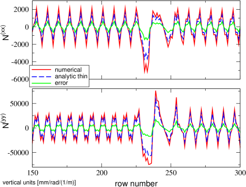
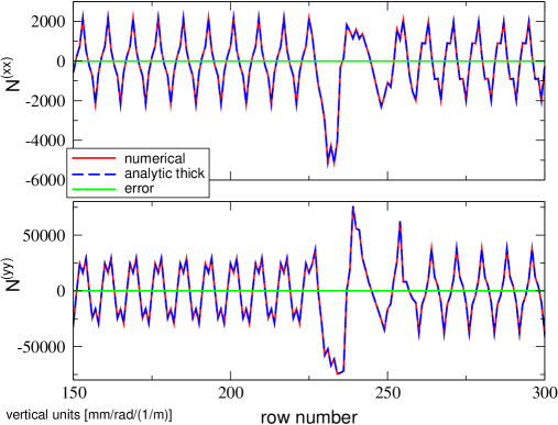
Figure 15: (Color) Example of column of the FCC-ee ORM Jacobian $N$ computed numerically (red) and analytically (blue). A zoom over only 150 BPMs (among the 1600) is displayed for a better visualization. Left: the analytic $N$ is computed in the thin-lens approximation with constant optical parameters, yielding a sizeable discrepancy (green curve). Right: the analytic solution is computed by replacing the optical functions by the corresponding integrals of the previous sections, showing an almost perfect agreement.

  

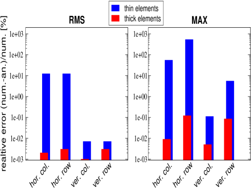
Figure 16: (Color) Right: Same plot as the right chart of Fig. 15 with the difference between numerical and analytical solution multiplied by $10^{4}$ in order to visualize the residual difference. Left: rms and maximum relative difference from the (true) numerical response and the analytical ones computed along both the matrix columns and rows.

As global figures of merit to asses the increase in accuracy for the entire Jacobian $N$, the rms and maximum relative difference from the (true) numerical response and the analytical ones have been computed along both the matrix columns and rows. The left plot of Fig. 16 shows the results, confirming the substantial gain in accuracy provided by these corrections.

C.9 Corrections for the tune shift induced by a quadrupolar error

The standard first-order formula used to evaluate the betatron tune shift $\Delta Q$ induced by quadrupole excitation $\Delta K_{m}$ reads Zimmermann-book

$$\frac{\Delta Q_{q}}{\Delta K_{m}}=\pm\frac{\beta_{q,m}}{4\pi}\ ,\hskip 28.45274pt\hbox{with }\ q=x,y\ ,$$ (612)

where the $\pm$ sign refers to the horizontal and vertical planes, respectively. The beta function is here considered as its mean value across the quadrupole $m$. We can thus replace it with the integral $I_{\beta,m}$ defined in Eq. (527) and evaluated via Eq. (547) in both planes.

$$\frac{\Delta Q_{q}}{\Delta K_{m}}=\pm\frac{I_{\beta_{q},m}}{4\pi}\ .$$ (613)

Even though the above equation remains a first-order (improved) approximation, its accuracy increases dramatically. A test was carried out with the lattice of the ESRF EBS by varying one focusing quadrupole by $\Delta K_{m}=1^{-4}$ 1/m. The relative error $\delta_{q}=\left(\Delta Q_{q}^{\hbox{(true)}}-\Delta Q_{q}^{\hbox{(formula)}}\right)/\Delta Q_{q}^{\hbox{(true)}}$ in evaluating the tune shifts with the two formulas were

$$\left\{\begin{aligned} \delta_{x}&=-5.9\%\\ \delta_{y}&=12.8\%\end{aligned}\right.\hskip 28.45274pt\hbox{with Eq.~{}\eqref{eq:tuneshift1}}\ ,\qquad\left\{\begin{aligned} \delta_{x}&=<10^{-3\ }\%\\ \delta_{y}&=<10^{-3\ }\%\end{aligned}\right.\hskip 28.45274pt\hbox{with Eq.~{}\eqref{eq:tuneshift2}}\ ,$$ (614)

which is dramatic, despite the fact that Eq. (613) remains a first-order approximation.

C.10 Correction for the coupling and focusing RDTs

All the above integrals accounting for the variation of the optical functions across magnets improve dramatically the accuracy of the analytic formulas for the ORM, chromatic functions and tune shift. It is therefore natural to explore their impact in the evaluation of the coupling and focusing RDTs from the analytic formulas to first order

$$f_{2000,j} = -\frac{\sum\limits_{m=1}^{M}\delta K_{m,1}\beta_{m,x}e^{2i\Delta\phi_{x,mj}}}{8(1-e^{4\pi iQ_{x}})}\ ,\hskip 59.75095ptf_{0020,j}=+\frac{\sum\limits_{m=1}^{M}\delta K_{m,1}\beta_{m,y}e^{2i\Delta\phi_{y,mj}}}{8(1-e^{4\pi iQ_{y}})}\ ,$$

$$f_{1001,\j} = \frac{\sum\limits_{m=1}^{M}J_{m,1}\sqrt{\beta_{m,x}\beta_{m,y}}e^{i(\Delta\phi_{x,mj}-\Delta\phi_{y,mj})}}{4(1-e^{2\pi i(Q_{u}-Q_{v})})}\ ,\quad f_{1010,\j}=\frac{\sum\limits_{m=1}^{M}J_{m,1}\sqrt{\beta_{m,x}\beta_{m,y}}e^{i(\Delta\phi_{x,mj}+\Delta\phi_{y,mj})}}{4(1-e^{2\pi i(Q_{u}+Q_{v})})}\ ,$$

(615)

where $j$ denotes the usual generic location. The above definitions assume thin quadrupoles (normal and skew) or constant optical parameters $\beta$ and $\phi$. In order to account for their variation across the magnets, the following terms need to be replaced by their integrals

$$\beta_{m,q}e^{2i\Delta\phi_{q,mj}}\quad \rightarrow \quad R_{m,j}^{(2,q)}=\frac{1}{L_{m}}\int_{0}^{L_{m}}{\beta_{q}(s)e^{2i\Delta\phi(s)_{q,j}}ds},\hskip 28.45274pt\hbox{with }\ q=x,y\ ;$$ (616)

$$\sqrt{\beta_{m,x}\beta_{m,y}}e^{i(\Delta\phi_{x,mj}\pm\Delta\phi_{y,mj})}\quad \rightarrow \quad R_{m,j}^{(11,\pm)}=\frac{1}{L_{m}}\int_{0}^{L_{m}}{\sqrt{\beta_{x}(s)\beta_{y}(s)}e^{i[\Delta\phi(s)_{x,m}\pm\Delta\phi(s)_{y,m}]}\ ds}\ .$$ (617)

The positive sign in the latter refers to the RDT $f_{1010}$, while the negative to $f_{1001}$. All ingredients to evaluate the above integrals have been already derived in the previous sections. Indeed, the left term of Eq. (616) reads

$$\beta_{m,q}e^{2i\Delta\phi_{q,mj}}=\beta_{m,q}[\cos{(2\Delta\phi_{x,mj})}+i\sin{(2\Delta\phi_{x,mj})}]\ ,$$ (618)

which comprises the same integrals of Eqs. (528), (529) and (548), after replacing the shifted phase advance between the location $j$ and the entrance of the magnet $m$, $\tau_{s_{m}j}$, with the standard (unshifted) phase advance $\Delta\phi_{s_{m}j}$.

$$\begin{aligned} \beta_{m,q}\sin{(2\Delta\phi_{x,mj})}&\rightarrow\sin{(2\Delta\phi_{s_{m}j})}I_{C,m}-\cos{(2\Delta\phi_{s_{m}j})}I_{S,m}\quad,\quad I_{C,m}=\frac{1}{L_{m}}\int_{0}^{L_{m}}{\beta(s)\cos{(2\Delta\phi_{s})}_{\ }ds}\ ,\\ \beta_{m,q}\cos{(2\Delta\phi_{x,mj})}&\rightarrow\cos{(2\Delta\phi_{s_{m}j})}I_{C,m}+\sin{(2\Delta\phi_{s_{m}j})}I_{S,m}\quad,\quad I_{S,m}=\frac{1}{L_{m}}\int_{0}^{L_{m}}{\beta(s)\sin{(2\Delta\phi_{s})}_{\ }ds}\ .\end{aligned}$$ (619)

By insetting Eq. (619) into Eq. (618) and the latter into Eq. (616), we obtain

$$R_{m,j}^{(2)}=\cos{(2\Delta\phi_{s_{m}j})}\left[I_{C,m}-iI_{S,m}\right]+\sin{(2\Delta\phi_{s_{m}j})}\left[I_{S,m}+iI_{C,m}\right]\ ,$$ (620)

where $I_{C,m}$ and $I_{S,m}$ for quadrupoles are defined in Eqs. (549) and (550), respectively. The plane label $q=x,y$ has been omitted here for sake of notation, though the above expression shall be evaluated in the horizontal plane for $f_{2000}$ and in the vertical for $f_{0020}$, since

$$f_{2000,j}=-\frac{\sum\limits_{m=1}^{M}\delta K_{m,1}R_{m,j}^{(2,x)}}{8(1-e^{4\pi iQ_{x}})}\quad,\hskip 31.2982ptf_{0020,j}=+\frac{\sum\limits_{m=1}^{M}\delta K_{m,1}R_{m,j}^{(2,y)}}{8(1-e^{4\pi iQ_{y}})}\ .\quad$$ (621)

The coupling terms $R_{m,j}^{(11,\pm)}$ require a bit of trigonometric gymnastics in order to isolate and evaluate the integrals across the quadrupole length. The first step is

$$e^{i(\Delta\phi_{x,mj}\pm\Delta\phi_{y,mj})}= \ \cos{(\Delta\phi_{x,mj}\pm\Delta\phi_{y,mj})}+i\sin{(\Delta\phi_{x,mj}\pm\Delta\phi_{y,mj})}$$

$$= \hskip 14.22636pt\left[\cos{(\Delta\phi_{x,mj})}\cos{(\Delta\phi_{y,mj})}\mp\sin{(\Delta\phi_{x,mj})}\sin{(\Delta\phi_{y,mj})}\right]$$ (622)

$$+i\left[\sin{(\Delta\phi_{x,mj})}\cos{(\Delta\phi_{y,mj})}\pm\cos{(\Delta\phi_{x,mj})}\sin{(\Delta\phi_{y,mj})}\right]\ .$$

By replacing the constant terms with their integrals

$$\begin{aligned} \sqrt{\beta_{m,q}}\sin{(\Delta\phi_{q,mj})}\ &\rightarrow\ M_{S,mj}^{(q)}=\frac{1}{L_{m}}\int_{0}^{L_{m}}{\sqrt{\beta_{q}(s)}\sin{[\Delta\phi_{q,j}(s)]}_{\ }ds}\\ \sqrt{\beta_{m,q}}\cos{(\Delta\phi_{q,mj})}\ &\rightarrow\ M_{C,mj}^{(q)}=\frac{1}{L_{m}}\int_{0}^{L_{m}}{\sqrt{\beta_{q}(s)}\cos{[\Delta\phi_{q,j}(s)]}_{\ }ds}\end{aligned}\ ,$$ (623)

it turns out that the above integrals are similar to the ones of Eqs. (530) and (531), after replacing the shifted phase advance between the location $j$ and the entrance of the magnet $m$, $\tau_{s_{m}j}$, with the standard (unshifted) phase advance $\Delta\phi_{s_{m}j}$. They are then computed by applying the same derivation of Sec. C.4, yielding

$$\begin{aligned} M_{S,mj}&=\sin{(\Delta\phi_{s_{m}j})}G_{C,m}-\cos{(\Delta\phi_{s_{m}j})}G_{S,m}\quad,\\ M_{C,mj}&=\cos{(\Delta\phi_{s_{m}j})}G_{C,m}+\sin{(\Delta\phi_{s_{m}j})}G_{S,m}\quad,\end{aligned}$$ (624)

where $G_{S,m}$ and $G_{C,m}$ are the same of Eq. (569) and shall be evaluated for both planes, whose label $q=x,y$ has been dropped here for sake of notation. By replacing Eq. (623) into Eq. (622) the coupling terms $R_{m,j}^{(11,\pm)}$ read

$$R_{m,j}^{(11,\pm)}=M_{C,mj}^{(x)}M_{C,mj}^{(y)}\mp M_{S,mj}^{(x)}M_{S,mj}^{(y)}+i\left[M_{S,mj}^{(x)}M_{C,mj}^{(y)}\pm M_{C,mj}^{(x)}M_{S,mj}^{(y)}\right]\ ,$$ (625)

and the RDTs

$$f_{1001,\j}=\frac{\sum\limits_{m=1}^{M}J_{m,1}R_{m,j}^{(11,-)}}{4(1-e^{2\pi i(Q_{u}-Q_{v})})}\quad,\hskip 31.2982ptf_{1010,\j}=\frac{\sum\limits_{m=1}^{M}J_{m,1}R_{m,j}^{(11,+)}}{4(1-e^{2\pi i(Q_{u}+Q_{v})})}\ .\quad$$ (626)

C.11 Inferring the focusing and coupling RDTs from the one-turn matrix

RDTs are usually either computed from the analytic formulas presented in the previous section, or extracted from the harmonic analysis of turn-by-turn data (see Ref. Andrea-Linear-arxiv and references therein). Additionally, coupling RDTs can be inferred from the coupling matrix $\mathbf{C}$, which in turn is derived from the one-turn matrix, as discussed in Ref. merging . This multitude of sources allows a handy crosscheck of any code implementation to evaluate them. In this section we derive yet another way to compute the RDTs directly from the one-turn matrix (OTM). The focusing RDTs $f_{2000}$ and $f_{0020}$ will be inferred from the difference between the ideal on-diagonal blocks of the OTM and the one obtained after including focusing errors. The off-diagonal blocks will be instead used to extract the coupling RDTs $f_{1001}$ and $f_{1010}$.

The starting point the OTM in Cartesian coordinates $\mathbf{M}$ at an arbitrary location along the ring, which is the one readily available in output of optics codes such as MADX or Accelerator Toolbox:

$$\vec{X}^{(N+1)}=\mathbf{M}\vec{X}^{(N)}\ ,\qquad\vec{X}=\left(\begin{array}[]{c}x\\ p_{x}\\ y\\ p_{y}\end{array}\right)\quad,\quad$$ (631)

where $N$ denotes a generic turn. The OTM $\mathbf{M}$ is a 4x4 matrix with non-zero off-diagonal blocks, which differs from the ideal block-diagonal 4x4 OTM $\mathbf{M_{0}}$.

In the normal form coordinates $\vec{\zeta}$ of Eq. (157), the OTM is a diagonal matrix describing a pure rotation defined by the eigen-tunes (which correspond to the betatron tunes as long as the they are sufficiently far away from the resonance stop-band prstab_coup ) $e^{i\mathbf{Q}}=\hbox{diag}(e^{2\pi iQ_{x}},e^{-2\pi iQ_{x}},e^{2\pi iQ_{y}},e^{-2\pi iQ_{y}})$ of Eq. (173):

$$\vec{\zeta}^{(N+1)}=e^{i\mathbf{Q}}\vec{\zeta}^{(N)}\ ,\qquad\vec{\zeta}^{(N)}=\left(\begin{array}[]{c}\zeta_{x,-}\\ \zeta_{x,+}\\ \zeta_{y,-}\\ \zeta_{y,+}\end{array}\right)\quad.$$ (636)

By walking through the three changes of coordinates that transform the Cartesian vector in the one in normal form, the relation between the RDTs and the OTM $\mathbf{M}$ will be derived. The first step is the standard Courant-Snyder (C-S) transformation matrix $\mathbf{C}$

$$\vec{\tilde{X}}=\mathbf{C}\vec{X}\quad,\quad\mathbf{C}=\left(\begin{array}[]{c c c c }\displaystyle\frac{1}{\sqrt{\beta_{x}}}&0&0&0\\ \displaystyle\frac{\alpha_{x}}{\sqrt{\beta_{x}}}&\displaystyle\sqrt{\beta_{x}}&0&0\\ 0&0&\displaystyle\frac{1}{\sqrt{\beta_{y}}}&0\\ 0&0&\displaystyle\frac{\alpha_{y}}{\sqrt{\beta_{y}}}&\displaystyle\sqrt{\beta_{y}}\end{array}\right)\quad\Rightarrow\quad\qquad\quad$$ (641)

$$\quad\Rightarrow\quad\left(\mathbf{C^{-1}}\vec{\tilde{X}}^{(N+1)}\right)=\mathbf{M}\left(\mathbf{C^{-1}}\vec{\tilde{X}}^{(N)}\right)\quad\Rightarrow\quad\vec{\tilde{X}}^{(N+1)}=\left(\mathbf{C}\mathbf{M}\mathbf{C^{-1}}\right)\vec{\tilde{X}}^{(N)}\quad.$$ (642)

The second step is to move from the real C-S to the complex C-S coordinates $h_{z,\pm}=\tilde{z}\pm i\tilde{p}_{z}$ of Eq. (157)

$$\vec{h}=\mathbf{T}\vec{\tilde{X}}\quad,\quad\mathbf{C}=\vec{h}=\left(\begin{array}[]{c}h_{x,-}\\ h_{x,+}\\ h_{y,-}\\ h_{y,+}\end{array}\right)\quad,\quad\mathbf{T}=\left(\begin{array}[]{c c c c }1&-i&0&0\\ 1&+i&0&0\\ 0&0&1&-i\\ 0&0&1&+i\end{array}\right)\quad\Rightarrow\quad\qquad\qquad$$ (651)

$$\quad\Rightarrow\quad\left(\mathbf{T^{-1}}\vec{h}^{(N+1)}\right)=\left(\mathbf{C}\mathbf{M}\mathbf{C^{-1}}\right)\left(\mathbf{T^{-1}}\vec{h}^{(N)}\right)\quad\Rightarrow\quad\vec{h}^{(N+1)}=\left(\mathbf{T}\mathbf{C}\mathbf{M}\mathbf{C^{-1}}\mathbf{T^{-1}}\right)\vec{h}^{(N)}\quad.$$ (652)

Note that $\mathbf{T}$ is not symplectic, each diagonal block having a determinant equal to 1/2. The last step is to eventually move into normal form via the transformation of Eq. (167)

$$\vec{\zeta}=\mathbf{B}\vec{h}+O(f^{2})\quad,\quad\mathbf{B}=\left(\begin{array}[]{c c c c}1&4if_{2000}&\ \ 2if_{1001}&\ \ 2if_{1010}\\ -4if_{2000}^{*}&1&-2if_{1010}^{*}&-2if_{1001}^{*}\\ \ \ 2if_{1001}^{*}&\ \ 2if_{1010}&1&\ \ 4if_{0020}\\ -2if_{1010}^{*}&-2if_{1001}&-4if_{0020}^{*}&1\end{array}\right)\ +O(f^{2})\quad\Rightarrow\quad\qquad\qquad$$ (657)

$$\quad\Rightarrow\quad\left(\mathbf{B^{-1}}\vec{\zeta}^{(N+1)}\right)=\left(\mathbf{T}\mathbf{C}\mathbf{M}\mathbf{C^{-1}}\mathbf{T^{-1}}\right)\left(\mathbf{B^{-1}}\vec{\zeta}^{(N)}\right)\quad\Rightarrow\quad\vec{\zeta}^{(N+1)}=\left(\mathbf{B}\mathbf{T}\mathbf{C}\mathbf{M}\mathbf{C^{-1}}\mathbf{T^{-1}}\mathbf{B^{-1}}\right)\vec{\zeta}^{(N)}\quad.$$ (658)

Since the last relation in the above equation must be equal to the first of Eq. (636), we can write

$$e^{i\mathbf{Q}}=\mathbf{B}\mathbf{T}\mathbf{C}\mathbf{M}\mathbf{C^{-1}}\mathbf{T^{-1}}\mathbf{B^{-1}}\quad\Rightarrow\quad\mathbf{M}=\mathbf{C^{-1}}\mathbf{T^{-1}}\mathbf{B^{-1}}e^{i\mathbf{Q}}\mathbf{B}\mathbf{T}\mathbf{C}\ .$$ (659)

Interestingly, even though four complex matrices appear in the r.h.s. of the last equation, namely $\mathbf{T^{-1}},\ \mathbf{B^{-1}},\ e^{i\mathbf{Q}},\ \mathbf{B}$ and $\mathbf{T}$, the entire r.h.d. must be a real 4x4 matrix which in the limit of no focusing errors (i.e. $f_{2000}=f_{0020}=0$) and of no coupling (i.e. $f_{1001}=f_{1010}=0$) shall be equal to the ideal OTM

$$\mathbf{M_{0}}=\left(\begin{array}[]{c c c c}\cos{\mu_{x}}+\alpha_{x}\sin{\mu_{x}}&\beta_{x}\sin{\mu_{x}}&0&0\\ -\gamma_{x}\sin{\mu_{x}}&\cos{\mu_{x}}-\alpha_{x}\sin{\mu_{x}}&0&0\\ 0&0&\cos{\mu_{y}}+\alpha_{y}\sin{\mu_{y}}&\beta_{y}\sin{\mu_{y}}\\ 0&0&-\gamma_{y}\sin{\mu_{y}}&\cos{\mu_{y}}-\alpha_{y}\sin{\mu_{y}}\end{array}\right)\quad,\quad$$ (664)

where $\mu=2\pi Q$ and $\gamma=(1+\alpha^{2})/\beta$.

Two intermediary steps will help deriving more accurate and readable formulas for the focusing RDTs. The first step is to actually develop the last relation of Eq. (659) in the C-S rather than Cartesian coordinates, namely

$$\mathbf{\tilde{M}}=\mathbf{T^{-1}}\mathbf{B^{-1}}e^{i\mathbf{Q}}\mathbf{B}\mathbf{T}\ ,\quad\hbox{where }\quad\mathbf{\tilde{M}}=\mathbf{C}\mathbf{M}\mathbf{C^{-1}}\ .$$ (665)

The second step is to replace the first-order transformation $\mathbf{B}$ of Eq. (657) with one including all orders of the focusing RDTS $f_{2000}$ and $f_{0020}$, while keeping the coupling part truncated to the first order. Even though analytic formulas including all orders of the coupling RDTs do exist (see Appendix A of Ref. prstab_esr_coupling and Appendix C of Ref. Sext-RDT ), they have been derived assuming no focusing error. The cross-talk between higher order focusing and coupling RDTs renders more general analytic expressions cumbersome to derive and to write. For this reason, the priority is given here to an all-order analysis of focusing RDTs, while keeping the coupling part truncated to first order, i.e. to weak coupling ($|f_{1001}|,|f_{1010}|\ll|f_{2000}|,|f_{0020}|$) with tunes outside the coupling stop-bands ($|Q_{x}\pm Q_{y}|\gg|C_{\pm}|$). By making use of Eqs.(C8) and (C9) of Ref. Sext-RDT ), the transformation matrix $\mathbf{B}$ can be written as

$$\mathbf{B}=\left(\begin{array}[]{c c}\mathbf{B_{xx}}&\mathbf{B_{xy}}\\ \mathbf{B_{yx}}&\mathbf{B_{yy}}\end{array}\right)\quad,\qquad\mathbf{B_{xx}}=\left(\begin{array}[]{c c}\cosh{(4|f_{2000}|)}&i\sinh{(4|f_{2000}|)}e^{iq_{2000}}\\ -i\sinh{(4|f_{2000}|)}e^{iq_{2000}}&\cosh{(4|f_{2000}|)}\end{array}\right)\ ,$$ (670)

where $q_{2000}=\hbox{arg}\{f_{2000}\}$ is the RDT phase. The vertical diagonal block $\mathbf{B_{yy}}$ comprises the same elements, after replacing $f_{2000}$ with $f_{0020}$. The off-diagonal blocks $\mathbf{B_{xy}}$ and $\mathbf{B_{xy}}$ are the same first-order truncated expression of Eq. (657).

By making explicit the r.h.s of the first relation in Eq. (665), the horizontal diagonal block of the OTM in C-S coordinates reads

$$\mathbf{\tilde{M}}=\mathbf{\tilde{M_{0}}}+\mathbf{\delta\tilde{M}}\quad,\quad\mathbf{\tilde{M_{0}}}=\left(\begin{array}[]{c c}\Re\{e^{i\mu_{x}}\}&\Im\{e^{i\mu_{x}}\}\\ -\Im\{e^{i\mu_{x}}\}&\Re\{e^{i\mu_{x}}\}\end{array}\right)\quad,\hskip 113.81102pt$$ (673)

$$\mathbf{\tilde{\delta M}}=\sin{\mu_{x}}\left(\begin{array}[]{c c}-\sinh{(8|f_{2000}|)}\cos{q_{2000}}&2\sinh^{2}{(4|f_{2000}|)}+\sinh{(8|f_{2000}|)}\sinh{q_{2000}}\\ -2\sinh^{2}{(4|f_{2000}|)}+\sinh{(8|f_{2000}|)}\sinh{q_{2000}}&\sinh{(8|f_{2000}|)}\cos{q_{2000}}\end{array}\right)\ .\quad$$ (676)

$\mathbf{\tilde{M_{0}}}$ is the unperturbed ideal OTM in C-S coordinates, whereas $\mathbf{\delta\tilde{M}}$ is the difference between the actual and the ideal OTM in C-S coordinates. The latter represents the observable, as it can be computed by any optics code. Other higher-order terms stemming from the normal form transformations (not discussed here, but derivable from Appendix A of Ref. Sext-RDT )) generate phase-independent terms in the matrix $\mathbf{\delta\tilde{M}}$ which are not accounted for here. A simple, though not perfect, way to remove their contribution is to evaluate the average of $\mathbf{\delta\tilde{M}}$ along the ring circumference $C$ and to subtract it from $\mathbf{\delta\tilde{M}}$, so to have only phase-dependent terms and to be more consistent with the present scheme, namely

$$\mathbf{\delta\tilde{M}}\rightarrow\mathbf{\delta\tilde{M}}-<\mathbf{\delta\tilde{M}}>\quad,\quad\hbox{where}\quad<\mathbf{\delta\tilde{M}}>=\frac{1}{C}\oint{\mathbf{\delta\tilde{M}}(s)\ ds}\ .$$ (677)

This manipulation is sufficient in the presence of a single quadrupole error, i.e. with $|f_{2000}|$ constant along the ring, and thus in the evaluation of any RDT response matrix, though for a more generic lattice with distributed quadrupole errors (and possibly coupling), the resulting variation of $|f_{2000}|$ along the ring would still introduce an error, which can be estimated by the later Eq. (679).

The system of Eq. (676) provides the following relations for the horizontal focusing RDT

$$\begin{aligned} |f_{2000}|&=\frac{1}{8}\sinh^{-1}{\Biggl{(}\frac{\sqrt{(\delta\tilde{M}_{12}+\delta\tilde{M}_{21})^{2}+4\delta\tilde{M}_{11}^{2}}}{2\sin{\mu_{x}}}\ \Biggr{)}}\ ,\\ \cos{q_{2000}}&=\frac{-2\delta\tilde{M}_{11}}{\sqrt{(\delta\tilde{M}_{12}+\delta\tilde{M}_{21})^{2}+4\delta\tilde{M}_{11}^{2}}}\ ,\\ \sin{q_{2000}}&=\frac{\delta\tilde{M}_{12}+\delta\tilde{M}_{21}}{\sqrt{(\delta\tilde{M}_{12}+\delta\tilde{M}_{21})^{2}+4\delta\tilde{M}_{11}^{2}}}\ ,\end{aligned}$$ (678)

where $\sinh^{-1}{(x)}=\log{(\sqrt{x^{2}+1})}+x$ is the inverse hyperbolic function. The above expressions suffice to compute both the imaginary and real parts of $f_{2000}$ a any location. Equation (676) provides also a relation that shall be satisfied by $\mathbf{\tilde{\delta M}}$ which in turn can be used to estimate the accuracy in the above calculations, namely

$$0\simeq\hbox{Err}=\left|\frac{\delta\tilde{M}_{11}+\delta\tilde{M}_{22}}{16\sin{\mu_{x}}}\right|\ll|f_{2000}|\ .$$ (679)

By inserting Eq. (673) into the right expression of Eq. (665) the matrix elements $\delta\tilde{M}_{ij}$ are readily computed from the C-S unperturbed parameters and the difference between the actual and unperturbed (or ideal) OTMs in Cartesian coordinates, $\mathbf{\delta M}$, both to be computed by any optics code:

$$\left\{\begin{aligned} \delta\tilde{M}_{11}&=\delta M_{11}-\frac{\alpha_{x}}{\beta_{x}}\delta M_{12}\\ \delta\tilde{M}_{12}&=\alpha_{x}\delta M_{11}-\frac{\alpha_{x}^{2}}{\beta_{x}}\delta M_{12}+\beta_{x}\delta M_{21}-\alpha_{x}\delta M_{22}\\ \delta\tilde{M}_{21}&=\frac{1}{\beta_{x}}\delta M_{21}\\ \delta\tilde{M}_{22}&=\frac{\alpha_{x}}{\beta_{x}}\delta M_{12}+\delta M_{22}\end{aligned}\right.\quad.$$ (680)

It is reminded that the subtraction of Eq. (677) shall be performed prior to the insertion of the above terms into Eq. (678).

The same considerations applied to the vertical diagonal block yields to the following relations for the focusing RDT $f_{0020}$:

$$\begin{aligned} |f_{0020}|&=\frac{1}{8}\sinh^{-1}{\Biggl{(}\frac{\sqrt{(\delta\tilde{M}_{34}+\delta\tilde{M}_{43})^{2}+4\delta\tilde{M}_{33}^{2}}}{2\sin{\mu_{y}}}\ \Biggr{)}}\ ,\\ \cos{q_{0020}}&=\frac{-2\delta\tilde{M}_{33}}{\sqrt{(\delta\tilde{M}_{34}+\delta\tilde{M}_{43})^{2}+4\delta\tilde{M}_{33}^{2}}}\ ,\\ \sin{q_{0020}}&=\frac{\delta\tilde{M}_{34}+\delta\tilde{M}_{43}}{\sqrt{(\delta\tilde{M}_{34}+\delta\tilde{M}_{43})^{2}+4\delta\tilde{M}_{33}^{2}}}\ ,\end{aligned}$$ (681)

with the same error estimation

$$0\simeq\hbox{Err}=\left|\frac{\delta\tilde{M}_{33}+\delta\tilde{M}_{44}}{\sin{\mu_{y}}}\right|\ll|f_{0020}||\ ,$$ (682)

and computation of $\mathbf{\delta\tilde{M}_{yy}}$

$$\left\{\begin{aligned} \delta\tilde{M}_{33}&=\delta M_{33}-\frac{\alpha_{y}}{\beta_{y}}\delta M_{34}\\ \delta\tilde{M}_{34}&=\alpha_{y}\delta M_{33}-\frac{\alpha_{y}^{2}}{\beta_{y}}\delta M_{34}+\beta_{y}\delta M_{43}-\alpha_{y}\delta M_{44}\\ \delta\tilde{M}_{43}&=\frac{1}{\beta_{y}}\delta M_{43}\\ \delta\tilde{M}_{44}&=\frac{\alpha_{y}}{\beta_{y}}\delta M_{34}+\delta M_{44}\end{aligned}\right.\quad.$$ (683)

In Fig. 17 an example of different computations of $f_{2000}$ at the 224 BPMs of the old ESRF storage ring, with a single error at a focusing quadrupole is shown. The RDT is calculated from the lattice formula of Eq. (615) (black), from the FFT of single particle tracking data and Eq.(C8) of Ref. Sext-RDT (green) and from the OTM via Eq. (678). The error functions $\hbox{Err}_{\Re}$ (left plot) and $\hbox{Err}_{\Im}$ (right plot) are displayed in blue, indicating an excellent applicability of the OTM formulas. The agreement between the lattice and OTM formulas is indeed remarkable. Analogous results are obtained for $f_{0020}$ (not shown here).

In order to explore the range of validity of the OTM formulas and the pollution introduced by betatron coupling, the same computation has been carried out after including a typical linear lattice error model comprising distributed quadrupole errors and sources of coupling. Results for $f_{2000}$ are shown in Fig. 18 (similar results apply to $f_{0020}$, not shown here). The agreement between the different formulas is poorer, and the sizeable amplitude of the error function $\hbox{Err}_{\Im}$ (blue curve, right plot), casts doubts on the accuracy of the derivation of the focusing RDTs from the OTM.

      

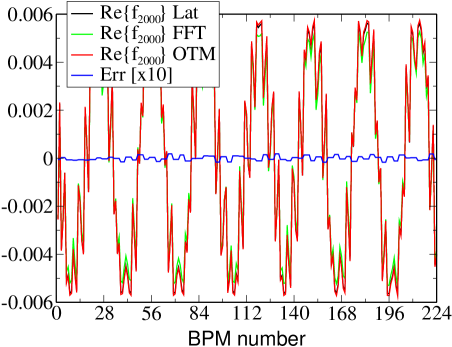
Figure 17: (Color) Example of different computations of $f_{2000}$ at the 224 BPMs of the old ESRF storage ring, with a single error at a focusing quadrupole: from the lattice formula of Eq. (615) (black), from the FFT of single particle tracking data and Eq.(C8) of Ref. Sext-RDT (green) and from the OTM via Eq. (678). The error function Err is displayed too (blue, multiplied by 10), indicating an excellent applicability of the OTM formulas.

      

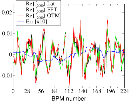
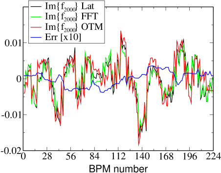
Figure 18: (Color) Same plot of Fig. 17 but with a realistic error model of the old ESRF storage ring comprising distributed focusing errors and sources of betatron coupling. The latter corrupt the possibility of inferring accurately the focusing RDTs from the OTM, as suggested by the sizeable error function Err (blue, multplied by 10).

References

- (1) M. Minty and F. Zimmermann, Measurement and Control of Charged Particle Beams, Springer, Berlin, 2003 (ISBN 3-540-44197-5).
- (2) R. Tomás, M. Aiba, A. Franchi, U. Iriso, Phys. Rev. Accel. Beams, vol. 20, 054801, (2017).
- (3) J. Safranek, Nucl. Instr. and Meth. A, vol. 388, pp. 27-36 (1996).
- (4) ICFA BD Newsletter, edited by A. Ghodke (ICFA Beam Dynamics Panel, 2007), No. 44 .
- (5) S. M. Liuzzo, PhD Thesis, University of Roma Tor Vergata, 2013 (unpublished).
- (6) G. Rehm, M.G. Abbott, A.F. D. Morgan, J. Rowland, I. Uzun, Proceedings of Beam and Instrumentation Workshop BIW2010, Santa Fe, New Mexico USA, 2010.
- (7) X. Yang, V. Smaluk, L. H. Yu, Y. Tian, and K. Ha, Phys. Rev. Accel. Beams, vol. 20, 054001, (2017).
- (8) W. Herr, F. Schmidt, CERN AB Note, CERN-AB-2004-027-ABP (2004).
- (9) A. Terebilo, Proceedings of PAC01, p 3203, Chicago, Illinois, USA (2001).
- (10) A. Franchi, L. Farvacque, J. Chavanne, F. Ewald, B. Nash, K. Scheidt and R. Tomás, Phys. Rev. ST Accel. Beams, vol. 14, 034002, (2011).
- (11) A. Franchi, http://arxiv.org/abs/1603.00281
- (12) A. Franchi, L. Farvacque, F. Ewald, G. Le Bec and K. B. Scheidt, http://arxiv.org/abs/1402.1461. A. Franchi, L. Farvacque, F. Ewald, G. Le Bec and K. B. Scheidt, Phys. Rev. ST Accel. Beams, vol. 17, 074001, (2013).
- (13) J. Bengtsson and J. Irwin, Analytical calculation of smear and tune shift, SSC Note, SSC-232, Berkeley, CA, (1990)
- (14) Y. Luo, S. Tepikian, W. Fischer, G. Robert-Demolaize, D. Trbojevic, Sorting chromatic sextupoles for easily and effectively correcting second order chromaticity in the Relativistic Heavy Ion Collider, Note C-A/AP/348 (2009).
- (15) V. Lebedev and V. D. Shiltsev (editors), Accelerator Physics at the Tevatron Collider, Springer, Berlin, 2016 (ISBN 1493908855)
- (16) A. Franchi, E. Métral, and R. Tomás García, Phys. Rev. ST Accel. Beams, vol. 10, 064003 (2007).
- (17) R.Calaga, R. Tomás, and A. Franchi, Phys. Rev. ST Accel. Beams 8, 034001 (2005).
- (18) A. Franchi, L. Farvacque, F. Ewald, G. Le Bec and K. B. Scheidt, http://arxiv.org/abs/1402.1461 (2013).