Random walk on a randomly oriented honeycomb lattice

Abstract.

We study the recurrence behaviour of random walks on partially oriented honeycomb lattices. The vertical edges are undirected while the orientation of the horizontal edges is random: depending on their distribution, we prove a.s. transience in some cases, and a.s. recurrence in other ones. The results extend those obtained for the partially oriented square grid lattices (Campanino and Petritis (2003), Campanino and Petritis (2014)).

1. Introduction

1.1. Motivation

The behaviour of random walks on oriented two-dimensional graphs has been object in the last years of several works. In particular new methods have to be devised to settle the question of their recurrence or transience. The main result of Campanino and Petritis (2003) concerns the random walk on the two-dimensional square lattice where the vertical edges are undirected while the edges on each horizontal line are all oriented randomly and independently to the right or to the left with equal probability. The result is that this random walk is transient almost surely with respect to the environment; in Campanino and Petritis (2014) the study is generalized to a more general class of environments, in particular showing that the random walk is recurrent provided that the lines are oriented through periodic functions. In the last decade many authors have investigated this and related models: just to cite some of them, in Guillotin-Plantard and Le Ny (2008) a functional limit theorem for the random walk is proved, in Castell et al. (2011) a local limit theorem is established, and in Guillotin-Plantard and Pène (2015) the range of the walk is analyzed; in Pène (2009) the author considers the case where the lines are oriented by a sequence of stationary random variables, while in Devulder and Pène (2013) the model is generalized to one where the probability of staying on a line is non-constant. A common characteristic of the considered random walks is that one can split them, apart from a time change, into a “horizontal” and “vertical” component, where the latter is independent from the former. Moreover all these studies deal with the square grid lattice, and one can ask if these recurrence properties still hold as the geometry of the underlying two-dimensional graph changes: motivated by this question, in the present work we consider the random walk on the honeycomb randomly directed lattice. Here the “vertical motion” obtained from the splitting is no longer independent from the “horizontal” one: as a result, the subsequent steps of the “vertical motion” have a markovian dependency. For this reason, while some of the techniques used in Campanino and Petritis (2003) and Campanino and Petritis (2014) can be properly extended and adopted in our study, in several parts of the proof we need to develop new ideas and techniques. While we consider just a specific example also for reasons of simplicity, we expect in the future to be able to extend our approach to a more general setting.

1.2. Notation and results

Let $\mathbf{L}:=(\mathbb{Z}^{2},E)$ be the square grid lattice, i.e. $E$ is the set of nearest neighbours in $\mathbb{Z}^{2}$. The honeycomb lattice can be defined as the sub-graph obtained from $\mathbf{L}$ by eliminating the following set of edges (see figure 1.1)

$$\{((2j,2k),(2j,2k+1))|\,j,k\in\mathbb{Z}\}$$

$$\cup \{((2j,2k+1),(2j,2k))|\,j,k\in\mathbb{Z}\}$$

$$\cup \{((2j+1,2k+1),(2j+1,2k+2))|\,j,k\in\mathbb{Z}\}$$

$$\cup \{((2j+1,2k+2),(2j+1,2k+1))|\,j,k\in\mathbb{Z}\}.$$

Then we can define partially oriented versions of the lattice by imposing a certain orientation on the horizontal edges (this can be done either deterministically or randomly), while keeping the vertical edges unoriented. Our work is devoted to the study of the recurrence (transience) behaviour of a simple random walk $(M_{n})_{n\geq 0}$ on such oriented lattices. Let $(\Omega,\mathcal{F},\mathbb{P})$ be a probability space. The first result we prove is the following:

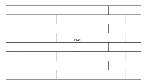
Figure 1.1. The honeycomb lattice

Theorem 1.1.

Let $(\epsilon_{y})_{y\in\mathcal{Z}}$ be a i.i.d. family of $\{-1,1\}$-valued Rademacher random variables and denote by $\mathbf{H}_{\epsilon}$ the honeycomb lattice oriented randomly as follows: if $\epsilon_{y}=1$ there is only a right-directed edge between $(x,y)$ and $(x+1,y)$, $\forall x\in\mathbb{Z}$; if $\epsilon_{y}=-1$, only a left-directed one. Then the random walk $(M_{n})_{n\geq 0}$ on $\mathbf{H}_{\epsilon}$ is a.s. transient.

Since the transience behaviour is caused by the presence and the size of fluctuations in the orientations, we impose periodic orientations and prove the following result.

Theorem 1.2.

Let $Q>1$ be an even integer and, given a $Q$-periodic function $f:\mathbb{Z}\longrightarrow\{-1,1\}$ such that $\sum_{k=0}^{Q-1}f(k)=0$, consider the oriented honeycomb lattice $\mathbf{H}_{f}$ whose horizontal edges are oriented according to the value of $f$: that is, if $f(k)=1$ then the edges with ordinate $k$ are right-directed, otherwise they are left-directed. Then the random walk $(M_{n})_{n\geq 0}$ on $\mathbf{H}_{f}$ is recurrent.

Finally, we consider the case of horizontal orientations prescribed by a random perturbation of a periodic function.

Theorem 1.3.

Let $(\epsilon_{y})_{y\in\mathbb{Z}}$ and $f$ as above and define for every $y\in\mathbb{Z}$

$$\overline{\epsilon}_{y}:=(1-\lambda_{y})f(y)+\lambda_{y}\epsilon_{y}$$

where $\lambda=(\lambda_{y})_{y\in\mathbb{Z}}$ is a $\{0,1\}$-valued sequence of independent r.v, independent of $\epsilon$ s.t.

$$\mathbb{P}(\lambda_{y}=1)=\frac{c}{|y|^{\beta}}.$$

Denote by $\mathbf{H}_{\overline{\epsilon},\lambda}$ the honeycomb lattice with such random orientations. Then

(i) If $\beta<1$, the random walk $M_{n}$ on $\mathbf{H}_{\overline{\epsilon},\lambda}$ is ($\epsilon_{y},\lambda_{y}$)-a.s. transient.

(ii) If $\beta>1$, the random walk $M_{n}$ on $\mathbf{H}_{\overline{\epsilon},\lambda}$ is ($\epsilon_{y},\lambda_{y}$)-a.s. recurrent.

2. Technical preliminaries

2.1. Decomposition of the random walk

Following Campanino and Petritis (2003), we decompose the random walk into two components that, if sampled on a particular sequence of random times, have the same recurrence behaviour of $(M_{n})$.

We begin with the following observation. Let $\xi$ be a random variable with geometric distribution of parameter $\frac{1}{2}$, and consider the event of an even or null outcome $A:=\bigcup_{m\in\mathbb{N}\cup\{0\}}\{\xi=2m\}$. We have

$$\mathbb{P}(A)=\sum_{m=0}^{\infty}\mathbb{P}(\xi=2m)=\frac{1}{2}\sum_{m=0}^{\infty}\left(\frac{1}{2}\right)^{2m}=\frac{2}{3}.$$

Obviously $\mathbb{P}(A^{c})=\frac{1}{3}$. Now, if we interpret $\xi$ as the absolute value of the first horizontal displacement of $(M_{n})$ (i.e. the number of subsequent horizontal steps before the first vertical one), we immediately see that after an odd outcome the random walk will perform a vertical down-directed step, otherwise a up-directed one. With this observation in mind, we give the following definition.

Definition 2.1.

The vertical skeleton of $(M_{n})_{n\geq 0}$ is the Markov process $(Y_{n},\nu_{n})_{n\geq 0}$ with values in $\mathbb{Z}\times\{-1,1\}$ defined by the following transition probabilities:

$$p_{(y,1),(y+1,1)}=p_{(y,-1),(y-1,-1)}=\frac{1}{3}$$

$$p_{(y,1),(y-1,-1)}=p_{(y,-1)(y+1,1)}=\frac{2}{3}$$

for any $y\in\mathbb{Z},$ and $\mathbb{P}((Y_{0},\nu_{0})=(0,1))=1.$

The first component of the vertical skeleton represents the projection on the $y$-axis of the position of the random walk, seen at the times of successive vertical steps, while the second component represents the speed -or direction- of the last step.

Remark 2.2.

By definition, the skeleton random walk $(Y_{k},\nu_{k})$ satisfies

$$Y_{k}=\sum_{i=1}^{k}\nu_{i},$$

and the transition matrix of the Markov chain $(\nu_{k})_{k\geq 0}$ has the following form:

$$\pi_{\nu}=\left(\begin{array}[]{cc}q&1-q\\ 1-q&q\end{array}\right)\text{,\,\, with }q=\frac{1}{3}.$$

Now we define the occupation measure of the vertical skeleton and the embedded random walk.

Definition 2.3.

Let $n\geq 0$. Let for every $y\in\mathbb{Z}$

$$\eta_{n}(y,\pm 1):=\sum_{k=0}^{n}\mathbf{1}_{\{(Y_{k},\nu_{k})=(y,\pm 1)\}}.$$

We define the total occupation measure $\eta_{n}$ at $y$ by

$$\eta_{n}(y):=\eta_{n}(y,1)+\eta_{n}(y,-1).$$

Definition 2.4.

Let $(\xi_{i})^{(y)}_{i\geq 0,\,y\in\mathbb{Z}}$ be a family of i.i.d. geometric random variables with parameter $p=\frac{1}{2}$, defined on $(\Omega,\mathcal{A},\mathbb{P})$. We call embedded random walk the process $(X_{n})_{n\geq 0}$ defined by

$$X_{n}:=\sum_{y\in\mathbb{Z}}\epsilon_{y}\sum_{i=1}^{\eta_{n-1}(y)}\xi_{i}^{(y)}$$

with the convention that $\sum_{i}$ vanishes whenever $\eta_{n-1}(y)=0$.

$X_{n}$ represents the abscissa of the random walk $(M_{n})_{n\geq 0}$ immediately after the $n$-th vertical movement has been performed.

Let $T_{n}=n+\sum_{y\in\mathbb{Z}}\sum_{i=1}^{\eta_{n-1}(y)}\xi_{i}^{(y)}$ be the time just after the random walk $(M_{n})$ has performed its $n$-th vertical move. Then it’s straightforward to see that $M_{T_{n}}=(X_{n},Y_{n}),$ where $(Y_{n})$ is the first component of the vertical skeleton $(Y_{n},\nu_{n}).$ Now denote by $\sigma_{n}$ the sequence of consecutive returns to $0$ of $(Y_{n})$ (by lemma 2.5 below it follows that $\sigma_{n}<\infty$ almost surely $\forall n$.) Obviously, $M_{T_{\sigma_{n}}}=(X_{\sigma_{n}},0)$.

Let $\mathcal{F}_{n}:=\sigma(\nu_{k},k\leq n)$, $\mathcal{G}:=\sigma(\epsilon_{y},y\in\mathbb{Z})$ and $\mathcal{F}\vee\mathcal{G}=\sigma(\mathcal{F}\cup\mathcal{G})$, where $\mathcal{F}=\vee_{n}\mathcal{F}_{n}$. We shall need the following lemmas.

Lemma 2.5.

As $n\to\infty$

$$\mathbb{P}_{0}(Y_{2n}=0)\sim\frac{C}{\sqrt{n}},$$

with $C>0$. In particular, $Y_{n}$ is recurrent.

Proof.

Since $Y_{2n}:=\sum_{k=1}^{2n}\nu_{k}$, the result follows by the local limit theorem for ergodic Markov chain with finite state space (see Kolmogorov (1949)). ∎

Lemma 2.6.

[Campanino and Petritis (2003), lemma 2.3] $(X_{\sigma_{n}})_{n\geq 0}$ is transient $\implies(M_{n})_{n\geq 0}$ is transient, i.e.

$$\sum_{n=0}^{\infty}\mathbb{P}_{0}(X_{\sigma_{n}}=0\mid\mathcal{F}\vee\mathcal{G})<\infty\text{ a.s }\implies\sum_{l=0}^{\infty}\mathbb{P}_{0}(M_{l}=(0,0)\mid\mathcal{G})<\infty\text{ a.s }.$$

2.2. Characteristic function of the embedded random walk

Let $n\in\mathbb{N},y\in\mathbb{Z}$ and define

$$m_{n,o}(y):=\sum_{k=0}^{n}\mathbf{1}_{\{Y_{k}=y,\nu_{k}=\nu_{k+1}\}},$$

$$m_{n,e}(y):=\sum_{k=0}^{n}\mathbf{1}_{\{Y_{k}=y,\nu_{k}\neq\nu_{k+1}\}}.$$

They satisfy $m_{n,o}(y)+m_{n,e}(y)=\eta_{n}(y).$ So we can decompose the embedded random walk $X_{n}$ as follows

$$X_{n}=\sum_{y\in\mathbb{Z}}\epsilon_{y}\left(\sum_{i=1}^{m_{n-1,o}(y)}\xi_{i,o}^{(y)}+\sum_{i=1}^{m_{n-1,e}(y)}\xi_{i,e}^{(y)}\right),$$

where $\xi_{i,o}^{(y)}$ and $\xi_{i,e}^{(y)}$ are two independent families of i.i.d. random variables having, respectively, the law of a geometric random variable taking only odd integer values and only null or even integer values; precisely, it is easy to see that $\mathbb{P}(\xi_{i,o}^{(y)}=2k+1)=\mathbb{P}(\xi_{i,e}^{(y)}=2k)=3\left(\frac{1}{2}\right)^{2k+2}$ for every $k\in\mathbb{N}.$ In the present work, we shall say that a random variable is even geometric if it has the same law of $\xi_{1,e}^{(0)}$, and odd geometric if it has the same law of $(\xi_{1,o}^{(0)})$. Their characteristic function are, respectively,

$$\chi_{o}(\theta):=\mathbb{E}(\exp(i\theta\xi_{i,o}^{(y)}))=\frac{3e^{i\theta}}{4-e^{2i\theta}}$$

and $\chi_{e}(\theta):=\mathbb{E}(\exp(i\theta\xi_{i,e}^{(y)}))=e^{-i\theta}\chi_{o}(\theta).$ Observe that $r_{e}(\theta):=|\chi_{e}(\theta)|=|e^{-i\theta}\chi_{o}(\theta)|=|\chi_{o}(\theta)|=r_{o}(\theta)$. Moreover, note that $r_{o}(\theta)$ is an even function.

Lemma 2.7.

The characteristic function of $X_{n}$ is

$$\mathbb{E}(\exp(i\theta X_{n}))=\mathbb{E}\left(\prod_{y\in\mathbb{Z}}\chi_{o}(\theta\epsilon_{y})^{m_{n-1,o}(y)}\chi_{e}(\theta\epsilon_{y})^{m_{n-1,e}(y)}\right).$$

Proof.

We have

$$\mathbb{E}(\exp(i\theta X_{n}))= \mathbb{E}\left(\mathbb{E}\left(\exp(i\theta\sum_{y\in\mathbb{Z}}\epsilon_{y}\sum_{i=1}^{\eta_{n-1}(y)}\xi_{i}^{(y)})\mid\mathcal{F}_{n}\vee\mathcal{G}\right)\right)$$

$$= \mathbb{E}\left(\mathbb{E}\left(\prod_{y\in\mathbb{Z}}\exp(i\theta\epsilon_{y}\sum_{i=1}^{\eta_{n-1}(y)}\xi_{i}^{(y)})\mid\mathcal{F}_{n}\vee\mathcal{G}\right)\right)$$

$$= \mathbb{E}\left(\mathbb{E}\left(\prod_{y\in\mathbb{Z}}\exp(i\theta\epsilon_{y}(\sum_{i=1}^{m_{n-1,o}^{(y)}}\xi_{i,o}^{(y)}+\sum_{i=1}^{m_{n-1,e}^{(y)}}\xi_{i,e}^{(y)}))\mid\mathcal{F}_{n}\vee\mathcal{G}\right)\right)$$

$$= \mathbb{E}\left(\prod_{y\in\mathbb{Z}}\chi_{o}(\theta\epsilon_{y})^{m_{n-1,o}^{(y)}}\chi_{e}(\theta\epsilon_{y})^{m_{n-1,e}^{(y)}}\right)$$

∎

3. Proofs

3.1. The random walk on the $\mathbf{H}_{\epsilon}$ lattice

This section is devoted to the proof of theorem 1.1. Let $m_{o}$ and $m_{e}$ be, respectively, the mean of an odd geometric and of an even geometric random variable. Define $\hat{\eta}_{2n-1}(y)=m_{o}m_{2n-1,o}^{(y)}+m_{e}m_{2n-1,e}^{(y)}.$ As in Campanino and Petritis (2003) we define, for $n\geq 0$, the following families of events:

$$A_{n,1}:=\{\max_{0\leq k\leq 2n}|Y_{k}|<n^{\frac{1}{2}+\delta_{1}}\},\,\,\delta_{1}>0$$

$$A_{n,2}:=\{\max_{y\in\mathbb{Z}}\eta_{2n-1}(y)<n^{\frac{1}{2}+\delta_{2}}\},\,\,\delta_{2}>0$$

$$A_{n}:=A_{n,1}\cap A_{n,2}$$

$$B_{n}:=A_{n}\cap\{|\sum_{y\in\mathbb{Z}}\epsilon_{y}\hat{\eta}_{2n-1}(y)|>n^{\frac{1}{2}+\delta_{3}}\},\,\,\delta_{3}>0$$

where $\delta_{1}$, $\delta_{2}$ and $\delta_{3}$ will be chosen later. Observe that, for every $n$, $A_{n}\in\mathcal{F}_{2n}$ and $B_{n}\subset A_{n},\,\,B_{n}\in\mathcal{F}_{2n}\vee\mathcal{G}$. Thus, we have $p_{n}=p_{n,1}+p_{n,2}+p_{n,3},$ where

$$p_{n}=\mathbb{P}(X_{2n}=0,Y_{2n}=0)$$

$$p_{n,1}=\mathbb{P}(X_{2n}=0,Y_{2n}=0,B_{n})$$

$$p_{n,2}=\mathbb{P}(X_{2n}=0,Y_{2n}=0,A_{n}/B_{n})$$

$$p_{n,3}=\mathbb{P}(X_{2n}=0,Y_{2n}=0,A_{n}^{c}).$$

In order to prove transience, we will provide estimates of -respectively- $p_{n,1}$, $p_{n,2}$ and $p_{n,3}$, from which we will deduce that $\sum_{n\geq 0}p_{n}$ is convergent. Then the result will follow at once thanks to the following lemma.

Lemma 3.1.

If $\sum_{n\geq 0}p_{n}<\infty$, then $(M_{n})_{n\geq 0}$ is transient.

Proof.

From the trivial majorization

$$\sum_{n\geq 0}\mathbb{P}(X_{\sigma_{n}}=0)=\sum_{n\geq 0}\mathbb{P}(X_{\sigma_{n}}=0,Y_{\sigma_{n}}=0)\leq\sum_{n\geq 0}\mathbb{P}(X_{2n}=0,Y_{2n}=0),$$

we deduce that $\sum_{n\geq 0}\mathbb{P}(X_{\sigma_{n}}=0)<\infty$ and hence also $\sum_{n\geq 0}\mathbb{P}(X_{\sigma_{n}}=0\mid\mathcal{F}_{n}\vee\mathcal{G})<\infty\text{ a.s.}$ By lemma 2.6, this implies the a.s. transience of $(M_{n})_{n\geq 0}$. ∎

3.1.1. Estimate of $p_{n,1}$

Define

$$N_{o}^{+}:=\sum_{k=1}^{2n}\mathbf{1}_{\{\epsilon_{Y_{k}}=1\}}\mathbf{1}_{\{\nu_{k}=\nu_{k+1}\}},$$

$$N_{e}^{+}:=\sum_{k=1}^{2n}\mathbf{1}_{\{\epsilon_{Y_{k}}=1\}}\mathbf{1}_{\{\nu_{k}\neq\nu_{k+1}\}},$$

$$N_{o}^{-}:=\sum_{k=1}^{2n}\mathbf{1}_{\{\epsilon_{Y_{k}}=-1\}}\mathbf{1}_{\{\nu_{k}=\nu_{k+1}\}},$$

$$N_{e}^{-}:=\sum_{k=1}^{2n}\mathbf{1}_{\{\epsilon_{Y_{k}}=-1\}}\mathbf{1}_{\{\nu_{k}\neq\nu_{k+1}\}},$$

and

$$\Delta_{n,o}:=N_{o}^{+}-N_{o}^{-},$$

$$\Delta_{n,e}:=N_{e}^{+}-N_{e}^{-},$$

$$\Sigma_{n,o}:=N_{o}^{+}+N_{o}^{-},$$

$$\Sigma_{n,e}:=N_{e}^{+}+N_{e}^{-},$$

Observe that

$$m_{o}\Delta_{n,o}+m_{e}\Delta_{n,e}=\sum_{y\in\mathbb{Z}}\epsilon_{y}\hat{\eta}_{2n-1}(y)$$

and $\Sigma_{n,o}+\Sigma_{n,e}=2n.$ Let $(\xi_{k,o})_{k\geq 1}$ and $(\xi_{k,e})_{k\geq 1}$ be two families of, respectively, odd geometric and even geometric independent random variables (the families are independent also to each other). Moreover let $\xi_{o}$ and $\xi_{e}$ be respectively a odd geometric and a even geometric random variable, and define $s_{o}^{2}=\sigma^{2}(\xi_{o})$, $s_{e}=\sigma^{2}(\xi_{e})$.

Lemma 3.2.

We have

$$\mathbb{E}(\exp(tX_{2n})\mid\mathcal{F}_{2n}\vee\mathcal{G})=\exp\left(t(m_{o}\Delta_{n,o}+m_{e}\Delta_{n,e})+\frac{t^{2}}{2}\left(s_{o}^{2}\Sigma_{n,o}+s_{e}^{2}\Sigma_{n,e}\right)+\mathcal{O}(t^{3}n)\right).$$

Proof.

Consider the generating function $\phi_{o}(t)=\mathbb{E}(\exp(t\xi_{o}))$, defined in $t\in]-\infty,\ln 2[$, the largest domain in which $\phi_{o}(t)<\infty$. We have

$$\phi_{o}(t)=\sum_{k\geq 0}\mathbb{P}(\xi_{o}=k)e^{tk}= \sum_{k\geq 0}\mathbb{P}(\xi_{o}=k)\left(1+kt+\frac{(kt)^{2}}{2}+\mathcal{O}(t^{3})\right)$$

$$= 1+\mathbb{E}(t\xi_{o})+\frac{1}{2}\mathbb{E}\left(\left(t\xi_{o}\right)^{2}\right)+\mathcal{O}(t^{3})$$

$$= \exp\left(tm_{o}+t^{2}\frac{s_{o}^{2}}{2}+\mathcal{O}(t^{3})\right)$$

Analogously, we define $\phi_{e}(t)$ to be the generating function of $\xi_{e}$, and observe that its generating function behaves as $\phi_{e}(t)=\exp\left(tm_{e}+t^{2}\frac{s_{e}^{2}}{2}+\mathcal{O}(t^{3})\right).$ Note that also $\phi_{e}(t)$ is finite if and only if $t\in]-\infty,\ln 2[$. Finally, putting all together, we have

$$\mathbb{E}(\exp(tX_{2n})\mid\mathcal{F}_{2n}\vee\mathcal{G})= \mathbb{E}\left(\exp(t\sum_{k=1}^{2n}\mathbf{1}_{\{\epsilon_{Y_{k}}=1\}}\xi_{k}-t\sum_{k=1}^{2n}\mathbf{1}_{\{\epsilon_{Y_{k}}=-1\}}\xi_{k})\mid\mathcal{F}_{2n}\vee\mathcal{G}\right)$$

$$= \phi_{o}(t)^{N_{o}^{+}}\phi_{e}(t)^{N_{e}^{+}}\phi_{o}(-t)^{N_{o}^{-}}\phi_{e}(-t)^{N_{e}^{-}}$$

$$= \exp\left(t(m_{o}\Delta_{n,o}+m_{e}\Delta_{n,e})+\frac{t^{2}}{2}(s_{o}^{2}\Sigma_{n,o}+s_{e}^{2}\Sigma_{n,e})+\mathcal{O}(t^{3}n)\right).$$

∎

Proposition 3.3.

For large $n$, on the set $B_{n}$, we have

$$\mathbb{P}(X_{2n}=0\mid\mathcal{F}_{2n}\vee\mathcal{G})=\mathcal{O}(\exp{(-n^{\delta^{\prime}})})$$

for any $\delta^{\prime}\in]0,2\delta_{3}[$.

Proof.

Using Markov inequality and lemma 3.2, we have for $t<0,$

$$\mathbb{P}(X_{2n}=0\mid\mathcal{F}_{2n}\vee\mathcal{G})\leq \mathbb{P}(X_{2n}\leq 0\mid\mathcal{F}_{2n}\vee\mathcal{G})$$

$$= \mathbb{P}(tX_{2n}\geq 0\mid\mathcal{F}_{2n}\vee\mathcal{G})$$

$$= \mathbb{P}(\exp(tX_{2n})\geq 1\mid\mathcal{F}_{2n}\vee\mathcal{G})$$

$$\leq \mathbb{E}(\exp(tX_{2n})\mid\mathcal{F}_{2n}\vee\mathcal{G})$$

For $0<t<\ln 2$, we obtain analogously the same bound

$$\mathbb{P}(X_{2n}=0\mid\mathcal{F}_{2n}\vee\mathcal{G})\leq \mathbb{P}(X_{2n}\geq 0\mid\mathcal{F}_{2n}\vee\mathcal{G})\leq\mathbb{E}(\exp(tX_{2n})\mid\mathcal{F}_{2n}\vee\mathcal{G})$$

$$= \exp\left(t(m_{o}\Delta_{n,o}+m_{e}\Delta_{n,e})+\frac{t^{2}}{2}\left(s_{o}^{2}\Sigma_{n,1}+s_{e}^{2}\Sigma_{n,-1}\right)+\mathcal{O}(t^{3}n)\right)$$

$$\leq \exp(t(m_{o}\Delta_{n,o}+m_{e}\Delta_{n,e})+t^{2}s^{2}n+O(t^{3}n)),$$

where $s:=\max\{s_{o},s_{e}\}$. Then, for the case $m_{o}\Delta_{n,o}+m_{e}\Delta_{n,e}>n^{\frac{1}{2}+\delta_{3}}$, we choose $t=-\frac{n^{\delta_{3}-\frac{1}{2}}}{2s^{2}}$ and get

$$\mathbb{P}(X_{2n}=0\mid\mathcal{F}_{2n}\vee\mathcal{G})\leq \exp\left(-\frac{n^{2\delta_{3}}}{2s^{2}}+\frac{n^{2\delta_{3}-1}s^{2}n}{4s^{4}}+\mathcal{O}((n^{\delta_{3}-\frac{1}{2}})^{3}n)\right)$$

$$\leq \exp\left(-\frac{n^{2\delta_{3}}}{4s^{2}}+\mathcal{O}(n^{3\delta_{3}-\frac{1}{2}})\right)$$

Finally, for the case $m_{o}\Delta_{n,o}+m_{e}\Delta_{n,e}<-n^{\frac{1}{2}+\delta_{3}}$ we choose $t=\frac{n^{\delta_{3}-\frac{1}{2}}}{2s^{2}}$ and get exactly the same bound. ∎

Corollary 3.4.

$$\sum_{n\in\mathbb{N}}p_{n,1}<\infty.$$

Proof.

Observe that

$$\mathbb{P}(X_{2n}=0,Y_{2n}=0,B_{n}\mid\mathcal{F}_{2n}\vee\mathcal{G})\leq\mathbf{1}_{B_{n}}\mathbb{P}(X_{2n}=0\mid\mathcal{F}_{2n}\vee\mathcal{G}).$$ (3.1)

In proposition 3.3 we proved that, on $B_{n}$, $\mathbb{P}(X_{2n}=0\mid\mathcal{F}_{2n}\vee\mathcal{G})=\mathcal{O}(\exp{(-n^{\delta^{\prime}})})$ for $\delta^{{}^{\prime}}\in]0,2\delta_{3}[.$ Thus, taking expectations on both sides of (3.1) we obtain

$$p_{n,1}\leq\mathbb{E}(\mathcal{O}(\exp{(-n^{\delta^{\prime}})})\mathbf{1}_{B_{n}})=\mathcal{O}(\exp{(-n^{\delta^{\prime}})})\mathbb{E}(\mathbf{1}_{B_{n}})\leq\mathcal{O}(\exp{(-n^{\delta^{\prime}})}).$$

Thus, $p_{n,1}$ is summable. ∎

3.1.2. Estimate of $p_{n,2}$

Lemma 3.5.

We have

$$\mathbb{P}(X_{2n}=0\mid\mathcal{F}_{2n}\vee\mathcal{G})=\mathcal{O}\left(\frac{1}{\sqrt{n}}\right).$$

Proof.

In lemma 2.7 we saw that the conditional characteristic function of $X_{2n}$ w.r.t. $\mathcal{F}_{2n}\vee\mathcal{G}$ takes on the following form:

$$\chi(\theta):=\mathbb{E}(\exp(i\theta X_{2n})\mid\mathcal{F}_{2n}\vee\mathcal{G})=\prod_{y\in\mathbb{Z}}\chi_{o}(\theta\epsilon_{y})^{m_{2n-1,o}^{(y)}}\chi_{e}(\theta\epsilon_{y})^{m_{2n-1,e}^{(y)}}.$$

We have, by the inversion formula

$$\mathbb{P}(X_{2n}=0\mid\mathcal{F}_{2n}\vee\mathcal{G})=\frac{1}{2\pi}\int_{-\pi}^{\pi}\chi(\theta)d\theta.$$

Define $r(\theta):=|\chi_{e}(\theta)|=|\chi_{o}(\theta)|=\frac{3}{\sqrt{17-8cos(2\theta)}}$. Thus

$$\frac{1}{2\pi}\int_{-\pi}^{\pi}\chi(\theta)d\theta\leq \frac{1}{2\pi}\int_{-\pi}^{\pi}\prod_{y\in\mathbb{Z}}|\chi_{o}(\theta\epsilon_{y})|^{m_{2n-1,o}^{(y)}}|\chi_{e}(\theta\epsilon_{y})|^{m_{2n-1,e}^{(y)}}d\theta$$

$$= \frac{1}{2\pi}\int_{-\pi}^{\pi}\prod_{y\in\mathbb{Z}}|\chi_{o}(\theta\epsilon_{y})|^{\eta_{2n-1}(y)}d\theta$$

$$= \frac{1}{2\pi}\int_{-\pi}^{\pi}r(\theta)^{\sum_{y\in\mathbb{Z}}\eta_{2n-1}(y)}d\theta=\frac{1}{2\pi}\int_{-\pi}^{\pi}r(\theta)^{2n}d\theta.$$

Now we use the parity of $r(\theta)$ and the fact that $r(\theta)<1$ in $\theta\in]0,\pi[\cup]\pi,2\pi[$ to bound with $K<1$ the function $r(\theta)$ in the interval $[\frac{\pi}{4},\frac{3}{4}\pi]\cup[-\frac{\pi}{4},-\frac{3}{4}\pi].$ We obtain

$$\mathbb{P}(X_{2n}=0\mid\mathcal{F}_{2n}\vee\mathcal{G})\leq \frac{1}{\pi}\int_{0}^{\frac{\pi}{4}}r(\theta)^{2n}d\theta+\frac{1}{\pi}\int_{\pi}^{\frac{5\pi}{4}}r(\theta)^{2n}d\theta+\mathcal{O}(K^{2n})$$

$$= \frac{2}{\pi}\int_{0}^{\frac{\pi}{4}}r(\theta)^{2n}d\theta+\mathcal{O}(K^{2n}).$$

Now, we have $r(\theta)=1-\frac{8}{9}\theta^{2}+\mathcal{O}(\theta^{3})$ and so for large $n$

$$\int_{0}^{\frac{\pi}{4}}r(\theta)^{2n}d\theta\sim\int_{0}^{\frac{\pi}{4}}\left(e^{-\frac{8}{9}\theta^{2}}\right)^{2n}d\theta\sim\int_{0}^{\infty}\left(e^{-\frac{16}{9}n\theta^{2}}\right)d\theta\sim\frac{c}{\sqrt{n}},$$

with $c=\sqrt{\frac{9\pi}{16}}$. ∎

Finally we need the following lemma, whose proof can be found in the cited paper.

Lemma 3.6.

[Campanino and Petritis (2003), Prop. 4.3] For large $n,$ we have

$$\mathbb{P}(A_{n}\backslash B_{n}\mid\mathcal{F}_{2n})=\mathcal{O}(n^{-\frac{1}{4}+\frac{2\delta_{3}+\delta_{1}}{2}}).$$

Corollary 3.7.

$$\sum_{n\in\mathbb{N}}p_{n,2}<\infty.$$

Proof.

$$p_{n,2}= \mathbb{P}(X_{2n}=0,Y_{2n}=0,A_{n}\backslash B_{n})$$

$$= \mathbb{E}(\mathbf{1}_{Y_{2n=0}}\mathbb{E}(\mathbf{1}_{A_{n}\backslash B_{n}}\mathbf{1}_{X_{2n=0}}\mid\mathcal{F}_{2n}))$$

$$= \mathbb{E}(\mathbf{1}_{Y_{2n=0}}\mathbb{E}(\mathbb{E}(\mathbf{1}_{A_{n}\backslash B_{n}}\mathbf{1}_{X_{2n=0}}\mid\mathcal{F}_{2n}\vee\mathcal{G})\mid\mathcal{F}_{2n}))$$

$$= \mathbb{E}(\mathbf{1}_{Y_{2n=0}}\mathbb{E}(\mathbf{1}_{A_{n}\backslash B_{n}}\mathbb{P}(X_{2n}=0\mid\mathcal{F}_{2n}\vee\mathcal{G})\mid\mathcal{F}_{2n}))$$

$$= \mathcal{O}\left(n^{-\frac{1}{2}}n^{-\frac{1}{2}}n^{-\frac{1}{4}+\frac{2\delta_{3}+\delta_{1}}{2}}\right)=\mathcal{O}(n^{-\frac{5}{4}+\frac{2\delta_{3}+\delta_{1}}{2}}).$$

Where we used the estimates of lemma 2.5, lemma 3.5 and lemma 3.6. Now it’s enough to choose $2\delta_{3}+\delta_{1}<\frac{1}{2}.$ ∎

3.1.3. Estimate of $p_{n,3}$

Notice that $A_{n}^{c}=A_{n,1}^{c}\cup A_{n,2}^{c}.$ We are going to provide exponential estimates of both $\mathbb{P}(A_{n,1}^{c}\mid Y_{2n}=0)$ and $\mathbb{P}(A_{n,2}^{c}\mid Y_{2n}=0)$.

Lemma 3.8.

We have, for large $n$ and for every $t>0$

$$\mathbb{E}(e^{tY_{2n}})\sim c\left(q\cosh t+\sqrt{q^{2}\cosh^{2}t-(2q-1)}\right)^{2n},$$

where $c>0.$

Proof.

We have, by the Markov property,

$$\mathbb{E}_{\nu_{0}}(e^{tY_{2n}})=e^{t\nu_{0}}\int\pi_{\nu}(\nu_{0},dy_{1})e^{ty_{1}}\int\pi_{\nu}(y_{1},dy_{2})e^{ty_{2}}\dots\int\pi_{\nu}(y_{2n-1},dy_{2n})e^{ty_{2n}}.$$ (3.2)

It is now easy to see that can compute the quantity (3.2) by means of the $2n$-th power of the matrix

$$\pi_{\nu,t}:=\left(\begin{array}[]{cc}qe^{t}&(1-q)e^{-t}\\ (1-q)e^{t}&qe^{-t}\end{array}\right)$$

which has the following eigenvalues

$$\lambda_{1,2}=q\cosh t\pm\sqrt{q^{2}\cosh^{2}t-(2q-1)}.$$

By the spectral decomposition, we know that $(\pi_{\nu,t})^{2n}\sim\lambda_{1}^{2n}(t)h_{1}h_{1}^{T}$ for large $n$, where $\lambda_{1}$ is the largest eigenvalue and $h_{1}$ represents the (column) eigenvector associated with $\lambda_{1}$. Hence for large $n$

$$\mathbb{E}(e^{tY_{2n}})=\sum_{y\in\{1,-1\}}(\pi_{\nu,t})^{2n}(\nu_{0},y)\sim c\lambda_{1}^{2n}(t),\,\,\,\,\,c>0.$$

∎

Proposition 3.9.

For large $n$, there exist $\delta>0$ such that

$$\mathbb{P}(A_{n,1}^{c}\mid Y_{2n}=0)=\mathcal{O}\left(\exp\left(-n^{\delta}\right)\right).$$

Proof.

Let $a_{n}=[n^{\frac{1}{2}+\delta_{1}}]$; we have

$$\mathbb{P}(\max_{0\leq k\leq 2n}Y_{k}\geq a_{n}\mid Y_{2n}=0)= \sum_{y\in\{a_{n},a_{n+1},...,n\}}\frac{\mathbb{P}(\max_{0\leq k\leq 2n}Y_{k}=y,Y_{2n}=0)}{\mathbb{P}(Y_{2n}=0)}$$

The estimate for $\mathbb{P}(\min_{0\leq k\leq 2n}Y_{k}\leq-a_{n}\mid Y_{2n}=0)$ can be obtained by the same argument, so we shall omit it. By the reflection principle (note that the probability of any reflected path is equal to a multiplicative constant times the probability of the original path, this constant being $1/2$ or $2$)

$$\sum_{y\in\{a_{n},a_{n+1},...,n\}}\mathbb{P}(\max_{0\leq k\leq 2n}Y_{k}=y,Y_{2n}=0)\leq 2\sum_{y\in\{a_{n},a_{n+1},...,n\}}\mathbb{P}(Y_{2n}=2y)$$

$$= 2\mathbb{P}(Y_{2n}\geq 2a_{n})$$

$$\leq 2\inf_{t>0}\mathbb{P}(\exp(tY_{2n})\geq\exp(2ta_{n}))$$

$$\leq 2\inf_{t>0}\frac{\mathbb{E}(e^{tY_{2n}})}{e^{2ta_{n}}}.$$

By Lemma 3.8, we have that for large $n$

$$\mathbb{E}(e^{tY_{2n}})\sim c\left(q\cosh t+\sqrt{q^{2}\cosh^{2}t-(2q-1)}\right)^{2n}.$$

Now by the Taylor expansion at $t=0$, and substituting $q=\frac{1}{3}$, we obtain

$$q\cosh t+\sqrt{q^{2}\cosh^{2}t-(2q-1)}= \frac{2+\sqrt{7}}{6}+st^{2}+o(t^{2})<1+st^{2},$$

with $s=\frac{1}{6}+\frac{1}{3\sqrt{7}},$ where the inequality holds for $t\leq t^{*}$ for sufficiently small $t^{*}$. Hence

$$\inf_{t>0}\frac{\mathbb{E}(e^{tY_{2n}})}{e^{2ta_{n}}}<c\inf_{t>0,t\leq t^{*}}\exp(-2ta_{n})\exp(2nst^{2})=c\exp\left(-\frac{a_{n}^{2}}{2sn}\right)=c\exp\left(\frac{-n^{2\delta_{1}}}{2s}\right).$$

where in the first equality we used the fact that the minimum is attained at $t=\frac{a_{n}}{2ns}$, which goes to $0$ as $n$ tends to infinite. Then, putting all together and using lemma 2.5, we obtain

$$\mathbb{P}(A_{n,1}^{c}\mid Y_{2n}=0)=\mathcal{O}\left(nn^{\frac{1}{2}}\exp\left(\frac{-n^{2\delta_{1}}}{2s}\right)\right).$$

∎

Lemma 3.10.

Let $\sigma_{a,a}$ the time of first return to state $a\in\mathbb{Z}\times\{-1,1\}$ of the Markov chain $(Y_{n},\nu_{n})$ starting at $a$. We have

$$\mathbb{E}(e^{-t\sigma_{a,a}})\sim\exp(-c\sqrt{t}),$$

with $c>0$ (i.e. $\lim_{t\to 0}\frac{\mathbb{E}(e^{-t\sigma_{a,a}})}{\exp(-c\sqrt{t})}=1$).

Proof.

Let $p_{a,a}^{(n)}:=\mathbb{P}_{a}((Y_{n},\nu_{n})=a)$ and $G_{a,a}(s):=\sum_{k=0}^{\infty}p_{a,a}^{(k)}s^{k}.$ By lemma 2.5 we have $p_{a,a}^{(n)}\sim\frac{C}{\sqrt{n}}$ as $n\to\infty$ with $C>0$. This implies, by the Tauberian theorem (Feller (1966), p.447, th.5), that there exists $C_{1}>0$ such that $G_{a,a}(s)\sim\frac{C_{1}}{\sqrt{1-s}}$ as $s\to 1$. Then, using a standard result from the theory of Markov chain (e.g. cf. Woess (2009)), we see that as $s\to 1$

$$\mathbb{E}(s^{\sigma_{a,a}})=1-\frac{1}{G_{a,a}(s)}\sim 1-c\sqrt{1-s},$$

where $c=C_{1}^{-1}.$ Then, if we write $s=e^{-t}$, we have for $t\to 0$

$$\mathbb{E}(e^{-t\sigma_{a,a}})\sim 1-c\sqrt{1-e^{-t}}\sim 1-c\sqrt{t}\sim e^{-c\sqrt{t}}.$$

∎

Proposition 3.11.

For large $n$ there exist $\delta^{\prime}>0$ such that

$$\mathbb{P}(A_{n,2}^{c}\mid Y_{2n}=0)=\mathcal{O}\left(\exp(-n^{\delta^{\prime}})\right).$$

Proof.

We have

$$\mathbb{P}(A_{n,2}^{c}\mid Y_{2n}=0)=\mathbb{P}\left(\max_{y\in\mathbb{Z}}\eta_{2n-1}(y)\geq n^{\frac{1}{2}+\delta_{2}}\mid Y_{2n}=0\right)\leq\sum_{y\in\mathbb{Z}}\frac{\mathbb{P}\left(\eta_{2n-1}(y)\geq n^{\frac{1}{2}+\delta_{2}}\right)}{\mathbb{P}(Y_{2n}=0)}.$$

On the other hand we have

$$\mathbb{P}\left(\eta_{2n-1}(y)\geq a_{n}\right)\leq\mathbb{P}\left(\eta_{2n-1}(y,1)\geq\frac{a_{n}}{2}\right)+\mathbb{P}\left(\eta_{2n-1}(y,-1)\geq\frac{a_{n}}{2}\right).$$ (3.3)

Now let $\sigma_{a,a}^{(k)}$ be the time of $k$-th return to point $a$ for the process $(Y_{n},\nu_{n})_{n\geq 0}$ starting at $a$. Observe that $\mathbb{P}\left(\eta_{2n-1}(a)\geq a_{n}\right)\leq\mathbb{P}_{a}\left(\sigma_{a,a}^{([a_{n}])}\leq 2n\right)$ and consider the first term at the right-hand-side of (3.3). Notice that by lemma 3.10, $\mathbb{E}(e^{-t\sigma_{a,a}})^{m}\sim\exp(-cm\sqrt{t})$ for every $m\in\mathbb{N}$; then, for $C>1$ there exists $t^{*}$ s.t. for every $t<t^{*}$, $\mathbb{E}(e^{-t\sigma_{a,a}})^{m}\leq C\exp(-cm\sqrt{t})$. Hence for sufficiently large $n$

$$\mathbb{P}\left(\eta_{2n-1}(y,1)\geq\frac{a_{n}}{2}\right)\leq \inf_{t>0}\mathbb{P}_{y}\left(\exp\left(-t\sigma_{(y,1),(y,1)}^{([\frac{a_{n}}{2}])}\right)\geq\exp(-2nt)\right)$$

$$\leq \inf_{t>0}\exp(2nt)\left(\mathbb{E}\left(\exp\left(-t\sigma_{(y,1),(y,1)}^{(1)}\right)\right)\right)^{[\frac{a_{n}}{2}]}$$

$$\leq C\inf_{t>0,t<t^{*}}\exp\left(2nt-\frac{a_{n}}{2}c\sqrt{t}\right)$$

$$= C\exp\left(-\frac{c^{2}a_{n}^{2}}{32n}\right)=C\exp\left(-c^{\prime}n^{2\delta_{2}}\right)$$

with $c^{\prime}=\frac{c^{2}}{32}$, where we used the fact that the minimum is attained at $t=\left(\frac{ca_{n}}{8n}\right)^{2}$.

Since we can provide, with the same procedure, an exponential estimate also for $\eta_{2n-1}(y,-1)$, we finally obtain by lemma 2.5

$$\mathbb{P}(A_{n,2}^{c}\mid Y_{2n}=0)\leq\sum_{y\in\mathbb{Z}}\frac{\mathbb{P}\left(\eta_{2n-1}(y)\geq n^{\frac{1}{2}+\delta_{2}}\right)}{\mathbb{P}(Y_{2n}=0)}=\mathcal{O}\left(nn^{\frac{1}{2}}\exp(-cn^{\delta_{2}})\right).$$

∎

Corollary 3.12.

$$\sum_{n\in\mathbb{N}}p_{n,3}<\infty.$$

Proof.

Combining proposition 3.9 and 3.11, we know that for large $n$

$$\mathbb{P}(A_{n}^{c}\mid Y_{2n}=0)=\mathcal{O}(\exp(-n^{\min\{\delta,\delta^{\prime}\}})).$$

Then the result follows by the trivial majorization

$$p_{n,3}:=\mathbb{P}(X_{2n}=0,Y_{2n}=0,A_{n}^{c})\leq\mathbb{P}(Y_{2n}=0,A_{n}^{c})\leq\mathbb{P}(A_{n}^{c}\mid Y_{2n}=0).$$

∎

This completes the proof of theorem 1.1.

3.2. The random walk on the lattice $\mathbf{H}_{f}$

This section is devoted to the proof of theorem 1.2. Let $\mathbb{Z}_{Q}=\mathbb{Z}/Q$ and, for every $y\in\mathbb{Z}$, we write $\overline{y}=y\mod Q$. Define for every $n>0$

$$W_{n}:=(Y_{n-1},\nu_{n-1};Y_{n},\nu_{n})$$

and

$$\overline{W}_{n}:=(\overline{Y}_{n-1},\nu_{n-1};\overline{Y}_{n},\nu_{n}),$$

where $\overline{Y}_{n}=Y_{n}\mod Q$, and $W_{0}:=(-1,-1;0,1)$ , $\overline{W}_{0}:=(\overline{-1},-1;\overline{0},1)$.

Lemma 3.13.

The process $(\overline{W}_{n})_{n\geq 0}$ is a one-class recurrent Markov chain with period $2$. Its stationary distribution $\pi$ is defined as follows

$$\begin{cases}\pi(\overline{y},\nu;\overline{y}^{\prime},\nu^{\prime})=\frac{2}{3}\frac{1}{2Q}\,\,\,\,\,\,\text{ if }\nu\neq\nu^{\prime},\overline{y}^{\prime}=\overline{y+\nu^{\prime}}\\ \pi(\overline{y},\nu;\overline{y}^{\prime},\nu^{\prime})=\frac{1}{3}\frac{1}{2Q}\,\,\,\,\,\,\text{ if }\nu=\nu^{\prime},\overline{y}^{\prime}=\overline{y+\nu^{\prime}}\end{cases}$$ (3.4)

Proof.

It is easy to verify that $(\overline{Y}_{n},\nu_{n})_{n\geq 0}$ is a Markov chain with $2Q$ states and period $2$, and that its stationary distribution is $\tilde{\pi}(\overline{y},\nu)=\frac{1}{2Q}$, $\forall(\overline{y},\nu)\in\mathbb{Z}_{Q}\times\{-1,1\}$. Then $(\overline{Y}_{n},\nu_{n};\overline{Y}_{n+1},\nu_{n+1})_{n\geq 0}$ is again a MC, whose stationary distribution $\pi$ is directly derived from $\tilde{\pi}$ by defining

$$\pi(\overline{y},\nu;\overline{y}^{\prime},\nu^{\prime}):=\tilde{\pi}(\overline{y},\nu)p_{(\overline{y},\nu),(\overline{y}^{\prime},\nu^{\prime})},$$

where $p_{\centerdot,\centerdot}$ is the transition probability of $(\overline{Y}_{n},\nu_{n})_{n\geq 0}$. The others statements are straightforward to verify. ∎

Note that $W_{n}$ enclose the information of the last three movements of the vertical skeleton $Y_{n}$: the reason for considering such a process, and its analogous $\overline{W}_{n}$ in $(\mathbb{Z}_{Q}\times\{-1,1\})^{2}$, is that we will need to control the number of times $(Y_{n})_{n\geq 0}$ “changes direction” at a certain level before it returns to the origin. This is done essentially by taking advantage of the periodicity of the orientations, and will in turn enable us to bound the difference between the number of steps to the right and to the left of the embedded random walk $X_{n}$, distinguishing between the odd-valued and the even-valued steps, and to deduce that the probability of $X_{n}$ returning to $0$ is of order $n^{-1/2}$ for a set of paths with positive probability, which will imply the recurrence of $M$.

We begin by defining the following functionals of $\overline{W}.$

$$S_{n,e}:=\sum_{i=1}^{2n}f_{e}(\overline{W}_{i}):=\sum_{i=1}^{2n}f(\overline{Y}_{i-1})\mathbf{1}_{\{\nu_{i-1}\neq\nu_{i}\}},$$

$$S_{n,o}:=\sum_{i=1}^{2n}f_{o}(\overline{W}_{i}):=\sum_{i=1}^{2n}f(\overline{Y}_{i-1})\mathbf{1}_{\{\nu_{i-1}=\nu_{i}\}}.$$

Moreover for every $n\in\mathbb{N}$ define the event

$$\mathcal{Z}_{n}:=\{W_{2n}=W_{0}\}=\{\overline{W}_{2n}=\overline{W}_{0},Y_{2n}=0\}$$ (3.5)

Proposition 3.14.

Let $C>0.$ We have, for sufficiently large $n$

$$\mathbb{P}(|S_{n,e}|+|S_{n,o}|\leq C\sqrt{n}\mid\mathcal{Z}_{n})\geq\delta_{C}>0.$$

Proof.

To simplify our notation, we identify the states of $\overline{W}_{n}$ with the integers $\{1,2,...,4Q\}$, with arbitrary order. Accordingly we define

$$\pi=(\pi_{1},...,\pi_{4Q})$$

to be the vector where the $i$-th component is the value that the stationary distribution takes at state $i$, and the occupation measure

$$\overline{\eta}_{n}=(\overline{\eta}_{n}(1),...,\overline{\eta}_{n}(4Q)),$$

where $\overline{\eta}_{n}(i):=\sum_{k=0}^{n}\mathbf{1}_{\{\overline{W}_{k}=i\}},$ for $1\leq i\leq 4Q.$ By definition we have

$$S_{n,e}=\sum_{i=1}^{4Q}u_{i}\overline{\eta}_{2n}(i)=u\overline{\eta}_{2n}^{T},$$

where $u\in\{-1,0,1\}^{4Q}$ is the vector such that $u_{i}$ equals to the value that $f_{e}$ takes on the $i$-th state. Analogously, let $v\in\{-1,0,1\}^{4Q}$ such that $S_{n,o}=v\overline{\eta}_{2n}^{T}$ and $w\in\{-1,1\}^{4Q}$ such that $Y_{2n}=\sum_{i=1}^{2n}\nu_{i}=w\overline{\eta}_{2n}^{T}$ . Note that $u,v,w$ are linearly independent vectors and that we have

$$u(2n\pi)^{T}=v(2n\pi)^{T}=w(2n\pi)^{T}=0,$$ (3.6)

by (3.4).

Let $c>0$. By the multidimensional local limit theorem for the random vector $\overline{\eta}_{2n}$ (lemma 16 in Kolmogorov (1949)) we know that there exist a lattice $Z\subset\mathbb{Z}^{4Q}$ of dimension $r$, $2<r\leq 4Q,$ and a constant $c^{\prime}>0$ dependent of $c$, such that

$$\mathbb{P}(\overline{\eta}_{2n}=x,\overline{W}_{2n}=\overline{W}_{0})\geq\frac{c^{\prime}}{n^{r/2}},$$ (3.7)

for large $n$ and for all $x\in Z$ such that $|x_{i}-\pi_{i}|\leq c\sqrt{n}$, $1\leq i\leq 4Q$. Hence, by (3.7) and (3.6), and taking $c=\frac{C}{4Q},$ we have

$$\mathbb{P}(|S_{n,e}|+|S_{n,o}|\leq C\sqrt{n};\mathcal{Z}_{n})\geq \mathbb{P}\left(|\overline{\eta}_{2n}(i)-\pi_{i}|\leq c\sqrt{n},\forall i;\mathcal{Z}_{n}\right)$$

$$= \sum_{\begin{subarray}{c}x\in Z,wx^{T}=0,\\ |x_{i}-\pi_{i}|\leq c\sqrt{n},\forall i\end{subarray}}\mathbb{P}(\overline{\eta}_{2n}=x,\overline{W}_{2n}=\overline{W}_{0})$$

$$\geq |\{x\in Z,wx^{T}=0,|x_{i}-\pi_{i}|\leq c\sqrt{n},\forall i\}|\frac{c^{\prime}}{n^{r/2}}$$

$$= C^{\prime}\frac{n^{(r-1)/2)}}{n^{r/2}}\geq\frac{C^{\prime}}{\sqrt{n}},$$ (3.8)

with $C^{\prime}>0$. Finally by (3.2) and lemma 2.5

$$\mathbb{P}(|S_{n,e}|+|S_{n,o}|\leq C\sqrt{n}|\mathcal{Z}_{n})\geq\frac{\mathbb{P}(|S_{n,e}|+|S_{n,o}|\leq C\sqrt{n},\mathcal{Z}_{n})}{\mathbb{P}(Y_{2n}=0)}\geq\delta_{C}>0.$$

∎

3.2.1. Proof of recurrence

Define the following set of constrained paths

$$\mathrm{Constr}(n,f):= \left\{(\gamma,q):\{-1,0,1,...,2n\}\longrightarrow\mathbb{Z}\times\{-1,1\}\text{ s.t. }\forall i,\,\gamma(i)=\gamma(i-1)\pm 1,\right.$$

$$\left.(\gamma(-1),q(-1);\gamma(0),q(0))=(\gamma(2n-1),q(2n-1);\gamma(2n),q(2n))=W_{0},\right.$$

$$\left.\left|\sum_{i=1}^{2n}f(\overline{\gamma}_{i-1})\mathbf{1}_{\{q_{i-1}\neq q_{i}\}}\right|+\left|\sum_{i=1}^{2n}f(\overline{\gamma}_{i-1})\mathbf{1}_{\{q_{i-1}=q_{i}\}}\right|\leq C\sqrt{n}\right\}.$$

Observe that if we prove that for every $(\gamma,q)\in\mathrm{Constr}(n,f)$

$$\mathbb{P}(X_{2n}=0\mid(Y_{i},\nu_{i})=(\gamma(i),q(i))\,\forall i\leq 2n)\geq\frac{c}{\sqrt{n}},$$ (3.9)

then the recurrence of the random walk will follow: in fact, thanks to (3.9) and to Proposition 3.14 we’d have for large $n$

$$\mathbb{P}(X_{2n}=0,Y_{2n}=0)\geq \mathbb{P}\left(X_{2n}=0,\mathcal{Z}_{n},|S_{n,e}|+|S_{n,o}|\leq C\sqrt{n}\right)$$

$$= \sum_{(\gamma,q)\in\mathrm{Constr}(n,f)}\mathbb{P}(X_{2n}=0\mid(Y_{i},\nu_{i})=(\gamma(i),q(i))\,\forall i\leq 2n)$$

$$\times \mathbb{P}((Y_{i},\nu_{i})=(\gamma(i),q(i))\,\forall i\leq 2n)$$

$$\geq \frac{c}{\sqrt{n}}\sum_{(\gamma,q)\in\mathrm{Constr}(n,f)}\mathbb{P}((Y_{i},\nu_{i})=(\gamma(i),q(i))\,\forall i\leq 2n)$$

$$= \frac{c}{\sqrt{n}}\mathbb{P}(|S_{n,e}|+|S_{n,o}|\leq C\sqrt{n},\mathcal{Z}_{n})$$

$$\geq \frac{c^{\prime}}{n},$$

with $c^{\prime}>0$.

From now on we fix $(\gamma,q)\in\mathrm{Constr}(n,f)$ and every probability will be taken conditionally to

$$\{(Y_{i},\nu_{i})=(\gamma(i),q(i))\,\forall i\leq 2n\},$$

although, in order to simplify the notation, we will sometimes omit to write it. Let $N_{e}^{+}$ and $N_{e}^{-}$ be, respectively, the number of right (left) directed even steps of the embedded random walk up to time $2n$, and $N_{o}^{+},N_{o}^{-}$ the analogous quantities for the odd steps. Observe that $S_{n,e}=N_{e}^{+}-N_{e}^{-}$ and $S_{n,o}=N_{o}^{+}-N_{o}^{-}$. In particular, since $(\gamma,q)\in\mathrm{Constr}(n,f)$, we have

$$|N_{e}^{+}-N_{e}^{-}|+|N_{o}^{+}-N_{o}^{-}|\leq C\sqrt{n}.$$

Lemma 3.15.

Conditionally to $\{(Y_{i},\nu_{i})=(\gamma(i),q(i))\,\forall i\leq 2n\}$, we have $\mathbb{E}(X_{2n})=\mathcal{O}(\sqrt{n})$ and $\sigma^{2}(X_{2n})\sim Cn$, $C>0.$

Proof.

Note that

$$\mathbb{E}(X_{2n})= \mathbb{E}(\xi_{i,e})(N_{e}^{+}-N_{e}^{-})+\mathbb{E}(\xi_{i,o})(N_{o}^{+}-N_{o}^{-})\leq\max\{\mathbb{E}(\xi_{i,o}),\mathbb{E}(\xi_{i,e})\}C\sqrt{n}.$$

On the other hand, the variance of $X_{2n}$ is, by independence, the sum of the variances of the even and odd geometric random variables, and so since both of them has finite variance we obtain $\sigma^{2}(X_{2n})\sim Cn$ for some $C>0$. ∎

Lemma 3.16.

There exists $c>0$ such that, for every large $n$ and conditionally to $\{(Y_{i},\nu_{i})=(\gamma(i),q(i))\,\forall i\leq 2n\}$ we have

$$\mathbb{P}(X_{2n}=0)\geq\frac{c}{\sqrt{n}}.$$ (3.10)

Proof.

For every $k\in\mathbb{N}$ let $\xi_{k}$ be the random variable that represents the $k$-th step of the horizontal random walk $X_{n}$. We write

$$X_{2n}=\sum_{k=1}^{2n}\xi_{k}= \sum_{i=1}^{N_{e}^{+}}\xi_{i,e}+\sum_{i=1}^{N_{o}^{+}}\xi_{i,o}-\sum_{i=N_{e}^{+}+1}^{N_{e}^{+}+N_{e}^{-}}\xi_{i,e}-\sum_{i=N_{o}^{+}+1}^{N_{o}^{+}+N_{o}^{-}}\xi_{i,o},$$

and for every $k$ let $a_{k}:=\mathbb{E}(\xi_{k})$, $b_{k}^{2}:=\sigma^{2}(\xi_{k})$ and

$$A_{n}:=\sum_{i=1}^{2n}\mathbb{E}(\xi_{k}),\,\,\,\,\,\,\,\,B_{n}^{2}:=\sum_{i=1}^{2n}\sigma^{2}(\xi_{k}).$$

First, we are going to show that

$$\left|B_{n}\mathbb{P}(X_{2n}=0)-\frac{2}{\sqrt{2\pi}}e^{-\frac{1}{2}\left(\frac{A_{n}}{B_{n}}\right)^{2}}\right|\to 0,$$ (3.11)

as $n\to\infty$. Then, thanks to the previous lemma, we obtain the estimate (3.10).

To prove (3.11), we generalize a classical approach (cf. Gnedenko (1962)). Let $\phi_{\xi_{k}}(t)=\mathbb{E}(e^{it\xi_{k}}),$ and $\phi_{X_{2n}}(t)=\mathbb{E}(e^{itX_{2n}})=\phi_{\sum_{k=1}^{2n}\xi_{k}}(t)=\Pi_{k=1}^{2n}\phi_{\xi_{k}}(t)$, and precisely

$$\phi_{X_{2n}}(t)= \chi_{e}(t)^{N_{e}^{+}}\chi_{o}(t)^{N_{o}^{+}}\chi_{e}(-t)^{N_{e}^{-}}\chi_{o}(-t)^{N_{o}^{-}},$$

where we recall that $\chi_{o}(t)=\frac{3e^{it}}{4-e^{2it}}$ and $\chi_{e}(t)=e^{-it}\chi_{o}(t).$ In particular note that $|\chi_{o}(t)|=|\chi_{e}(t)|=|\chi_{o}(-t)|=|\chi_{e}(-t)|=1$ for $t=0$ and $t=\pi$, and $<1$ otherwise. Now, since $\sum_{k=-\infty}^{\infty}\mathbb{P}(X_{2n}=2k)e^{i2kt}=\phi_{X_{2n}}(t)$, if we integrate both sides of this equation from $-\pi/2$ to $\pi/2$ we obtain $\pi\mathbb{P}(X_{2n}=0)=\int_{\frac{-\pi}{2}}^{\frac{\pi}{2}}\phi_{X_{2n}}(x)dx.$ Then

$$\pi\mathbb{P}(X_{2n}=0)=\frac{1}{B_{n}}\int_{\frac{-\pi B_{n}}{2}}^{\frac{\pi B_{n}}{2}}\phi_{X_{2n}}(t/B_{n})dt=\frac{1}{B_{n}}\int_{\frac{-\pi B_{n}}{2}}^{\frac{\pi B_{n}}{2}}e^{it\frac{A_{n}}{B_{n}}}\phi_{\frac{X_{n}-A_{n}}{B_{n}}}(t)dt.$$

The following equality is easily proved for every $z\in\mathbb{R}$.

$$\frac{1}{\sqrt{2\pi}}e^{-\frac{1}{2}z^{2}}=\frac{1}{2\pi}\int e^{-itz-\frac{t^{2}}{2}}dt.$$

In particular, in our case, we take $z:=-\frac{A_{n}}{B_{n}}.$ We write

$$R_{n}:=2\pi\left[\frac{B_{n}}{2}\mathbb{P}(X_{2n}=0)-\frac{1}{\sqrt{2\pi}}e^{-\frac{1}{2}(\frac{A_{n}}{B_{n}})^{2}}\right]=J_{1}+J_{2}+J_{3}+J_{4},$$ (3.12)

where

$$J_{1}= \int_{-A}^{A}e^{it\frac{A_{n}}{B_{n}}}\left[\phi_{\frac{X_{2n}-A_{n}}{B_{n}}}(t)-e^{-\frac{t^{2}}{2}}\right]dt$$

$$J_{2}= -\int_{|t|>A}e^{it\frac{A_{n}}{B_{n}}-\frac{t^{2}}{2}}dt$$

$$J_{3}= \int_{\epsilon B_{n}<|t|<\pi B_{n}/2}e^{it\frac{A_{n}}{B_{n}}}\phi_{\frac{X_{2n}-A_{n}}{B_{n}}}(t)dt$$

$$J_{4}= \int_{A<|t|<\epsilon B_{n}}e^{it\frac{A_{n}}{B_{n}}}\phi_{\frac{X_{2n}-A_{n}}{B_{n}}}(t)dt$$

So to complete the proof we must show that these quantities tend to $0$ as $n\to\infty$ and for sufficiently large $A$ and small $\epsilon$.

First, we show that the sequence $(\xi_{k})_{k\geq 1}$ satisfies the Lyapunov condition with $\delta=1$, that is

$$\lim_{n\to\infty}\frac{1}{B_{n}^{2+\delta}}\sum_{k=1}^{2n}\mathbb{E}|\xi_{k}-a_{k}|^{2+\delta}=0.$$

In fact, by the previous lemma, $B_{n}^{2}\sim Cn$ with $C>0$ and the $\xi_{k}$’s clearly have finite moment of the third order, so for appropriate $C^{\prime}>0$

$$\frac{1}{B_{n}^{3}}\sum_{k=1}^{2n}\mathbb{E}|\xi_{k}-a_{k}|^{3}\sim\frac{1}{Cn^{3/2}}\sum_{k=1}^{2n}\mathbb{E}|\xi_{k}-a_{k}|^{3}\leq\frac{C^{\prime}n}{n^{3/2}}\sim\frac{C^{\prime}}{n^{1/2}}.$$

Then by the CLT we have that, as $n\to\infty$,

$$\phi_{\frac{X_{2n}-A_{n}}{B_{n}}}(t)\to e^{-\frac{t^{2}}{2}}$$

which implies $|J_{1}|\to 0.$

We have

$$|J_{2}|\leq\int_{|t|>A}|e^{-it\frac{A_{n}}{B_{n}}}||e^{-\frac{t^{2}}{2}}|dt=\int_{|t|>A}|e^{-\frac{t^{2}}{2}}|\leq\frac{2}{A}e^{-\frac{A^{2}}{2}}$$

and so by choosing a sufficiently large $A$ we can make $J_{2}$ arbitrarily small.

For every $k$, $\phi_{\xi_{k}}(t)$ is either $\chi_{e}(t)$, $\chi_{e}(-t)$, $\chi_{o}(t)$ or $\chi_{o}(-t)$. Since for $\epsilon<|t|<\pi/2$ we have $|\phi_{\xi_{k}}(t)|<1,$ we can find $c>0$ such that $|\phi_{\xi_{k}}(t)|\leq e^{-c}<1$ for every $k$. Then, if $\epsilon B_{n}<|t|<\pi B_{n}/2$, we have

$$|\phi_{\frac{X_{2n}-A_{n}}{B_{n}}}(t)|= \Pi_{k=1}^{2n}|\phi_{\xi_{k}-a_{k}}(t/B_{n})|=\Pi_{k=1}^{2n}|e^{-ia_{k}t/B_{n}}||\phi_{\xi_{k}}(t/B_{n})|$$

$$= \Pi_{k=1}^{2n}|\phi_{\xi_{k}}(t/B_{n})|\leq\Pi_{k=1}^{2n}e^{-c}=e^{-cn},$$

which tends to $0$ as $n\to\infty$. This implies $|J_{3}|\to 0$ as $n\to\infty$.

By the Taylor expansion at $t=0$

$$|\phi_{\frac{X_{2n}-A_{n}}{B_{n}}}(t)|= \Pi_{k=1}^{2n}|\phi_{\xi_{k}-a_{k}}(t/B_{n})|=\Pi_{k=1}^{2n}\left|1-\frac{\sigma_{k}^{2}t^{2}}{2B_{n}^{2}}+o\left(\frac{t^{2}}{B_{n}^{2}}\right)\right|.$$

Now, if $|t|\leq\epsilon B_{n}$ for sufficiently small $\epsilon$, we have

$$|\phi_{\frac{X_{2n}-A_{n}}{B_{n}}}(t)|< \Pi_{k=1}^{2n}\left|1-\frac{\sigma_{k}^{2}t^{2}}{4B_{n}^{2}}\right|<\Pi_{k=1}^{2n}e^{-\frac{\sigma_{k}^{2}t^{2}}{4B_{n}^{2}}}=e^{-t^{2}/4}.$$

Then

$$|J_{4}|\leq 2\int_{A}^{\epsilon B_{n}}e^{-t^{2}/4}dt<2\int_{A}^{\infty}e^{-t^{2}/4}dt$$

where the right hand side tends to $0$ as $A\to\infty$. So we can make $|J_{4}|$ arbitrarily small. ∎

The proof of recurrence is now complete.

3.3. The random walk on the $\mathbf{H}_{\overline{\epsilon},\lambda}$ lattice

This section is devoted to the proof of theorem 1.3.

3.3.1. Proof of theorem 1.3 (i)

To prove a.s. transience, we can follow the same technique we used for the case of a random environment defining, for $n\geq 0$, the events $A_{n}$ and $B_{n}$ just as before (the only difference is that, this time, we write $\overline{\epsilon}y$ in place of $\epsilon_{y}$). Now, it is clear that many of the estimates we obtained in the case of a random environment still hold: in fact, according to Campanino and Petritis (2014), we only need to provide an estimate on $A_{n}\backslash B_{n}$, conditionally to $\mathcal{F}:=\sigma((Y_{i},\nu_{i});n=1,...,n)$. This estimate is given by the following result, whose proof can be found in the cited paper.

Proposition 3.17 (Proposition 3.2, Campanino and Petritis (2014)).

For all $\beta<1$, there exists a $\delta_{\beta}>0$ such that -uniformly in $\mathcal{F}$- for all large $n$

$$\mathbb{P}(A_{n}\backslash B_{n}\mid\mathcal{F})=\mathcal{O}(n^{-\delta_{\beta}}).$$

Then, exactly as in the case of random environment, we use the estimates to show that $\mathbb{P}(X_{2n}=0,Y_{2n}=0)$ is summable. This proves the a.s. transience.

3.3.2. Proof of theorem 1.3 (ii)

To prove a.s. recurrence we need to show that $\mathbb{P}(X_{2n}=0,Y_{2n}=0\mid\mathcal{G})=\infty,$ where $\mathcal{G}:=\sigma(\overline{\epsilon}_{y},y\in\mathbb{Z}).$ We know from Borel-Cantelli lemma that for almost every realization of the environment, we have only a finite number of randomly perturbed directions around the origin. So, in what follows fix a realization $\overline{\epsilon}$ such that the number of perturbations is $L<\infty$; we will compute all the probabilities conditionally to $\overline{\epsilon}$, although we will not always specify that.

Let

$$\overline{S}_{n,e}^{\leq L}:=\sum_{i=1}^{2n}\mathbf{1}_{\{\nu_{i-1}\neq\nu_{i},|Y_{i}|\leq L\}}\overline{\epsilon}_{Y_{i}},$$

$$\overline{S}_{n,e}^{\geq L}:=\sum_{i=1}^{2n}\mathbf{1}_{\{\nu_{i-1}\neq\nu_{i},|Y_{i}|\geq L\}}\overline{\epsilon}_{Y_{i}},$$

$$S_{n,e}^{\leq L}:=\sum_{i=1}^{2n}\mathbf{1}_{\{\nu_{i-1}\neq\nu_{i},|Y_{i}|\leq L\}}f(\overline{Y}_{i}),$$

$$S_{n,e}^{\geq L}:=\sum_{i=1}^{2n}\mathbf{1}_{\{\nu_{i-1}\neq\nu_{i},|Y_{i}|\geq L\}}f(\overline{Y}_{i}).$$

Note that $S_{n,e}^{\geq L}=\overline{S}_{n,e}^{\geq L}$. Moreover let

$$\overline{S}_{n,e}=\overline{S}_{n,e}^{\leq L}+\overline{S}_{n,e}^{\geq L},$$

$$S_{n,e}=S_{n,e}^{\leq L}+S_{n,e}^{\geq L}.$$

In a completely analogous way we define the quantities corresponding to the odd steps: $S_{n,o}^{\leq L},S_{n,o}^{\geq L},\overline{S}_{n,o}^{\leq L},\overline{S}_{n,o}^{\geq L},\overline{S}_{n,o},S_{n,o}.$

Lemma 3.18.

We have

$$|\overline{S}_{n,e}|\leq 2\sum_{i=1}^{2n}\mathbf{1}_{\{|Y_{i}|\leq L\}}+|S_{n,e}|,$$

$$|\overline{S}_{n,o}|\leq 2\sum_{i=1}^{2n}\mathbf{1}_{\{|Y_{i}|\leq L\}}+|S_{n,o}|.$$

Proof.

We have

$$|\overline{S}_{n,e}|= |\overline{S}_{n,e}^{\leq L}+\overline{S}_{n,e}^{\geq L}|$$

$$= |\overline{S}_{n,e}^{\leq L}-S_{n,e}^{\leq L}+S_{n,e}^{\leq L}+\overline{S}_{n,e}^{\geq L}|$$

$$= |\overline{S}_{n,e}^{\leq L}-S_{n,e}^{\leq L}+S_{n,e}|$$

$$\leq |\overline{S}_{n,e}^{\leq L}-S_{n,e}^{\leq L}|+|S_{n,e}|$$

$$\leq 2\sum_{i=1}^{2n}\mathbf{1}_{\{|Y_{i}|\leq L\}}+|S_{n,e}|.$$

The same argument proves the analogous majorization for $\overline{S}_{n,o}$. ∎

We shall denote again by $\mathcal{Z}_{n}$ to the event (3.5).

Lemma 3.19.

We can find $c^{\prime}>0$ such that for every $n\in\mathbb{N}$

$$\mathbb{E}\left(\sum_{i=1}^{2n}\mathbf{1}_{\{|Y_{i}|\leq L\}}\mid\mathcal{Z}_{n}\right)\leq c^{\prime}\sqrt{n}.$$

Proof.

We have

$$\mathbb{E}\left(\sum_{i=1}^{2n}\mathbf{1}_{\{|Y_{i}|\leq L\}}\mid\mathcal{Z}_{n}\right)= \sum_{i=1}^{2n}\mathbb{P}(|Y_{i}|\leq L\mid\mathcal{Z}_{n})=\sum_{k=-L}^{L}\sum_{i=1}^{2n}\mathbb{P}(|Y_{i}|=k\mid\mathcal{Z}_{n}).$$

Again by the LLT for Markov chains (Kolmogorov (1949)), we have that $\mathbb{P}_{0}(Y_{i}=k)$ is majorized by $\frac{c}{\sqrt{i}}$ for an appropriate constant $c>0$ independent of $k$ and for all sufficiently large $i$; Then can find $c^{\prime}>0$ large enough such that $\mathbb{P}_{0}(Y_{i}=k)\leq\frac{c^{\prime}}{\sqrt{i}}$ for all $i>0$. Hence

$$\sum_{i=1}^{2n}\mathbb{P}(Y_{i}=k\mid\mathcal{Z}_{n})\leq \frac{\sum_{i=1}^{2n}\mathbb{P}_{0}(Y_{i}=k)\mathbb{P}_{k}(Y_{2n-i}=0)}{\mathbb{P}_{0}(\mathcal{Z}_{n})}$$

$$\leq C\sqrt{n}\int_{t=0}^{2n}\frac{1}{\sqrt{t(2n-t)}}dt=C\sqrt{n}\left[\arcsin\left(\frac{t-2n}{2n}\right)\right]_{0}^{2n}\leq c^{\prime}\sqrt{n}.$$

∎

Corollary 3.20.

We have

$$\mathbb{P}(|\overline{S}_{n,e}|+|\overline{S}_{n,o}|\leq C\sqrt{n}\mid\mathcal{Z}_{n})\geq K_{C,L}>0$$

with $C>0$ and sufficiently large $n$.

Proof.

By lemma 3.18 we have for large $n$

$$\mathbb{P}\left(\frac{|\overline{S}_{n,e}|+|\overline{S}_{n,o}|}{\sqrt{n}}\leq C\mid\mathcal{Z}_{n}\right)\geq \mathbb{P}\left(\frac{4\sum_{i=1}^{2n}\mathbf{1}_{\{|Y_{i}|\leq L\}}+|S_{n,e}|+|S_{n,o}|}{\sqrt{n}}\leq C\mid\mathcal{Z}_{n}\right)$$

$$\geq \mathbb{P}\left(\frac{|S_{n,e}|+|S_{n,o}|}{\sqrt{n}}\leq C/2,\frac{\sum_{i=1}^{2n}\mathbf{1}_{\{|Y_{i}|\leq L\}}}{\sqrt{n}}\leq C/2\mid\mathcal{Z}_{n}\right)$$

Now, by proposition 3.14

$$\mathbb{P}\left(\frac{|S_{n,e}|+|S_{n,o}|}{\sqrt{n}}\leq C/2\mid\mathcal{Z}_{n}\right)\geq\delta_{C}>0$$

and by the Markov inequality together with lemma 3.19

$$\mathbb{P}\left(\frac{\sum_{i=1}^{2n}\mathbf{1}_{\{|Y_{i}|\leq L\}}}{\sqrt{n}}\leq C/2\mid\mathcal{Z}_{n}\right)\geq\delta_{C,L}^{\prime}>0,$$

where both $\delta_{C}$ and $\delta_{C,L}^{\prime}$ tend to $1$ as $C$ grows to infinity. So if we take a sufficiently large $C$ s.t. $\delta_{C^{\prime},L}>1-\delta_{C}$, the intersection between these two events will have positive probability. ∎

Now, following the same argument used in the proof of theorem 1.2 (we shall not repeat it), one shows recurrence for the random walk conditionally to the environment $\overline{\epsilon}$. But since the choice of $\overline{\epsilon}$ is arbitrary, with the only requirement that there are only a finite number of perturbations around the origin, and since this requirement is satisfied by a.e. realization, the proof of a.s. recurrence is complete.

4. Conclusion

This paper shows that the random walk has the same recurrence behaviour as in the square grid lattice case. It would be desirable to extend our results to a more general class of planar graphs with some undirected and some directed bonds. We are confident that the techniques developed here may be useful for obtaining results on recurrence in a more general setting.