Reaction rates and transport in neutron stars

Abstract

Understanding signals from neutron stars requires knowledge about the transport inside the star. We review the transport properties and the underlying reaction rates of dense hadronic and quark matter in the crust and the core of neutron stars and point out open problems and future directions.

I Introduction

I.1 Context

Transport describes how conserved quantities such as energy, momentum, particle number, or electric charge are transferred from one region to another. Such a transfer occurs if the system is out of equilibrium, for instance through a temperature gradient or a non-uniform chemical composition. Different theoretical methods are used to understand transport, depending on how far the system is away from its equilibrium state. If the system is close to equilibrium locally and perturbations are on large scales in space and time, hydrodynamics is a powerful technique. Further away from equilibrium other techniques are required, for example kinetic theory, which can also be used to provide the transport coefficients needed in the hydrodynamic equations. In any case, transport is determined by interactions on a microscopic level, and it is the resulting transport properties that we are concerned with in this review.

Signals from neutron stars are sensitive to equilibrium properties such as the equation of state but also, to a large extent, to transport properties – here, by neutron stars we mean all objects with a radius of about $10\,{\rm km}$ and a mass of about 1-2 solar masses, including the possibilities of hybrid stars, which have a quark matter core, and pure quark stars. Therefore, understanding transport is crucial to interpret astrophysical observations, and, turning the argument around, we can use astrophysical observations to improve our understanding of transport in dense matter and thus ultimately our understanding of the microscopic interactions.

Transport properties are most commonly computed from particle collisions. (Although, in strongly coupled systems, the picture of well-defined particles scattering off each other has to be taken with care.) These can be scattering processes in which energy and momentum is exchanged without changing the chemical composition of the system, or these can be flavor-changing processes from the electroweak interaction. Understanding transport thus amounts to understanding the rates of these processes, as a function of temperature and density. Electroweak processes are well understood, but large uncertainties arise if the strong interaction is involved in a reaction that contributes to transport. Therefore, approximations such as weak-coupling techniques or one-pion exchange for nucleon-nucleon collisions are being used, and efforts in current research aim at improving these approximations.

In a neutron star, most of the particles involved in these processes are fermions: electrons, muons, neutrinos, neutrons, protons, hyperons, and quarks. Since the Fermi momenta of these fermions are typically much larger than the temperature (neutrinos are an exception), transport probes the excitations in small vicinities of the corresponding Fermi surfaces. (It can also probe the values of the Fermi momenta themselves since momentum conservation of a given reaction imposes a constraint on them.) Some of the processes we discuss involve bosonic excitations, for instance the lattice phonons in the crust, the superfluid mode, or mesons such as pions and kaons. Typically, their contribution is smaller because, well, they do not have a Fermi surface and thus the rates and transport coefficients contain higher powers of temperature. Therefore, purely bosonic contributions are usually only relevant if the fermionic ones are suppressed, for example through an energy gap from Cooper pairing.

I.2 Phenomenological and theoretical motivations

Computing transport properties of matter inside neutron stars is motivated by phenomenological and theoretical considerations. The phenomenological motivation is of course to understand astrophysical data that are sensitive to transport. Our focus in the main part of the review is on the transport properties themselves, and we discuss observations only in passing. Therefore, let us now list some of the relevant phenomena which are intimately connected with transport. (Here we only include very few selected references, which we think are useful for further reading; many more references will be given in the main part.)

• Oscillatory modes of the star, most importantly $r$-modes, become unstable with respect to the emission of gravitational waves Andersson (1998); Friedman and Morsink (1998). We know that these instabilities must be damped because otherwise we would not observe fast rotating stars. Viscous damping plays a major role, and knowledge of both bulk and shear viscosity (which are important in different temperature regimes) is required Haskell (2015).

• Pulsar glitches, sudden jumps in the rotation frequency of the star, are commonly explained through pinning and un-pinning of superfluid vortices in the inner crust of the star Haskell and Melatos (2015). A quantitative treatment requires the understanding of superfluid transport, including entrainment effects of the superfluid in the crust, and possibly hydrodynamical instabilities.

• The interpretation of thermal radiation of neutron stars depends on knowledge about heat transport in the outermost layers of the star, the atmosphere and the ocean Potekhin (2014); Potekhin et al. (2007, 2015).

• Cooling of neutron stars, for instance isolated neutron stars and quiescent X-ray transients, requires understanding of the microscopic neutrino emission processes. Together with thermodynamic properties such as the specific heat and other transport properties such as heat conductivity, the cooling process can be modeled Yakovlev and Pethick (2004); Page et al. (2006).

• Understanding the time evolution of magnetic fields in neutron stars and its coupling to the thermal evolution requires magnetohydrodynamical simulations. As an input from microscopic physics electrical and thermal conductivities are needed Viganò et al. (2013). Additional complications may arise from superconductivity and magnetic flux tubes in the core.

• In accreting neutron stars, the crust is forced out of equilibrium by the accreted matter, and in some cases, for instance ‘quasi-persistent’ sources, the subsequent relaxation process can be observed in real time. Nuclear reactions, including pycno-nuclear fusion, contribute to the so-called ‘deep crustal heating’ Haensel and Zdunik (2008), and transport properties of the crust such as thermal conductivity are needed to understand the relaxation process Degenaar et al. (2014). An important role is possibly played by transport properties of inhomogeneous phases in the crust/core transition region (‘nuclear pasta’) Horowitz et al. (2015). Deep crustal heating also plays a pivotal role in maintaining high observed temperatures of X-ray transients Brown et al. (1998).

• Crust relaxation is also important for magnetar flares. Similar to accretion, the crust is disrupted, now by a catastrophic rearrangement of the magnetic field. Crustal transport properties in the presence of a magnetic field become important Turolla et al. (2015).

• The neutron star in the Cassiopeia A supernova remnant has undergone unusually rapid cooling in the past decade Heinke and Ho (2010); Shternin et al. (2011); Elshamouty et al. (2013); Ho et al. (2015). If true (the reliability of this data is under discussion Posselt et al. (2013); Posselt and Pavlov (2018)) this indicates an unusual neutrino emission process, for instance Cooper pair breaking and formation at the critical temperature for neutron superfluidity Shternin et al. (2011); Page et al. (2011).

• Core-collapse supernovae and the evolution of the resulting proto-neutron star are sensitive to neutrino transport and neutrino-nucleus reactions. The phenomenological implications include direct neutrino signals Janka (2017), nucleosynthesis, the mechanism of the supernova explosion itself, cooling of proto-neutron stars, and pulsar kicks Janka et al. (2012).

• Neutron star mergers have proved to be multi-messenger events, emitting detectable gravitational waves and electromagnetic signals Abbott et al. (2017a, b). Simulations of the merger process within general relativity are being performed, using (magneto)hydrodynamics, where viscous effects may be important Alford et al. (2018). Merger events explore transport at larger temperatures than neutron stars in (near-)equilibrium. Similar to proto-neutron stars from supernovae, the evolution of merger remnants requires understanding of neutrino reactions and transport.

The theoretical motivation for understanding transport in neutron star matter can – at least for the ultra-dense regions in the interior of the star – be put in the wider context of understanding transport in matter underlying the theory of Quantum Chromodynamics (QCD) or, even more generally speaking, of understanding transport in relativistic, strongly interacting theories. This perspective connects some of the results in this review with questions about the correct formulation of relativistic, dissipative (superfluid) hydrodynamics, about the validity of the quasiparticle picture and thus of kinetic theory, about non-perturbative effects in QCD scattering processes, about universal results and bounds for shear viscosity and other transport coefficients and so forth. These questions are being discussed extensively in the recent and current literature, be it from an abstract theoretical perspective, e.g., within the gauge/gravity correspondence, or in a more applied context such as relativistic heavy-ion collisions or cold atomic gases. Neutron stars may appear to be too specific and too complicated to be viewed as a clean laboratory for these questions, but we think it is worth pointing out these connections, and they will be touched in some sections of this review.

I.3 Purpose and structure of this review

We intend to collect and comment on recent results in the literature, pointing out open problems and future directions, with an emphasis on the theoretical, rather than the observational, questions. We include pedagogical derivations and explanations in most parts, making this review accessible for non-experts in transport theory and neutron star physics. In particular, we start in Sec. II by introducing some basic concepts of transport theory and explain how the basic approach must be extended and adjusted to the extreme conditions inside a neutron star. After this introductory section, we have structured the review by moving from the outer layers of the star into the central regions. Since we thereby move from low densities to ultra-high densities, we encounter various distinct phases with very distinct transport properties. We start from the crust in Sec. III, where the matter composition is rather well known: a lattice or a strongly coupled liquid of ions coexists with an electron gas, and, in the inner crust, with a neutron (super)fluid. As we move through the crust/core interface, we encounter the so-called nuclear pasta phases, and eventually end up in a region of nuclear matter, composed of neutrons and protons, with electrons and muons accounting for charge neutrality. Additionally, hyperons may be present, and possibly meson condensates. We discuss transport of hadronic matter in the core in Sec. IV. At sufficiently large densities, matter becomes deconfined and we enter the quark matter phase. Since the density at which this transition happens is unknown, we do not know whether quark matter exists in the core of neutron stars (or whether there are pure quark stars). Transport properties of quark matter, which we discuss in Sec. V, are one important ingredient to answer that question. For readers unfamiliar with quark matter and its possible phases, we have included an introductory section and overview in Secs. V.1 and V.2. At the end of Sec. V – although being a somewhat decoupled topic – we briefly discuss possible effects of quantum anomalies on transport in neutron stars. In all sections, our main goal was, besides some introductory and pedagogical discussions, to focus on the most recent results and their impact for future research. In some parts, for instance in Sec. V about quark matter, we have tried to give a more complete overview, including older results, which is possible because of the smaller amount of existing literature compared to nuclear matter. Reaction rates in the core from the weak interaction are discussed in Secs. IV.2 and V.3. The rates for these processes are interesting by themselves since they directly feed into the cooling behavior of the star. They are also interesting for the bulk viscosity because bulk viscosity in a neutron star is dominated by chemical re-equilibration and thus by flavor-changing processes. We discuss bulk viscosity, including the rates for other leptonic and non-leptonic flavor-changing processes, for hadronic matter in Sec. IV.3 and for quark matter in Sec. V.4. Shear viscosity, thermal and electrical conductivity, are discussed together since they are determined by similar processes, some of which rely on the strong interaction, and we discuss them in Secs.  III.1, IV.1, and V.5. A schematic overview of the main transport properties and the corresponding microscopic contributions discussed in this review is shown in Fig. 1.

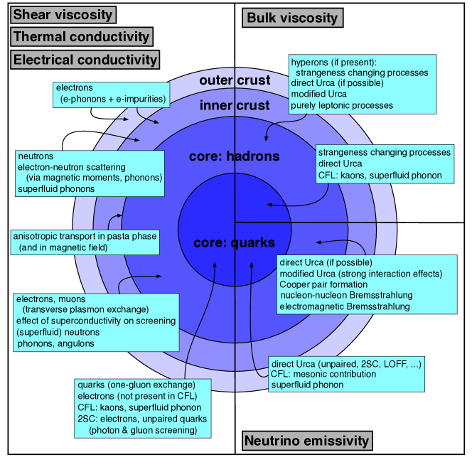
Figure 1: Contributions to the main transport coefficients and to neutrino emission discussed in this review.

I.4 Related reviews

There are a number of reviews that (partially) deal with transport properties in neutron stars, having some overlap with our work, and which we recommend for further reading. Page and Reddy (2012) review transport in the inner crust of the star. A more exhaustive overview of the crust is given by Chamel and Haensel (2008), discussing transport as well as details of the structure and connections to observations. Potekhin et al. (2015) review cooling of isolated neutron stars and discuss transport and thermodynamic properties that are needed to understand the cooling process, including the effect of strong magnetic fields. Cooling in proto-neutron stars just after a core collapse supernova explosion has recently been reviewed by Roberts and Reddy (2017). Many of the currently used results for neutrino emissivity in hadronic matter, including superfluid phases, can already be found in the review by Yakovlev et al. (2001). Superfluidity in neutron stars and some of its effects on transport and reaction rates are reviewed by Page et al. (2014). For a detailed discussion of many-body techniques for hadronic matter inside neutron stars, including neutrino emission processes, see the review by Sedrakian (2007). Transport properties of quark matter are discussed in chapter VII of the review about color superconductivity by Alford et al. (2008a), for a pedagogical discussion of neutrino emissivity in quark matter see Ref. Schmitt (2010). Our review serves as an update to some of these earlier reviews and has a somewhat different focus than most of them, bringing together theoretical results for transport properties from the crust through nuclear matter in the core up to ultra-dense deconfined quark matter.

There are several aspects of transport and reaction rates in neutron stars which we do not discuss or only touch very briefly: we will not elaborate on reactions relevant for neutrino transport in supernovae Burrows et al. (2006) and neutrino-nucleus reactions relevant for supernovae nucleosynthesis Balasi et al. (2015). Nuclear astrophysics in a broader context is discussed by Wiescher et al. (2012) and Schatz (2016), and we refer the reader to the review Meisel et al. (2018) and more specific literature regarding nuclear reactions in accreting crusts Yakovlev et al. (2006); Gupta et al. (2007, 2008); Haensel and Zdunik (2008); Steiner (2012); Afanasjev et al. (2012); Schatz et al. (2014). Neutrino emission reactions in the crust are summarized by Yakovlev et al. (2001) with more recent updates by Chamel and Haensel (2008) and Potekhin et al. (2015), and we have nothing to add to these reviews. Finally, we will not discuss transport in the outer layers of the star, including the atmosphere and the heat blanketing envelopes, where radiative transfer, transport of non-degenerate electrons Potekhin et al. (2015, 2015), and diffusion processes Beznogov and Yakovlev (2013); Beznogov et al. (2016), among others, are important.

II Basic concepts of transport theory

II.1 Basic equations and transport coefficients

We start with a brief introduction to the basic concepts that will be used throughout this review. The goal of this section is to provide the definition of the most important transport coefficients, to show how they appear in the hydrodynamical framework and how they are computed from kinetic theory. In the present section, we shall present a general setup for a dilute gas of one non-relativistic fermionic species. Further assumptions and specifications will be made in the subsequent sections. Our starting point is the Boltzmann equation for the non-equilibrium fermionic distribution function $f({\bm{x}},{\bm{p}},t)$,

$$\frac{\partial f}{\partial t}+\bm{u}\cdot\frac{\partial f}{\partial{\bm{x}}}+{\bm{R}}\cdot\frac{\partial f}{\partial{\bm{p}}}=I[f]\,,$$ (1)

where the particle velocity ${\bm{u}}$ is related to momentum via ${\bm{p}}=m{\bm{u}}$ with the particle mass $m$, and ${\bm{R}}$ is the external force which we do not specify for now, except for assuming that $\nabla_{\bm{p}}\cdot{\bm{R}}=0$. For instance, it can include the gravitational force or, if the particles carry electric charge, the Lorentz force. The collision term is

$$I[f]=-\int_{{\bm{p}}_{1}}\int_{{\bm{p}}^{\prime}}\int_{{\bm{p}}_{1}^{\prime}}W({\bm{p}},{\bm{p}}_{1};{\bm{p}}^{\prime},{\bm{p}}^{\prime}_{1})[ff_{1}(1-f^{\prime})(1-f^{\prime}_{1})-(1-f)(1-f_{1})f^{\prime}f^{\prime}_{1}]\,,$$ (2)

with the the abbreviations $f_{1}=f({\bm{x}}_{1},{\bm{p}}_{1},t)$, $f^{\prime}=f({\bm{x}}^{\prime},{\bm{p}}^{\prime},t)$, $f^{\prime}_{1}=f({\bm{x}}^{\prime}_{1},{\bm{p}}^{\prime}_{1},t)$, and

$$\int_{\bm{p}}\equiv\int\frac{d^{3}{\bm{p}}}{(2\pi\hbar)^{3}}\,.$$ (3)

The collision integral gives the number of collisions per unit time in which a particle with a given momentum ${\bm{p}}$ is lost in a scattering process with another ingoing particle with momentum ${\bm{p}}_{1}$ to produce two outgoing particles with momenta ${\bm{p}}^{\prime}$ and ${\bm{p}}^{\prime}_{1}$, plus the number of collisions of the inverse process, in which a particle with momentum ${\bm{p}}$ is created. The transition rates $W({\bm{p}},{\bm{p}}_{1};{\bm{p}}^{\prime},{\bm{p}}^{\prime}_{1})$ depend on the details of the collision process and contain energy and momentum conservation of the process. Their specific form is not needed for now; we shall see later how the Boltzmann equation is solved approximately in specific cases. For notational convenience, we have omitted the spin variable. One may think of the momentum to actually be a pair of momentum and spin and the momentum integral to include the sum over spin. We have written the collision term in the simplified form that only contains scattering of a given, single particle species with itself. Later, we shall discuss approximate solutions to the Boltzmann equation for more than one particle species, for instance electrons and ions in the neutron star crust.

The Boltzmann equation allows us to derive an equation for the transport of any dynamical variable $\psi(\bm{x},\bm{p},t)$. To this end, we introduce the average value of $\psi$ per particle as

$$\langle\psi\rangle=\frac{1}{n}\int_{\bm{p}}\psi f\,,\qquad n=\int_{\bm{p}}f\,,$$ (4)

where $n$ is the number density. Multiplying the Boltzmann equation with $\psi$ and integrating over momentum then yields

$$\frac{\partial n\langle\psi\rangle}{\partial t}+\nabla\cdot(n\langle\psi\bm{u}\rangle)=n\left(\left\langle\frac{\partial\psi}{\partial t}\right\rangle+\langle\bm{u}\cdot\nabla\psi\rangle+\left\langle\bm{R}\cdot\frac{\partial\psi}{\partial\bm{p}}\right\rangle\right)+\int_{\bm{p}}\psi I[f]\,,$$ (5)

where $\nabla$ is the spatial gradient. The first two terms in the parentheses on the right-hand side account for the production of $\psi$ due to its space and time variations, the third term gives the supply from forces, and the last term gives the production rate from collisions.

From the transport equation (5) we derive the hydrodynamic equations by choosing $\psi$ to be a quantity that is conserved in a collision, such that the momentum integral over $\psi$ times the collision term vanishes. These invariants are $\psi=1$, which corresponds to particle number conservation, energy $\psi=p^{2}/(2m)$, and momentum components $\psi=p_{i}$. Thus we obtain three equations (two scalar equations, one vector equation) that do not depend on the collision term explicitly (but contain the non-equilibrium distribution function, which in principle has to be determined from the full Boltzmann equation). These equations can be written as

$$\frac{\partial\rho}{\partial t}+\nabla\cdot{\bm{g}} = 0\,,$$ (6a)

$$\frac{\partial{\cal E}}{\partial t}+\nabla\cdot{\bm{j}}_{\cal E} = n\bm{R}\cdot\bm{v},$$ (6b)

$$\frac{\partial g_{i}}{\partial t}+\partial_{j}(\Pi_{ji}+\pi_{ji}) = nR_{i}\,.$$ (6c)

Here we have introduced the center-of-mass velocity ${\bm{v}}$. In the present case of a single fluid, this velocity is identical to the drift velocity of the (single) fluid $\langle{\bm{u}}\rangle$. For multi-fluid mixtures, there is a drift velocity for each fluid, which of course does not have to be identical to the total velocity ${\bm{v}}$ of the mixture. This case will become important in the next section, where we discuss electrons in an ion background with a nonzero ${\bm{\vartheta}}\equiv\langle{\bm{u}}\rangle-{\bm{v}}$. In Eq. (6) we have also introduced mass density $\rho=mn$, momentum density ${\bm{g}}=\rho{\bm{v}}$, energy density ${\cal E}={\cal E}_{0}+\rho v^{2}/2$, and stress tensor $\Pi_{ij}=\rho v_{i}v_{j}+\delta_{ij}P$, where the energy density in the co-moving frame of the fluid ${\cal E}_{0}$ and the pressure $P$ are given by

$${\cal E}_{0}=n\langle\varepsilon\rangle=\frac{\rho}{2}\langle w^{2}\rangle\,,\qquad P=\frac{\rho}{3}\langle w^{2}\rangle=\frac{2}{3}{\cal E}_{0}\,,$$ (7)

where ${\bm{w}}\equiv{\bm{u}}-{\bm{v}}$ is the difference between the single-particle velocity and the macroscopic center-of-mass velocity, and

$$\varepsilon=\frac{mw^{2}}{2}$$ (8)

is the single-particle energy in the co-moving frame of the fluid. The flux terms in the energy conservation (6b) and momentum conservation (6c) equations are

$$j_{{\cal E},i}=({\cal E}+P)v_{i}+\pi_{ij}v_{j}+j_{T,i} = \frac{m}{2}\int_{\bm{p}}u^{2}u_{i}f\,,$$ (9a)

$$\Pi_{ij}+\pi_{ij} = m\int_{\bm{p}}u_{i}u_{j}f\,,$$ (9b)

which include the dissipative contributions, which vanish in equilibrium,

$${\bm{j}}_{T}\equiv n\langle\varepsilon\bm{w}\rangle\,,\qquad\pi_{ij}\equiv\rho\langle w_{i}w_{j}\rangle-\delta_{ij}P\,.$$ (10)

We assume that close to equilibrium we can apply the thermodynamic relations ${\cal E}_{0}+P=\mu n+Ts$ and $d{\cal E}_{0}=\mu dn+Tds$ locally, with the $t$ and $\bm{x}$ dependent chemical potential $\mu$, entropy density $s$, and temperature $T$. Using these relations, together with Eqs. (6a) and (6c), the energy conservation (6b) can be written as an equation for entropy production. And, using Eq. (6a), the momentum conservation (6c) can be written in the form of the Navier-Stokes equation. Hence, Eqs. (6b) and (6c) become

$$\frac{\partial s}{\partial t}+\nabla\cdot\left(s{\bm{v}}+\frac{\bm{j}_{T}}{T}\right) = -\frac{\pi_{ji}\partial_{j}v_{i}+{\bm{j}}_{T}\cdot\nabla T/T}{T}\equiv\varsigma\,,$$ (11a)

$$\frac{\partial v_{i}}{\partial t}+({\bm{v}}\cdot\nabla)v_{i} = -\frac{\partial_{i}P}{\rho}+\frac{R_{i}}{m}-\frac{\partial_{j}\pi_{ji}}{\rho}\,,$$ (11b)

where we have defined the entropy production rate $\varsigma$. Instead of deriving the hydrodynamical equations from the Boltzmann equation, we can also view them as an effective theory where dissipative terms can be added systematically with certain transport coefficients. These transport coefficients are then an input to hydrodynamics, for instance computed from a kinetic approach. From Eq. (11a) we see that the dissipative part is composed of products of the thermodynamic forces $\nabla T/T$ and $\partial_{i}v_{j}$ and the corresponding thermodynamic fluxes $\bm{j}_{T}$ and $\pi_{ij}$. The usual transport coefficients are then introduced by assuming linear relations between them with the coefficients being thermal conductivity $\kappa$, shear viscosity $\eta$, and bulk viscosity $\zeta$,

$${\bm{j}}_{T} = -\kappa\nabla T,$$ (12a)

$$\pi_{ij} = -2\eta\left(v_{ij}-\frac{\delta_{ij}}{3}\nabla\cdot{\bm{v}}\right)-\zeta\delta_{ij}\nabla\cdot{\bm{v}}\,,$$ (12b)

where we have abbreviated

$$v_{ij}\equiv\frac{\partial_{i}v_{j}+\partial_{j}v_{i}}{2}\,.$$ (13)

In principle, one can systematically expand the fluxes in powers of derivatives and thus create terms beyond linear order Burnett (1935, 1936); García-Colín et al. (2008). Higher-order hydrodynamical coefficients are rarely used in the non-relativistic context (see however Refs. Chao and Schäfer (2012); Schäfer (2014) for a discussion of second-order hydrodynamics, motivated by applications to unitary Fermi gases). In contrast, second-order relativistic hydrodynamics has been studied much more extensively, motivated by the acausality of the first-order equations and by applications to relativistic heavy-ion collisions Israel and Stewart (1979); Romatschke (2010); Denicol et al. (2012). Here we will not go beyond first order.

The simple one-component monatomic gas discussed above does not have a bulk viscosity $\zeta$ because $\zeta$ is proportional to the trace of $\pi_{ij}$, as we see from Eq. (12b), and the trace of $\pi_{ij}$ vanishes in our simple example, as Eq. (10) shows, due to the relation between energy density and pressure in Eq. (7). In more general cases, the hydrostatic pressure is not given by (7), and the bulk viscosity is nonzero. Notice that the three terms in Eqs. (12) have different spatial symmetry and do not couple. We can compute the rate of the total entropy change $\dot{S}$ of the system by integrating Eq. (11a) over the volume $V$ of the system. Making use of Eqs. (12), we obtain

$$\dot{S} = \int_{V}\frac{d^{3}{\bm{x}}}{T}\left[2\eta\left(v_{ij}-\frac{\delta_{ij}}{3}\nabla\cdot{\bm{v}}\right)^{2}+\zeta(\nabla\cdot{\bm{v}})^{2}+\frac{\kappa(\nabla T)^{2}}{T}\right]-\int_{\partial V}d\bm{\sigma}\cdot\frac{\bm{j}_{T}}{T}\,.$$ (14)

The first integral gives the total entropy production by the dissipative processes inside the system, while the surface integral corresponds to the heat exchange with the external thermostat. Due to the second law of thermodynamics, all phenomenological coefficients $\kappa$, $\eta$, and $\zeta$ have to be non-negative.

In more general cases, the entropy production equation (11a) contains more terms, for instance related to diffusion in multi-component mixtures. Some of these terms will be discussed in the following sections. When additional dissipative processes are considered, the equations become more cumbersome, but the principal scheme is the same.

II.2 Calculating transport coefficients in the Chapman-Enskog approach

Kinetic theory allows us to compute the transport coefficients on microscopic grounds. The basic idea is to expand the distribution function around the local equilibrium distribution function. The kinetic equation then describes the evolution of the system towards local equilibrium. There exist two elaborate methods for this expansion, namely Grad’s moment method Grad (1949) and the Chapman-Enskog method Chapman et al. (1999), see also the textbooks by Kremer (2010) and Zhdanov (2002) for extensive discussions of both methods. Here we give a brief sketch of the Chapman-Enskog method. We write the distribution function as

$$f({\bm{x}},{\bm{u}},t)\approx f^{(0)}+\delta f\,,\qquad\delta f=-\frac{\partial f^{(0)}}{\partial\varepsilon}\Phi+{\cal O}(\Phi^{2})\approx\frac{f^{(0)}(1-f^{(0)})}{k_{B}T}\Phi\,,$$ (15)

with a small correction $\Phi({\bm{x}},t)$ to the Fermi-Dirac function in local equilibrium

$$f^{(0)}({\bm{x}},{\bm{u}},t)=\left\{\exp\left[\frac{\varepsilon({\bm{x}},{\bm{u}},t)-\mu({\bm{x}},t)}{k_{B}T(\bm{x},t)}\right]+1\right\}^{-1}\,,$$ (16)

where $k_{B}$ is the Boltzmann constant and where $\varepsilon$ from Eq. (8) is a function of ${\bm{w}}({\bm{x}},{\bm{u}},t)={\bm{u}}-{\bm{v}}({\bm{x}},t)$. The idea of the following approximation is to only keep the lowest order in $\Phi$ and also drop higher-order terms in the derivatives of $T$, $\mu$, and ${\bm{v}}$. Inserting the ansatz (15) into the Boltzmann equation (1) yields the following lowest order equation

$$\frac{\partial f^{(0)}}{\partial t}+{\bm{u}}\cdot\frac{\partial f^{(0)}}{\partial{\bm{x}}}+{\bm{R}}\cdot\frac{\partial f^{(0)}}{\partial{\bm{p}}}\approx I_{\rm lin}[\Phi]\,,$$ (17)

where $I_{\rm lin}[\Phi]$ is the linearized collision term. To be more general than in the previous section we do not specify its expression for now. [Linearizing the collision term (2) yields Eq. (31).] Note that on the left-hand side the terms proportional to $\Phi$ are counted as higher order since they are multiplied by derivatives of $T$, $\mu$, and ${\bm{v}}$. Certain integral constraints on the deviation functions $\Phi$ can be obtained from the condition that number density, momentum, and energy in a gas volume element must be the same if calculated with the local equilibrium distribution (16) and with the full function $f$ Pitaevskii and Lifshitz (2008).

Let us for now assume the system to be incompressible, which is a good approximation for instance for the neutron star crust. On account of the continuity equation (6a), this is equivalent to $\nabla\cdot{\bm{v}}=0$. (In an incompressible fluid, the density of a fluid element is constant in time, $\partial_{t}\rho+{\bm{v}}\cdot\nabla\rho=0$.) As a consequence, there is no dissipation through bulk viscosity. We shall come back to bulk viscosity later when we address the core of the star. There, bulk viscosity is an important source of dissipation. We also focus on static systems, i.e., we shall neglect all time derivatives. Extending the results of the previous section, we will include the electrical conductivity. To this end, we set ${\bm{R}}=-e{\bm{E}}$, where $\bm{E}$ is the electric field and $e$ is the elementary charge. For now, we do not include a magnetic field and keep the assumption of a single particle species. This assumption deserves a comment. The expression (11a) does not contain the external force $\bm{R}$, indicating that the force does not create dissipation. Of course, the work done by the force $\bm{R}$ affects the energy conservation (6b), but this only enters the bulk motion, as Eq. (11b) shows. Dissipation from the electric field emerges if there exists a friction force which opposes the diffusive motion. This is not described by the collision integral (2), but is realized in a multi-component system such as the electron-ion plasma in the neutron star crust or nuclear matter in the core made of neutrons, protons, and leptons. In this case, as already mentioned below Eq. (6), the average velocity of the constituents $\langle\bm{u}\rangle$ is different from the center-of-mass velocity $\bm{v}$ of the mixture. This gives rise to an electric (and diffusive) current $\bm{j}=-en\bm{\vartheta}=-en(\langle\bm{u}\rangle-\bm{v})$. In the neutron star crust (liquid or solid), due to the small mass ratio $m_{e}/m_{\rm i}$ of electron and ion masses, the contribution of the ion diffusion to the electric current can be neglected. Therefore, the rest frame of the ions is, to a good approximation, identical to the center-of mass frame and we can keep working with a single particle species (the electrons).

With these assumptions, we find for the left-hand side of Eq. (17),

$${\bm{u}}\cdot\frac{\partial f^{(0)}}{\partial{\bm{x}}}-e{\bm{E}}\cdot\frac{\partial f^{(0)}}{\partial{\bm{p}}}=-\frac{\partial f^{(0)}}{\partial\varepsilon}\left[\frac{\varepsilon-h}{T}{\bm{w}}\cdot\nabla T+e{\bm{w}}\cdot{\bm{E}}^{*}+p_{i}w_{j}\left(v_{ij}-\frac{\delta_{ij}}{3}\nabla\cdot{\bm{v}}\right)\right]\,.$$ (18)

Here we work in the co-moving frame of the total fluid, i.e., we have set ${\bm{v}}=0$ after taking the derivatives, such that from now on we have ${\bm{w}}={\bm{u}}={\bm{p}}/m$. We have added a term proportional to $\nabla\cdot{\bm{v}}$ (which is zero in our approximation) in order to reproduce the structure needed for the shear viscosity, defined the enthalpy per particle $h=\mu+sT/n$, and the effective electric field

$${\bm{E}}^{*}={\bm{E}}+\frac{\nabla\mu}{e}+\frac{s}{n}\frac{\nabla T}{e}\,.$$ (19)

The enthalpy is included in the thermal conduction term (proportional to $\nabla T$) to eliminate the convective heat flux [cf. first term in Eq. (9a)].

In order to express the dissipative currents in terms of the deviation function $\Phi$, we re-derive the entropy production equation (11a) as follows. We assume the entropy density of the system close to equilibrium to be given by the usual statistical expression

$$s=-k_{B}\int_{\bm{p}}\left[f\ln f+(1-f)\ln(1-f)\right].$$ (20)

This suggests to set $\psi=\ln f+(f^{-1}-1)\ln(1-f)$ in the general transport equation (5). The right-hand side of that equation, including the collision term as well as the terms from the explicit $({\bm{x}},{\bm{p}},t)$-dependence of $\psi$, yields the entropy production

$$T\varsigma = k_{B}\int_{\bm{p}}[\ln f-\ln(1-f)]\,I[f]=-\int_{\bm{p}}\,\Phi I[f]=\bm{j}\cdot{\bm{E}}^{*}-{\bm{j}}_{T}\cdot\frac{\nabla T}{T}-\pi_{ij}\partial_{j}v_{i}\,.$$ (21)

In the second step we have performed the linearization according to Eq. (15), taking into account that $\varsigma$ vanishes for the local equilibrium function $f^{(0)}$. In the third step, we have used that, according to the Boltzmann equation (17), we can replace the collision integral by Eq. (18), and we have expressed the fluxes in terms of $\Phi$,

$$\bm{j}=e\int_{\bm{p}}\Phi\frac{\partial f^{(0)}}{\partial\varepsilon}{\bm{w}}\,,\qquad\bm{j}_{T}=-\int_{\bm{p}}\Phi\frac{\partial f^{(0)}}{\partial\varepsilon}(\varepsilon-h){\bm{w}}\,,\qquad\pi_{ij}=-\int_{\bm{p}}\Phi\frac{\partial f^{(0)}}{\partial\varepsilon}p_{i}w_{j}\,.$$ (22)

Now, generalizing Eq. (12a), we introduce the transport coefficients associated with the electric and heat fluxes,

$$\left(\begin{array}[]{c}{\bm{E}}^{*}\\[8.61108pt] {\bm{j}}_{T}\end{array}\right)=\left(\begin{array}[]{cc}\frac{1}{\sigma}&-Q_{T}\\[8.61108pt] -Q_{T}T&-\kappa\end{array}\right)\left(\begin{array}[]{c}{\bm{j}}\\[8.61108pt] \nabla T\end{array}\right)\,,$$ (23)

where $\sigma$ is the electrical conductivity and $Q_{T}$ is the thermopower. The form of the non-diagonal terms is a consequence of Onsager’s symmetry principle Pitaevskii and Lifshitz (2008). Notice that due to the same spatial rank-one tensor structure of the thermodynamic forces $\nabla T/T$ and $\bm{E}^{*}$, their linear response laws are coupled. The perturbation that drives the shear viscosity is the second-rank tensor (12b), hence the corresponding response law decouples. In terms of the transport coefficients, the local entropy production rate (21) becomes

$$T\varsigma=\kappa\frac{(\nabla T)^{2}}{T}+\frac{j^{2}}{\sigma}+2\eta\left(v_{ij}-\frac{\delta_{ij}}{3}\nabla\cdot{\bm{v}}\right)^{2}\,,$$ (24)

implying the non-negativeness of $\kappa,\eta,$ and $\sigma$.

The transport coefficients $\eta$, $\kappa$, $\sigma$, $Q_{T}$ can now be computed as follows. To compute the shear viscosity, we make the ansatz

$$\Phi=-A_{\eta}(\varepsilon)\left(p_{i}w_{j}-\frac{\delta_{ij}}{3}\bm{p}\cdot\bm{w}\right)\left(v_{ij}-\frac{\delta_{ij}}{3}\nabla\cdot{\bm{v}}\right)\,,$$ (25)

where, in an isotropic system, the unknown function $A_{\eta}$ only depends on the particle energy. This function has to be determined by inserting the ansatz for $\Phi$ into the linearized Boltzmann equation (17). We can express the shear viscosity through $A_{\eta}$ as

$$\eta=-\frac{2}{15}\int_{\bm{p}}p^{2}w^{2}A_{\eta}(\varepsilon)\frac{\partial f^{(0)}}{\partial\varepsilon}\,.$$ (26)

This relation is obtained by inserting the ansatz (25) into $\pi_{ij}$ from Eq. (22), using the form of the viscous stress tensor (12b) and the angular integral in velocity (or momentum) space (remember that $\bm{p}=m\bm{w}$ in the frame we are working in)

$$\int\frac{d\Omega_{\bm{p}}}{4\pi}w_{i}w_{j}\left(w_{k}w_{\ell}-\frac{\delta_{k\ell}}{3}w^{2}\right)=\frac{w^{4}}{15}\left(\delta_{ik}\delta_{j\ell}+\delta_{i\ell}\delta_{jk}-\frac{2}{3}\delta_{ij}\delta_{k\ell}\right)\,.$$ (27)

In Eq. (26) we have multiplied the result by a factor 2 from the sum over the 2 spin degrees of freedom of a spin-$\frac{1}{2}$ fermion (such that now the integral does not implicitly include the spin sum anymore).

To compute electrical and thermal conductivities and the thermopower, we use the ansatz

$$\Phi=-A_{\kappa}(\varepsilon)\frac{\varepsilon-h}{T}{\bm{w}}\cdot\nabla T-A_{\sigma}(\varepsilon)e\,{\bm{w}}\cdot{\bm{E}}^{*}\,,$$ (28)

with $A_{\kappa}$ and $A_{\sigma}$ computed from the linearized Boltzmann equation, and the transport coefficients are found in an analogous way as just demonstrated for the shear viscosity: we insert the ansatz (28) into ${\bm{j}}$ and ${\bm{j}}_{T}$ from Eq. (22), perform the angular integral,

$$\int\frac{d\Omega_{\bm{p}}}{4\pi}w_{i}w_{j}=\frac{w^{2}\delta_{ij}}{3}\,,$$ (29)

and compare the result with Eq. (23) to obtain (again taking into account the 2 spin degrees of freedom)

$$\sigma = -\frac{2e^{2}}{3}\int_{\bm{p}}w^{2}A_{\sigma}(\varepsilon)\frac{\partial f^{(0)}}{\partial\varepsilon}\,,$$ (30a)

$$\sigma Q_{T} = -\frac{2e}{3}\int_{\bm{p}}w^{2}A_{\kappa,\sigma}(\varepsilon)\frac{\varepsilon-h}{T}\frac{\partial f^{(0)}}{\partial\varepsilon}\,,$$ (30b)

$$\kappa+\sigma Q_{T}^{2}T = -\frac{2}{3}\int_{\bm{p}}w^{2}A_{\kappa}(\varepsilon)\frac{(\varepsilon-h)^{2}}{T}\frac{\partial f^{(0)}}{\partial\varepsilon}\,,$$ (30c)

from which $\sigma$, $Q_{T}$, and $\kappa$ can be computed. As a consequence of Onsager’s symmetry principle, we have obtained two expressions for $\sigma Q_{T}$, using either $A_{\sigma}$ or $A_{\kappa}$ in the integral.

In general, even the solution of the linearized Boltzmann equation is not an easy task and various methods and approximations are used. First, one needs to specify the explicit expression for the collision integral. For instance, the linearization of the collision integral (2) gives

$$I_{\rm lin}[\Phi]=-\frac{1}{k_{B}T}\int_{{\bm{p}}_{1}}\int_{{\bm{p}}^{\prime}}\int_{{\bm{p}}_{1}^{\prime}}W({\bm{p}},{\bm{p}}_{1},{\bm{p}}^{\prime},{\bm{p}}^{\prime}_{1})f^{(0)}f_{1}^{(0)}(1-f^{\prime(0)})(1-f^{\prime(0)}_{1})(\Phi+\Phi_{1}-\Phi^{\prime}-\Phi^{\prime}_{1})\,,$$ (31)

where we have used $f^{(0)}f_{1}^{(0)}(1-f^{\prime(0)})(1-f^{\prime(0)}_{1})=(1-f^{(0)})(1-f_{1}^{(0)})f^{\prime(0)}f^{\prime(0)}_{1}$ due to energy conservation.

One of the simplest cases is realized when the collision integral can be written in the form of the (energy-dependent) relaxation-time approximation,

$$I=-\sum_{lm}\frac{\delta f^{lm}}{\tau^{l}(\varepsilon)}Y_{lm}(\Omega_{\bm{p}})\,,$$ (32)

which takes into account the angular dependence of the deviation to the equilibrium distribution function by expanding it in spherical harmonics $Y_{lm}$. Here $\tau^{l}(\varepsilon)$ is the relaxation time for the perturbation of multiplicity $l$. The solution of the Boltzmann equation is then

$$A_{\sigma}(\varepsilon)=A_{\kappa}(\varepsilon)=\tau^{1}(\varepsilon)\,,\qquad A_{\eta}(\varepsilon)=\tau^{2}(\varepsilon)\,.$$ (33)

When the relaxation time approximation is not available, one usually represents the functions $A(\varepsilon)$ in the form of a series expansion in some basis functions. This basis has to be chosen carefully for a satisfactory convergence of the expansion. In some cases the infinite chain of equations for the coefficients can be solved analytically and the exact solution for the transport coefficients is obtained from (30) (in form of an infinite series). In practice, the chain of equations is truncated at a finite number of coefficients. The truncation procedure is justified on the basis of the variational principle of kinetic theory Ziman (2001). The variational principle uses the fact that the entropy production rate calculated from (21) with the linearized collision integral $I[\Phi]$ is a semi-positive definite functional of $\Phi$. This is readily seen for the binary collision integral (31) since the probability $W$ is positive, but it holds in general. Suppose that the arbitrary function $\tilde{\Phi}$ is subject to the constraint

$$\int_{\bm{p}}X\tilde{\Phi}=\int_{\bm{p}}I_{\rm lin}[\tilde{\Phi}]\tilde{\Phi}=-T\varsigma[\tilde{\Phi}]\,,$$ (34)

where we have abbreviated (18) by $X$. The variational principle states that over the class of such functions, the entropy production is maximal for the solution of the Boltzmann equation $X=I_{\rm lin}[\Phi]$, in other words $\varsigma[\Phi]\geq\varsigma[\tilde{\Phi}]$. Increasing the number of terms in the functional expansion and maximizing the functional $\varsigma[\tilde{\Phi}]$ under the constraint (34), one approaches the exact solution. This principle can be reformulated to give a direct limit on the diagonal coefficients in the Onsager relations. For instance, setting the thermodynamic forces to zero, $\nabla T/T=0$ and $v_{ij}=0$, and keeping only $\bm{E}^{*}$, one obtains the electrical conductivity by minimizing

$$\frac{1}{\sigma}\leq\frac{E^{*2}}{T\varsigma[\tilde{\Phi}]}$$ (35)

over the functions subject to (34). Notice that the off-diagonal coefficient $Q_{T}$ cannot be constrained in this way.

The variational principle discussed here applies for the stationary case in the absence of a magnetic field. The extension of the variational principle beyond this approximation is non-trivial and is outside the scope of the present section.

II.3 Towards neutron star conditions

In this section we briefly comment on some modifications and extensions of the kinetic theory laid out in the previous sections due to the specific conditions inside neutron stars. We mention plasma effects, transport in Fermi liquids, relativistic effects, and effects from Cooper pairing.

II.3.1 Plasma effects

Electrically charged particles, for instance electrons in the crust and in the core, interact via the long-range Coulomb potential. This seems to be at odds with the concept of instant binary collisions, which forms the basis of the Boltzmann approach to compute transport properties of dilute gases. However, the interaction between charged particles in a plasma is screened and thus is effectively damped on length scales $r>r_{D}$, where $r_{D}$ is the Debye screening length. Therefore, the Boltzmann equation becomes appropriate to describe the processes occurring on large scales, provided the screened interaction potential is used in the collision integral Pitaevskii and Lifshitz (2008). The screening itself depends on the distribution functions of the plasma components, which severely complicates the solution. However, for weak deviations from equilibrium, when the linearized Boltzmann equation is used, the screening which enters the collision integral in Eq. (17) can be calculated from the equilibrium distribution functions (i.e., in the collisionless limit). Additional justification comes from the degeneracy conditions, which are appropriate for electrons in most parts of the star (and other charged particles in the core). In this case, only a small fraction of the thermal excitations contribute to transport phenomena. Moreover, the kinetic energy of the particles increases with density stronger than the Coulomb interaction energy. In other words, the denser the gas is, the closer it is to the ideal Fermi gas Landau and Lifshitz (1980). All these properties allow us to use the formalism of the linearized Boltzmann equation discussed above. Note that the force term ${\bm{R}}$ should contain the Lorentz force with the self-consistent electromagnetic field. The generalized Ohm law (23) then is written in the co-moving frame of the plasma and contains the electric field measured in this frame, ${\bm{E}}^{\prime}=\bm{E}+\frac{1}{c}{\bm{v}}\times{\bm{B}}$. We will return to this aspect in more details in Sec. IV.1.5.

The ions in the neutron star crust are non-degenerate and non-ideal. The discussion of their transport phenomena is more involved. Fortunately, the ion contribution is usually negligible, see Sec. III.

II.3.2 Transport in Fermi liquids

Nuclear matter in the core of a neutron star is a strongly interacting, non-ideal, multi-component fluid. The kinetic theory of rarefied gases described above cannot be applied directly. However, the relevant temperatures are low and the matter is highly degenerate. In this case, the framework of Landau’s Fermi-liquid theory Baym and Pethick (1991) can be used to describe the low-energy excitations of the system. The excitations are considered as a dilute gas of quasiparticles which obey the Fermi-Dirac distribution (16) in momentum space, normalized to give the total local number density $n$ of the real particles. The single-quasiparticle energy $\varepsilon(\bm{p})$ is a functional of the distribution function $f$, the quasiparticle Fermi momentum is $p_{F}=\hbar(3\pi^{2}n)^{1/3}$, and in equilibrium the spectrum of quasiparticles in the vicinity of the Fermi surface is described by the effective mass on the Fermi surface $m^{*}=p_{F}/v_{F}$, where

$$\varepsilon^{(0)}-\mu=v_{F}(p-p_{F})\,,\qquad v_{F}=\left(\frac{\partial\varepsilon^{(0)}}{\partial p}\right)_{p=p_{F}},$$ (36)

with the Fermi velocity $v_{F}$, and the superscript $(0)$ indicates equilibrium.

The evolution of the quasiparticle distribution function is described by the Landau transport equation

$$\frac{\partial f}{\partial t}+\bm{u}\cdot\frac{\partial f}{\partial{\bm{x}}}-\nabla\varepsilon\cdot\frac{\partial f}{\partial{\bm{p}}}=I[f]\,,$$ (37)

where now $\bm{u}=\nabla_{\bm{p}}\,\varepsilon$. The equation (37) is different from the Boltzmann equation (1) since the term $\nabla\varepsilon$ is present even in the absence of external forces $\bm{R}$. This is because the energy spectrum – being a functional of $f$ – changes from one coordinate point to another. Thus, $\nabla\varepsilon$ contains the combined effects of the external forces and the effective field resulting from interactions between quasiparticles. In addition, the quasiparticle velocity is coordinate-dependent for the same reason.

Transport coefficients of the Fermi-liquid are computed by considering a small deviation from local equilibrium and performing the linearization of the Landau equation in a way similar to Sec. II.2 Baym and Pethick (1991); Pitaevskii and Lifshitz (2008). However, there is an important difference. The local equilibrium distribution function is $f^{(0)}(\varepsilon^{(0)})$, but the conservation laws from the collision integral employ the true quasiparticle energies $\varepsilon$. Hence the collision integral vanishes for the functions $f^{(0)}(\varepsilon)$ instead of true local distribution function. As a consequence, the linearized collision integral depends not on $\delta f=f-f^{(0)}(\varepsilon^{(0)})$ but on $\delta\tilde{f}=f-f^{(0)}(\varepsilon)$, and the definition of the function $\Phi$ (15) is modified to

$$\delta\tilde{f}=-\frac{\partial f^{(0)}}{\partial\varepsilon}\Phi\,.$$ (38)

Since the definitions of the fluxes also contain the true quasiparticle energies and velocities, they are given by the expressions (22) with $\Phi$ redefined according to (38). Therefore, in the stationary case, we obtain formally identical equations as in the above derivation. Fermi-liquid effects do not appear explicitly. The same is true if a magnetic field is taken into account Pitaevskii and Lifshitz (2008). In more general cases, terms containing $\delta f$ can appear on the left-hand side of the linearized Boltzmann equation. This situation is realized for instance when the bulk viscosity of the Fermi liquid is considered Baym and Pethick (1991); Sykes and Brooker (1970).

II.3.3 Relativistic effects

Neutron stars are ultra-dense objects, and thus relativistic effects are important for the transport in the star. They manifest themselves in various forms, and we have to distinguish between effects on a microscopic level (e.g., calculations of transport coefficients) and a macroscopic level (e.g., simulations based on hydrodynamic equations), as well as between effects from special relativity (large velocities) and general relativity (spacetime curvature on scales of interest). In this review, we are almost exclusively concerned with microscopic calculations, where we can usually ignore effects from general relativity. The reason is the large separation of the scale on which the gravitational field changes inside the star from the microscopic scales on which the equilibration processes (collisions or reactions) operate Tauber and Weinberg (1961); Thorne (1966). If the mean free paths of the particles are microscopic in this sense, one can study transport processes in the local Lorentz frame, and gravity effectively does not appear in the analysis. If the mean free path, however, becomes comparable to the macroscopic scale of gravity, one has to consider the full general relativistic transport equation Vereshchagin and Aksenov (2017)

$$p^{\mu}\frac{\partial f}{\partial x^{\mu}}-\Gamma^{\mu}_{\;\;\nu\rho}\,p^{\nu}p^{\rho}\frac{\partial f}{\partial p^{\mu}}=I[f]\,,$$ (39)

where we have omitted external forces, where $\Gamma^{\mu}_{\;\;\nu\rho}$ are the Christoffel symbols, $x^{\mu}$ is the spacetime four-vector, $p^{\mu}$ the four-momentum, and $I[f]$ is the collision integral (specified in the local reference frame). This situation occurs for instance for neutrino transport in supernovae and proto-neutron stars Pons et al. (1999). In neutron stars, this general approach may be important for example in superfluid phases if the only available excitations are the Goldstone modes, whose mean free path can become of the order of the size of the star, see Secs. IV.1.4 and V.5.2. Effects from general relativity are also important when transport coefficients – computed from a microscopic approach – are used as an input for hydrodynamic equations. These equations, when they concern the structure of the whole star or a significant fraction of it, must be formulated within general relativity. An example is the equation for the radial component of the heat flux in a cooling star Thorne (1966, 1977),

$$F_{r}=-\kappa\,e^{-\lambda-\phi}\frac{\partial\tilde{T}}{\partial r}\,,$$ (40)

where $\kappa$ is the thermal conductivity, $\lambda$ and $\phi$ appear in the parametrization of the metric,

$$ds^{2}=e^{2\phi}d(ct)^{2}-e^{2\lambda}dr^{2}-r^{2}(d\theta^{2}+\sin^{2}\theta\,d\varphi^{2})\,,$$ (41)

and $\tilde{T}\equiv Te^{\phi}$ is the redshifted temperature. (It is the redshifted temperature, not the temperature $T$, which is constant in equilibrium.)

To connect the non-relativistic hydrodynamic equations of Sec. II.1 to a covariant formalism, one introduces the (special) relativistic stress-energy tensor,

$$T^{\mu\nu}=T^{\mu\nu}_{\rm ideal}+T^{\mu\nu}_{\rm diss}\,,$$ (42)

where we have separated the ideal part $T^{\mu\nu}_{\rm ideal}$ from the dissipative contribution $T^{\mu\nu}_{\rm diss}$,

$$T^{\mu\nu}_{\rm ideal} = (\epsilon+P)v^{\mu}v^{\nu}-g^{\mu\nu}P\,,$$ (43a)

$$T^{\mu\nu}_{\rm diss} = \kappa(\Delta^{\mu\gamma}v^{\nu}+\Delta^{\nu\gamma}v^{\mu})[\partial_{\gamma}T+T(v\cdot\partial)v_{\gamma}]+\eta\Delta^{\mu\gamma}\Delta^{\nu\delta}\left(\partial_{\delta}v_{\gamma}+\partial_{\gamma}v_{\delta}-\frac{2}{3}g_{\gamma\delta}\partial\cdot v\right)+\zeta\Delta^{\mu\nu}\partial\cdot v\,.$$ (43b)

Here, $\epsilon$ and $P$ are energy density and pressure measured in the rest frame of the fluid, $g^{\mu\nu}=(1,-1,-1,-1)$ is the metric tensor in flat space, $v^{\mu}=\gamma(1,{\bm{v}})$ is the four-velocity with the Lorentz factor $\gamma$ and the three-velocity ${\bm{v}}$ used in Secs. II.1 and II.2. We have abbreviated $\Delta^{\mu\nu}=g^{\mu\nu}-v^{\mu}v^{\nu}$, and the transport coefficients $\kappa$, $\eta$, $\zeta$ are heat conductivity, shear and bulk viscosity, as in the non-relativistic formulation (12). In the non-relativistic limit, using the notation from Sec. II.1, $T^{00}_{\rm ideal}\to{\cal E}$ is the energy density, $T^{0i}_{\rm ideal}\to g_{i}$ is the momentum density, $T^{i0}_{\rm ideal}\to({\cal E}+P)v_{i}$ is the non-dissipative part of the energy flux ${\bm{j}}_{\cal E}$, and $T^{ij}_{\rm ideal}\to\Pi_{ij}$ is the non-relativistic stress tensor. The dissipative terms are formulated in the so-called Eckart frame Eckart (1940), where – in contrast to the Landau frame Landau and Lifshitz (1987) – the conserved four-current $j^{\mu}=nv^{\mu}$ does not receive dissipative corrections Kovtun (2012). The hydrodynamic equations are then obtained from the conservation laws for the stress-energy tensor and the current,

$$\partial_{\mu}T^{\mu\nu}=\partial_{\mu}j^{\mu}=0\,.$$ (44)

They reduce to Eqs. (6) in the non-relativistic limit. We will briefly return to this relativistic formulation in Sec. V.4.2, but otherwise we will not discuss any of the effects illustrated by Eqs. (39), (40), and (43). In particular, since we do not discuss neutrino transport in supernovae, no effects from general relativity will be further discussed. Therefore, when we use ‘relativistic’ in the rest of the review, we mean effects from special relativity in the following simple sense: relativistic effects are important if the rest mass (times the speed of light) of a given particle species is not overwhelmingly larger than its Fermi momentum. (In this case, the Fermi velocity introduced in the previous section, i.e., the slope of the dispersion relation at the Fermi surface, becomes a sizable fraction of the speed of light.) With this criterion, the ions in the crust and the nucleons in the core are often treated non-relativistically (for ultra-high densities in the core, this treatment becomes questionable), while the lighter electrons and quarks are relativistic (except for electrons at very low densities in the outer crust).

II.3.4 Transport with Cooper pairing

The effect of Cooper pairing on reaction rates and transport will be discussed specifically in various sections throughout the review. As a preparation and a simple overview, we now give some general remarks that may be helpful to understand and put into perspective the more detailed discussions and results. For a pedagogical introduction, bringing together elements from non-relativistic and relativistic approaches to Cooper pairing in superfluids and superconductors see Ref. Schmitt (2015).

Cooper pairing in neutron stars is expected to occur in the inner crust for neutrons and in the core for neutrons, protons, and, if present, for hyperons and quarks. The critical temperatures of these systems vary over several orders of magnitude, depending on the form of matter, on density, and on the particular pairing channel. Moreover, it is prone to large uncertainties because the attractive force needed for Cooper pairing originates from the strong interaction. Nevertheless, a rough benchmark to keep in mind is $T_{c}\sim 1\,{\rm MeV}$, which is the maximal critical temperature reached for nuclear matter (with significantly smaller values for neutron triplet pairing) and which is exceeded by about an order of magnitude, maybe even two, by quark matter, where $T_{c}\sim(10-100)\,{\rm MeV}$ (also in quark matter, there are pairing patterns with significantly lower critical temperatures). In any case, we conclude that the temperatures inside the star – except for very young neutron stars – are sufficiently low to allow for Cooper pairing. The resulting stellar superfluids and superconductors Alford et al. (2008a); Page et al. (2014); Haskell and Sedrakian (2017) are similar to their relatives in the laboratory, but the situation in the star is typically more complicated. For instance, the neutron superfluid in the inner crust coexists with a lattice of ions, the core might be a superconductor and a superfluid at the same time, and quark matter might introduce effects of color superconductivity. In addition, the star rotates and has a magnetic field, which suggests the presence of superfluid vortices and possibly magnetic flux tubes, which may coexist and interact with each other. Therefore, understanding superfluid transport in the environment of a neutron star is a difficult task, and some care is required in using results from ordinary superfluids.

One obvious effect of Cooper pairing is the suppression of reaction rates and scattering processes of the fermions that pair. This effect is very easy to understand. Cooper pairing induces an energy gap $\Delta$ in the quasiparticle dispersion relation (one needs a finite amount of energy to break up a pair), and thus, for temperatures much smaller than the gap, quasiparticles are not available for a given process. As a consequence, if at least one of the participating fermions is gapped, the rate is exponentially suppressed by a factor $\exp(-\Delta/T)$ for $T\ll\Delta$. The suppression is milder if the pairing is not isotropic and certain directions in momentum space are left ungapped. This is conceivable for some forms of neutron pairing and in certain color-superconducting quark matter phases. In this case, if for instance only one- or zero-dimensional regions of the Fermi surface contribute (as opposed to the full two-dimensional Fermi surface in the unpaired case), the rate is suppressed by a power of the small parameter $T/\Delta$. Except for these special cases, at low temperatures we can usually neglect the processes suppressed by Cooper pairing and can restrict ourselves to contributions from ungapped fermions or other low-energy excitations, if present.

At larger temperatures, as we move towards the critical temperature $T_{c}$, the form of the exponential suppression no longer holds and the rate in the Cooper-paired phase has to be evaluated numerically. Since particle number conservation is broken spontaneously, particles can be deposited into or created from the Cooper pair condensate. This effect induces subprocesses that are called Cooper pair breaking and formation processes. They are particularly interesting in nuclear matter, where more efficient processes, such as the direct Urca process, are suppressed. Then, somewhat counterintuitively, an enhancement of the neutrino emission is possible as the system cools through the critical temperature for neutron superfluidity.

While Cooper pairing removes fermionic degrees of freedom from transport at low temperatures, it introduces one or several massless bosonic excitations if a global symmetry is spontaneously broken by the formation of a Cooper pair condensate. This is due to the Goldstone theorem, and the corresponding Goldstone mode for superfluidity is, following the terminology of superfluid helium, usually called phonon (or ‘superfluid mode’, or ‘superfluid phonon’ to distinguish it from the lattice phonons in the neutron star crust). In this case, the broken global symmetry is the $U(1)$ associated with particle number conservation. Superfluid neutron matter and the color-flavor locked (CFL) quark matter phase both have a phonon. Transport through phonons is mostly computed with the help of an effective theory, and we will quote some of the resulting transport properties in hadronic and quark matter. If Cooper pairing breaks additional global symmetries, such as rotational symmetry, additional Goldstone modes appear. This is possible in ${}^{3}P_{2}$ neutron pairing Bedaque and Nicholson (2013); Bedaque and Reddy (2014) and in spin-one color superconductivity Pang et al. (2011).

If instead a local symmetry is spontaneously broken, there is no Goldstone mode. This is the case for Cooper pairing of protons and for quark matter phases other than CFL such as the so-called 2SC phase (although, due to the presence of electrons and the resulting screening effects, the Goldstone mode in a proton superconductor can be ‘resurrected’ Baldo and Ducoin (2011)). As in ordinary superconductivity, the would-be Goldstone boson is replaced by an additional degree of freedom of the gauge field, which acquires a magnetic mass. One obvious consequence is the well-known Meissner effect, which is of relevance for the magnetic field evolution in neutron stars. Magnetic screening can also indirectly affect transport properties if a certain transport property is dominated by one (unpaired) particle species that is charged under the gauge symmetry which is spontaneously broken by Cooper pairing of a different species (even though the species that pairs does not contribute to transport itself because it is gapped). This situation occurs in nuclear matter when electrons experience a modified electromagnetic interaction due to pairing of protons, and in the 2SC phase of quark matter, where the different particle species are electrons and the different colors and flavors of quarks, which are not all paired in this specific phase, and the relevant gauge bosons are the gluons and the photon.

As we know from some of the earliest experiments with superfluid helium, a superfluid at nonzero temperature (below $T_{c}$) behaves as a two-fluid system Tisza (1938); Landau (1941) (for the connection of the two-fluid picture to an underlying microscopic theory see for instance Ref. Alford et al. (2013)). This means that, in a hydrodynamic approach, there are two independent velocity fields: one for the superfluid component, which is the Cooper pair condensate in a fermionic superfluid (or the Bose-Einstein condensate in a bosonic superfluid such as ⁴He), and one for the so-called normal component, which corresponds to the phonons and possibly a fraction of the fermions which have remained unpaired. Since only the normal component carries entropy, the two-fluid nature has obvious consequences for heat transport, which now can occur through a counterflow of the two fluid components. While this mechanism proves extremely efficient in laboratory experiments with superfluid helium, it may be less effective in the more complicated situation in a neutron star. For instance, in the inner crust of the star the counterflow of the normal and superfluid components becomes dissipative due to the presence of electrons which damp the motion of the normal fluid through induced electron-phonon interactions Page and Reddy (2012). Another consequence of the two-fluid behavior is the existence of second sound. (The phonon, first and second sound are in general three different excitations. At low temperatures, the phonon excitation is identical to first sound, while close to the critical temperature it is identical to second sound Alford et al. (2014a).) In superfluid helium, first and second sound are predominantly density and temperature oscillations, respectively, for all temperatures $T<T_{c}$. This is not necessarily true for other superfluids and it has been shown that first and second sound may exchange their roles Alford et al. (2014a).

Two-fluid systems allow for additional transport coefficients. For instance, in the hydrodynamics of a superfluid, usually three independent bulk viscosity coefficients are taken into account Khalatnikov (1965). In a neutron star, the situation might become even more complicated due to the presence of additional fluid components, e.g., a nonzero-temperature neutron superfluid coexisting with electrons and protons, such that we have to deal with an involved multi-fluid system. One interesting feature of multi-fluids with relevance for the physics of neutron stars is the possibility of hydrodynamical instabilities due to a counterflow between the fluids. Such an instability may occur for the neutron superfluid in the inner crust, if it moves (locally) with a sufficiently large nonzero velocity relative to the ion lattice. In this review, we shall not further discuss multi-fluid transport in detail (except for the transport coefficients of a single superfluid at nonzero $T$) and refer the reader to the recent literature and references therein Gusakov et al. (2009a, b); Glampedakis et al. (2012a); Chamel (2013); Andersson et al. (2013); Haber et al. (2016); Andersson et al. (2017).

Finally, let us mention another very important consequence of Cooper pairing, which has been related to various astrophysical observations such as pulsar glitches Haskell and Melatos (2015), namely the formation of rotational vortices in a superfluid and of magnetic flux tubes in a superconductor. (A magnetic field enters a type-II superconductor through quantized magnetic flux tubes if its magnitude lies between the upper and lower critical magnetic fields. The presence of a superfluid, to which the superconductor couples, may change the textbook-like behavior of type-II superconductors qualitatively Haber and Schmitt (2017a, b).) Besides ordinary vortices in hadronic matter, quark matter in the core of neutron stars may contain so-called semi-superfluid vortices Balachandran et al. (2006); Alford et al. (2016) in the CFL phase and/or color magnetic flux tubes Alford and Sedrakian (2010); Glampedakis et al. (2012b) in the CFL or 2SC phases (the latter are not protected by topological arguments and it is unknown if they are energetically stable objects in the neutron star environment). As for most of the multi-fluid aspects, we will not review the transport properties of superfluids in the presence of vortices. For various aspects of the hydrodynamics of these systems, including the possibility of superfluid turbulence and possible boundaries between phases with and without (or with a different kind of) vortices, see Refs. Hall and Vinen (1956); Khalatnikov (1965); Donnelly (1999); Gusakov (2016); Gusakov and Dommes (2016); Graber et al. (2017).

III Transport in the crust and the crust/core transition region

III.1 Thermal and electrical conductivity and shear viscosity

The main carriers which determine the transport processes in the neutron star crust are electrons. The electrons in the crust form an almost ideal, degenerate gas. The degeneracy temperature $T_{F}$ for electrons is

$$T_{Fe}=\frac{\mu_{e}-m_{e}c^{2}}{k_{B}}=5.9\times 10^{9}{\rm K}\left(\sqrt{1+x_{r}^{2}}-1\right)\,,$$ (45)

where $x_{r}=p_{Fe}/(m_{e}c)$ is the electron relativistic parameter, with the electron Fermi momentum $p_{Fe}$, the electron rest mass $m_{e}$, and the electron chemical potential (including the rest mass) $\mu_{e}=m_{e}c^{2}\sqrt{1+x_{r}^{2}}\equiv m_{e}^{*}c^{2}$. In a one-component plasma with ion charge number $Z$ and total nucleon number per ion $A$, $x_{r}\approx(\rho_{6}Z/A)^{1/3}$, where $\rho_{6}$ is the mass density $\rho$ in units of $10^{6}\,{\rm g}\,\rm{cm}^{-3}$. In most of the crust, $\rho_{6}\gg 1$ and the electrons are ultra-relativistic. We will not discuss electrons in non-degenerate or partially degenerate conditions $T\gtrsim T_{Fe}$. The effects of non-degenerate electrons are important when the thermal structure of the stellar heat blanket is calculated. In non-degenerate regions the radiative contribution to heat transport is relevant, which we also do not discuss here, for details see Refs. Potekhin et al. (2015, 2015).

For degenerate electrons ($T\ll T_{Fe}$) the analysis of the Boltzmann equation is simplified since the transport is mainly provided by those electrons whose energies lie in a narrow thermal band near the Fermi surface $|\varepsilon-\mu_{e}|\lesssim k_{B}T$. When using Eqs. (25) and (30), it is safe to set $h=\mu_{e}$ and neglect the thermopower correction in Eq. (30c). As a result, it is convenient to present the transport coefficients of interest in the form

$$\sigma = \frac{e^{2}n_{e}\tau_{\sigma}}{m_{e}^{*}}\,,$$ (46a)

$$\kappa = \frac{\pi^{2}k_{B}^{2}Tn_{e}\tau_{\kappa}}{3m_{e}^{*}}\,,$$ (46b)

$$Q_{T} = \frac{\pi^{2}k_{B}^{2}Tm_{e}^{*}}{3ep^{2}_{Fe}}(3+\xi)\,,$$ (46c)

$$\eta = \frac{n_{e}p^{2}_{Fe}\tau_{\eta}}{5m_{e}^{*}}\,,$$ (46d)

where $\tau_{\sigma}$, $\tau_{\kappa}$, and $\tau_{\eta}$ are the effective relaxation times, and $\xi\sim 1$ is a dimensionless factor which can change sign depending on the electron scattering mechanism. For brevity, we will not consider the thermopower coefficient further. The inverse quantities $\nu_{\sigma,\kappa,\eta}=\tau^{-1}_{\sigma,\kappa,\eta}$ are called the effective collision frequencies. If the relaxation time approximation (32) is applicable, the effective relaxation times become the actual relaxation times evaluated at the Fermi surface, $\tau_{\sigma}=\tau_{\kappa}=\tau^{1}_{e}(\mu_{e})$, $\tau_{\eta}=\tau^{2}_{e}(\mu_{e})$, cf. Eq. (33), since one approximates $\frac{\partial f^{(0)}}{\partial\varepsilon}\approx-\delta(\varepsilon-\mu_{e})$. In this case, we obtain the standard Wiedemann-Franz rule for conductivities,

$$\frac{\kappa}{\sigma}=\frac{\pi^{2}k_{B}^{2}T}{3e^{2}}.$$ (47)

The relaxation time approximation holds when electron-ion collisions are the dominant scattering mechanism and the energy $\omega$ transferred in these collision is small $\omega\ll k_{B}T$. When this is not the case, the variational calculations outlined in Sec. II.2 are usually employed. It turns out that already the simplest variational approximation gives a satisfactory estimate for astrophysical conditions. Moreover, the violation of the Wiedemann-Franz rule is not as dramatic as in ordinary metals at low temperature Yakovlev and Urpin (1980).

When there are different relaxation mechanisms for the electron distribution function, for instance collisions with different particle species, the respective collision integrals must be added on the right-hand side of the Boltzmann equation. In practice, one usually considers different mechanisms separately to obtain the effective collision frequency $\nu_{ej}$ for each scattering process. Due to the strong degeneracy of electrons, the cumulated collision frequency $\nu_{\rm tot}=\sum_{j}\nu_{ej}$ obtained in this way is a good approximation to the solution of the Boltzmann equation with all mechanisms included. This is known as Matthiessen’s rule Ziman (2001). The variational principle of kinetic theory allows us to estimate the error introduced by this approximation Ziman (2001), see also Ref. Potekhin et al. (2015). Below we consider the most important processes that determine the electron transport.

III.1.1 Electron-ion collisions

The main process for electron transport is their scattering off ions. The ions in the neutron star crust form a strongly coupled non-ideal plasma, whose state is defined by an ion coupling parameter $\Gamma$. For a one-component plasma (in the sense that only one sort of ions is present)

$$\Gamma=\frac{Z^{2}e^{2}}{a_{\rm WZ}k_{B}T}\approx 153\,x_{r}\left(\frac{Z}{50}\right)^{5/3}\left(\frac{T}{10^{8}\leavevmode\nobreak\ {\rm K}}\right)^{-1}\,,$$ (48)

where the ion Wigner-Seitz cell radius $a_{\rm WZ}$ is defined by the relation

$$\frac{4\pi}{3}a_{\rm WZ}^{3}n_{\rm i}=1\,.$$ (49)

When $\Gamma\ll 1$, ions are in the gaseous phase, at $\Gamma\gtrsim 1$ in the liquid phase, and at $\Gamma=\Gamma_{\rm m}\approx 175$ Potekhin and Chabrier (2000) the ion liquid crystallizes and is thought to form a body-centered cubic lattice Chamel and Haensel (2008). This condition and Eq. (48) define the (density-dependent) melting temperature $T_{\rm m}$. Notice that the melting point can shift substantially if the electron polarization or magnetic field effects are taken into account Potekhin and Chabrier (2000); Potekhin and Chabrier (2013). Another important parameter is the ion plasma temperature

$$T_{\rm pi}=\frac{\hbar}{k_{B}}\left(\frac{4\pi Z^{2}e^{2}n_{\rm i}}{m_{\rm i}}\right)^{1/2},$$ (50)

above which the thermodynamic properties are classical, and below which quantum effects should be taken into account. In the context of electron transport, the important point is that at $T<T_{\rm pi}$ the typical energy transferred in the electron-ion collisions is $\omega\sim k_{B}T$ and the relaxation time approximation cannot be used Yakovlev and Urpin (1980). If $T_{\rm pi}<T_{\rm m}$, quantum effects are only important in the crystalline phase. A temperature regime where quantum effects are relevant in the liquid phase can in principle be realized for light elements and high densities. In this case, the properties of the liquid – including transport properties – are modified, but also the crystallization point itself (the value $\Gamma_{\rm m}\approx 175$ is obtained from a classical estimate, not taking into account zero-point vibrations). Calculations show that at some density the crystallization temperature starts to decrease and reaches zero at a certain critical density, above which no crystallization occurs Chabrier (1993); Jones and Ceperley (1996). However, the importance of a quantum liquid regime for neutron star envelopes is questionable since nuclear reactions (electron captures and pycno-nuclear burning) would not allow light elements to exist at sufficiently large densities, see Sec. 2.3.5 of Ref. Haensel et al. (2007) for more details. Therefore, here we discuss quantum corrections only for the solid phase (see footnote 4 for a brief remark about results for the quantum liquid regime).

For any phase state of the ions, the effective electron-ion collision frequency, to be used in (46), is usually written in terms of the effective Coulomb logarithm $\Lambda_{e{\rm i}}$,

$$\nu_{e{\rm i}}=\frac{4\pi Z^{2}e^{4}n_{\rm i}}{p_{Fe}^{2}v_{Fe}}\Lambda_{e{\rm i}}\approx 8.8\times 10^{17}\,\frac{Z}{50}\sqrt{1+x_{r}^{2}}\,\Lambda_{e{\rm i}}\leavevmode\nobreak\ {\rm s}^{-1}\,,$$ (51)

where $v_{Fe}=p_{Fe}/m^{*}_{e}$ and we have omitted the transport indices $\sigma,\kappa,\eta$ for brevity. The Coulomb logarithm is a central quantity in the transport theory of electromagnetic plasmas. In the (classical) liquid regime, $1\lesssim\Gamma<\Gamma_{\rm m}$, we have $\Lambda_{e{\rm i}}\sim 1$, while in the solid regime $\Lambda_{e{\rm i}}\propto T/T_{\rm m}$ at $T_{\rm m}>T\gtrsim 0.15\,T_{\rm pi}$ and $\Lambda_{e{\rm i}}\propto T^{2}/(T_{\rm m}T_{\rm pi})$ at $T\lesssim 0.15\,T_{\rm pi}$ Potekhin et al. (1999); Chugunov and Yakovlev (2005); Potekhin et al. (2015). For a one-component plasma it was calculated by Potekhin et al. (1999) and Chugunov and Yakovlev (2005), including various effects such as electron screening, non-Born and relativistic corrections, ion-ion correlations in the liquid regime, and multi-phonon processes in the solid regime. The main complication in the calculation of the Coulomb logarithm is to properly take into account the ion-ion correlations that are important in a strongly non-ideal Coulomb liquid. In the conditions of the neutron star crust, the typical electron kinetic energy is much larger than the electron-ion interaction energy (as mentioned in Sec. II.3.1), and electrons can be treated as quasi-free particles scattering off the static electric potential created by charge density fluctuations in the ion system. The resulting expression in the first-order Born approximation, which is equally applicable in liquid and solid states can be written as Baym (1964)

$$\Lambda_{e{\rm i}}=\int\limits_{q_{0}}^{2k_{Fe}}\frac{dk}{k}|k^{2}U(k)|^{2}\left[1-\beta_{r}^{2}\frac{k^{2}}{4k_{Fe}^{2}}\right]R(k)\int\limits_{-\infty}^{+\infty}d\omega\frac{z}{e^{z}-1}G(k,z)S(\omega,k)\,,$$ (52)

where $z=\hbar\omega/(k_{B}T)$, $k_{Fe}=p_{Fe}/\hbar$, $\beta_{r}=v_{Fe}/c$, $U(k)$ is the Fourier transform of the effective potential describing single electron-ion scattering

$$U(k)=\frac{F(k)}{k^{2}\epsilon(k)}\,,$$ (53)

which includes electron screening via the static dielectric function $\epsilon(k)$ and finite-size corrections for nuclei through the form-factor term $F(k)$, and the term in square brackets describes the relativistic suppression of the backward scattering. In the liquid phase, $q_{0}=0$, while in the solid phase, $q_{0}=q_{\rm BZ}=(6\pi^{2}n_{\rm i})^{1/3}$, see below. The functions $R(k)$ and $G(k,z)$ are kinematic factors depending on the transport property that is calculated, namely $R_{\sigma,\kappa}(k)=1$, $R_{\eta}(k)=3[1-k^{2}/(4k_{Fe}^{2})]$, $G_{\sigma,\eta}(k,z)=1$, and

$$G_{\kappa}(k,z)=1+\frac{z^{2}}{\pi^{2}}\left(3\frac{k_{Fe}^{2}}{k^{2}}-\frac{1}{2}\right)\,.$$ (54)

Finally, $S(\omega,k)$ is the dynamical structure factor which describes the ion density fluctuations,

$$S(\omega,\bm{k})=\frac{1}{2\pi N_{\rm i}}\int_{-\infty}^{+\infty}dt\,\int d^{3}\bm{x}\,d^{3}\bm{x}^{\prime}\,e^{i\bm{k}\cdot(\bm{x}-\bm{x}^{\prime})-i\omega t}\left\langle\delta\hat{n}^{{\dagger}}(\bm{x},t)\delta\hat{n}(\bm{x}^{\prime},0)\right\rangle_{\rm eq}\,,$$ (55)

where $\langle\dots\rangle_{\rm eq}$ stands for average over the Gibbs ensemble of ions (thermal average), $N_{\mathrm{i}}$ is the total number of ions, and

$$\delta\hat{n}(\bm{x},t)=\hat{n}_{\rm i}(\bm{x},t)-\langle\hat{n}_{\rm i}(\bm{x},t)\rangle_{\rm eq}\,,$$ (56)

with the ion number density operator $\hat{n}_{\rm i}(\bm{x},t)$.

Let us first consider a liquid with a temperature reasonably far above the melting temperature, $T>T_{\rm m}$. Then $\langle\hat{n}_{\rm i}(\bm{x},t)\rangle_{\rm eq}=n_{\rm i}$ takes into account the uniform compensating background. Ignoring quantum effects in the liquid, as argued above, the $z\to 0$ limit can be used in the integrand of the $\omega$-integration in Eq. (52), and one is left with the static structure factor $S(k)$. This case corresponds to the relaxation time approximation, and one obtains the Ziman formula known from transport theory of liquid metals (Ziman, 1961). The Wiedemann-Franz rule (47) is also fulfilled. The static structure factor can be calculated from numerical simulations of the Coulomb plasma. In the absence of correlations, $S(k)\to 1$. Potekhin et al. (1999) used static structure factors obtained by Young et al. (1991) and provided a useful analytical fit for the Coulomb logarithm that can be readily used in simulations.

Now consider the case $T<T_{\rm m}$, when ions are assumed to form a perfect one-component body-centered cubic (bcc) crystal. The high symmetry of the cubic lattice implies that the transport properties are isotropic Harrison (1980). In this case, the electrons are scattered off phonons, i.e., lattice vibrations. The Coulomb logarithm is still given by Eq. (52), where an expression for the structure factor can now be obtained using a multi-phonon expansion. For temperatures not too close to the melting temperature the single-phonon contribution to the structure factor is sufficient (Flowers and Itoh, 1976; Yakovlev and Urpin, 1980). In this regime, useful approximate expressions for the collision frequencies (that however do not include various corrections already mentioned above) are Yakovlev and Urpin (1980); Baiko and Yakovlev (1995); Chugunov and Yakovlev (2005)

$$\nu_{\rm ei}^{\kappa,\sigma}=\alpha_{f}u_{-2}\beta_{r}^{-1}\frac{k_{B}T}{\hbar}\left(2-\beta_{r}^{2}\right)F_{\kappa,\sigma}\left(\frac{T}{T_{\rm pi}}\right),\qquad\nu_{\rm ei}^{\eta}=\alpha_{f}u_{-2}\beta_{r}^{-1}\frac{k_{B}T}{\hbar}\left(3-\beta_{r}^{2}\right)F_{\eta}\left(\frac{T}{T_{\rm pi}}\right),$$ (57)

where $\alpha_{f}$ is the fine structure constant, $u_{-2}=13.0$ is one of the frequency moments of the bcc lattice, and the functions $F(T/T_{\rm pi})$ describe quantum corrections,

$$F_{\sigma}(t)=F_{\eta}(t) = \frac{t}{\sqrt{t^{2}+a_{0}^{2}}},$$ (58a)

$$F_{\kappa}(t) = F_{\sigma}(t)+\frac{t}{\pi^{2}u_{-2}\left(t^{2}+a_{2}^{2}\right)^{3/2}}\frac{\ln(4Z)-1-\beta_{r}^{2}}{2-\beta_{r}^{2}},$$ (58b)

where $a_{0}=0.13$ and $a_{2}=0.11$. Accordingly, when $T\gtrsim 0.15\,T_{\rm pi}$ one can set $F_{\sigma,\kappa,\eta}=1$ in Eq. (57). In this classical limit, the relaxation time approximation still works fairly well and the Wiedemann-Franz rule $\nu^{\sigma}_{\rm ei}=\nu^{\kappa}_{\rm ei}$ applies. The difference between $\nu^{\eta}_{\rm ei}$ and $\nu^{\kappa,\sigma}_{\rm ei}$ is due to the difference in the kinematic factor $R$ in Eq. (52). At low temperatures, $T\lesssim 0.15\,T_{\rm pi}$, the relaxation time approximation breaks down and quantum effects are important. Since $F_{\kappa,\sigma,\eta}(t)\propto t$, the quantum corrections suppress the electron-ion collisions in this limit. Because of the second term in Eq. (58b), which is a consequence of the factor (54), $\nu^{\sigma}_{\rm ei}\neq\nu^{\kappa}_{\rm ei}$ and the Wiedemann-Franz rule is violated. This violation is, however, not as dramatic as for terrestrial solids Yakovlev and Urpin (1980).

It is important to stress that the electron-phonon interaction in Coulomb crystals in the astrophysical environment is very different from that in terrestrial metals. For the latter, normal processes within one Brillouin zone are dominant, $k\lesssim q_{\rm BZ}$, while in the astrophysical context, since electrons are quasi-free, with $k_{Fe}\gg q_{\rm BZ}$, the typical momentum transfer is large compared to $q_{\rm BZ}$, and Umklapp processes, which transfer an electron from one Brillouin zone to another, play the major role. At very low temperatures, the picture of quasi-free electrons is modified, since the distortion of the quasi-spherical Fermi surface by band gaps becomes important. This suppresses the Umklapp processes. However, Chugunov (2012) has shown that this ‘freezing’ of the Umklapp processes is only important at $T\lesssim 10^{-2}T_{\rm pi}$ and is relatively slow, see also Ref. Page and Reddy (2012). In practice, at these temperatures the transport is dominated by other processes (see below), and the freezing of Umklapp processes can be safely neglected in practical calculations.

As the temperature of the Coulomb solid approaches the melting temperature, $T\to T_{\rm m}$, the single-phonon picture is no longer valid. Baiko et al. (1998) calculated the multi-phonon contribution to the structure factor $S(\omega,k)$ in the harmonic approximation; these results were later incorporated in analytical fits by Potekhin et al. (1999). Recent quantum Monte Carlo simulations have shown that the harmonic approximation works well up to the vicinity of the melting temperature Abbar et al. (2015). Note that in a pure perfect lattice, only the inelastic part $S^{\prime}(\omega,k)$ of the total structure factor $S(\omega,k)=S^{\prime}(\omega,k)+S^{\prime\prime}(k)\delta(\omega)$ contributes to transport properties. The elastic term $S^{\prime\prime}(k)$ describes Bragg diffraction (zero-phonon process). It does not contribute to scattering, but it leads to a renormalization of the electron ground state (which are the Bloch waves) and the appearance of the electron band structure. Notice that the elastic component is automatically taken out by $\langle\hat{n}_{\rm i}(\bm{x},t)\rangle_{\rm eq}$ in Eq. (56) Baym (1964); Rosenfeld and Stott (1990). The Bragg elastic contribution to an unmodified density (charge) correlator $\langle\hat{n}^{\dagger}\hat{n}\rangle$ is

$$S^{\prime\prime}({\bm{k}})=e^{-2W(k)}(2\pi)^{3}n_{\rm i}\sum_{\bm{G}}\delta({\bm{k}}-{\bm{G}})\,,$$ (59)

where the summation is taken over the reciprocal lattice vectors ${\bm{G}}$ and the exponent $W(k)$ is the Debye-Waller factor Harrison (1980), which describes thermal damping of the Bragg peaks. In addition, Baiko et al. (1998) have proposed that in the liquid regime, sufficiently close to the melting point, an incipient long-range order exists, which is preserved during the typical electron scattering time. Solid-like features such as a shear mode are observed in a strongly coupled system in the liquid regime both in numerical experiments and in laboratory. Thus, Baiko et al. (1998) suggested that the electrons obey the local band structure which is preserved during the electron relaxation. As a consequence, in order to account for this ion local ordering in the electron transport, they proposed to subtract an ‘elastic’ contribution given by Eq. (59) averaged over the orientations of ${\bm{k}}$ from the total liquid structure factor. This procedure removes the large jumps of the Coulomb logarithm and hence of the transport coefficients at the melting point. This prescription allowed Potekhin et al. (1999) and Chugunov and Yakovlev (2005) to construct a single fit for $\Lambda_{e{\rm i}}$ valid in both liquid and solid regimes. An interesting feature of the approach by Potekhin et al. (1999) is that they do not fit the numerical results for the Coulomb logarithms. Instead, they introduce a fitting expression for the effective potential which encapsulates the contributions from non-Born terms, electron screening, ion correlations, the Debye-Waller factor, and the structure factor. The Coulomb logarithms are then found by analytical integration in Eq. (52).

This approach is attractive but it was criticized in Refs. Itoh et al. (2008); Daligault and Gupta (2009). The main argument is that in the simple terrestrial metals the jump in resistivity at the melting point is a well-established indication of a solid-liquid transition (e.g., Schaeffer et al., 2012). It seems that a convincing way to describe electron transport in the disordered state of the strongly coupled Coulomb melt is missing. It is, in principle, possible to extract the behavior of the crustal thermal conductivity from studies of the crustal cooling in X-ray transients after the outburst stages Brown and Cumming (2009); Page and Reddy (2013); Meisel et al. (2018). However, in this case, effects related to the multi-component composition of the accreted crust will probably dominate Mckinven et al. (2016).

III.1.2 Impurities and mixtures

The crustal lattice is not expected to be strictly perfect. Like terrestrial crystalline solids, it can possess various defects, which are jointly called impurities. One usually considers impurities in the form of charge fluctuations and introduces the impurity parameter

$${\cal Q}=\sum_{j}Y_{j}(Z_{j}-\langle Z\rangle)^{2}\,,$$ (60)

where the summation is taken over the different ion species, $Y_{j}$ and $Z_{j}$ are number fraction and charge number of each species, respectively, and $\langle Z\rangle$ is the mean charge. If the impurities are relatively rare and weakly correlated, electron-phonon interactions and electron-impurity scatterings can be considered as different transport relaxation mechanisms. Employing Matthiessen’s rule, the total electron-ion collision frequency is expressed as $\nu_{e{\rm i}}=\nu_{e-{\rm ph}}+\nu_{e-{\rm imp}}$. The electron-impurity effective collision frequency $\nu_{e-{\rm imp}}$ is calculated form Eq. (51) by substituting $Z^{2}\to{\cal Q}$ and using the Coulomb logarithm from Eq. (52) with the elastic structure factor $S(k)=1$. Since the elastic scattering is temperature-independent, it limits the collision frequencies at low temperatures. In the simplest model of Debye screening, $U(k)\propto(k^{2}+k_{D}^{2})^{-1}$, and the integration in Eq. (52) gives

$$\Lambda_{\mathrm{imp}}^{\kappa,\sigma} = \frac{1}{2}\left[1+4\beta_{r}^{2}\xi_{S}^{2}\right]\ln\left(1+\xi_{S}^{-2}\right)-\frac{\beta^{2}_{r}}{2}-\frac{1+\beta_{r}^{2}\xi_{S}^{2}}{2+2\xi_{S}^{2}}\,,$$ (61a)

$$\Lambda_{\mathrm{imp}}^{\eta} = \frac{3}{2}\left[1+3\beta_{r}^{2}\xi_{S}^{4}+2\xi_{S}^{2}(1+\beta_{r}^{2})\right]\ln\left(1+\xi_{S}^{-2}\right)-\frac{9}{2}\beta_{r}^{2}\xi_{S}^{2}-\frac{3}{4}\beta_{r}^{2}-3\,,$$ (61b)

where $\xi_{S}=k_{D}/(2k_{Fe})$. The screening wavenumber $k_{D}$ in principle acquires contributions from Thomas-Fermi screening of degenerate electrons and impurity screening, $k_{D}^{2}=k_{\mathrm{TF}}^{2}+k_{\mathrm{imp}}^{2}$, however $k_{\mathrm{imp}}$ can usually be neglected (e.g., Chugunov and Yakovlev (2005)).

In the opposite case, when no crystal is formed in a multi-component plasma (in a liquid, or in a glassy solid), the so-called plasma additivity rule can be used (Potekhin et al., 1999), and $Z^{2}n_{\rm i}\Lambda_{e{\rm i}}$ is replaced by $\sum_{j}Z_{j}^{2}n_{j}\Lambda^{j}_{e{\rm i}}$, where $\Lambda_{e{\rm i}}^{j}$ is the Coulomb logarithm for scattering off the ion species $j$. A modification of this rule was proposed by Daligault and Gupta (2009) based on large scale molecular dynamical simulations. They suggest that it is more accurate to use $\langle Z\rangle^{1/3}Z_{j}^{5/3}$ instead of $Z_{j}^{2}$.

The intermediate case is more complicated. Molecular dynamics simulations strongly suggests that the crystallization of the multi-component Coulomb plasma occurs even in the case of large impurity parameter ${\cal Q}$ (Horowitz et al., 2009; Horowitz and Berry, 2009). An amorphous crust structure was also proposed, see for instance Ref. (Daligault and Gupta, 2009). Some studies show that the diffusion in the solid phase is relatively rapid and quickly relaxes amorphous structures to a regular lattice (Hughto et al., 2011). In addition, an amorphous crustal structure is in contradiction with observations Shternin et al. (2007); Brown and Cumming (2009). Already in the case of a moderate impurity parameter, ${\cal Q}\sim 1$, the simple prescription of electron scattering as a sum of phonon contribution and uncorrelated impurity scattering is questionable. In fact, all information about electron-ion scattering (from lattice vibrations or impurities) is encoded in the structure factor, which naturally takes into account correlations in the minority species on the same footing as the correlations in the majority species. The structure factor of a multi-component solid can be obtained from numerical simulations. To calculate the transport properties it is necessary to correctly separate the Bragg contribution, which does not contribute to scattering, from the total structure factor. This is not as simple as in case of one-component plasma (Horowitz et al., 2009). The remaining part of the structure factor is then used to calculate the Coulomb logarithms. As a result, both classical molecular dynamics simulations (Horowitz et al., 2009; Horowitz and Berry, 2009) and recent quantum path integral Monte Carlo approach (Abbar et al., 2015; Roggero and Reddy, 2016) show that the simple impurity expression based on the parameter ${\cal Q}$ underestimates the Coulomb logarithm and hence overestimates the corresponding values of transport coefficients. Moreover, Roggero and Reddy (2016) found that their results for a broad range of ${\cal Q}$ can be approximated by the standard lattice + impurity formalism, where the effective impurity parameter $\tilde{{\cal Q}}=L(\Gamma){\cal Q}$ is used. The factor $L(\Gamma)$ is generally larger than one and increases with $\Gamma$. Roggero and Reddy (2016) find $L(\Gamma)\approx 2-4$ for the conditions they consider. Note that classical simulations can treat only the high-temperature case $T>T_{\rm pi}$, while the quantum simulations of Roggero and Reddy (2016) were the first to investigate the multi-component solid for $T<T_{\rm pi}$, where the dynamical effects in Eq. (52) are important.

III.1.3 Other processes

Let us briefly describe other processes which contribute to transport in neutron star crusts. Electrons in the crust can scatter off electrons, not only off ions. For degenerate electrons, Matthiessen’s rule is a good approximation, and the electron-electron collision frequency $\nu_{ee}$ is simply added to the electron-ion collision frequency $\nu_{e{\rm i}}$. The impact of the contribution from electron-electron scattering on thermal conductivity $\kappa$ and shear viscosity $\eta$ was analyzed in Refs. Shternin and Yakovlev (2006); Shternin (2008a). Note that in this approximation electron-electron scattering does not change the charge current and therefore does not contribute to the electrical conductivity.

In most part of the neutron star crust, electrons are relativistic and their collisions are mediated by the current-current (magnetic) interaction, in contrast to the electron-ion Coulomb interaction. The current-current interaction occurs through exchange of transverse plasmons, which leads to a peculiar temperature and density dependence of the transport coefficients, as we describe in detail in the context of lepton and quark transport in the core of the star, see Secs. IV.1.2 and V.5.1. However, except for a very low-temperature, pure one-component plasma, the electron-electron collisions are found to be unimportant. (They can be important in a low-Z plasma, i.e., in white dwarfs and degenerate cores of the red giants. In fact, the correct inclusion of the electron-electron collisions have important consequences for the position of the red giant branch tip in the Hertzsprung-Russell diagram (Cassisi et al., 2007).)

Ions in the liquid phase (or phonons in the crystalline solid phase) can also contribute to transport properties of neutron star crusts. The ion contribution to shear viscosity was considered by Caballero et al. (2008) and is found to be negligible. A similar conclusion for the thermal conductivity was reached by Chugunov and Haensel (2007), see also (Pérez-Azorín et al., 2006). However, in a certain parameter region, the ion contribution can be significant in the magnetized crust for the heat conduction across the field lines. Still, simulations suggest that its importance is limited also in this case, see for example Potekhin et al. (2015).

III.1.4 Inner crust: free neutron transport

In the inner crust of a neutron star the density becomes sufficiently high for neutrons to detach from nuclei. The structure of the inner crust then consists of a lattice of nuclear clusters (where charged protons are localized) alongside with the gas of unbound (or ‘free’) neutrons, see, e.g., Chamel and Haensel (2008). In addition, the neutrons are believed to form Cooper pairs in the ${}^{1}S_{0}$ channel. The charge distribution in the nuclear clusters in the inner crust differs from the point-like nuclei in the outer crust. This is taken into account by introducing nuclear form factors in the electron-nuclei scattering potential. These corrections have been included by Gnedin et al. (2001) for Coulomb logarithms relevant to thermal and electrical conductivities and by Chugunov and Yakovlev (2005) for shear viscosity. The finite size of the charge distribution generally reduces the collision frequencies and hence increases the values of electron transport coefficients.

In the presence of a large amount of free neutrons, electron-neutron scattering can become important. The relativistic electrons interact with the neutron spins (magnetic moments). This contribution was analyzed by Flowers and Itoh (1976). Recently, an induced interaction between electrons and neutrons was proposed (Bertoni et al., 2015), which can be effectively understood as occurring via exchange of lattice phonons. However, Bertoni et al. (2015) found that the contribution from this interaction is never relevant when calculating kinetic coefficients in the inner crust. In contrast, a similar interaction can be important in the core (see Sec. IV.1.4). If neutrons are superfluid, both these contributions are further suppressed.

Since the gas of unbound neutrons is present in the inner crust, they can also contribute themselves to the transport properties. For instance, the thermal conductivity becomes a sum of electron and neutron contributions, $\kappa=\kappa_{e}+\kappa_{n}$. The neutron contribution for normal neutrons was discussed by Bisnovatyi-Kogan and Romanova (1982) and more recently by Deibel et al. (2017), and it was found to be negligible compared to the electron contribution, except probably the region near the crust-core boundary Deibel et al. (2017). We are not aware of any calculations for the shear viscosity of the neutron fluid in the inner crust. The potential importance of the free neutron transport is further reduced if one takes into account that the unbound neutrons move in the periodic potential of the nuclear lattice, hence their spectrum shows a band structure. Chamel (2012) has argued that due to Bragg scattering of neutrons the actual density of conducting neutrons that participate in transport is much smaller than the total density of unbound neutrons, which further reduces the role of neutrons.

When neutrons are superfluid, a collective superfluid mode (‘superfluid phonons’) can contribute to transport, as explained in Sec. II.3.4. Initial estimates suggested that the superfluid phonon contribution to the thermal conductivity can be important in magnetized stars (Aguilera et al., 2009). However, more detailed considerations which include the neutron band structure have shown that this contribution is always less than the contribution of lattice phonons (Chamel et al., 2013, 2016). We will come back to collective modes in the discussion of the core, see Secs. IV.1.4 and IV.2.3 for superfluid phonons in nuclear matter, and Secs. V.4.2 and V.5.2 for superfluid phonons in quark matter.

III.1.5 Transport in a magnetic field

The magnetic field $\bm{B}$ in the crust modifies the motion of charged particles in the directions perpendicular to the direction of the magnetic field $\bm{b}\equiv\bm{B}/B$. It can be strong enough to have an influence on the transport properties. Electrons are light and thus lower fields affect their transport (compared to the fields needed to affect ions). We start from the situation where the electron motion across the magnetic field is not quantized. In this case, magnetic field effects are characterized by the Hall magnetization parameter

$$\omega_{g}\tau=1760\frac{B_{12}}{\sqrt{1+x_{r}^{2}}}\frac{\tau}{10^{-16}\leavevmode\nobreak\ {\rm s}},$$ (62)

where $\tau$ is the characteristic relaxation time, $B_{12}\equiv B/(10^{12}\,{\rm G})$, and $\omega_{g}=|e|B/(m^{*}_{e}c)$ is the electron gyrofrequency, which is related to the electron cyclotron frequency $\omega_{c}=|e|B/(m_{e}c)$ by $\omega_{g}=\omega_{c}/\sqrt{1+x_{r}^{2}}$. If $\omega_{g}\tau\gtrsim 1$, the electron transport becomes anisotropic. Let us first consider the electrical and thermal conductivities (the perturbation of multiplicity $l=1$, see Sec. II.2). The general expressions for the currents (23) are modified such that the kinetic coefficients become tensors instead of scalars $\kappa,\,\sigma,\,Q_{T}\to\hat{\kappa},\,\hat{\sigma},\,\hat{Q}_{T}$. Accordingly, one introduces the effective relaxation time tensors $\hat{\tau}^{\sigma,\kappa}$ via Eq. (46). The symmetry relations for the kinetic coefficients in isotropic media suggest that these tensors have only three independent components. If one aligns the $z$-axis along $\bm{b}$, these are longitudinal $\hat{\tau}_{zz}\equiv\tau_{\parallel}$, transverse $\hat{\tau}_{yy}=\hat{\tau}_{xx}\equiv\tau_{\perp}$, and Hall terms $\hat{\tau}_{xy}=-\hat{\tau}_{yx}\equiv\tau_{\Lambda}$. These tensors are found from the solution of the linearized Boltzmann equation in an external magnetic field. The procedure is similar as described in Sec. II.2. However, now the force $\bm{R}$ contains the magnetic field contribution, and the term $\frac{e}{c}\bm{w}\times\bm{B}\frac{\partial\delta f}{\partial\bm{p}}$ must be retained in Eq. (18) Ziman (2001). One usually adopts the relaxation time approximation (32), where the relaxation time $\tau^{1}(\varepsilon)$ is taken from the non-magnetic problem. In this approximation, the solution to the linearized Boltzmann equation gives

$$\tau_{\parallel}=\tau\,,\qquad\tau_{\perp}=\frac{\tau}{1+(\omega_{g}\tau)^{2}}\,,\qquad\tau_{\Lambda}=\frac{\omega_{g}\tau^{2}}{1+(\omega_{g}\tau)^{2}}\,.$$ (63)

In fact, an averaging of these relaxation times should be performed following Eq. (30). However, in degenerate matter it is sufficient to set $\tau=\tau^{1}(\mu_{e})$, like in the non-magnetized case. In the limit of weak magnetization, $\omega_{g}\tau\ll 1$, one has $\tau_{\parallel}=\tau_{\perp}=\tau$ and $\tau_{\Lambda}=0$. In the opposite case of a large Hall magnetization parameter, the electron transport across the magnetic field becomes strongly suppressed and ion or neutron contributions can become important.

If the magnetic field is sufficiently strong, the quantization of the transverse electron motion can no longer be neglected. This happens when $\hbar\omega_{g}\gtrsim k_{B}T$. The electrons then occupy several Landau levels (weakly quantizing field) or only the lowest Landau level (strongly quantizing field). In either case, the magnetic field also modifies the thermodynamic properties of the system. Transport along and across the magnetic field must be considered separately. The thermal and electrical conductivities in a quantizing magnetic field in different regimes were investigated by many authors Kaminker and Yakovlev (1981); Yakovlev (1984); Hernquist (1984); Potekhin (1996); Potekhin and Yakovlev (1996). The results for both quantizing and non-quantizing fields in the relaxation time approximation were reconsidered and summarized by Potekhin (1999). He suggested that in the case of strongly degenerate electrons the form of Eq. (63) holds, but two different relaxation times $\tau$ must be used in the expressions for the parallel component $\tau_{\parallel}$ and the transverse components $\tau_{\perp}$ and $\tau_{\Lambda}$. In the weakly quantizing limit, these two relaxation times oscillate around $\tau$, approaching it in the non-quantizing limit. Based on the model of the effective electron-ion potential Potekhin et al. (1999) (see Sec. III.1.1), Potekhin (1999) constructed useful fitting expressions to calculate Coulomb logarithms appropriate for thermal and electrical conductivities of magnetized electrons in both quantizing and non-quantizing limits in liquid or solid neutron star crusts, as long as quantum effects on the ion motion can be ignored, i.e., at $T\gtrsim T_{\rm pi}$. By construction, these expressions provide transport coefficients which behave smoothly across the liquid-solid phase transition (recall the discussion in Sec. III.1.1).

Recently, finite-temperature effects on the electrical conductivity of warm magnetized matter in the neutron star crust were discussed by Harutyunyan and Sedrakian (2016). These authors used the relaxation time approximation, but included also the transverse plasmon exchange channel when calculating the electron-ion transport cross-section. This channel was found to be suppressed by a small factor $k_{B}T/(m_{\rm i}c^{2})$ and does not contribute to the relaxation time.

All results for transport coefficients in magnetized matter described above were based on various sorts of the relaxation time approximation. This approach is justified if the scattering probability does not depend on $\bm{B}$ and if the scattering is elastic. Both these approximations fail in general at low temperatures, when the crust is solid (e.g., Baiko, 2016; Chugunov and Haensel, 2007). In this case, a more general expression for the collision integral must be used, and the solution of the Boltzmann equation becomes more complicated. Unfortunately, the construction of the variational principle in the magnetized case is challenging Ziman (2001). In the standard approaches, the solution of the Boltzmann equation corresponds only to a stationary point of the variational functional among the class of the trial functions, not to its maximum. However, for degenerate matter, relying on the experience from the non-magnetized case, one expects the lowest-order expansion of the deviation function $\Phi$ to give appropriate results. Based on this expectation, Baiko (2016) studied electron electrical and thermal conductivities in the magnetized, solid crust employing the Ziman (2001) approach. He used the one-phonon approximation for the electron-lattice interaction and took into account the phonon spectra distortion due to the magnetic field. The magnetic field leads to the appearance of a soft phonon mode, with quadratic dispersion at small wavenumbers. This mode is easier to excite than the usual non-magnetized acoustic phonon, therefore the electrical and thermal resistivities increase. Employing the lowest order of the variational method, and aligning the magnetic field along one of the symmetry axes of the crystal, Baiko (2016) found that the thermal and electrical conductivity tensors are expressed via effective relaxation times as in Eq. (63), but like for a quantizing magnetic field, two different relaxation times enter the longitudinal and transverse parts. The difference between these effective relaxation times increases with magnetic field. At low temperatures, $T\lesssim T_{\rm pi}$, both relaxation times are appreciably larger than in the field-free case. The results of Ref. Baiko (2016) are strictly valid in the non-quantizing case. In this case, phonons are weakly magnetized. However, the results are also relevant for weakly quantized fields, when electrons populate several Landau levels, and yield estimates of the transport coefficients averaged over the quantum oscillations. The most relevant case of highly magnetized phonons, where the influence of the magnetic field on $\kappa$ and $\sigma$ is largest, corresponds to the strongly quantizing magnetic field, where electrons populate only the lowest Landau level and the approach used by Baiko (2016) is inappropriate. An accurate analysis of the transport properties of quantized electrons in strongly magnetized Coulomb crystals has yet do be done.

The effects of a magnetic field on the shear viscosity of the crust has not received as much attention as the thermal and electrical conductivities. The electron shear viscosity was considered by Ofengeim and Yakovlev (2015) for the non-quantizing magnetic field, taking into account only electron-ion collisions in the relaxation-time approximation. In an anisotropic medium, where the anisotropy is for instance caused by an external magnetic field, the viscous stress tensor contains the fourth-rank tensor $\eta_{\alpha\beta\gamma\delta}$ instead of the scalar coefficient $\eta$. Symmetry constraints leave five independent shear viscosity coefficients $\eta_{0}\dots\eta_{4}$ Pitaevskii and Lifshitz (2008). For degenerate electrons, the expressions for the five shear viscosity coefficients in the relaxation time approximation are rather simple Ofengeim and Yakovlev (2015). The coefficients $\eta_{0}$, $\eta_{2}$, and $\eta_{4}$ are given by Eq. (46d) where $\tau_{\parallel}$, $\tau_{\perp}$, and $\tau_{\Lambda}$ from Eq. (63) are used, respectively. The coefficient $\eta_{0}$ is independent of $B$ and can be called longitudinal viscosity in analogy to longitudinal conductivities. The two remaining coefficients can be found from the relations $\eta_{1}(B)=\eta_{2}(2B)$ and $\eta_{3}(B)=\eta_{4}(2B)$. The ‘Hall’ viscosity coefficients $\eta_{3}$ and $\eta_{4}$ do not enter the expression for the energy dissipation rate. More accurate calculations of the shear viscosity of the magnetized neutron star crust should deal with the various effects outlined in the previous discussion on conductivities. This remains for future studies.

III.2 Transport in the pasta phase

As the density in the inner crust increases, the size of the nuclei – or better: the size of the nuclear clusters – increases until the clusters start to overlap. The density at the crust-core interface $\rho_{cc}$, where nuclei are fully dissolved in uniform nuclear matter, is about $\rho_{cc}\approx\rho_{0}/2=1.4\times 10^{14}\ {\rm g\,cm}^{-3}$, where $\rho_{0}$ is the mass density at nuclear saturation. It is now generally believed that the transition region hosts several phases that are characterized by peculiar shapes of the nuclear clusters, reminiscent of various shapes of pasta. Hence the term ‘nuclear pasta’ for these phases. Loosely speaking, when the spherical nuclear clusters start to touch, as a result of the competition between the nuclear attraction and Coulomb repulsion of protons, it may become energetically favorable for them to rearrange and form elongated structures like rods, or two-dimensional slabs. This was first pointed out by Ravenhall et al. (1983) and Hashimoto et al. (1984). In a simple picture, five subsequent phases appear as we increase density, i.e., as we move from the crust into the core of the star: first, usual large spherically shaped clusters (‘gnocchi’), then cylindrical rods (‘spaghetti’), then plane-parallel slabs (‘lasagna’), followed by the inverted phases, with rod-like voids, then spherical voids (‘anti-gnocchi’ or ‘swiss cheese’) in nuclear matter. At high temperature, the pasta is in the liquid state, but at low temperatures it is thought to freeze in ordered or disordered structures, for example in a regular lattice of slabs. The pasta region is estimated to exist between densities of about $10^{14}\,{\rm g}\,{\rm cm}^{-3}$ and $\rho_{cc}$, being about 100 m thick; the total mass of the pasta layer can be as large as the mass of the rest of the crust. The appearance of the pasta phases in simulations depends on the details of the interaction and implementation, and there are models that predict less pasta phases, mixtures of different phases, or do not predict the pasta phases at all Douchin and Haensel (2000); Oyamatsu and Iida (2007). In modern models, where large-scale simulations are employed, there is a rich variety of possibilities for pasta phases, see for instance Refs. Alcain et al. (2014); Schneider et al. (2014); Horowitz et al. (2015); Berry et al. (2016), and Refs. Caplan and Horowitz (2017) and Yakovlev (2015) for more detailed reviews.

The complexity of the nuclear pasta naturally suggests that its transport properties can be very different from the rest of the crust. The main contribution to the conductivities and shear viscosity comes from electrons which now scatter off the non-trivial charge density fluctuations of the pasta phase. In applications, it is not unreasonable to treat the transport coefficients for the pasta phase as phenomenological quantities. In analogy to the treatment of disorder in the crust, one can introduce an effective impurity parameter $\tilde{\cal Q}$ to parametrize the transport coefficients. For instance, assuming that the pasta layer has much lower electrical conductivity (with $\tilde{\cal Q}\approx 100$) than the rest of the crust, Pons et al. (2013) were able to explain the existence of the maximal spin period of X-ray pulsars (see also Ref. Viganò et al. (2013) for the effect of the resistive pasta layer on the magnetic field evolution of isolated neutron stars). In a similar way, assuming that the pasta is a thermal insulator with $\tilde{\cal Q}\approx 40$, Horowitz et al. (2015) were able to explain the late-time crustal cooling in the quasi-persistent X-ray transient MXB 1659–29 Cackett et al. (2013). Notice that the effective impurity parameter, of course, does not have to be the same when different transport coefficients $\kappa$, $\sigma$, or $\eta$ are considered.

Horowitz and Berry (2008) computed shear viscosity and thermal conductivity of the pasta phase based on classical molecular dynamics simulations. The electrons scatter off the charged protons, whose correlated dynamics is described by the proton structure factor $S_{p}$. Thus, one can use the expressions given in the previous section for electron-ion scattering with $S_{p}$ replacing $S$, and using the proton charge $Z=1$. As pointed out by Horowitz and Berry (2008), this approach applies also if nuclei form spherical clusters (ions) of a charge $Z$, which will be reflected in the proton structure factor. The results show that the transport coefficients obtained in this way do not change dramatically when non-spherical pasta phases are considered. In fact, Horowitz and Berry (2008) obtained the same order-of-the magnitude values as can be inferred from Ref. Chugunov and Yakovlev (2005), where spherical nuclei were considered in the same density range. Since classical molecular dynamics simulations are used, these results are applicable only for high temperatures. Horowitz and Berry (2008) set $T=1$ MeV and the proton fraction $Y_{p}=0.2$. These values do not apply directly to neutron star crusts, and the authors discuss how smaller proton fractions and smaller temperatures might modify their conclusions. Similar conclusions were reached recently by Nandi and Schramm (2018) based on quantum molecular dynamics simulations for a wider range of parameters than in Ref. Horowitz and Berry (2008).

Horowitz and Berry (2008) and Nandi and Schramm (2018) used the expression (52) for calculating the Coulomb logarithm. This expression is based on the angular-averaged structure factor $S_{p}(q)$, which assumes isotropic, or nearly isotropic, scattering. It is clear that this is not the case in nuclear pasta. One can imagine that electron scattering should be much stronger in directions across the pasta clusters than in directions along them. This is indeed reflected in the strong dependence of the structure factor $S_{p}(\bm{q})$ on the direction of the vector $\bm{q}$ Schneider et al. (2014, 2016). Transport in nuclear pasta is essentially anisotropic, and the transport theory of anisotropic solids must be applied. The solution of the Boltzmann equation becomes more complicated since the collision integral involves anisotropic scatterings. The transport coefficients in anisotropic materials become tensor quantities, just like for the magnetized case considered above, where the anisotropy (gyrotropy) was induced by the magnetic field.

If the scattering is still elastic, but anisotropic, the relaxation-time approximation (32) generalizes to

$$I_{e}=-\sum_{lml^{\prime}m^{\prime}}\delta f^{lm}(\varepsilon)\left[\hat{\nu}_{e}(\varepsilon)\right]^{l^{\prime}m^{\prime}}_{lm}Y_{l^{\prime}m^{\prime}}(\Omega_{\bm{p}})\,,$$ (64)

where $\hat{\nu}_{e}(\varepsilon)$ is the inverse relaxation time (collision frequency) matrix. In the isotropic case, one has $\left[\hat{\nu}_{e}(\varepsilon)\right]^{l^{\prime}m^{\prime}}_{lm}=\left[\tau^{l}_{e}(\varepsilon)\right]^{-1}\delta_{ll^{\prime}}\delta_{mm^{\prime}}$, and we recover Eq. (32). In principle, the expression for the matrix elements $\left[\hat{\nu}_{e}(\varepsilon)\right]^{l^{\prime}m^{\prime}}_{lm}$ can be expressed in integral form employing the proton structure factor $S_{p}(\bm{q})$ in a similar way to Eqs. (51)–(52).

An essential property of the general anisotropic case is that the perturbations of different multiplicities $l$ can mix. It is customary to assume, however, that this mixing is small and can be neglected, so that $l=l^{\prime}$ in Eq. (64), see for instance Ref. Askerov (1981). Yakovlev (2015) employed this approximation and considered electrical and thermal conductivities (i.e., $l=1$) of the anisotropic pasta, including also a magnetic field, and assuming that the pasta phase has a symmetry axis (not necessarily aligned with the magnetic field). The $l=1$ perturbation of the distribution function can be written as $\Phi=-\bm{w}\cdot\bm{\vartheta}$, where the vector $\bm{\vartheta}$ has to be determined. If we orient the $z$-axis of the laboratory system along the pasta symmetry axis, the generalized relaxation time approximation can be written as Yakovlev (2015)

$$I_{e}=-\frac{\partial f^{(0)}}{\partial\varepsilon}\left[\nu_{a}(\varepsilon)w_{z}\vartheta_{z}+\nu_{p}(\varepsilon)\bm{w}_{p}\cdot\bm{\vartheta}_{p}\right]\,,$$ (65)

where the collision frequencies $\nu_{a}$ and $\nu_{p}$ describe relaxation along and across the symmetry axis, respectively, where $\bm{w}_{p}$ is the electron velocity component transverse to the symmetry axis, and $\bm{\vartheta}_{p}$ is the corresponding component of $\bm{\vartheta}$. Using this expression for the collision integral, one solves the Boltzmann equation containing electric field, temperature gradient, and external magnetic field to find the vector $\bm{\vartheta}$. Then, the thermal and electrical conductivity tensors (and the thermopower) can be found from the expressions for the currents. They remain tensor quantities even in the absence of an external magnetic field. Since the relaxation time approximation is used, the thermal and electrical conductivity tensors are still related via the Wiedemann-Franz law (47). Yakovlev (2015) discussed the general structure of the solutions and their qualitative properties for the case where one of the principal collision frequencies is much larger than the other, say $\nu_{p}\gg\nu_{a}$. That means that the heat or charge transport is much more efficient along the symmetry direction of the pasta phase than across it. The net effect of this anisotropy on the transport in the inner crust of the neutron star will depend on the predominant orientation of the nuclear clusters (they can be aligned with the radius, be predominantly perpendicular, or form a disordered domain-like structure). We refer the reader to the original work Yakovlev (2015) for a discussion of the rich variety of possibilities.

Microscopic calculations of the relaxation time tensor for nuclear pasta remain a task for future studies. Schneider et al. (2016) made a step towards this goal by running a large classical molecular dynamics simulation. They find a pasta slab phase with a number of topological defects and calculate the static proton structure factor $S_{p}(\bm{q})$, including the full angular dependence. While they do not present a full calculation of the transport properties, they perform simple estimates for the angular dependence of the kinetic coefficients. They find that the relaxation along two symmetry axes can differ by an order of magnitude, thus supporting the assumptions of (Yakovlev, 2015). As before, the molecular dynamics simulations were performed at high temperatures and proton fractions and thus cannot be directly applied to the neutron star crust. However, they found that topological defects present in the pasta decrease the values of transport coefficients, and this decrease can be described by the effective impurity parameter $\tilde{{\cal Q}}\sim 30$, a value having the same order of magnitude as inferred from astrophysical observations Pons et al. (2013); Horowitz et al. (2015). This suggests that detailed investigations of the transport properties in the pasta phase along these lines are promising directions for the future.

IV Transport in the core: hadronic matter

At densities above $\rho_{cc}$, the nuclear clusters dissolve completely and the matter in neutron stars is uniform and neutron-rich. The simplest composition is $npe\mu$ matter, where muons ($\mu$) appear when the difference between neutron and proton chemical potentials becomes larger than the muon mass, which occurs at densities around $\rho_{0}$. The matter is usually thought to be in (or close to) equilibrium with respect to weak processes. The condition of beta-decay and the inverse process of lepton capture to proceed at the same rate then imposes the following relation between the chemical potentials,

$$\mu_{n}=\mu_{p}+\mu_{\ell},$$ (66)

where $\ell$ stands for electrons or muons, such that $\mu_{e}=\mu_{\mu}$. We have omitted the neutrino chemical potential $\mu_{\nu}$ because at typical neutron star temperatures neutrinos leave the system once they are created (exceptions are the hot cores of proto-neutron stars, binary neutron star mergers, and supernovae interiors, where neutrinos can be trapped and thus $\mu_{\nu}\neq 0$). This beta-equilibrated matter, together with the condition of electric charge neutrality, is highly asymmetric, or neutron-rich: the typical proton fraction in neutron star cores is $x_{p}\lesssim 15\%$ (e.g., Haensel et al. (2007)). Electrons and muons form almost ideal degenerate gases (electrons are ultra-relativistic, while muons become relativistic soon after their threshold). The nucleons, however, form a highly non-ideal, strongly-interacting liquid, where nuclear many-body effects are of utmost importance. In this section we discuss the transport properties of this high-density nuclear matter, starting from the non-superfluid case, and including effects of superfluidity later. We will also briefly discuss some of the effects of hyperons, in particular in Sec. IV.3, where we address the bulk viscosity of hadronic matter. At even larger densities, it is conceivable that a transition to deconfined quark matter occurs. The transport properties of various possible phases of quark matter are discussed separately in Sec. V.

IV.1 Shear viscosity, thermal and electrical conductivity

IV.1.1 General formalism

Transport coefficients of nuclear matter in neutron star cores are calculated within the transport theory for Landau Fermi liquids, outlined in Sec. II.3.2, adapted to multi-component systems. The response to external perturbations is described by a system of Landau transport equations for quasiparticles (37), whose solution, as discussed in Sec. II.3.2, is equivalent to the solution of the system of linearized Boltzmann equations for the transport coefficients we are interested in. For a given quasiparticle species ‘$c$’, the collision term of the linearized Boltzmann equation $I_{c}=\sum_{i}I_{ci}$ contains a sum of collision integrals for collisions with other species ‘$i$’, each of the form (31), with binary transition probabilities $W_{ci}$. Depending on the antisymmetrization of the particle states in the calculation of $W_{ci}$, the symmetry factor $(1+\delta_{ci})^{-1}$ must be included in (31) to avoid double counting of collisions within the same particle species.

Quasiparticle scattering occurs within the thermal width of the Fermi surface, and thus the typical energy transfer in the collision event is of the order of temperature. Therefore, the collisions cannot be considered elastic, and the relaxation time approximation – frequently used in the previous section, where electron-ion collisions were considered – is generally not applicable. The system of transport equations must be solved retaining the full form of the collision integrals on the right-hand side of the Boltzmann equation, for instance with variational methods.

Some general properties of the transport coefficients can be deduced immediately from Eq. (31). Due to the strong degeneracy, the Pauli blocking factors $f^{(0)}f_{1}^{(0)}(1-f^{\prime(0)})(1-f_{1}^{\prime(0)})$ effectively place all quasiparticles on their respective Fermi surfaces, and for each momentum integration in Eq. (31) we can write

$$d^{3}\bm{p}\approx p_{F}m^{*}d\varepsilon\,d\Omega_{\bm{p}}\,,$$ (67)

where the change from momentum to energy integration has produced the density of states on the Fermi surface $\propto p_{F}^{2}/v_{F}=m^{*}p_{F}$. It is customary to describe the deviation function $\Phi(\varepsilon)$ in terms of a series expansion over the dimensionless excitation energy $x=(\varepsilon-\mu)/(k_{B}T)$. Moreover, in traditional Fermi liquids, the rate $W_{ci}$ is considered to be independent of the energy transfer in the collisions. This leads to a $T^{2}$ behavior of the collision integral (31) irrespective of the details of collisions, which only reorient the quasiparticle momenta, leaving their absolute values intact.

In the simplest variational solution, the deviation functions are assumed to have the form (25) or (28), appropriate for the perturbation in question, with a constant effective relaxation time (33) for each quasiparticle species. Then the Boltzmann equation reduces to a system of algebraic equation for the effective relaxation times

$$1=\sum_{i}\nu_{ci}\tau_{c}+\sum_{i\neq c}\nu_{ci}^{\prime}\tau_{i},$$ (68)

where, according to the discussion above, the effective collision frequencies are $\nu_{ci}\propto T^{2}m_{c}^{*}m_{i}^{*2}\langle W_{ci}\rangle_{\rm tr}$, with a slightly different effective mass dependence for the mixing terms, $\nu_{ci}^{\prime}\propto T^{2}m_{c}^{*2}m_{i}^{*}\langle W_{ci}\rangle_{\rm tr}$. Here, $\langle W_{ci}\rangle_{\rm tr}$ is an effective transport scattering cross-section, which is the angular average of $W_{ci}$ at the Fermi surface with appropriate kinematic factors [cf. Eqs. (51)–(54)]. Hence, the effective relaxation times $\tau_{c}\propto T^{-2}$, and this temperature dependence is reflected in the transport coefficients. Thus in a normal Fermi liquid one obtains

$$\eta\propto T^{-2},\quad\sigma\propto T^{-2},\quad\kappa\propto T^{-1}.$$ (69)

Notice that the effective collision frequencies are not the same for $\kappa$, $\eta$, and $\sigma$.

The exact result obeys the same general properties as the variational solution. The correction to the variational solution for any transport coefficient, say $\kappa$, can be written as $\kappa=C_{\kappa}\kappa_{\rm var}$ where $C_{\kappa}$ is a temperature-independent correction factor. This factor is found from the solution of a system of dimensionless integral equations for $\Phi_{c}(x)$. For a one-component Fermi liquid, the exact solution was constructed in Refs. Brooker and Sykes (1968); Sykes and Brooker (1970); Højgård Jensen et al. (1968) in the form of a rapidly converging series, see Ref. Baym and Pethick (1991) for details. The integral equation for $\Phi_{c}(x)$ can be also solved numerically by iterative methods. In any case, the correction constants $C_{\kappa,\sigma,\eta}$ were found to be in the range $1-1.4$, which is unimportant for practical purposes in astrophysical applications. An exact analytic expression for the spin response of the Fermi liquid in an external (oscillating) magnetic field was recently constructed from the transport equation by Pethick and Schwenk (2009). The exact solution of the transport equation was generalized to multi-component Fermi liquids in the neutron star context by Flowers and Itoh (1979) and then analyzed in a general form by Anderson et al. (1987). Owing to large uncertainties present in the various parameters describing the neutron star matter, the simplest variational result seems to be a sufficient approximation in all cases.

For $npe\mu$ matter in neutron star cores, the collision frequencies in Eq. (68) are determined by electromagnetic interactions between charged particles, and by strong interactions between baryons. It turns out that the lepton and nucleon subsystems in Eq. (68) decouple and can be considered separately Flowers and Itoh (1979). Then, the thermal conductivity (or shear viscosity) can be written as $\kappa=\kappa_{e\mu}+\kappa_{np}$. The situation is different for the electrical conductivity, which is relevant in the presence of a magnetic field, see Sec. IV.1.5.

IV.1.2 Lepton sector

The lepton (electron and muon) transport coefficients are mediated by the collisions within themselves and with charged protons, which now can be considered as passive scatterers. Since the electromagnetic collisions are long-range (and hence small-angle), the corresponding collision frequencies are determined by the character of plasma screening (see Sec. II.3.1). Explicitly, the differential transition rate $W_{ci}$ is proportional to the squared matrix element for electromagnetic interaction, which, in an isotropic plasma, can be written as

$$M_{ci}\propto\frac{J^{(0)}_{1}J^{(0)}_{2}}{q^{2}+\Pi_{l}(\omega,q)}-\frac{\bm{J}_{1t}\cdot\bm{J}_{2t}}{q^{2}-\omega^{2}+\Pi_{t}(\omega,q)}\,,$$ (70)

where $\omega$ and $q$ are the energy and momentum transferred in the collision, respectively, $J^{(0)}$ and $\bm{J}_{t}$ are time-like and transverse (with respect to $\bm{q}$) space-like components of the transition current, respectively, and $\Pi_{l}$ and $\Pi_{t}$ are the longitudinal and transverse polarization functions. In conditions present in neutron star cores, the long-wavelength $q\ll p_{F}$ and static $\omega v_{F}\ll q$ limits are appropriate since the transferred energy is of the order of the temperature, $\omega\sim T$. The first term in Eq. (70) corresponds to the electric (Coulomb) interaction, while the second term corresponds to the magnetic (Ampère) part of the interaction. The second term is essentially relativistic and is suppressed for non-relativistic particles by the ratio $J_{t}/J^{(0)}\propto u/c$. Therefore, the magnetic term is not that important in the crust (see Sec. III.1), where the dominant contribution to transport coefficients comes from electron collisions with heavy non-relativistic ions, but it becomes significant in the core. In the context of plasma physics, the relativistic collision integral (31), taking into account longitudinal and transverse screening as in Eq. (70), was first derived by Silin (1961). Alternatively, the two terms in Eq. (70) can be viewed as resulting from interaction via longitudinal and transverse virtual plasmon exchange.

The dominance of the transverse plasmon exchange in the transport properties of relativistic plasmas was realized by Heiselberg et al. (1992) and worked out by Heiselberg and Pethick (1993) in the context of unpaired quark matter, see Sec. V.5.1. The reason is as follows. To lowest order, the longitudinal screening is static, $\Pi_{l}=q_{l}^{2}$, where $q_{l}^{2}$ is the Thomas-Fermi screening wavenumber. Therefore, the dominant contribution to the part of the collision frequency that is mediated by the longitudinal interaction comes from $q\lesssim q_{l}$. In contrast, the transverse plasmon (photon) screening is essentially dynamical in the from of Landau damping, so that

$$\Pi_{t}=i\frac{\pi}{4}\frac{\omega}{qc}q_{t}^{2}\,,$$ (71)

where $q_{t}\sim q_{l}$ is a characteristic transverse wavenumber ($q_{l}=q_{t}$ if all charged particles are ultra-relativistic). Hence, the dominant contribution to the ‘transverse’ part of the collision frequency comes from $q\lesssim[\pi\omega/(4cq_{t})]^{1/3}q_{t}\ll q_{l}$. The latter inequality is due to the low temperature ($\omega\sim T$) and has two important consequences. First, the transverse plasmon exchange dominates the collisions between the relativistic particles in a degenerate plasma, and second, the scattering probability depends on the energy transfer of the collision. As a consequence, the temperature behavior of lepton transport coefficients in neutron star cores is essentially non-Fermi liquid (in contrast to the general theory outlined in the previous section). The modification of the temperature behavior depends on the kinematics of the problem in question and on the relation between the ‘longitudinal’ and ‘transverse’ contributions. For the thermal conductivity, the effective collision frequency becomes $\nu_{ci}\propto T$ if transverse plasmon exchange fully dominates the interaction, while for shear viscosity and electrical conductivity in the same limit, $\nu_{ci}\propto T^{5/3}$ Heiselberg and Pethick (1993). Note that the energy dependence of the scattering rate does not change the conclusion that the simple variational solution described by Eq. (68) remains a sufficient approximation. It can be shown that the correction to the variational solution for the transverse-dominated collisions does not exceed 10% Shternin and Yakovlev (2007, 2008a).

The lepton transport coefficients for $npe\mu$ matter with correct account for the transverse plasmon exchange were analyzed in Shternin and Yakovlev (2007, 2008a); Shternin (2008b). The low-temperature result (when the transverse plasmon exchange dominates) for the thermal conductivity is Shternin and Yakovlev (2007)

$$\kappa_{e\mu} = \kappa_{e}+\kappa_{\mu}=\frac{\pi^{2}}{54\zeta(3)}\frac{k_{B}c(p_{Fe}^{2}+p_{\rm F\mu}^{2})}{\hbar^{2}\alpha_{f}}$$ (72)

$$= 2.43\times 10^{22}\ \left(\frac{n_{\rm B}}{n_{0}}\right)^{2/3}\left(x_{e}^{2/3}+x_{\mu}^{2/3}\right)\ \frac{\rm erg}{\mbox{cm s K}}\,,$$

where $n_{0}=0.16$ fm^-3 is the number density at nuclear saturation, $n_{\rm B}$ is the total baryon number density, $x_{e}$ and $x_{\mu}$ are the electron and muon number density fractions, respectively. The expression for the electron and muon contributions to the shear viscosity Shternin and Yakovlev (2008a) $\eta_{e\mu}=\eta_{e}+\eta_{\mu}$ is more cumbersome in analytical form, and we only give the numerical result

$$\eta_{e\mu}=8.43\times 10^{20}\ \left(\frac{n_{\rm B}}{n_{0}}\right)^{14/9}\left(\frac{T}{10^{8}\leavevmode\nobreak\ {\rm K}}\right)^{-5/3}\frac{x_{e}^{2}+x_{\mu}^{2}}{(x_{e}^{2/3}+x_{\mu}^{2/3}+x_{p}^{2/3})^{2/3}}\ \frac{\rm g}{\mbox{cm s}}\,.$$ (73)

We also give the expression for the electrical conductivity of non-magnetized $npe\mu$ matter Shternin (2008b),

$$\sigma=1.86\times 10^{30}\ \left(\frac{n_{\rm B}}{n_{0}}\right)^{8/9}\left(\frac{T}{10^{8}\leavevmode\nobreak\ {\rm K}}\right)^{-5/3}\frac{x_{e}^{1/3}+x_{\mu}^{1/3}+x_{p}^{1/3}}{(x_{e}^{2/3}+x_{\mu}^{2/3}+x_{p}^{2/3})^{2/3}}\ {{\rm s}^{-1}}.$$ (74)

This result for the electrical conductivity is already the full result for $npe\mu$ matter (and thus we have not added the subscript ‘$e\mu$’), because the baryon sector (neutrons) does not contribute to the electrical conductivity in the non-magnetized case. The result (74) is of the same (very large) order of magnitude as the classical estimate of Baym et al. (1969), rendering Ohmic dissipation in neutron star cores insignificant. In magnetized matter, the situation changes dramatically, as we will discuss in Sec. IV.1.5.

The thermal conductivity is temperature-independent and depends only on the carrier Fermi momentum. The result (72) is valid for all practically relevant temperatures and densities in (non-superfluid) neutron star cores Shternin and Yakovlev (2007). In contrast, the result (73) can significantly overestimate the shear viscosity since the dominance of transverse collisions is not always strict (especially at lower densities), for details see Refs. Shternin and Yakovlev (2008a); Kolomeitsev and Voskresensky (2015). The same is true for the electrical conductivity in Eq. (74). A relatively compact expression obtained from a fit for $\eta_{e\mu}$ that is valid in a broad temperature and density range can be found in Ref. Kolomeitsev and Voskresensky (2015).

We conclude this subsection by noting the advantage of the lepton kinetic coefficients. Since they are mediated by electromagnetic collisions, the final analytical expressions can be used for any equation of state (since they depend only on the effective masses of charged particles and their Fermi momenta). In addition, they can easily be updated to include other charged particles acting as passive scatterers, for instance hyperons.

IV.1.3 Baryon sector

The nucleon transport coefficients in $npe\mu$ cores are governed by collisions between neutrons and protons mediated by the strong interaction. Since nuclear matter in the core of neutron stars is highly asymmetric (in other words, the proton fraction $x_{p}$ is small), the proton contribution to transport coefficients is small, and it is enough to treat them only as a passive scatterers for neutrons. In this case, the system of equations (68) reduces to one equation for the effective neutron relaxation time $\tau_{n}$ (e.g., Baiko et al. (2001)). It is sometimes assumed that due to $x_{p}$ being small the results for pure neutron matter are appropriate for neutron star cores, at least at low densities. However, pure neutron matter turns out to be a bad approximation for assessing the transport coefficients, since the protons cannot be ignored even if $x_{p}\approx 0.01$ Baiko et al. (2001); Shternin et al. (2013). The reason is that the effective transport cross-section for neutron-proton collisions is larger than that for neutron-neutron collisions due to inclusion of the $T_{z}=0$ isospin channel in scattering, and different kinematics of these collisions Shternin et al. (2013). Applying the general theory outlined in Sec. IV.1.1 for neutrons scattering off neutrons and protons, one obtains the following results for thermal conductivity and shear viscosity,

$$\kappa_{n} = 1.03\times 10^{22}\ \frac{n_{n}}{n_{0}}\left(\frac{m_{n}^{*}}{m_{N}}\right)^{-2}\left(\frac{T}{10^{8}\leavevmode\nobreak\ {\rm K}}\right)^{-1}\left[\left(\frac{m_{n}^{*}}{m_{N}}\right)^{2}m_{\pi}^{2}S_{\kappa nn}+\left(\frac{m_{p}^{*}}{m_{N}}\right)^{2}m_{\pi}^{2}S_{\kappa np}\right]^{-1}\frac{\rm erg}{\mbox{cm s K}}\,,$$ (75a)

$$\eta_{n} = 2.15\times 10^{17}\ \left(\frac{n_{n}}{n_{0}}\right)^{5/3}\left(\frac{m_{n}^{*}}{m_{N}}\right)^{-2}\left(\frac{T}{10^{8}\leavevmode\nobreak\ {\rm K}}\right)^{-2}\left[\left(\frac{m_{n}^{*}}{m_{N}}\right)^{2}m_{\pi}^{2}S_{\eta nn}+\left(\frac{m_{p}^{*}}{m_{N}}\right)^{2}m_{\pi}^{2}S_{\eta np}\right]^{-1}\ \frac{\rm g}{\mbox{cm s}}\,,$$ (75b)

where $m_{N}=939$ MeV$/c^{2}$ is the nucleon mass (neglecting the mass difference between neutron and proton), and we have used the same notations as in Refs. Baiko et al. (2001); Shternin and Yakovlev (2008a); Shternin et al. (2013); Kolomeitsev and Voskresensky (2015). The quantities $S_{\kappa/\eta NN}$ ($N=n,p$) are the quasiparticle scattering rates $W_{ci}$ averaged with certain phase factors, for details see for example Refs. Shternin et al. (2013, 2017). They have the meaning of effective transport cross-sections and are normalized by the relevant nuclear force scale – the inverse pion mass squared, $m_{\pi}^{-2}\approx 20$ mb in natural units. Note that the numerical prefactors in Eqs. (75) include the correction constants $C_{\kappa}\approx 1.2$ and $C_{\eta}\approx 1.05$, as discussed at the end of Sec. IV.1.1 Shternin et al. (2013). These corrections are of course irrelevant for most applications in neutron star physics.

The main ingredients for the calculation of the nucleon transport coefficients are the effective masses of the nucleons $m^{*}$ on the Fermi surface and the quasiparticle scattering rates $W_{ci}$. Both quantities are strongly affected by in-medium effects and should be calculated using a microscopic many-body approach. Thus, the results for the nucleon transport coefficients are model-dependent and, in principle, their calculation should be based on the same microscopic model as the calculation of the equation of state. From Eqs. (75) we see that the effective mass enters the expressions for the transport coefficients in fourth power (because it describes the density of states and four quasiparticle states are involved in binary collisions). A moderate modification of the effective masses thus results in a strong modification of the transport coefficients. Therefore, the simplest way to include in-medium effects is to compute the effective mass modification, but use the free-space scattering rate which is well-known from experiment. This approach is particularly appealing because of its universality. The resulting expressions can be used for any equation of state of dense nuclear matter. Convenient fitting expressions for effective collision frequencies within this approach can be found in Refs. Baiko et al. (2001); Shternin and Yakovlev (2008a). Typical values of transport cross-sections at $n_{\rm B}=n_{0}$ in Eqs.  (75) are $S_{\kappa nn}\sim S_{\eta nn}\sim S_{\eta np}\approx 0.2m_{\pi}^{-2}$, while $S_{\kappa np}\approx 0.4m_{\pi}^{-2}$. Note that older results by Flowers and Itoh (1979), obtained via the same approach, turned out to be incorrect. Unfortunately, the in-medium modifications of the scattering rates themselves can be substantial. At present, the theoretical uncertainties are rather large and can result in order of magnitude differences in the final results.

Several many-body approaches have been employed in the calculation of the transport coefficients. The main problem is to properly take into account the particle correlations appearing in the strongly interacting liquid. Additional complications arise from the need to include three-body nucleon forces, which are necessary to reproduce the empirical saturation point of symmetric nuclear matter (see for instance Ref. Baldo (1999)). Results have been obtained within the Brueckner-Hartree-Fock (BHF) scheme, where the in-medium $G$-matrix is used in place of the quasiparticle interaction Benhar et al. (2010); Zhang et al. (2010); Shternin et al. (2013, 2017), within the effective quasiparticle interaction constructed on top of the $G$-matrix Wambach et al. (1993) (for neutron matter only), within the in-medium $T$-matrix approach (also for pure neutron matter) Sedrakian et al. (1994), and using the Correlated Basis Function and the cluster expansion technique Benhar et al. (2010); Benhar and Valli (2007); Carbone and Benhar (2011), which employs the variationally constructed effective interaction. All these approaches start from ‘realistic’ nuclear potentials, which are designed to fit the data on the free-space scattering phase shifts and properties of bound few-body systems.

A somewhat different approach is based on the Landau-Migdal Fermi-liquid theory for nuclear matter. In this approach, the long-range pion-exchange part of the nucleon-nucleon interaction is considered explicitly, while the short-range part of the potential is absorbed into a number of phenomenological constants. The key point of the theory is an in-medium modification of the pion propagator Migdal et al. (1990); Migdal (1978) leading to the softening of the pion mode. This softening is strongly density-dependent and becomes important at $n_{\rm B}\gtrsim n_{0}$. At larger densities, this can lead to pion condensation. It is assumed that above the saturation density $n_{0}$, the nucleon quasiparticle scattering is fully determined by the medium-modified one-pion exchange (MOPE), where also the interaction vertices are modified due to short-range nuclear correlations. Since the pion mode is soft, the effective range of the nucleon interaction increases, which leads to a strong enhancement of the scattering rates, especially at high densities. As a consequence, the effective collision frequencies in Eq. (68) become larger and the transport coefficients reduce substantially. The calculations in this model (for pure neutron mater) were performed by Blaschke et al. (2013) for thermal conductivity and by Kolomeitsev and Voskresensky (2015) for shear viscosity.

Let us compare the lepton and nucleon contributions to the thermal conductivity and shear viscosity of non-superfluid nuclear matter. The strong non-Fermi-liquid behavior of the lepton thermal conductivity (remember that $\kappa_{e\mu}$ is constant in $T$) makes it smaller than the baryon contribution $\kappa_{n}\propto T^{-1}$ regardless of the microscopic model used to calculate the latter quantity. However, the key result is that the thermal conductivity is large such that the neutron star core is isothermal (more precisely, accounting for effects of general relativity, the redshifted temperature is spatially constant), and the precise value of $\kappa$ is not important. This value is only interesting for the cooling of young neutron stars, as it regulates the duration of the thermal relaxation in the newly-born star Gnedin et al. (2001); Shternin and Yakovlev (2008b); Blaschke et al. (2013). For instance, delaying the thermal relaxation due to the decrease of $\kappa_{n}$ in the MOPE model allowed Blaschke et al. (2013) to fit the cooling data of the Cas A neutron star. The situation is different for the shear viscosity: here, the leptonic contribution is proportional to $T^{-5/3}$ to leading order and is not damped at low temperatures. The calculations reported in the literature show that $\eta_{e\mu}$ can be either larger or smaller than the nucleonic contribution $\eta_{n}$, see, however, the discussion in Ref. Shternin et al. (2013).

All considerations above assume a uniform Fermi liquid. Let us briefly address the possibility of proton localization, originally proposed by Kutschera and Wójcik (1989, 1990). In this scenario, for small proton fractions, the protons in neutron star cores can be localized in a potential well produced by neutron density fluctuations induced by the protons themselves. The protons occupy some bound ground state and do not form a Fermi sea. This model has its analogy in the polaron problem in solids Kutschera and Wójcik (1993). Recently, proton localization was reconsidered for some realistic equations of state Szmaglinski et al. (2006); Kubis and Wójcik (2015). The authors find that protons can localize at densities $n_{\rm B}\gtrsim(0.5-1)\,{\rm fm}^{-3}$, i.e., well in the range that can occur in the interior of neutron stars. The transport properties of nuclear matter with localized protons were studied by Baiko and Haensel (1999). They considered $npe$ matter, where the localized protons are uncorrelated. Then the problem has much in common with transport properties of the neutron star crust with charged impurities, see Sec. III.1.2. The electrons and neutrons now scatter off themselves and off the localized protons. Unless the protons can be excited in their sites, the scattering is elastic and the collision frequencies to be used in Eq. (68) become temperature-independent and dominate over temperature-dependent collision frequencies for other scatterings (cf. Sec. III.1.2). Clearly, this leads to a strong decrease of the transport coefficients at low temperatures compared to the results without localization Baiko and Haensel (1999). The consequences of proton localization on neutron star cooling was investigated in Ref. Baiko and Haensel (2000), but other possible astrophysical implications are largely unexplored. Baiko and Haensel (1999) considered a completely disordered system of localized protons, and it was proposed that these impurities can form a lattice Kutschera and Wójcik (1995).

IV.1.4 Effects of Cooper pairing

So far we have neglected the effects of neutron and proton pairing on the transport coefficients. Pairing directly affects the dissipation in the neutron and proton subsystem since the structure of the excitations in superfluid matter is changed. However, as we will see immediately, proton pairing also affects the leptonic transport coefficients that were discussed in Sec. IV.1.2 without pairing.

We start by considering the electron and muon transport in the presence of proton pairing in the ${}^{1}S_{0}$ channel. The effect of proton superconductivity is twofold. First, it modifies the scattering rates of leptons off the protons (the protonic excitations) and second, it modifies the screening properties of the plasma which regulates the electromagnetic interaction in Eq. (70). In the static limit, the longitudinal part of the polarization operator $\Pi_{l}$, which describes longitudinal plasmon screening, remains unaffected (e.g. Arseev et al. (2006); Gusakov (2010)). In contrast, the character of the transverse screening changes dramatically. The most important difference from the non-superconducting case is that now the transverse screening is predominantly static ($\Pi_{t}\neq 0$ for $\omega\to 0$). In this case, the collision probability becomes $\omega$-independent, which restores the standard Fermi-liquid behavior of the collision frequencies between the electrons and muons, $\nu_{ci}\propto T^{2}$.

The long-wavelength ($q\to 0$) transverse plasmon (photon) in a superconductor acquires a Meissner mass,

$$q_{M}^{2}=\frac{4\alpha_{f}}{3\pi}p_{\mathrm{F}p}^{2}v_{\mathrm{F}p}.$$ (76)

However, at larger $q$ the screening mass gradually drops and in the Pippard limit, $q\xi\gg 1$, it becomes inversely proportional to $q$. Here, $\xi\sim v_{Fp}/\Delta_{p}$ is the coherence length, with the energy gap $\Delta_{p}$ in the proton quasiparticle spectrum from Cooper pairing. It turns out that both the long wavelength (London) and small wavelength (Pippard) limits may be applicable to neutron star cores Shternin (2018). At low temperatures $T\ll T_{cp}$, the protons give the dominant contribution to the photon polarization function $\Pi_{t}$, and one obtains [instead of Eq. (71)]

$$\Pi_{t} \approx q_{M}^{2}\qquad\qquad\quad\;\;(\mbox{for}\;\;q\xi\ll 1)\,,$$ (77a)

$$\Pi_{t} \approx \pi\alpha_{f}p_{Fp}^{2}\frac{\Delta_{p}}{q}\qquad(\mbox{for}\;\;q\xi\gg 1)\,.$$ (77b)

Thus the characteristic screening wavenumber in the London case is $q_{M}$ and does not depend on $\Delta_{p}$, while in the Pippard case it is $\propto\Delta_{p}^{1/3}$ instead of $\propto\omega^{1/3}$ in the unpaired case, Sec. IV.1.2. It can be shown that the ‘transverse’ part of the collision frequencies dominates in the superconducting case as well Shternin (2018); Shternin and Yakovlev (2007, 2008a).

Taking into account lepton collisions with protons is more involved. The main low-energy excitations of the proton system are the single-particle excitations, namely the Bogoliubov quasiparticles. In addition to the presence of the energy gap in the quasiparticle spectrum, one needs to take into account that the number of quasiparticles is not conserved. They can be excited from the Cooper pair condensate, or coalesce into it. As a consequence, the collision integral describing electron-proton scattering is more complicated than in Eq. (31). However, at low temperatures the main effect of pairing is the exponential reduction of the number of quasiparticles and thus the exponential reduction in the collision frequencies, $\nu_{cp}\propto{\rm exp}(-\Delta_{p}/T)$ Shternin and Yakovlev (2007, 2008a). Therefore, for temperatures much lower than the critical temperature for proton pairing, $T\ll T_{cp}$, the details of the lepton-proton collisions are not important, since they are suppressed. The transport coefficients are dominated in this case by collisions in the lepton subsystem, and, taking into account the screening modification, one derives the following compact leading-order expressions for the thermal conductivity instead of Eq. (72) Shternin (2018),

$$\kappa_{e\mu}^{\mathrm{Lon}} = \frac{5q_{M}^{3}c^{2}}{18\pi^{2}\alpha_{f}^{2}\hbar^{2}T}=8.57\times 10^{23}\left(\frac{n_{\rm B}}{n_{0}}\right)^{3/2}\left(\frac{m_{N}}{m_{p}^{*}}\right)^{3/2}x_{p}^{3/2}\left(\frac{T}{10^{8}\,{\rm K}}\right)^{-1}\ \frac{\rm erg}{\mbox{cm s K}}\qquad(\mbox{for}\;\;q_{M}\xi\ll 1),$$ (78a)

$$\kappa_{e\mu}^{\rm Pip} = \frac{5}{24}\frac{k_{B}cp_{Fp}^{2}}{\alpha_{f}\hbar^{2}}\frac{\Delta_{p}}{k_{B}T}=3.87\times 10^{24}\left(\frac{n_{\rm B}}{n_{0}}\right)^{2/3}x_{p}^{2/3}\frac{\Delta_{p}}{1\,{\rm MeV}}\left(\frac{T}{10^{8}\,{\rm K}}\right)^{-1}\ \frac{\rm erg}{\mbox{cm s K}}\qquad(\mbox{for}\;\;q_{M}\xi\gg 1).$$ (78b)

Equation (78a) corresponds to the screening in the London limit (77a) and is valid when $q_{M}\xi\ll 1$. Notice that the thermal conductivity is independent on the proton gap $\Delta_{p}$ in this case. Similarly, Eq. (78b) corresponds to the Pippard limit (77b) and is valid for $q_{M}\xi\gg 1$. The interpretation of the two limits can also be understood by noting that $q_{M}\xi=\pi/\varkappa$, where $\varkappa$ is the Ginsburg-Landau parameter in the theory of superconductivity. This parameter distinguishes between type-I and type-II superconductivity, and thus we conclude that the London-limit expression (78a) is applicable in the type-II regime while Eq. (78b) is appropriate in the type-I regime, which is realized at sufficiently high densities in the inner core of the star, or at low $\Delta_{p}$ Shternin (2018). The general expression for the thermal conductivity in the intermediate case can be found in Ref. Shternin (2018); it is smaller than the expressions (78) for all densities $n_{B}$ and approaches them from below at small $n_{B}$ (78a) and large $n_{B}$ (78b). The result (78) shows the standard Fermi-liquid dependence $\kappa\propto T^{-1}$ and is several orders of magnitude larger than the non-superfluid result (72). This is not really important in practice since the star becomes isothermal in a short time in both cases.

Similarly, one can compute the low-temperature expressions for the leptonic shear viscosity in the two different screening limits Shternin (2018),

$$\eta_{e\mu}^{\rm Lon} = 6.28\times 10^{21}\ \left(\frac{n_{\rm B}}{n_{0}}\right)^{11/6}\frac{\left(x_{e}^{2}+x_{\mu}^{2}\right)x_{p}^{1/2}}{x_{e}^{2/3}+x_{\mu}^{2/3}}\left(\frac{m_{N}}{m^{*}_{p}}\right)^{1/2}\left(\frac{T}{10^{8}\,{\rm K}}\right)^{-2}\ \frac{\rm g}{\mbox{cm s}}\qquad\;\;\;\;(\mbox{for}\;\;q_{M}\xi\ll 1),$$ (79a)

$$\eta_{e\mu}^{\rm Pip} = 7.60\times 10^{21}\ \left(\frac{n_{\rm B}}{n_{0}}\right)^{14/9}\frac{\left(x_{e}^{2}+x_{\mu}^{2}\right)x_{p}^{2/9}}{x_{e}^{2/3}+x_{\mu}^{2/3}}\left(\frac{\Delta_{p}}{1\,{\rm MeV}}\right)^{1/3}\left(\frac{T}{10^{8}\,{\rm K}}\right)^{-2}\ \frac{\rm g}{\mbox{cm s}}\qquad(\mbox{for}\;\;q_{M}\xi\gg 1).$$ (79b)

Comparing Eq. (79) with Eq. (73), we see that the effect of proton Cooper pairing on the lepton shear viscosity is less dramatic than in the case of thermal conductivity. This is due to a weaker dependence of $\eta$ on the screening momentum than $\kappa$. In turns out that Eq. (79) is a better approximation to the full result for $\eta_{e\mu}^{\rm SF}$ than the non-superfluid expression (73). The electrical conductivity in the presence of proton pairing cannot be treated in similar simple way, see Sec. IV.1.5. The detailed behavior of screening at intermediate temperatures and a crossover from static to dynamical screening was discussed by Shternin and Yakovlev (2007, 2008a), although only in the Pippard limit.

Recently, an effective lepton-neutron interaction was proposed by Bertoni et al. (2015). The idea is that the neutron quasiparticle in the neutron star core is in fact a neutron dressed by a neutron-proton cloud. Thus it possesses an effective electric charge and interacts with charged leptons on the same ground as the protons. Within field-theoretical language, this lepton-neutron interaction is induced by a proton particle-hole excitation which is coupled to neutrons Bertoni et al. (2015). Estimates show that this effective interaction can be relevant when the protons are in the superconducting state. Moreover, at $T\ll T_{cp}$, the effective lepton-neutron collisions can dominate over the inter-lepton collisions, thus providing a dominant contribution to lepton transport coefficients. A detailed rigorous treatment of this interaction is yet to be done and would be highly desired. Notice that such a coupling can also modify the screening properties of the photons in the nuclear medium and therefore other collisions mediated by electromagnetic interactions. This is currently under investigation Stetina et al. (2018).

Let us turn now to the nuclear (hadronic) sector in the presence of pairing. Recall that the main carriers are neutrons. If they are unpaired, but the protons are gapped, only neutron-proton collisions are affected. This situation can be treated in a similar way as the lepton-proton collisions above. The result has not yet been computed in detail for $T\lesssim T_{cp}$, but at low temperatures the main effect is the exponential suppression of the collision frequency Baiko et al. (2001); Shternin and Yakovlev (2008a). The damping of neutron-proton scattering leads to increase of the neutron effective relaxation times and, as a consequence, of neutron transport coefficients, which are now governed by the neutron-neutron scattering only.

A more interesting situation occurs if neutrons pair. In general, the transport equations in the superfluid are complicated, as one needs to account for anomalous contributions (the response of the condensate), just like in terrestrial fermionic superfluids such as liquid ³He Vollhardt and Wölfle (1990). However, the situation simplifies greatly when the temporal and spatial scales of the external perturbation are large compared to $\hbar\Delta^{-1}\sim 10^{-22}$ s and $\xi\sim 10^{-11}$ cm, which is the appropriate limit for the transport coefficients. In this case, the response of the condensate is instantaneous, such that it can be considered to be in local equilibrium. Then, the kinetics of the system is described by the transport equation for Bogoliubov quasiparticles, whose streaming (left-hand side) term reduces to a standard streaming term of the Boltzmann equation Vollhardt and Wölfle (1990), see also Ref. Gusakov (2010) for the case of superfluid mixtures. The transport coefficients can then, in principle, be calculated along the lines laid out in Sec. IV.1.1, provided the collision integral is specified. The latter can be derived from the normal-state collision integral by applying the Bogoliubov transformations. The resulting expression takes into account non-conservation of quasiparticles. Since neutron pairing in the core of a neutron star is expected to occur in the anisotropic ${}^{3}P_{j}$ state, additional complications arise. This is analogous to certain phases of superfluid ³He, which break rotational symmetry as well, resulting in anisotropic transport properties Vollhardt and Wölfle (1990). It is also comparable to anisotropic transport in nuclear pasta phases discussed in Sec. III.2. In the context of neutron stars, this was not studied in detail (see however Refs. Shahzamanian and Yavary (2005); Juri and Hernández (1988)). A thorough investigation of the Bogoliubov quasiparticle contribution to transport coefficients remains an open problem, but the key features at low temperatures can be worked out, neglecting all the modifications to the quasiparticle collision integral except the spectrum modification by the gap (for the neutron thermal conductivity this was done by Baiko et al. (2001)).

Naively, one might think that since the number of available quasiparticles is exponentially suppressed at low temperatures, their contribution to transport coefficients is exponentially suppressed as well. This is true if there exists a scattering mechanism which effectively limits the quasiparticle mean free path. If, however, the main contribution to the collision probability comes from collisions between the Bogoliubov quasiparticles, it is suppressed roughly by the same factor. As a result, the exponential factors cancel each other, and one is left with the standard Fermi-liquid dependence of the thermal conductivity, $\kappa\propto T^{-1}$, as shown in the context of the so-called B phase of superfluid ³He Pethick et al. (1977). Similar arguments show that the shear viscosity tends to a constant value which is not far from its value at $T_{c}$. Moreover, it can be shown that a relation analogous to the Wiedemann-Franz rule (47) applies Pethick et al. (1977),

$$\frac{\kappa T}{\eta}=\frac{5\Delta^{2}}{p_{F}^{2}}\,.$$ (80)

In neutron star cores, this situation can be realized when neutron pairing occurs at lower temperatures than proton pairing, such that $T<T_{cn}<T_{cp}$. Then, neutron-proton collisions are suppressed exponentially stronger than neutron-neutron collisions (there are much less proton excitations than neutron ones) and do not participate in neutron transport Baiko et al. (2001). Nevertheless, with lowering temperature, the transport coefficients stay large until other neutron relaxation mechanisms start to dominate over neutron-neutron scattering, for instance neutron-lepton scattering due to the neutron magnetic moment or interactions with collective excitations. This will lead to a strong suppression of the transport coefficients compared to the limiting values discussed by Pethick et al. (1977). Evidently, a similar analysis in the opposite case, $T_{cn}>T_{cp}$, leads to analogous results.

Let us note that the quasiparticle mean free path increases exponentially with decreasing temperature. Eventually, at about $0.1\,T_{c}$, it becomes of the order of the size of the superfluid region. In this case, the bulk hydrodynamical picture is inappropriate to describe the transport since the quasiparticles move ‘ballistically’. Moreover, one needs to take into account the spatial structure of the superfluid region (baryon density, the gap value $\Delta$, and the gravitational potential change on the mean free path scale) and the interaction of the quasiparticles with the boundaries of the superfluid region (more precisely, with the edges of the critical temperature profile, where $T_{cn}(n_{\rm B})$ is lower and the macroscopic hydrodynamical picture is restored). If the spatial scale of the external perturbations is smaller than the quasiparticle mean free path (or the frequency of the perturbation is larger than the collision frequency), the response of the quasiparticle system cannot be considered in the local equilibrium approximation. To our knowledge, these effects have not been studied yet. Nevertheless, one expects that leptons dominate the transport in this regime.

At low temperatures, since the number of single-particle excitations is suppressed exponentially, low-energy collective modes become the relevant degrees of freedom, if they exist. As the superfluid condensate spontaneously breaks the $U(1)$ internal symmetry related to baryon number conservation, at least one gapless collective mode must exist in the superfluid system according to the Goldstone theorem (see Sec. II.3.4). This fundamental mode is called superfluid phonon because of its acoustic dispersion relation. When this is the only low-lying collective excitation, it fully defines the transport properties of the system. This situation is realized, for instance, in superfluid ⁴He or in cold atomic gases. In this case, an effective theory can be constructed on general grounds that describes the phonon dispersion and the interactions between phonons (e.g., Son (2002); Son and Wingate (2006); Greiter et al. (1989)). In the context of neutron star cores, the phase that comes closest to this scenario (in the sense that there are no additional low-energy excitations such as leptons or other unpaired fermions) is the color-flavor locked phase of quark matter, and we give some details on the field-theoretical description of superfluid phonons in Sec. V.5.2. The phonon transport coefficients are calculated from the solution of the appropriate kinetic equation that includes phonon scatterings in the collision term Khalatnikov (1965). In the case of neutron pairing, shear viscosity and thermal conductivity mediated by phonon-phonon interactions were investigated in Refs. Manuel and Tolos (2011, 2013); Manuel et al. (2014); Tolos et al. (2016). These studies suggest that the phonon contribution is important in a narrow range of temperatures, $10^{9}\leavevmode\nobreak\ {\rm K}\lesssim T<T_{cn}$, where, in fact, the validity of the effective theory is questionable. In reality, the excitation spectra and in neutron star cores is richer and various scattering mechanisms can be important Bedaque and Reddy (2014); Kolomeitsev and Voskresensky (2015). Superfluid phonons of the neutron component couple to leptons indirectly via the neutron-proton interaction; this provides an efficient scattering mechanism for phonons, decreasing their mean free path. According to Bedaque and Reddy (2014), this makes the superfluid phonon contribution to transport coefficients negligible (cf. discussion in Sec. III.1.4). The phonon coupling with the Bogoliubov quasiparticles was investigated by Kolomeitsev and Voskresensky (2015) with a similar conclusion. Other low-energy excitations which can exist in neutron star cores in the presence of nucleon Cooper pairing are as follows. In metallic superconductors, the collective mode is massive due to presence of Coulomb interaction. However, it was proposed that the efficient plasma screening in nuclear matter ‘resurrects’ the Goldstone mode of the proton condensate Baldo and Ducoin (2011) (it corresponds to the oscillation of a charge-neutral mixture of proton pair condensate and leptons). This mode was found to effectively scatter on leptons and does not contribute to transport Bedaque and Reddy (2014). Since neutrons in the core form Cooper pairs in the anisotropic ${}^{3}P_{2}$ state, the condensate spontaneously breaks rotational symmetry, and one expects the appearance of corresponding Goldstone modes. These modes were termed ‘angulons’ by Bedaque et al. (2003). The properties of angulons were studied by Bedaque and Nicholson (2013), and their contribution to transport properties of neutron star cores by Bedaque and Reddy (2014). Leinson (2012) analyzed the collective modes of the order parameter on a microscopic level for all temperatures and did not find a gapless mode. Instead, he found modes similar to ‘normal-flapping’ modes of the A-phase of superfluid ³He Vollhardt and Wölfle (1990), which are not massless at finite temperatures. This, however, contradicts the recent study by Bedaque et al. (2015), who find that angulons have zero mass at any temperature. The reason for the contradiction is unknown, and a consistent picture of the low-lying excitations in the superfluid phases of neutron star cores is yet to be developed. Nevertheless, even the massive mode can contribute to the transport properties provided its mass is sufficiently small (of the order of $T$). Note also that Fermi-liquid effects can strongly modify the properties of the collective modes at nonzero temperatures. It is possible that such modes become purely diffusive, not being well-defined quasiparticle excitations at finite $q$. These issues were discussed in detail for a general Fermi liquid that becomes superfluid by Leggett (1966a, b). Finally, we note that the warnings stated above regarding transport in the ‘ballistic’ regime apply also for the superfluid phonons (and other collective modes). The phonon mean free path grows by powers of $T$ in comparison to the exponential growth of the mean free path for Bogoliubov quasiparticles, but it can still easily become of the order of the size of the superfluid region in the star. The dissipation in this situation must be treated with caution, see also remarks and references below Eq. (159) in the context of quark matter.

IV.1.5 Magnetic field effects

Transport properties of the magnetized neutron star core can be addressed using similar methods as for the crust, discussed in Sec. III.1.5, but generalized to the case of multi-component mixtures. As in the crust, the anisotropy induced by the magnetic field renders the transport coefficients anisotropic. In contrast to the crust, the fermionic excitations are not expected to become strongly quantized by the magnetic field due to the larger effective masses. Still, the collision probabilities can depend on the magnetic field, for instance due to a modification of the plasma screening, although this effect has never been investigated, to the best of our knowledge. The anisotropic thermal conductivity has never been considered since it is assumed to be very large anyhow. Similarly, the shear viscosity in magnetized star cores has not been calculated (except for the attempt to study the collisionless problem by Banik and Nandi (2013)).

However, the problem of electrical conductivity has gained considerable attention because this quantity is one of the key ingredients in the magnetic field evolution in neutron stars, see for instance Ref. Graber et al. (2015) and references therein. The response of multi-component mixtures to an external electromagnetic field differs qualitatively from the case of the electron conductivity described in Sec. III.1.5, because of the relative motion between all components in the plasma. This is especially pronounced if neutral species are present in the mixture, like in the case of a partially ionized plasma or in neutron star matter. We briefly review the details of the calculations following Ref. Yakovlev and Shalybkov (1991a).

Let us assume that the plasma as a whole moves with a non-relativistic velocity $\bm{v}$ under the influence of an external force (electric field, but we will be a bit more general at this point). This force induces an $l=1$ perturbation to the distribution function that is given by $\Phi_{i}=-\bm{w}_{i}\cdot\bm{\vartheta}_{i}$, where $i=1,\ldots,N$ labels the constituents of the multi-component system. The unknown vectors $\bm{\vartheta}_{i}$ are energy-dependent, but, as a first approximation, can be assumed to be constant (as we saw above, this is a fairly good approximation in degenerate matter). Then, these vectors are exactly the diffusion velocities of the constituents of the mixture (relative to the total velocity $\bm{v}$). If the co-moving frame is defined to ensure zero total momentum of the fluid element, the diffusion velocities obey the linear constraints Yakovlev and Shalybkov (1991a)

$$\sum_{i}\frac{\mu_{i}n_{i}}{c^{2}}\bm{\vartheta}_{i}=0\,.$$ (81)

Here, in a generalization of the center-of-mass velocity to a degenerate fluid of relativistic particles, the mass density $m_{i}n_{i}$ has been replaced by $\mu_{i}n_{i}/c^{2}$, where the chemical potentials $\mu_{i}$ include the rest mass.

Instead of the single Eq. (17), one then obtains a system of linearized kinetic equations. In order to determine the vectors $\bm{\vartheta}_{i}$, one multiplies these equations by $\bm{p}_{i}$ and integrates them over momenta to arrive at (neglecting temperature gradients for simplicity, i.e., there are no thermo-diffusion and thermo-electric effects)

$$-\frac{\mu_{i}n_{i}}{c^{2}}\dot{\bm{v}}+\bm{F}_{i}+\frac{q_{i}n_{i}}{c}\bm{\vartheta}_{i}\times\bm{B}=\sum_{j}J_{ij}(\bm{\vartheta}_{i}-\bm{\vartheta}_{j}),$$ (82)

where the friction term on the right-hand side is given by the symmetric matrix $J_{ij}$, which is related to the effective collision frequencies [see Eq. (68)] by $J_{ij}=n_{i}m^{*}_{i}\nu_{ij}$. The driving term on the left-hand side contains the body forces $\bm{F}_{i}=n_{i}\bm{R}_{i}$, which do not depend on $\bm{\vartheta}_{i}$, and the magnetic part of the Lorentz forces. The system (82) contains more unknowns than equations since it also determines the plasma acceleration $\dot{\bm{v}}$, but is closed by Eq. (81). After $\dot{\bm{v}}$ is eliminated, the solution can be written as Yakovlev and Shalybkov (1991b)

$$\bm{\vartheta}_{i}=-\hat{{\cal D}}_{ij}\left(\bm{F}_{j}-X_{j}\bm{\bm{F}}\right),$$ (83)

where $\bm{F}$ is the total force and $X_{j}=n_{j}\mu_{j}\left(\sum_{k}n_{k}\mu_{k}\right)^{-1}$ is the mass fraction of species $j$. The auxiliary tensor $\hat{{\cal D}}_{ij}$ has rank $N-1$ and can be expressed in different ways Lam (2006). The resulting drift velocities are of course the same for any representation of $\hat{{\cal D}}_{ij}$. Due to the linear constraint (81), one can use any $N-1$ independent linear combinations of diffusion velocities for forming the current terms in the final hydrodynamical expressions. A natural choice for one of these combinations is the electric (charge) current $\bm{j}=\sum_{i}q_{i}n_{i}\bm{\vartheta}_{i}$. In the three-component $npe$ plasma containing a neutral ($n$) component and a charged ($pe$) fluid, the natural choice of the second independent velocity is the ‘ambipolar drift’ velocity, i.e., the relative velocity of the charged fluid with respect to neutrons. This description has become standard, starting from the work by Goldreich and Reisenegger (1992). However, in the more general case where several charged and neutral species coexist (for instance when muons and/or hyperons are included), this description becomes less convenient. We thus prefer to keep the more symmetric choice, that is to work with the drift velocities $\bm{\vartheta}_{i}$ subject to (81) and use the full system of multi-fluid hydrodynamical equations. Of course any representation leads to the same physical results. For the generalized Ohm law and the induction equation in $npe$ matter this was discussed in detail by Shalybkov and Urpin (1995). It is instructive to write the expression for the entropy generation rate in collisions with the help of the general equation (21),

$$\left.T\varsigma\right|_{\rm coll}=\frac{1}{2}\sum_{ij}J_{ij}(\bm{\vartheta}_{i}-\bm{\vartheta}_{j})^{2}\,.$$ (84)

Now consider the electrical conductivity problem, where the force terms in Eq. (82) are solely given by the electromagnetic field Yakovlev and Shalybkov (1991a),

$$\bm{F}_{i}=q_{i}n_{i}\bm{E}^{\prime}\equiv q_{i}n_{i}\left(\bm{E}+\frac{1}{c}\bm{v}\times\bm{B}\right)\,.$$ (85)

Then, the electric current and electric field $\bm{E}^{\prime}$ in the co-moving system are related via the (generalized) Ohm law $\bm{j}=\hat{\sigma}\bm{E}^{\prime},$ where the electrical conductivity tensor $\hat{\sigma}$ is expressed through the tensor $\hat{\cal D}_{ij}$ as

$$\hat{\sigma}=-\sum_{i,j}q_{i}q_{j}n_{i}n_{j}\hat{{\cal D}}_{ij}\,.$$ (86)

It is convenient to introduce also the resistivity tensor $\hat{\cal R}=\hat{\sigma}^{-1}$. The final result for non-superfluid $npe$ matter assuming charge neutrality and neglecting electron-neutron collisions reads

$${\cal R}_{\parallel}=\left[\sigma(B=0)\right]^{-1}\,,\qquad{\cal R}_{\perp}={\cal R}_{\parallel}+\frac{X_{n}^{2}}{J_{pn}c^{2}}B^{2}\,,\qquad{\cal R}_{\Lambda}=\frac{1-2X_{e}}{n_{e}ec}B\,,$$ (87)

where ${\cal R}_{\parallel}$ and ${\cal R}_{\perp}$ are the resistivities parallel and perpendicular to the magnetic field, respectively, and ${\cal R}_{\Lambda}$ is the Hall resistivity. The second term in the expression for ${\cal R}_{\perp}$ is proportional to $B^{2}$ and thus is responsible for a considerable increase of the resistivity in strong magnetic fields. As we see from its form, it originates from the friction of the neutron fluid with the charged components, governed by the strong forces. In this sense, it can be viewed as the result of ambipolar diffusion Goldreich and Reisenegger (1992). Note that the increase of the transverse resistivity in a magnetized plasma containing neutral species is a well-known effect in physics of space plasmas Bykov and Toptygin (2007). This has important consequence on the dissipation of the magnetic field energy. Indeed, the field energy dissipation rate per unit volume is

$$\dot{W}_{B}=-\bm{j}\cdot\bm{E}^{\prime}=-j^{2}_{\parallel}{\cal R}_{\parallel}-j_{\perp}^{2}{\cal R}_{\perp}\,,$$ (88)

where $j_{\parallel}$ and $j_{\perp}$ are the components of the electric current along and transverse to $\bm{B}$, respectively. Therefore, as first noted by Haensel et al. (1990), the increase of ${\cal R}_{\perp}$ in Eq. (87) can lead to accelerated dissipation. Since the neutron-proton collision frequencies scale as $J_{np}\propto T^{2}$, the increase in $\cal{R}_{\perp}$ becomes pronounced at lower temperatures. The microscopic calculation of the friction coefficients $J_{ij}$ (or effective collision frequencies) were performed by Yakovlev and Shalybkov (1991b) and updated in Ref. Shternin (2008b) (as described in Sec. IV.1.2 and IV.1.3). Recall that the recent results by Bertoni et al. (2015) indicate the possible importance of the electron-neutron collisions. The influence of this effect on the electrical conductivity in neutron star cores has not been studied yet.

This simple picture is modified if other driving forces (in addition to the electromagnetic field) are present on the left-hand side of Eq. (82). If gradients of temperature or chemical potentials are present, one deals with thermo-electric and electro-diffusion effects. The equations (81)–(84) still hold, but the expressions for the hydrodynamical currents are different Landau and Lifshitz (1987); Landau et al. (1984). For instance, the electric current is not proportional to $\bm{E}^{\prime}$, but also depends on thermal and chemical gradients. In the following we do not consider any thermal gradient and focus on diffusion effects, which were found to be important in the problem of the magnetic field evolution in neutron stars Goldreich and Reisenegger (1992); Pethick (1992). The reason is that the timescale of the field evolution can be comparable to the typical times of the reactions that are responsible for chemical equilibration (see Sec. IV.2). The driving forces for diffusion are the gradients of the chemical potentials, which are added to the force term in the kinetic equation

$$\bm{F}_{i}=q_{i}n_{i}\bm{E}^{\prime}-n_{i}\nabla\mu_{i}.$$ (89)

In a one-component fluid (Sec. II.2), the chemical potential gradient can be absorbed into an effective electric field, see Eq. (19). Multiple $\nabla\mu_{i}$’s do not allow this simple prescription. The diffusion velocities are still found by Eq. (83). They now receive contributions from the electric field and from the gradients. The microscopic equation for the entropy generated in the collisions still has the form given in Eq. (84), but the macroscopic expression now reads

$$\left.T\varsigma\right|_{\rm coll}=\sum_{i}\bm{F}_{i}\cdot\bm{\vartheta}_{i}=\bm{j}\cdot\bm{E}^{\prime}-\sum_{i}n_{i}\bm{\vartheta}_{i}\cdot\nabla\mu_{i}\,.$$ (90)

The first term on the right-hand side corresponds to Ohmic heating, while the second term describes entropy generation due to the irreversible diffusion process. The heat source for the latter is the particle (chemical) energy $\mu_{i}dn_{i}$. If chemical reactions are taken into account, $dn_{i}=-\nu_{i}d\xi$, with the stoichiometric coefficients $\nu_{i}$ and the reaction extent $\xi$, such that $\Gamma\equiv\dot{\xi}$ is the reaction rate. The thermodynamic force that drives the relaxation to chemical equilibrium is

$$\delta\mu=\sum_{i}\nu_{i}\mu_{i}\,.$$ (91)

In equilibrium, $\delta\mu=0$, and the reactions tend to move to this point. The thermodynamic flux conjugate to $\delta\mu$ is $\Gamma$. In the linear regime, $\Gamma=\lambda\,\delta\mu$, where $\lambda$ is the corresponding transport coefficient, which, to a first approximation, only depends on the equilibrium state. The entropy generation from the chemical reactions is

$$\left.T\varsigma\right|_{\rm react}=\Gamma\,\delta\mu=\lambda\,\delta\mu^{2}\,,$$ (92)

thus the second law of thermodynamics requires $\lambda>0$.

If we allow for chemical reactions, the conservation laws are modified: source terms appear in the continuity equations for the constituent species, recoil terms emerge in the momentum conservation equations (usually neglected as second-order), and the energy conservation law is also modified. For instance, using the continuity equation including the source term,

$$\frac{\partial n_{i}}{\partial t}+\nabla\cdot(n_{i}\bm{v})+\nabla\cdot(n_{i}\bm{\vartheta}_{i})=-\Gamma\nu_{i}\,,$$ (93)

one rewrites Eq. (90) as

$$-\dot{W}_{B}-\sum_{i}\mu_{i}\left(\frac{\partial}{\partial t}+\bm{v}\cdot\nabla\right)n_{i}=\left.T\varsigma\right|_{\rm react}+\left.T\varsigma\right|_{\rm coll}=\lambda\,\delta\mu^{2}+\frac{1}{2}\sum\limits_{ij}J_{ij}(\bm{\vartheta}_{i}-\bm{\vartheta}_{j})^{2},$$ (94)

where we have used Eq. (81) and assumed ${\rm div}\,\bm{v}=0$. (The interplay between fluid compression, i.e., ${\rm div}\,\bm{v}\neq 0$, and the chemical reactions is discussed in detail in Sec. IV.3.) It is frequently assumed that the magnetic field evolution is quasistationary, such that the second (‘chemical’) term on the left-hand side of Eq. (94) can be neglected. Then, Eq. (94) describes the transfer of energy of the magnetic field to heat via binary collisions and reactions Gusakov et al. (2017); Castillo et al. (2017).

The problem of the magnetic field evolution in neutron star cores attracts persistent attention Castillo et al. (2017); Gusakov et al. (2017); Passamonti et al. (2017); Glampedakis et al. (2011); Beloborodov and Li (2016); Graber et al. (2015); Hoyos et al. (2008); Elfritz et al. (2016); Bransgrove et al. (2018), and a more complete list of references can be found in the cited works. We did not discuss general relativistic effects and the influence of Cooper pairing, which can both be important. A full dynamical analysis that includes magnetic, thermal, and chemical evolution is highly demanded but has not been performed yet.

IV.2 Reaction rates from the weak interaction

IV.2.1 General treatment

Neutrino emissivity is a key ingredient in the study of the neutron star evolution. Minutes after the birth of a neutron star, neutrinos escape the star freely, taking away energy and thus cooling the star. The core is the main source of neutrinos, which are produced in various reactions involving the weak interaction. In the exhaustive review by Yakovlev et al. (2001) the wealth of neutrino-producing reactions possible in neutron star cores are described systematically. Naturally, the most important processes among them involve baryons. In this section we mainly focus on the recent results for these reactions, and mention others – less efficient ones – only briefly. As for the case of the transport coefficients discussed in Sec. IV.1.3, the main recent efforts have been focused on improving the treatment of in-medium effects.

The problem of calculating the neutrino emissivity is closely related to the more general problem of neutrino transport in dense matter, which is of utmost importance in supernovae and proto-neutron star studies. The emissivity can be calculated from the gain term in the corresponding neutrino transport equation. If this is done in the framework of non-equilibrium transport theory, one is in principle able to study the weak response of dense matter in a systematic way, including situations far from equilibrium. For a pedagogical discussion of the real-time Green’s function approach see Ref. Sedrakian (2008, 2007) and references therein. Alternatively, emissivities can be found using the optical theorem without employing the neutrino transport equation (see, e.g., Ref. Voskresensky (2001)). In any case, the rates can be expressed through the contraction of the weak currents with the polarization of the medium. The latter accounts for all many-body processes which exist in dense matter, and its microscopic calculation is not straightforward. Fortunately, in neutron star cores the quasiparticle approximation is well-justified. In this approximation, the reaction rates can be equivalently calculated using Fermi’s Golden Rule based on the squared matrix element of the process. Due to its transparency, this approach is most commonly used for the weak reactions in hadronic cores of neutron stars. In this section we will follow this prescription and discuss the results beyond the quasiparticle picture at the end. This also allows us to make a close connection to the previous section. We note, however, that the approach based on Green’s functions is particularly advantageous in the case of pairing, where some difficulties can arise with the use of Fermi’s Golden Rule. We illustrate this approach in Sec. V.3, where neutrino emission from quark matter is considered.

The weak reactions are naturally classified by the number of quasiparticles involved, since each fermion generally adds a phase factor $T/\mu$ (cf. Sec. IV.1.1), and by the type of the weak current (neutral or charged) responsible for the process. Both types contribute to the neutrino emissivity, but only the flavor-changing reactions (that go via the charged weak current) are responsible for establishing beta-equilibrium. The first kinematically allowed processes with the lowest number of involved quasiparticles give the dominant contribution to the reaction rates. Therefore, the most powerful neutrino emission mechanism is the so-called baryon direct Urca process, which consists of a pair of reactions going via the charged weak current

$${\cal B}_{1} \to {\cal B}_{2}+\ell+\bar{\nu}_{\ell}\,,$$ (95a)

$${\cal B}_{2}+\ell \to {\cal B}_{1}+\nu_{\ell}\,,$$ (95b)

where ${\cal B}_{1,2}$ stand for baryons [for instance $({\cal B}_{1},{\cal B}_{2})=(n,p)$ in the case of nuclear matter], $\ell$ for leptons, and $\nu_{\ell}$ for the corresponding neutrino. In equilibrium, the rates of the reactions (95a) and (95b) are equal. They scale as $T^{5}$ and the neutrino emissivity as $T^{6}$, see below. It is essential that direct Urca processes in strongly degenerate matter have a threshold: in the quasiparticle approximation all fermions in Eqs. (95) are placed on their Fermi surfaces [see Eq. (67)]. Momentum conservation implies that the Fermi momenta of the triple $({\cal B}_{1},{\cal B}_{2},\ell)$ satisfy the triangle condition (if one neglects the small neutrino momentum which is of the order $T$). In the highly isospin-asymmetric cores of neutron stars [$({\cal B}_{1},{\cal B}_{2})=(n,p)$] this strongly limits both the electron ($\ell=e$) and muon ($\ell=\mu$) direct Urca processes. Only in matter with a sufficiently large proton fraction (and as a consequence of the electric neutrality, lepton fraction) the triangle condition for the Fermi momenta of the triple $(n,p,\ell)$ can be satisfied. In electrically neutral $npe$ matter, the threshold for the proton fraction $x_{p}$ is $11\%$. Therefore, not all equations of state allow for the direct Urca process to operate. Depending on the $x_{p}(n_{\rm B})$ profile, some equations of state can allow direct Urca processes for massive stars, and for some equations of state the proton fraction never exceeds the direct Urca threshold.

The counterpart to (95) via the neutral weak current is

$${\cal B}_{1}\to{\cal B}_{1}+\bar{\nu}_{\ell}+\nu_{\ell}\,.$$ (96)

In the quasiparticle approximation, this reaction is kinematically forbidden, unless the baryons ${\cal B}_{1}$ form a Cooper pair condensate, see Sec. IV.2.3.

When the direct Urca processes are not allowed, the next-order processes in the number of quasiparticles take the lead. They include an additional baryon ${\cal C}$ which couples to the emitting baryons via the strong force. The presence of a spectator relieves the triangle condition, but the price to pay is the reduced phase space of the process by a factor of $(T/\mu)^{2}$. In the presence of the spectator, the neutral-current reaction

$${\cal B}_{1}+{\cal C}\to{\cal B}_{1}+{\cal C}+\bar{\nu}_{\ell}+\nu_{\ell}$$ (97)

becomes possible, and it is the familiar bremsstrahlung emission. The most important processes are, however, the charged-current reactions

$${\cal B}_{1}+{\cal C} \to {\cal B}_{2}+{\cal C}+\ell+\bar{\nu}_{\ell}\,,$$ (98a)

$${\cal B}_{2}+{\cal C}+\ell \to {\cal B}_{1}+{\cal C}+\nu_{\ell}\,,$$ (98b)

called modified Urca reactions (see Ref. Yakovlev et al. (2001) for the origin of the nomenclature). The reactions (97)–(98) are sometimes jointly called the electroweak bremsstrahlung of the lepton pairs. Depending on the relations between the Fermi momenta of the five degenerate fermions involved in the modified Urca reactions (98), these reactions can also have thresholds. However, in practice, this is never really important in neutron star conditions. For the complete classification of all phase-space restrictions for reactions (95)–(98) see Ref. Kaminker et al. (2016).

The expression for the rate $\Gamma$ and the neutrino emissivity $\epsilon_{\nu}$ of any of the reactions (95)–(98) can be expressed via Fermi’s Golden Rule as follows (e.g., Yakovlev et al., 2001; Shapiro and Teukolsky, 1983)

$$\left(\begin{array}[]{l}\Gamma\\ \epsilon_{\nu}\end{array}\right)=\int\prod\limits_{j=i,f}\frac{d^{3}\bm{p}_{j}}{(2\pi)^{3}}\,{\cal F}_{fi}(2\pi)^{4}\delta^{(4)}\left(P_{f}-P_{i}\right)\left(\begin{array}[]{l}1\\ \omega_{\nu}\end{array}\right)s\left|M_{fi}\right|^{2},$$ (99)

where $M_{fi}$ is the transition amplitude for the reaction (summed over initial and averaged over final polarizations), $P_{i}$ and $P_{f}$ are total four-momenta of initial and final particles, respectively, integration is done over the whole phase-space of reacting quasiparticles (including neutrinos), and the symmetry factor $s$ corrects the phase volume in case of indistinguishable collisions. The quantity ${\cal F}_{fi}$ is the Pauli blocking factor

$${\cal F}_{fi}=\prod\limits_{i}f_{F}(\varepsilon_{i}-\mu_{i})\prod\limits_{f\neq\nu}\left[1-f_{F}(\varepsilon_{f}-\mu_{f})\right]\,,$$ (100)

where $f_{F}(y)\equiv(e^{y/T}+1)^{-1}$. It contains products of the distribution functions for all fermions except neutrinos (which escape the star). At small temperatures, it effectively puts all the quasiparticles on the respective Fermi surfaces when the matrix element is calculated [cf. Eq. (31)]. Finally, the energy $\omega_{\nu}$, which enters the expression for the emissivity $\epsilon_{\nu}$, is the neutrino/antineutrino energy in the reactions (95), (98) and the total energy of the neutrino pair in the case of the bremsstrahlung reaction (97).

The calculation of $\Gamma$ and $\epsilon_{\nu}$ is similar to the calculation of collision frequencies described in Sec. IV.1.1. First, we assume that the matrix element $M_{fi}$ does not depend on the neutrino energy. Then, the integrals over the absolute values of the momenta are rewritten as energy integrals – for the degenerate particles according to Eq. (67) and for the neutrino $d^{3}\bm{p}_{\nu}=c^{-3}\varepsilon_{\nu}^{2}\,d\varepsilon_{\nu}\,d\Omega_{\nu}$. Introducing the dimensionless energy variables $x=(\varepsilon-\mu)/T$ as in Sec. IV.1.1, one can express the energy-conserving delta-function as

$$\delta(E_{f}-E_{i})=T^{-1}\delta\left(\sum_{f}x_{f}-\sum_{i}x_{i}+\frac{\delta\mu}{T}\right),$$ (101)

where $\delta\mu$ is the chemical potential difference between the final and initial particles in the reaction, as introduced in Eq. (91). Recall that the freely escaping neutrinos have zero chemical potential. Finally, we can write both $\Gamma$ and $\epsilon_{\nu}$ in the following generic form,

$$\left(\begin{array}[]{l}\Gamma\\ \epsilon_{\nu}\end{array}\right)=\frac{s}{(2\pi)^{3n-4}}\,\hat{\Omega}\,T^{k}\,I_{\epsilon}\left(\frac{\delta\mu}{T}\right)\langle\left|M_{fi}\right|^{2}\rangle\prod\limits_{j\neq\nu}p_{Fj}m^{*}_{j}\,,$$ (102)

where $\hat{\Omega}$ is the angular integral over quasiparticle momenta orientations for fixed absolute values of momenta, so that the possible relative orientations are restricted by momentum conservation Kaminker et al. (2016), $\langle\left|M_{fi}\right|^{2}\rangle$ stands for the angular-averaged matrix element, $n$ is the number of reacting quasiparticles, and the last product comes from the quasiparticle densities of states on the respective Fermi surfaces. The factor $I_{\epsilon}(\delta\mu/T)$ in Eq. (102) is the energy integral over the dimensionless variables $x_{i,f}$. Due to Eq. (101), it depends on the ratio $\delta\mu/T$. In beta-equilibrium and for bremsstrahlung reactions, $\delta\mu=0$. The temperature dependence is given by the factor $T^{k}$ in Eq. (102), where the exponent $k$ depends on the specific reaction and on whether we compute $\Gamma$ or $\epsilon_{\nu}$: each degenerate fermion on either side of the reaction gives one power of $T$, the neutrino contributes a factor $T^{3}$, and one power of $T$ is subtracted due to the energy-conserving delta function. Therefore, the rate for the direct Urca process (three fermions) is proportional to $T^{5}$ and the rate for the modified Urca process (five fermions) is proportional to $T^{7}$. The corresponding emissivities have an extra factor $T$ due to the neutrino energy $\omega_{\nu}$ Shapiro and Teukolsky (1983). Slightly different considerations should be carried out for the bremsstrahlung reactions, where the assumption of an energy-independent matrix element no longer holds. Instead, as we discuss below, the leading energy-dependence of the bremsstrahlung matrix elements is $M_{fi}\propto\omega_{\nu}^{-1}$ and can be factored out from the angular integration. After the factorization, the decomposition (102) still holds where the energy-independent part of the angular-averaged squared matrix element stays in place of $\langle\left|M_{fi}\right|^{2}\rangle$. The temperature dependence for the bremsstrahlung reaction (97) is the same as for the modified Urca reactions (98) since the appearance of the squared neutrino pair energy in the denominator is compensated by the fact that the integration is now performed over the momenta of both neutrino and antineutrino in the outgoing channel of the reaction (see for instance Ref. Yakovlev et al. (2001)).

Let us return to the Urca reactions, which are responsible for the processes of beta-equilibration. We denote quantities related to the forward and backward reactions by superscripts ‘$+$’ and ‘$-$’, respectively. Then, the net neutrino emissivity from a pair of forward and backward reactions is $\epsilon_{\nu}(\delta\mu)=\epsilon_{\nu}^{+}+\epsilon_{\nu}^{-}$ and the rate of the composition change is $\Delta\Gamma(\delta\mu)=\Gamma^{+}-\Gamma^{-}$. In equilibrium, $\delta\mu=0$ and $\Delta\Gamma=0$, while $\epsilon_{\nu}=2\epsilon_{\nu}^{+}$. Beta-equilibration processes increase the entropy of the system, while the neutrino emission takes away energy. Thus the total heat release of the Urca reactions in non-equilibrium is

$$T\varsigma=\Delta\Gamma\,\delta\mu-\epsilon_{\nu}.$$ (103)

This means that the pair of the Urca reactions can either cool or heat the star depending on the relation of two terms in Eq (103), which in turn depends on the degree of departure from equilibrium.

Both $\Delta\Gamma$ and $\epsilon_{\nu}$ can be expressed as a product of the equilibrium reaction rate times a function which depends solely on $\delta\mu/T$. The analytical expressions for these functions in non-superfluid matter can be found, for example, in Ref. Reisenegger (1995). When the deviation from beta-equilibrium is small ($|\delta\mu|\ll T$), the response to this deviation is linear, $\Delta\Gamma\propto\delta\mu$, while $\epsilon_{\nu}\approx\epsilon_{\nu}^{\rm eq}$. In the suprathermal regime, when $|\delta\mu|\gg T$, the phase space available for the reacting particles is determined by $\delta\mu$ instead of $T$. Then, $I_{\epsilon}\propto(\delta\mu/T)^{k}$, such that the Urca reaction rates become temperature-independent, and $\delta\mu$ enters the final expressions in place of $T$, see for instance Ref. Yakovlev et al. (2001) for details. Moreover, Flores-Tulián and Reisenegger (2006) proved the general expression

$$\frac{\partial\epsilon_{\nu}}{\partial\delta\mu}=3\Delta\Gamma\,.$$ (104)

Thus the reactions generate heat if $\epsilon_{\nu}(\delta\mu)$ is steeper than $\delta\mu^{3}$ and cool the star via neutrino emission otherwise. The advantage of the relation (104) is that it also works in case of pairing Flores-Tulián and Reisenegger (2006).

IV.2.2 Neutrino emission of nuclear matter

We now use the general formalism outlined above to quantitatively discuss the main neutrino reactions relevant in neutron star cores. We start with the most efficient one, the direct Urca reaction (95). The possibility of its occurrence and importance for neutron stars was first pointed out by Boguta (1981), who found that the threshold conditions for the direct Urca process to operate can be fulfilled in some relativistic mean field models. This paper was unnoticed for a decade until Lattimer et al. (1991) rediscovered this possibility and argued that the sufficiently large proton fraction can be achieved for many realistic density dependencies of the symmetry energy of nuclear matter. In the limit of small momentum $q$ transferred from leptons to nucleons, the weak charged current of nucleons contains vector ($V$) and axial-vector ($A$) contributions. For non-relativistic nucleons, when nucleon recoil can be neglected, the direct Urca matrix element averaged over the directions of neutrino momenta is Lattimer et al. (1991); Yakovlev et al. (2001)

$$|M_{\rm DU}|^{2}=2G_{F}^{2}\cos^{2}\theta_{C}(g_{V}^{2}+3g_{A}^{2})\,,$$ (105)

where $G_{F}=1.17\times 10^{-5}$ GeV^-2 is the Fermi coupling constant, $\theta_{C}$ is the Cabibbo angle with $\sin\theta_{C}\approx 0.22$, and $g_{V}=1$ and $g_{A}\approx 1.26$ are the nucleon weak vector and axial vector coupling constants.

Inserting the expression (105) into Eq. (102), one obtains for the rate of the $np\ell$ reaction (in equilibrium) in physical units

$$\epsilon^{\rm DU}_{\nu}=4\times 10^{21}\left(\frac{n_{\rm B}}{n_{0}}\right)^{1/3}x_{\ell}^{1/3}\frac{m^{*}_{p}m_{n}^{*}}{m_{N}^{2}}\left(\frac{T}{10^{8}K}\right)^{6}\Theta_{np\ell}\ {\rm erg}\leavevmode\nobreak\ {\rm cm}^{-3}\leavevmode\nobreak\ {\rm s}^{-1},$$ (106)

where $\Theta_{np\ell}$ is the step function accounting for the threshold. The reaction rates $\Gamma=\Gamma^{+}=\Gamma^{-}$ in equilibrium and the composition change rate in the subthermal regime are Yakovlev et al. (2001)

$$\Gamma^{\rm DU}=\frac{0.118}{T}\epsilon^{\rm DU}_{\nu}\,,\qquad\Delta\Gamma^{\rm DU}=\frac{0.158}{T}\frac{\delta\mu}{T}\epsilon^{\rm DU}_{\nu}\qquad(\mbox{for}\;\delta\mu\ll T)\,.$$ (107)

We note that the characteristic time for a nucleon to participate in a direct Urca reaction is quite large, $\tau^{\rm DU}\sim n_{\rm B}/\Gamma^{\rm DU}\approx 500$ yr (for $n_{\rm B}=n_{0}$, $T=10^{8}$ K, and $x_{\ell}=0.1$). Nevertheless, the direct Urca reaction is the strongest neutrino emission process and – if it operates – cools the star very fast.

The classical result (106) changes when relativistic corrections are taken into account. Apart from the nuclear recoil effect Leinson and Pérez (2001), such corrections arise from additional terms in the nucleon charged weak current, corresponding to a non-trivial spatial structure of nucleons. In addition to the vector and axial vector contributions, the weak currents contain tensor ($T$) and induced pseudoscalar ($P$) terms (see, for instance, Ref. Timmermans et al. (2002) for the discussion of the weak hadron currents). The $T$-terms are of the order $q/m_{p}$ and describe weak magnetism. According to Ref. Leinson (2002) the weak magnetism contribution can be as large as 50% of the rate (106). In the closely related context of the neutrino opacity due to charged weak current reactions, these corrections were taken into account in Ref. Horowitz and Pérez-García (2003), see also Ref. Roberts and Reddy (2017) and references therein for a recent discussion on this subject. The contribution from the $P$-terms turns out to be proportional to the lepton mass and thus is found to be unimportant for the direct Urca processes with electrons Leinson (2012). However, for the muonic direct Urca ($\ell=\mu$), this contribution can be substantial Timmermans et al. (2002). For modifications of the direct Urca rate in various parameterizations in the framework of relativistic mean field theories see also Ref. Ding et al. (2016).

Another modification of the rate (106) results from in-medium effects (cf. Sec. IV.1). The simplest manifestation of the in-medium effects is through the modifications of the effective nucleon masses $m_{p}^{*}$ and $m_{n}^{*}$ (see, e.g., Baldo et al. (2014) for an illustration of the range of uncertainty). Dong et al. (2016) investigated the suppression of the emissivities due to Fermi surface depletion. The depletion is quantified in terms of the ‘quasiparticle strength’ $z_{F}<1$, which appears in the numerator of the single-particle propagator in the interacting system Dickhoff and Van Neck (2008). The reaction rates are basically multiplied by powers of $z_{F}$ depending of the number of quasiparticle involved. In this case it is important to use the effective masses calculated in the same order of the theory. Corrections leading to $z_{F}<1$ are counterbalanced by an increase of the effective mass Schwenk et al. (2003); Zuo et al. (1998); Baldo and Grasso (2000); Schwenk et al. (2004), thus the overall corrections are not dramatic. Also, the couplings $g_{V}$ and $g_{A}$ (and, in principle, the tensor and pseudoscalar couplings $g_{T}$ and $g_{P}$) are renormalized in a dense medium due to nucleon correlations Voskresensky (2001). This effect is assumed to be not very important for direct Urca processes Kolomeitsev and Voskresensky (2015).

In any case, all these corrections (relativistic, weak magnetism, in-medium) modify the estimate (106) at most by a factor of a few, leaving all the principal astrophysical consequences based on its high rate intact.

Figure 2: Feynman diagrams contributing to the NN electroweak bremsstrahlung reactions. Here $p_{1}\dots p_{4}$ label initial and final nucleon momenta, $q,\omega$ are the emitted lepton pair [$\nu\bar{\nu}$ for bremsstrahlung reactions (97) and $\bar{\nu}_{\ell}\ell$ for modified Urca reactions (98)] momentum and energy, respectively. $T_{NN}$ is the quasiparticle scattering amplitude. In diagram (d), the $J_{\mu 5}^{(2)}$ block represents the two-body axial vector current. The figure is redrawn from Ref. Hanhart et al. (2001).

Now we turn to the situation where the proton fraction is small and the triangle condition forbids the direct Urca process. Then the next order processes come into play, which all involve the strong interaction. The corresponding reaction rates are subject to uncertainties in the description of nucleon-nucleon interactions in medium. In this regard, the situation is similar to the problem of kinetic coefficients discussed in Sec. IV.1 but is more complicated even if in-medium effects are not considered. This can be understood by looking at the relevant diagrams for the bremsstrahlung reaction (97) presented in Fig. 2. The dashed line represents the emitted lepton pair, while the block $T_{NN}$ represents the nucleon strong interaction amplitude. With respect to the strong interaction vertex, the emission of the lepton pair occurs from ‘external legs’ in diagrams (a) and (b), but there are also rescattering contributions (c) and emission from internal meson exchange lines (d) Hanhart et al. (2001). Moreover, the amplitude $T_{NN}$ is half on-shell in contrast to the on-shell amplitude involved in the kinetic coefficients calculations.

Despite the considerable progress achieved in recent decades in the treatment of the nucleon interaction, in practice the standard benchmark for the electroweak bremsstrahlung reactions follows the work of Friman and Maxwell (1979), who used the lowest-order one-pion exchange (OPE) model to describe the nucleon interaction. The neutron star cooling simulations which employ neutrino emissivities calculated in the Friman and Maxwell (1979) model are called ’standard cooling scenarios’ (e.g., Yakovlev and Pethick (2004)). However, it is well-known that at energies relevant to neutron stars, OPE in the Born approximation overpredicts the cross-section by a factor of a few. Friman and Maxwell (1979) also estimated the in-medium effects of long-range and short-range correlations by considering a special form of the correlated potential, utilizing the set of the Landau-Migdal parameters, and investigating the role of the one-$\rho$ exchange. In their calculations, Friman and Maxwell considered diagrams (a) and (b) and used the non-relativistic V-A model for the weak vertices. They found that in the limit of small $q$, the vector current contributions of diagrams (a) and (b) cancels exactly for both OPE and Landau interactions. This is true for both neutral current and charged current (modified Urca) reactions (although the cancellation in latter case is nontrivial and involves exchange contributions). Therefore they concluded that the neutrino emission is dominated by the axial vector current. We will see below that this result survives in a more elaborate treatment.

One may use a more universal approach based on the soft electroweak bremsstrahlung theorem. This method is similar to the soft-photon theorems for the electromagnetic emission Low (1958); Burnett and Kroll (1968) which relates the cross-sections of the radiative processes in the leading and sub-leading orders to the corresponding cross-sections of the non-radiative processes. The soft photon theorem was extended to the axial vector currents by Adler and Dothan (1966) and first applied to neutrino emission in Refs. Hanhart et al. (2001); Timmermans et al. (2002). Hanhart et al. (2001) employed the dominant term in the soft expansion, while Timmermans et al. (2002) proved the general soft electroweak bremsstrahlung theorem. They also analyzed the full relativistic structure of the weak currents and the strong interaction amplitude. It was found that in the extreme non-relativistic limit the vector current contribution vanishes irrespectively of the details of the structure of the amplitude $T_{NN}$, which generalizes the Friman & Maxwell result. The basis of the soft emission theorem is the requirement of the vector current conservation and the partial axial vector current conservation. In the soft limit, the dominant contribution comes from the diagrams (a)-(b) in Fig. 2, while the diagrams (c)-(d) are of higher order in $q$, $\omega$.

The hadronic part of the matrix element corresponding to diagram (b) in 2 can be written as

$$M_{fi}\propto\langle f|\hat{\bm{\Gamma}}^{Z/W}{\cal G}_{N}(\bm{p}_{2}-\bm{q};\varepsilon_{2}-\omega){T}_{NN}|i\rangle\,,$$ (108)

where $\hat{\bm{\Gamma}}^{Z/W}$ is the neutral or charged current weak vertex, and ${\cal G}_{N}$ is the nucleon propagator in the intermediate nucleon line. Non-relativistically, the quasiparticle propagator can be written in the form

$${\cal G}_{N}(\bm{p};\varepsilon)=\left[\frac{p^{2}}{2m_{N}^{*}}-\frac{p_{FN}^{2}}{2m_{N}^{*}}-(\varepsilon-\mu_{N})\right]^{-1}.$$ (109)

When the lepton pair energy and momentum are small, $\omega\ll\varepsilon_{2}$, $q\ll p_{2}$, one obtains ${\cal G}_{N}(\bm{p}_{2}-\bm{q};\varepsilon_{2}-\omega)\approx\omega^{-1}$. Therefore, in the soft limit, $M_{fi}\propto\omega^{-1}$.

For the bremsstrahlung reactions (97) the emitted energy is equal to the energy of the neutrino pair $\omega=\omega_{\nu}$, that is of the order of the temperature $T\lesssim 10$ MeV. Therefore, the soft limit is directly applicable. In contrast, for the modified Urca processes (95), the emitted energy is basically the degenerate lepton Fermi energy $\mu_{\ell}\sim 100$ MeV, which is not small. We thus first discuss the reactions (97), although they are generally less important for neutron stars than the modified Urca processes. For $nn$ (or $pp$) bremsstrahlung, the soft limit matrix element of the axial vector nucleon current in the non-relativistic limit can be expressed via the on-shell scattering amplitude as Hanhart et al. (2001); Timmermans et al. (2002)

$$\bm{J}^{A}_{fi}\propto\frac{g_{A}}{\omega_{\nu}}\left[T_{NN},\bm{S}\right]_{fi},$$ (110)

where $\bm{S}$ is the operator of the total spin of the nucleon pair and the square brackets denote the commutator. The denominator $\omega_{\nu}$ comes from the virtual nucleon propagator in the dominant ‘external legs’ diagrams [diagrams (a) or (b) in Fig. 2]. This allows us to calculate the reaction rates and emissivities in a model-independent way based on the experimentally measured phase shifts (in other words, $T_{NN}$). A similar approach was used in Ref. Baiko et al. (2001) for transport coefficients (see Sec. IV.1). An analogous (but different) expression can be written for the $np$ bremsstrahlung Timmermans et al. (2002).

It is customary to write the expression for the neutrino emissivity in the Friman & Maxwell form Friman and Maxwell (1979); Yakovlev et al. (2001)

$$\epsilon^{nn}_{\nu}=7.5\times 10^{11}\left(\frac{m_{n}^{*}}{m_{N}}\right)^{4}\left(\frac{n_{n}}{n_{0}}\right)^{1/3}\left(\frac{T}{10^{8}\,{\rm K}}\right)^{8}\alpha^{\rm ex}_{nn}\beta_{nn}{\cal N}_{\nu}\ \rm erg\leavevmode\nobreak\ cm^{-3}\leavevmode\nobreak\ s^{-1},$$ (111)

where ${\cal N}_{\nu}=3$ is the number of neutrino flavors, and $\alpha^{\rm ex}_{nn}\approx 0.8$ is the dimensionless factor coming from the angular averaged OPE matrix element; its density dependence is very mild. (The superscript ‘ex’ indicates that the exchange contribution is included.) Note that Friman and Maxwell (1979) overestimated the exchange contribution by a factor of two because they used incorrect symmetry factor $s=1/2$ [see Eq. (99)] instead of $s=1/4$ which should be used when working with the antisymmetrized amplitudes Lykasov et al. (2008); Hannestad and Raffelt (1998); Yakovlev et al. (2001); Hanhart et al. (2001). The same incorrect factor seems to have been used in Refs. Maxwell (1987); Schwenk et al. (2004); van Dalen et al. (2003). The factor $\beta_{nn}$ takes into account all other corrections beyond OPE, see below. Similar expressions can be written down for $np$ and $pp$ bremsstrahlung, resulting in $\epsilon^{pp}_{\nu}<\epsilon^{np}_{\nu}<\epsilon^{nn}_{\nu}$ (see for instance Yakovlev et al. (2001)). The calculations show that the use of the realistic $T_{NN}$ matrix instead of the OPE leads to the suppression of the neutrino emissivity approximately by a factor of four [so $\alpha^{\rm ex}_{nn}(T_{NN})\approx 0.2$] Hanhart et al. (2001); Timmermans et al. (2002); van Dalen et al. (2003); Li et al. (2009, 2015). Note that the inclusion of additional meson exchange terms Friman and Maxwell (1979); van Dalen et al. (2003) results in a better agreement with $T$-matrix calculations. Li et al. (2015) quantified the limits of applicability for the soft bremsstrahlung theorem for a certain realistic model of the nucleon interactions. They found that the approximation (110) is accurate within 10% up to $\omega_{\nu}=60$ MeV. Relativistic corrections for the densities of interest are within 5-15% van Dalen et al. (2003).

Up to now we have not considered in-medium effects. Since the bremsstrahlung reactions are based on nucleon-nucleon collisions, one deals with similar complications as in Sec. IV.1.3, where we discussed transport coefficients. As usual, one medium effect is in the renormalization of the effective masses. Since $m^{*}$ enters the bremsstrahlung emissivities in the fourth power, bremsstrahlung is more sensitive to the effective mass than the direct Urca processes. Apart from the effective masses and possible renormalization of weak coupling constants, correlations in the medium modify the quasiparticle scattering rates. It was found by van Dalen et al. (2003) that the use of the $G$-matrix of BHF theory (three-body forces not included) instead of the $T$-matrix results in some 30% increase of the bremsstrahlung rate. This is in contrast to estimates by Blaschke et al. (1995), who found a decrease of the in-medium emissivity by a factor of 10–20. A possible source of this discrepancy may be the omission of the tensor ${}^{3}P_{2}-{{}^{3}F}_{2}$ coupling in the latter work van Dalen et al. (2003). Schwenk et al. (2004) used quasiparticle scattering amplitudes which are constructed from renormalization group methods based on the low momentum universal potential $V_{\rm low-k}$ Schwenk and Friman (2004). Their results computed to second-order give an overall reduction of the emissivity by a density-dependent factor of $4-10$. This reduction is higher at lower densities and thus more relevant to supernova studies (remember that their values must be divided by two Lykasov et al. (2008)).

More general calculations can be performed in the framework of linear response theory by studying the response of nuclear matter to a weak probe. As it is clear from Eq. (110) and the discussion above, essential information is contained in the dynamical spin response function $S_{\sigma}(\omega,q)$, see for example Ref. Lykasov et al. (2008); Hannestad and Raffelt (1998) and references therein. For results within Landau’s Fermi liquid theory see Lykasov et al. (2008) and a general overview of the correlated basis function approach to the weak response is given in Ref. Benhar and Lovato (2015). In any case, at present the medium modifications of the bremsstrahlung rates deep in the interior of neutron stars are quite uncertain. One can easily imagine a modification by a factor of two in any direction.

In the medium-modified OPE (MOPE) model of Refs. Migdal et al. (1990); Voskresensky (2001), the emissivity receives a strong density-dependent correction due to the softening of the pion mode. This correction results in a factor that can be written as Kolomeitsev and Voskresensky (2015)

$$\beta^{\rm MOPE}_{nn}=3\left(\frac{n}{n_{0}}\right)^{4/3}\frac{\left[\Gamma(n)/\Gamma(n_{0})\right]^{6}}{\left(\tilde{\omega}_{\pi}/m_{\pi}\right)^{3}},$$ (112)

where $\Gamma(n)\approx\left[1+1.6(n/n_{0})^{1/3}\right]^{-1}$ and $\tilde{\omega}_{\pi}$ is the effective pion gap in the medium. The adopted density dependence of the pion gap results in suppression at $n\lesssim n_{0}$ and in significant enhancement at $n\gtrsim n_{0}$ up to a factor of $\beta^{\rm MOPE}_{nn}\approx 100$ depending on a model adopted for the pion gap.

Finally, in the exotic case of proton localization, also discussed in Sec. IV.1, the neutrino emissivity due to scattering of neutrons off the localized protons was considered in Ref. Baiko and Haensel (1999). Its interesting feature is the $T^{6}$ temperature dependence of the emissivity, compared to $T^{8}$ for the ordinary bremsstrahlung processes. This contribution could thus be very important, provided that the phenomenon of proton localization is realized in neutron stars. According to the results of Ref. Baiko and Haensel (1999), the ratio $\epsilon^{n-{\rm loc.}p}_{\nu}/\epsilon^{\rm MU}_{\nu}$ can be as large as $2\times 10^{3}\ T_{8}^{-2}$, dominating the neutrino emission in the neutron star core.

Unfortunately, the situation for the modified Urca reactions (98) is even more cumbersome. As stated above, the applicability of soft electroweak theorems is not justified since the energy of the lepton pair is not small, $\omega\sim p_{F\ell}$. Therefore it is not immediately clear that the ‘leg’ diagrams (a) and (b) in Fig. 2 give the dominant contribution. Moreover, off-shell amplitudes should be used. In $npe\mu$ matter one considers two branches of the modified Urca processes, namely neutron and proton branches [${\cal C}=n$ and ${\cal C}=p$ in Eq. (98)]. We focus on the neutron branch, for the proton branch see Ref. Yakovlev et al. (2001). In the OPE approximation, the emissivity of the modified Urca process from the leg diagrams is Friman and Maxwell (1979); Yakovlev et al. (2001)

$$\epsilon^{\rm MU}_{\nu}=8.1\times 10^{13}\left(\frac{m_{n}^{*}}{m_{n}}\right)^{3}\left(\frac{m_{p}^{*}}{m_{p}}\right)^{4}\left(\frac{p_{F\ell}c}{\mu_{\ell}}\right)\left(\frac{n_{p}}{n_{0}}\right)^{1/3}\left(\frac{T}{10^{8}\leavevmode\nobreak\ K}\right)^{8}\alpha^{n\ell}_{\rm MU}\leavevmode\nobreak\ \rm erg\leavevmode\nobreak\ cm^{-3}\leavevmode\nobreak\ s^{-1},$$ (113)

where $\alpha^{n\ell}_{\rm MU}\approx 1$ comes from the averaged matrix element Yakovlev et al. (2001). Comparing with Eq. (111), one sees that the neutrino emissivity from the modified Urca process is more than 50 times stronger than that of the bremsstrahlung process. The reaction rate is given by the equation analogous to Eq. (114), but with different numerical constants in the prefactors

$$\Gamma^{\rm MU}=\frac{0.106}{T}\epsilon^{\rm MU}_{\nu},\qquad\Delta\Gamma^{\rm MU}=\frac{0.129}{T}\frac{\delta\mu}{T}\epsilon^{\rm MU}_{\nu}\qquad(\mbox{for}\;\delta\mu\ll T)\,.$$ (114)

The correlation effects considered by Friman and Maxwell (1979) reduce the rate in Eq. (113) approximately by a factor 1/2. From the above discussion of the $nn$ bremsstrahlung, one expects further reduction of the emissivity when going beyond the OPE approximation towards the full scattering amplitude. Indeed, according to estimates in Ref. Blaschke et al. (1995), the expected reduction is about $1/4$ with respect to the OPE result and the use of the in-medium $T$-matrix leads to further reduction by an additional factor of $0.6-0.9$.

In the recent work by Dehghan Niri et al. (2016), the in-medium modified Urca emissivity was calculated starting from the correlated nucleon pair states (see also Refs. Sawyer and Soni (1979); Haensel and Jerzak (1987)). The pair correlation functions are determined in the lowest-order constrained variational (LOCV) procedure. The LOCV functions turn out to be similar to those obtained in the BHF scheme Baldo and Moshfegh (2012). The modified Urca emissivity calculated in this way by construction effectively includes rescattering diagrams of type (c) in Fig. 2 (as pointed out already in Ref. Friman and Maxwell (1979)). It was found that the LOCV result at two-body level shows a reduction of the emissivity from the Friman & Maxwell result. The reduction becomes more pronounced with increasing density, reaching a factor of 4 at $n=3n_{0}$. However, the inclusion of phenomenological three-body forces (in the Urbana IX model Carlson et al. (1983)) eliminates this reduction, and the LOCV result with three-body forces turns out to be close to that of Ref. Friman and Maxwell (1979).

One might expect that in the MOPE model of in-medium nuclear interactions Migdal et al. (1990); Voskresensky (2001) the correction of the emissivity of the modified Urca process is similar to the bremsstrahlung correction given in Eq. (112). This is not the case. According to the analysis of Ref. Voskresensky (2001), at $n\gtrsim n_{0}$, diagrams of type (d) dominate, which describe in-medium conversion of a virtual charged pion to a neutral pion with the emission of a real lepton pair. The modification factor for the medium modified Urca reaction with respect to the free one-pion exchange result is

$$\beta_{\rm MMU}=3\left(\frac{n}{n_{0}}\right)^{10/3}\frac{\left[\Gamma(n)/\Gamma(n_{0})\right]^{6}}{\left(\tilde{\omega}_{\pi}/m_{\pi}\right)^{8}}\,.$$ (115)

Comparing with Eq. (112), one finds a higher power of the pion gap $\tilde{\omega}_{\pi}$ in the denominator and a stronger density dependence in the prefactor. With typical parameters, one obtains enhancement by a factor of $\beta_{\rm MMU}\sim 3$ at $n\sim n_{0}$ and up to $\beta_{\rm MMU}\approx 5\times 10^{3}$ at $n=3n_{0}$. Note, however, that this enhancement strongly depends on the uncertain values of the pion gap $\tilde{\omega}_{\pi}$ and the vertex correction $\Gamma$ entering Eqs. (112) and (115).

The modified Urca process is dominant when the direct Urca process is forbidden. When the density is sufficiently close to (but still below) the direct Urca threshold, one needs to take into account the softening of the nucleon propagation in the virtual lines when examining the ‘leg’ contributions (a) and (b) in Fig. 2. This can increase the modified Urca rates significantly in comparison to the standard result Shternin et al. (2018). For example, consider diagram (b) for the neutron branch of the modified Urca reaction, i.e., $p_{2}$ corresponds to a neutron line. After emitting the lepton pair with momentum $q\approx p_{F\ell}$ and energy $\omega\approx\mu_{\ell}+\omega_{\nu}$, the neutron transforms to a virtual proton with energy $\varepsilon=\mu_{n}-\omega$ and momentum $\bm{k}=\bm{p}_{2}-\bm{q}$ well above the Fermi surface ($k>p_{Fp})$. The standard practice (e.g., Friman and Maxwell (1979)) is to set the proton propagator to ${\cal G}^{-1}_{0}=-\omega\approx-\mu_{\ell}$ in Eq. (109). However, in the case of backward emission $\bm{q}\uparrow\downarrow\bm{p}_{2}$ ($k=p_{Fn}-p_{F\ell}$), the intermediate momentum $k$ can be close to $k_{Fp}$ and in beta-stable matter $\varepsilon\approx\mu_{p}$ (we neglect $\omega_{\nu}$ here). When $\rho>\rho_{\rm DU}$ this results in a pole on the real-axis (${\cal G}^{-1}=0$ for some values of $\bm{q}$), manifesting opening of the direct Urca process, while for $\rho\to\rho_{\rm DU}$, the intermediate proton line softens in a certain (backward) part of the phase space. In other words, ${\cal G}^{-1}$ can be much smaller than ${\cal G}_{0}^{-1}$ when $k\to p_{Fp}$, leading to a strong enhancement of the neutrino emissivity. As a consequence, only the vicinity of $\bm{k}\approx\bm{p}_{2}-\bm{q}$ is important when calculating the matrix element in (108), i.e., only weakly off-shell values of $T_{NN}$ are needed. In this sense, one reinstalls the soft bremsstrahlung theorem in a certain way. A crude estimate of the effect of the nucleon softening can be obtained by neglecting all momentum dependence in (108) except for ${\cal G}$. For the contribution of diagram (b) in Fig. (2) one gets Shternin et al. (2018)

$$\frac{\left\langle\left|M_{fi}^{(b)}\right|^{2}\right\rangle_{\Omega}}{\left\langle\left|M_{fi}^{(b)0}\right|^{2}\right\rangle_{\Omega}}\approx\frac{m_{p}^{*2}\mu_{\ell}}{2p_{Fp}^{2}p_{F\ell}\;\delta p}\,,\qquad\delta p\ll p_{Fn}\,,$$ (116)

where $M_{fi}^{(b)}$ and $M_{fi}^{(b)0}$ are calculated using ${\cal G}$ and ${\cal G}_{0}$, respectively, and $\delta p=p_{Fn}-p_{Fp}-p_{F\ell}$ measures the distance from the direct Urca threshold in terms of momenta. A slightly different result is found for the (a) diagram but the $\delta p^{-1}$ asymptotic behavior is the same. The exchange contributions somewhat complicate this picture, however they are of next order in $\delta p$. The correction (116) to the modified Urca rates leads to a more pronounced density dependence of $Q^{\rm MU}$ than given in Eq. (113) and a significant rate enhancement at $\rho\to\rho_{\rm DU}$. Moreover, calculations show that the rates are enhanced by a factor of several for all relevant densities in neutron star cores (even far from $\rho_{\rm DU}$). Notice that this result is universal in a sense that it does not depend on the particular model employed for the strong interaction. A more detailed study of this effect would be interesting.

Let us note that the softening of the intermediate nucleon, which results in the enhancement of the modified Urca rate given by Eq. (116), has similarity with the MOPE result (115) where the enhancement is due to softening of the intermediate pion. We note, however, that the dominance of the diagram (d) contribution over diagrams (a)-(c) in MOPE calculations was found without taking into account enhancement of the latter by the effects described above. This can alter the MOPE result.

At high temperatures, one needs to go beyond the quasiparticle approximation and take into account coherence effects such as the Landau-Pomeranchuk-Migdal (LPM) effect. When the quasiparticle lifetime becomes small [the spectral width $\gamma(\omega)$ of the quasiparticle becomes large], it undergoes multiple scattering during the formation time of the radiation. In this case, the picture of well-defined quasiparticles fails and the nuclear medium basically plays the role of the spectator in reactions (97)–(98), such that the process (96) essentially becomes allowed. Calculations of the reaction rates and emissivities become more involved Knoll and Voskresensky (1995). The finite spectral width in the nucleon propagators regularize the infrared divergence (110), leading to the LPM suppression of the reaction rates. This becomes important when $\omega\sim T\lesssim\gamma(\omega)$. According to various calculations, the threshold temperature is rather large, $T\gtrsim 5$ MeV van Dalen et al. (2003); Sedrakian and Dieperink (1999); Lykasov et al. (2008); Shen et al. (2013).

IV.2.3 Neutrino emission in the presence of Cooper pairing of nucleons

The onset of the pairing instability has a strong effect on the reaction rates and the neutrino emission, as already mentioned in Sec. II.3.4. As discussed in Sec. IV.1.4, the presence of the gap in the quasiparticle spectrum reduces the available phase space for the reaction to proceed and the reaction rates become strongly suppressed (in the close-to-equilibrium situation). In addition, the number of quasiparticles is not conserved now, which opens new reaction channels, namely those corresponding to Cooper pair breaking and formation.

The modifications due to Cooper pairing are usually described by superfluid ‘reduction factors’,

$$\epsilon_{\nu}^{\rm SF} = \epsilon_{\nu}^{N}R_{\epsilon}\left(\left\{\frac{\Delta_{i}}{T}\right\},\frac{\delta\mu}{T}\right),$$ (117a)

$$\Delta\Gamma^{\rm SF} = \Delta\Gamma^{N}R_{\Gamma}\left(\left\{\frac{\Delta_{i}}{T}\right\},\frac{\delta\mu}{T}\right),$$ (117b)

where SF refers to superfluid and $N$ to non-superfluid. The factors $R_{\epsilon}$ and $R_{\Gamma}$ describe the superfluid modifications of the total emissivity and the equilibration rate (for the composition-changing reactions), respectively, and depend on the superfluid gaps $\Delta_{i}$, where $i$ labels the superfluid species, and on the chemical potential imbalance $\delta\mu$. Calculating these factors accurately is a complicated task. Effects of superfluidity enter the original expressions for the rate and the emissivity (99) through the superfluid quasiparticle distribution functions in (100) and the energy spectra in the delta-function (101). They also affect the matrix element $M_{fi}$, allowing for the quasiparticle number non-conservation, and, moreover, the weak interaction vertices can be affected by the response of the condensate [this has crucial consequences when the emission due to Cooper pairing (96) is considered, see below]. All effects of pairing can be taken into account consistently by starting from the full propagators in the so-called Nambu-Gorkov space. We shall briefly discuss this approach in Sec. V.3 for the direct Urca process in color-superconducting quark matter, see Eq. (136) and discussion below that equation. In almost all calculations of the reduction factors $R_{\epsilon/\Gamma}$ we are aware of for nuclear matter, the modifications of the reaction cross-sections are not considered, and only the phase-space modifications are included. For the direct Urca processes (95) this approach is well-justified, see section 4.3.1 in Ref. Yakovlev et al. (2001). The relative contribution of the number-conserving channels of the reaction and channels which include breaking and formation of Cooper pairs are considered in Refs. Sedrakian (2005, 2007). At high temperatures, the scattering contribution dominates, while at $T\to 0$ its contribution decreases to one half of the total rate. In practice, there is no need to consider these contributions separately and one can use $M_{\rm DU}$ (105) without superfluid modifications Yakovlev et al. (2001). The effects of the superfluid coherence factors on the matrix element of the electroweak bremsstrahlung reactions have, to our knowledge, not been explored. Therefore, in the following, we briefly discuss the results for the superfluid reduction factor obtained without superfluid effects on $M_{fi}$. Such factors are universal since they do not depend on the details of the strong interaction and are assumed to reflect the main properties of the correct results.

Let us first consider beta-equilibrated matter, $\delta\mu=0$ Yakovlev et al. (1999, 2001); Gusakov (2002). Even with the above simplifications, the calculation of $R_{\epsilon/\Gamma}$ require laborious efforts because it has to account for the possible coexistence of proton pairing and (anisotropic) neutron pairing. Recall that protons are assumed to pair in the isotropic ${}^{1}S_{0}$ state, while neutrons in the neutron star core are paired in the ${}^{3}P_{2}(m_{J}=0,\ \pm 1,\ \pm 2)$ channel with a possible admixture from the ${}^{3}F_{2}$ channel. Only the cases $m_{J}=0$ and $|m_{J}|=2$ are considered in detail since they do not include integration over the azimuthal angle of the quasiparticle momentum about the quantization axis. The angular integration over the polar angle must be carried out, which precludes using the angular-energy decomposition in the form of Eq. (102). At very low temperatures, $T\ll T_{c}$, where $T_{c}$ is the critical temperature for pairing, participation in the reaction of a paired fermion species in the ${}^{1}S_{0}$ or ${}^{3}P_{2}(m_{J}=0)$ channels leads to an exponential suppression of the rates. The case $|m_{J}|=2$ is qualitatively different since the gap contains nodes on the Fermi surface. Then the suppression is given by a power law in $T/T_{c}$. At intermediate temperatures, most interesting in practice, the suppression factors show an approximate power-law dependence for any superfluidity type, even for a fully gapped spectrum. Numerical results and fitting expressions for direct Urca, modified Urca, and bremsstrahlung reactions for various combinations of pairing types, isotropic and anisotropic, can be found in Ref. Gusakov (2002), which also contains a review of other works.

The beta-equilibrium conditions can be perturbed by various processes, for instance by compression. In the superfluid case, since the reaction rates are suppressed, the system cannot counterbalance a growing perturbation $\delta\mu$. If $\delta\mu$ becomes larger than the pairing gap $\Delta$ the reactions become unblocked. If the direct Urca process is allowed by momentum conservation, the threshold value is $\delta\mu_{\rm th}=\Delta_{n}+\Delta_{p}$. Otherwise, if the modified Urca process is responsible for beta-equilibration, $\delta\mu_{\rm th}=\Delta_{n}+\Delta_{p}+2\min(\Delta_{n},\,\Delta_{p})$ Reisenegger (1997). When $\delta\mu>\delta\mu_{\rm th}$, the beta-equilibration reaction which decreases $\delta\mu$ is allowed and is no longer suppressed by the presence of gaps. The value of $\delta\mu$ determines the phase space for the reaction, like in case of normal matter in the supra-thermal regime. Reisenegger (1997) first suggested this effect and qualitatively described it by introducing step-like suppression factors $R_{\epsilon,\Gamma}=\Theta(\delta\mu-\delta\mu_{\rm th})$ [it is understood that the ‘$N$’ quantities in Eqs. (117) are calculated including $\delta\mu$]. Later these results were improved in Refs. Villain and Haensel (2005); Pi et al. (2010); Petrovich and Reisenegger (2010); González-Jiménez et al. (2015), where discussions of the behavior of the $R$-factors and complications of the numerical scheme can be found. In the recent Ref. González-Jiménez et al. (2015), the most general case of anisotropic pairing in considered, but unfortunately no analytical approximation for the reduction factors are given. It would be nice (but not easy) to obtain approximations similar to those presented in Ref. Gusakov (2002), but for the non-equilibrium case. In fact, according to Eq. (104), it is enough to find one of the factors $R_{\epsilon}$ or $R_{\Gamma}$ Flores-Tulián and Reisenegger (2006).

Now let us turn to the neutral weak current emission associated with the Cooper pair breaking and formation (CPF) processes in the reaction given in Eq. (96). These processes were already mentioned in Sec. II.3.4. The process (96) is a first-order process in the number of quasiparticles and therefore does not explicitly depend on the strong interaction details (although strong interactions determine, for instance, the value of the gap). This process is kinematically forbidden in the normal matter but becomes allowed if the nucleons pair. It was proposed by Flowers et al. (1976) and later rediscovered by Voskresensky and Senatorov (1987) The expression for the emissivity can be written as Yakovlev et al. (2001)

$$\epsilon^{\rm CP}_{\nu}=1.17\times 10^{14}\left(\frac{m_{N}^{*}}{m_{N}}\right)\left(\frac{p_{FN}}{m_{N}c}\right)\left(\frac{T}{10^{8}\leavevmode\nobreak\ {\rm K}}\right)^{7}\alpha^{\rm CP}F(\Delta_{N}/T){\cal N}_{\nu}\ {\rm erg\leavevmode\nobreak\ cm^{-3}\leavevmode\nobreak\ s^{-1}}\,,$$ (118)

where, as usual, $\alpha^{\rm CP}=\alpha^{\rm CP}_{V}+\alpha^{\rm CP}_{A}$ is a dimensionless number that arises from the matrix element of the process containing vector $\alpha^{\rm CP}_{V}$ and axial-vector $\alpha^{\rm CP}_{A}$ contributions and $F(\Delta_{N}/T)$ comes from the energy integration (and angular integration in the anisotropic case). Near the critical temperature $T\to T_{cN}$, the function $F$ approaches zero linearly, $F\propto(1-T/T_{cN})$, and for low temperatures $F$ behaves qualitatively like the reduction factors $R_{\epsilon/\Gamma}$, i.e., the emissivity is exponentially suppressed, unless there are nodes of the gap on the Fermi surface, in which case $F$ behaves according to a power-law in temperature Yakovlev et al. (2001). Thus, at low temperatures, the CPF emission is strongly suppressed. However, the function $F$ has a maximum at $T\sim 0.8\,T_{cN}$ and in the vicinity of this temperature the CPF emission can be the dominant neutrino emission mechanism in the superfluid neutron star core. Therefore, the CPF process is an important ingredient in the so-called minimal cooling scenario of the thermal evolution of isolated neutron stars Page et al. (2004); Gusakov et al. (2004); Page et al. (2009).

During the last decade, significant improvements in CPF emission studies were made. Crucially, one has to take into account consistently the response of the condensate (collective modes), which enters the emissivity through the anomalous part of the weak vertices. This is achieved by a proper renormalization of the vertices, which ensures vector current conservation Kundu and Reddy (2004). As a consequence, the CPF emission for singlet-paired matter is strongly suppressed in the non-relativistic limit, as pointed out by Leinson and Pérez (2006), and later elaborated in Refs. Sedrakian et al. (2007); Leinson (2008); Kolomeitsev and Voskresensky (2008); Steiner and Reddy (2009); Leinson (2009); Kolomeitsev and Voskresensky (2010, 2011); Sedrakian (2012). Although some controversy about the results from different approaches still exists, the main conclusion is that $\alpha_{V}^{\rm CP}\propto g_{V}^{2}v_{FN}^{4}$, being small in the non-relativistic limit. Recall that the singlet nucleon pairing is present in the low-density, hence non-relativistic ($v_{FN}\ll 1$), domain. The axial-vector contribution does not receive any vertex correction because there is no spin response from the condensate in the case of singlet pairing. However, this contribution itself is a relativistic effect, $\alpha^{\rm CP}\approx\alpha_{A}^{\rm CP}=\tilde{\alpha}_{A}^{\rm CP}g_{A}^{2}v_{FN}^{2}$, where $\tilde{\alpha}_{A}^{\rm CP}$ is a numerical factor of order unity whose precise value is subject to debates. The final conclusion is that the CPF emission from the singlet pairing is not important, being much smaller than the bremsstrahlung contribution even when the latter is suppressed by the superfluid reduction factor $R_{\epsilon}$.

The situation is different for the case of triplet pairing of neutrons, which is thought to occur in a large fraction of the neutron star core. Without taking into account the condensate response, the CPF emission from the triplet superfluid is given by Eq. (118) with $\alpha^{\rm CP}=g_{V}^{2}+2g_{A}^{2}\approx 4.17$ Yakovlev et al. (2001). Up to very high densities, where the triplet pairing is usually found to vanish, the neutrons can still be considered non-relativistic. By analogy with the case of singlet pairing, one expects that the vector current conservation would suppress the vector contribution to the emissivity also in the triplet case. This leads to the approximation $\alpha^{\rm CP}=2g_{A}^{2}$, by a factor of about $0.78$ less than the initial result Page et al. (2009). However, in contrast to the singlet case, the order parameter of the triplet superfluid varies under the action of the axial-vector field Leinson (2010). As a consequence, this modifies the axial-vector contribution to the emissivity. This was considered by Leinson (2010), using an angular-averaged gap as an approximation. He indeed found the suppression of the vector contribution in the non-relativistic limit, while for the axial-vector contribution the result is $\alpha^{\rm CP}\approx\alpha_{A}^{\rm CP}=\frac{1}{2}g_{A}^{2}\approx 0.8$. Thus taking into account the condensate response reduces the emissivity by a factor of 0.19 compared to Ref. Yakovlev et al. (2001). This quenching has observational consequences if the real-time thermal evolution of the superfluid neutron star can be observed, see for instance Ref. Shternin and Yakovlev (2015). The actual angular dependence of the gap and Fermi-liquid effects modify this result only slightly (within 10% according to Ref. Leinson (2013)). Thus, even with the more elaborate treatment of the superfluid response to weak perturbations, the neutrino emissivity due to CPF processes from triplet neutron superfluidity can be the dominant neutrino emission mechanism at $T\sim 0.8\,T_{cn}$.

Collective modes in the superfluid (see Sec. IV.1.4) can also contribute to the neutrino emissivity. The emission related to the collisions of the Goldstone modes – angulons – in the triplet superfluid was considered in Ref. Bedaque et al. (2003) and found to be always negligible. However, Bedaque and Sen (2014) recently considered the case of a strong magnetic field, to which the neutron fluid couples through the neutron magnetic moment. Since the magnetic field breaks rotational symmetry explicitly, one of the angulon modes acquires a gap of the order of $eB/(m^{*}_{n}c)$ and its decay to a neutrino pair becomes kinematically allowed. The resulting neutrino emissivity can be written in a form similar to Eq. (118), where the function $F(\Delta_{N}/T)$ is replaced by the $B$-dependent function $h(g_{n}B/(aT))$, where $g_{n}$ is the neutron magnetic moment, and $a=4.81$. This function $h(x)$ peaks at $x\sim 7$ and is exponentially suppressed at large $x$ (small $T$). According to the numerical estimates in Ref. Bedaque and Sen (2014), the neutrino emissivity due to the ‘magnetized angulon’ decay can be larger than that of the CPF process at $T\approx 10^{7}$ K provided the interior magnetic field is as large as $B\sim 10^{15}$ G (the situation where the magnetic field is confined in flux tubes of the proton superconductor is also discussed).

IV.2.4 Electromagnetic bremsstrahlung

The preceding sections do not contain all neutrino emission processes in the cores of neutron stars. Other possibly relevant processes are discussed in Ref. Yakovlev et al. (2001), see also Ref. Potekhin et al. (2015). Here we briefly discuss new results for the electromagnetic bremsstrahlung emission, obtained after, and thus not included in, Ref. Yakovlev et al. (2001). The emission from the electromagnetic bremsstrahlung

$$\ell+{\cal C}\to\ell+{\cal C}+\nu+\bar{\nu}\,,$$ (119)

where $\ell=e,\,\mu$ is a lepton and ${\cal C}$ is some electrically charged particle, is thought to be several orders of magnitude smaller than those from collisions mediated by strong interactions Yakovlev et al. (2001). Still, the lepton-lepton bremsstrahlung may be the dominant process for low-temperature superfluid matter (with both neutrons and protons in the paired state), where the neutrino emission processes involving baryons are suppressed. The studies reviewed in Yakovlev et al. (2001) underestimated the significance of the bremsstrahlung in electromagnetic collisions. The reason is the same as discussed in Sec. IV.1.2 – correctly taking into account screening of the transverse part of the interaction makes these collisions much more efficient. The proper transverse screening was considered for the electron-electron bremsstrahlung in Ref. Jaikumar et al. (2005), with the result

$$Q^{ee}=1.7\times 10^{12}\left(\frac{T}{10^{8}\leavevmode\nobreak\ {\rm K}}\right)^{7}\left(\frac{n_{e}}{n_{0}}\right)^{2/3}\tilde{N}\left(\frac{m_{D}c^{2}}{2T}\right){\cal N}_{\nu}\leavevmode\nobreak\ {\rm erg}\leavevmode\nobreak\ {\rm cm}^{-3}\leavevmode\nobreak\ {\rm s}^{-1},$$ (120)

where $m_{D}$ is the electric (Debye) screening mass (corresponding to $\hbar q_{l}/c$ in the notation of Sec. IV.1.2) and $\tilde{N}\leqslant 1$ is a slowly varying function, approaching unity in the strongly degenerate limit. Like in the case of the thermal conductivity (Sec. IV.1.2), dynamical screening borrows one power of the temperature from the expression for emissivity, so it behaves like $T^{7}$ instead of $T^{8}$ for standard bremsstrahlung reactions (here we neglect the temperature dependence of $\tilde{N}$, which becomes important if the temperature approaches the plasma temperature). According to Eq. (120), the emissivity in $ee$ collisions becomes increasingly important with lowering the temperature and was underestimated by more than five orders of magnitude before that work. The bremsstrahlung emission from electron-proton (or other charged baryons) collisions should obey a similar enhancement, although the transverse channel is suppressed by the relativistic factor $v_{Fp}^{2}$ (see Sec. IV.1.2).

The domain of immediate importance of Eq. (120) is in the possible region of the inner core where the singlet proton pairing is absent, but the neutron triplet pairing exists. Then the neutrino emission due to the process in question can compete with the proton-proton bremsstrahlung due to strong forces. In the case of proton pairing, the expression (120) is expected to modify in the same way as the transport coefficients discussed in Sec. IV.1.4. Detailed studies of these effects for realistic conditions in neutron star cores are desirable but not performed yet.

IV.3 Bulk viscosity

As we can see from Eq. (14), the bulk viscosity $\zeta$ is responsible for dissipation in the presence of a nonzero divergence $\nabla\cdot{\bm{v}}$. Via the continuity equation (6a), this divergence is identical to compression and expansion of a fluid element. In a neutron star, certain oscillations lead to local, periodic compression and expansion. Therefore, bulk viscosity is an important transport property of the matter inside the star if we are interested in the damping of these oscillations. The dominant contribution to bulk viscosity is given by electroweak reactions because their time scale becomes comparable to the period of the oscillations of the star, which are typically of the order of the rotation period. Since rotation periods are of the order of a millisecond or larger, re-equilibration processes from the strong interaction play no role for bulk viscosity. The ‘resonance’ between the weak interaction and the oscillation frequency occurs in a certain temperature regime, usually for relatively high temperatures of about 1 MeV or higher. Bulk viscosity is thus particularly important for young neutron stars or in neutron star mergers.

To explain the interplay between the reaction rates of the weak processes and an externally given volume oscillation, let us briefly review how the bulk viscosity of dense hadronic matter is computed Sawyer (1989a); Haensel et al. (2000). We denote the angular frequency of the volume oscillation by $\omega$, such that we can write the volume as $V(t)=V_{0}[1+\delta v(t)]$, with a (dimensionless) volume perturbation $\delta v(t)=\delta v_{0}\cos\omega t\ll 1$. Then, on the one hand, we can write the dissipated energy density, averaged over one oscillation period $\tau=2\pi/\omega$, as

$$\langle\dot{{\cal E}}\rangle_{\tau}=-\frac{\zeta}{\tau}\int_{0}^{\tau}dt\,(\nabla\cdot{\bm{v}})^{2}\approx-\frac{\zeta\omega^{2}\delta v_{0}^{2}}{2}\,,$$ (121)

where we have used the continuity equation (at zero velocity ${\bm{v}}=0$) to relate the divergence of the velocity field to the change in the total particle number density, which, in turn, is directly related to the change in volume if the total particle number is fixed. On the other hand, the dissipated energy density can be expressed in terms of the mechanical work done by the induced pressure oscillations,

$$\langle\dot{{\cal E}}\rangle_{\tau}=\frac{1}{\tau}\int_{0}^{\tau}dt\,P(t)\frac{d\delta v}{dt}\,,$$ (122)

where the pressure is

$$P(t)=P_{0}+\frac{\partial P}{\partial V}V_{0}\delta v+\sum_{x=n,p,e}\frac{\partial P}{\partial n_{x}}\delta n_{x}\,.$$ (123)

The oscillation in the pressure is in general out of phase compared to the volume oscillation because of the microscopic re-equilibration processes which induce changes in the number densities of the particle species $\delta n_{x}$. For this derivation, we consider the simplest form of hadronic matter, made of neutrons, protons and electrons. We discuss extensions to more complicated forms of matter and their bulk viscosity below.

From Eqs. (121) and (122) we compute the bulk viscosity. Let us for now assume the electroweak re-equilibration process is the direct Urca process, given by

$$p+e\to n+\nu_{e}\,,\qquad n \to p+e+\bar{\nu}_{e}\,.$$ (124)

In chemical equilibrium, the reactions (124) do not change the various densities because they occur with the same rate, and the sum of the chemical potentials of the ingoing particles is the same as the sum of the chemical potentials of the outgoing particles, $\delta\mu\equiv\mu_{p}+\mu_{e}-\mu_{n}=0$. We assume that neutrinos and anti-neutrinos leave the system once they are produced. They can thus only be outgoing particles and we set their chemical potential to zero, $\mu_{\nu}\approx 0$. This assumption has to be dropped for very young (proto-)neutron stars where the temperature is large and the mean free path of neutrinos becomes much smaller than the size of the star. Then, neutrino absorption processes need to be taken into account in the calculation of the bulk viscosity, as discussed by Lai (2001). A non-equilibrium situation occurs if the equality of chemical potentials is disrupted, $\delta\mu\neq 0$. Such a disruption can be induced by the volume oscillation if the various particle species respond differently to compression and expansion. The situation considered here is particularly simple because there is a single process and a single $\delta\mu$. In general, there can be multiple processes related to the same $\delta\mu$, for instance if we include modified Urca processes (whose contribution, if the more efficient direct Urca process is allowed, can be neglected). A more complicated situation occurs if multiple processes are related to multiple $\delta\mu$’s, for instance if we include strangeness in the form of hyperons. We shall sketch the derivation of the bulk viscosity for such a case in the context of quark matter, see Sec. V.4.1. Here we proceed with the single process (124). In this case, the changes in the densities are all locked together,

$$\frac{dn_{n}}{dt}=-\frac{dn_{e}}{dt}=-\frac{dn_{p}}{dt}=\Gamma[\delta\mu(t)]\approx\lambda\,\delta\mu(t)\,,$$ (125)

where $\Gamma[\delta\mu(t)]$ is the number of neutrons produced per unit time and volume in the process $p+e\to n+\nu_{e}$. Using the general terminology employed at the end of Sec. IV.1.5, the stoichiometric coefficients of the reaction $p+e\to n+\nu_{e}$ are $-1$ for $n$ and $+1$ for $e$ and $p$, counting how many particles of a given species are created and annihilated in the given process. These numbers (in this case simply plus or minus signs) appear in Eq. (125). On the right-hand side of Eq. (125) we have applied the linear approximation for small $\delta\mu$, such that now all information about the reaction rate is included in $\lambda$, using the same notation as in Eq. (92). According to our definition of $\delta\mu$, a net production of neutrons sets in for $\delta\mu>0$, from which we conclude that $\lambda>0$. The difference in chemical potentials $\delta\mu$ oscillates due to the volume oscillation and due to the weak reactions,

$$\frac{d\delta\mu}{dt} = \frac{\partial\delta\mu}{\partial V}\frac{dV}{dt}+\sum_{x=n,p,e}\frac{\partial\delta\mu}{\partial n_{x}}\frac{dn_{x}}{dt}$$ (126)

$$= -B\frac{d\delta v}{dt}-\lambda C\delta\mu(t)\,,$$

where we have used Eq. (125) and abbreviated

$$B\equiv\frac{\partial P}{\partial n_{p}}+\frac{\partial P}{\partial n_{e}}-\frac{\partial P}{\partial n_{n}}\,,\qquad C\equiv\frac{\partial\delta\mu}{\partial n_{p}}+\frac{\partial\delta\mu}{\partial n_{e}}-\frac{\partial\delta\mu}{\partial n_{n}}\,.$$ (127)

These quantities are evaluated in equilibrium, i.e., they only depend on the equation of state, not on the electroweak reaction rate. We can also express the pressure (123) with the help of $B$,

$$P(t)=P_{0}+\frac{\partial P}{\partial V}V_{0}\delta v+B\delta n_{e}\,.$$ (128)

In general, $\delta\mu(t)$ oscillates out of phase with the volume $\delta v(t)$, and we make the ansatz $\delta\mu(t)={\rm Re}[\delta\mu_{0}e^{i\omega t}]$, with the complex amplitude $\delta\mu_{0}$. The differential equation (126) then yields algebraic equations for real and imaginary parts of $\delta\mu_{0}$, which can easily be solved. We compute $\delta n_{e}$ by integrating Eq. (125), then insert the result into the pressure (128) and the result into the expression for the bulk viscosity, which is obtained from Eqs. (121) and (122). This yields

$$\zeta=-\frac{\lambda B\,{\rm Re}(\delta\mu_{0})}{\omega^{2}\delta v_{0}}=\frac{\lambda B^{2}}{(\lambda C)^{2}+\omega^{2}}\,.$$ (129)

This is the basic form of the bulk viscosity of nuclear matter, as a function of the thermodynamic quantities $B$ and $C$, the reaction rate $\lambda$, and the external angular frequency $\omega$. It shows that bulk viscosity is a resonance phenomenon: the viscosity is maximal when the time scales set by the external oscillation frequency and the microscopic reaction rate match. Since the microscopic reaction rate typically increases with temperature $T$, the bulk viscosity as a function of $T$ at fixed $\omega$ is a function with a maximum at $T$ given by $C\lambda(T)=\omega$. It is now obvious that the strong processes, which are responsible for thermal equilibrium, do not contribute to the bulk viscosity because they operate on much shorter time scales. Bulk viscosity in a neutron star is utterly dominated by weak processes, which are responsible for chemical re-equilibration. It has been pointed out by Alford and Schmitt (2007) that the dissipation due to the out-of-phase oscillations of volume (externally given) and chemical potentials (response of the system) is completely analogous to an electric circuit with alternating voltage (externally given) and electric current (response of the system). In this analogy, which is mathematically exact and physically very plausible, the analogue of the resistance is $B^{-1}$ and the analogue of the capacitance is $B/(C\lambda)$, while the inductance is zero.

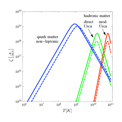
Figure 3: Bulk viscosity of unpaired nuclear matter from Urca processes with angular frequency $\omega=8.4\,{\rm kHz}$ and baryon density $n=2n_{0}$, taken from Ref. Alford et al. (2010a). If the direct Urca process is allowed, the reaction rate is faster and the maximum of the bulk viscosity is at a lower temperature. The dashed lines are obtained by using non-interacting matter for the susceptibilities, while the solid curves use the equation of state of Akmal et al. (1998). The plot also shows the result for unpaired, strange quark matter from the non-leptonic process $u+d\leftrightarrow u+s$, to be discussed in Sec. V.4.1, see also Fig. 5. Again, the dashed curve represents non-interacting quark matter, while the solid curve includes effects of the interaction on the thermodynamics.

We show the bulk viscosity of hadronic matter in Fig. 3. If the direct Urca process is allowed, the conversion of neutrons into protons and vice versa is faster and thus the maximum of the bulk viscosity occurs at a smaller temperature compared to the case where only the modified Urca process is at work. Since the strong interaction is needed for the modified Urca process, the corresponding rates are prone to large uncertainties, as discussed in the previous section. The bulk viscosity due to the modified Urca process used by Alford et al. (2010a), from which Fig. 3 is taken, is based on free one-pion exchange interaction Friman and Maxwell (1979); Haensel (1992); Reisenegger (1995). Kolomeitsev and Voskresensky (2015) showed that medium modifications in the MOPE model can enhance the rate of the modified Urca process and thus may shift the maximum of the bulk viscosity to lower temperatures. Fig. 3 also includes a comparison with quark matter, whose bulk viscosity we discuss in Sec. V.4. We see that the bulk viscosity peaks at even lower temperatures than that of hadronic matter with the direct Urca process. The reason is that in (unpaired) quark matter the more efficient non-leptonic, strangeness-changing, process $u+d\leftrightarrow u+s$ is the dominant chemical re-equilibration process. The figure also shows that the equation of state, through the susceptibilities $B$ and $C$, has a sizable effect on the bulk viscosity. This effect has also been studied by Vidaña (2012), with an emphasis on the role of the symmetry energy for the bulk viscosity.

The bulk viscosity also receives contribution from muons. Muons appear in the direct (or modified) Urca processes (124) with electron and electron neutrino replaced by muon and muon neutrino Haensel et al. (2000, 2001). One can also consider the purely leptonic processes that convert an electron into a muon and vice versa,

$$e+e\leftrightarrow\mu+e+\nu+\bar{\nu}\,,\qquad e+\mu\leftrightarrow\mu+\mu+\nu+\bar{\nu}\,.$$ (130)

These processes are the dominant contribution to the bulk viscosity for temperatures well below the critical temperature for hadronic superfluidity Alford and Good (2010).

As the result for quark matter in Fig. 3 suggests, the presence of strangeness has a significant effect on the bulk viscosity. The reason is that the phase space for a non-leptonic (strangeness-changing) process is typically much larger than that for a semi-leptonic process because the leptons have a negligibly small Fermi momentum. In hadronic matter, the presence of hyperons thus leads to a very different result for the bulk viscosity, with a maximum typically at smaller temperatures that for ordinary nuclear matter. The bulk viscosity based on the strangeness-changing processes

$$n+n \leftrightarrow p+\Sigma^{-}\,,$$ (131a)

$$n+p \leftrightarrow p+\Lambda\,,$$ (131b)

$$n+n \leftrightarrow n+\Lambda\,,$$ (131c)

has been computed by Jones (2001); Haensel et al. (2002); Lindblom and Owen (2002); van Dalen and Dieperink (2004); Chatterjee and Bandyopadhyay (2006). Effects of a large magnetic field were taken into account by Sinha and Bandyopadhyay (2009), and the bulk viscosity in quark/hadron mixed phases was computed by Drago et al. (2005).

The curves in Fig. 3 show the result for unpaired matter. Cooper pairing of nucleons and/or hyperons change the underlying reaction rates dramatically and (to a much smaller extent) the susceptibilities that enter the bulk viscosity. Therefore, the energy gap in the nucleon dispersions has to be taken into account, leading to a suppression of the reaction rates. This suppression is exponential for temperatures much smaller than the critical temperature if at least one of the participating particles [say the neutron or the proton for the direct Urca process (124)] is gapped with an isotropic gap. A power law suppression occurs if the pairing leaves a node at the Fermi sphere where excitations with infinitesimally small energy are possible. This is conceivable for certain phases of ${}^{3}P_{2}$ pairing of neutrons (the milder suppression is of course only possible if at the same time there are unpaired protons). As a consequence of the suppression of the reaction rate, the bulk viscosity is suppressed for small temperatures $T\ll T_{c}$. The effect of pairing on the bulk viscosity of hadronic matter was calculated by Haensel et al. (2000, 2001, 2002). If neutrons form a superfluid, the corresponding Goldstone mode may contribute to the bulk viscosity and, depending on the equation of state, there may be a temperature regime where its contribution is dominant Manuel et al. (2013). Superfluidity also has an effect on the hydrodynamics of the system. Since a superfluid at finite temperature is effectively a two-fluid system, there is more than a single bulk viscosity coefficient. The additional coefficients have been computed for superfluid nuclear matter from Urca processes by Gusakov (2007), from phonons by Manuel et al. (2013), and for superfluid nucleon-hyperon matter by Gusakov and Kantor (2008). The effect of these additional coefficients on the instability window for $r$-mode oscillations appears to be small Haskell and Andersson (2010).

V Transport in the core: quark matter

V.1 General remarks

Matter at sufficiently large baryon density is deconfined and quarks and gluons rather than baryons and mesons become the relevant degrees of freedom. This phase of matter is called quark matter or, especially at large temperatures where the gluons contribute to the thermodynamics, quark-gluon plasma. In the context of neutron stars, by quark matter we always mean three-flavor quark matter (or ‘strange quark matter’) made of up, down, and strange quarks. The reason is that the charm, bottom, and top quarks are too heavy to exist at the densities and temperatures typical for a neutron star. Therefore, even when we use perturbative methods which can only be trusted at extremely large densities, we ignore the heavy flavors because eventually we are interested in extrapolating our results down to neutron star densities. It is uncertain whether quark matter exists in the interior of neutron stars because we do not precisely know the central density of the star and, more importantly, we do not know the critical density at which nuclear matter turns into quark matter. It is conceivable that this transition is a crossover Schäfer and Wilczek (1999); Alford et al. (1999a); Hatsuda et al. (2006); Schmitt et al. (2011), such that there is no well-defined transition density, just like the transition from the hadronic phase to the quark-gluon plasma at large temperatures and small baryon densities Aoki et al. (2006). Astrophysical data may provide important clues for the question of the location and nature of the deconfinement transition at large densities. Connecting observations from neutron stars to properties of ultra-dense matter is an intriguing example of probing our understanding of fundamental theories such as QCD with the help of astrophysics. In the case of quark matter (and also ultra-dense nuclear matter), the interplay between astrophysics and theory is particularly important because currently there is no rigorous first-principle calculation of dense QCD, unless we go to even larger densities where perturbative methods become reliable Kurkela et al. (2010a, b); Kurkela et al. (2014). The reason is that even brute force methods on the lattice fail due to the so-called sign problem, although there has been recent progress towards evading and/or mitigating the sign problem Aarts (2016); Glesaaen et al. (2016); Gattringer and Langfeld (2016). Ideally, we would like a given phase of dense matter to be identifiable in an unambiguous way from a set of astrophysical observations. Of course, in reality, several distinct phases may show very similar behavior with respect to the observables that are accessible to us. For instance, many of the quark matter phases that we discuss in the following are basically indistinguishable from each other through bulk properties such as the equation of state and thus mass and radius of the star. But they do differ from each other in their low-energy properties, for instance because of different Cooper pairing patterns. Therefore, it is mostly the transport, less the thermodynamics, that differs from phase to phase.

When we compute transport properties of quark matter, many aspects are similar to what we have discussed for hadronic matter in the previous sections: we are obviously interested in the same quantities, i.e., neutrino emissivity, viscosity coefficients, etc., and the methods we use are often the same, even though the formulations in the literature may sometimes look different. Nevertheless, there are some general differences which are useful to keep in mind before we go into more details. Firstly, quark matter is relativistic because the quark masses are small compared to the quark chemical potential and thus compared to the Fermi momentum. (For the up and down quarks, the Fermi velocity $v_{F}$ introduced in Eq. (36) is very close to the speed of light, while the strange quark is heavy enough to induce sizable corrections to this ultra-relativistic limit.) Therefore, all microscopic calculations are performed in a relativistic framework, which for nuclear matter is only necessary at very large densities where the nucleon rest mass becomes comparable to the Fermi energy. Secondly, when we want to treat quark matter rigorously with currently available methods, we need to approach neutron star densities ‘from above’, i.e., we often assume quarks to be weakly interacting to be able to apply perturbation theory and then extrapolate the results down in density. This becomes relevant for some of the results discussed here, but not for all since, as we know from the previous section, not all transport properties rely on a precise knowledge of the strong interaction and are rather dominated by the electroweak interaction. Thirdly, quark matter has a larger variety of candidate phases for neutron star cores than nuclear matter because there are 9 fermion species in three-flavor, three-color quark matter. As a result, there is a multitude of different possible patterns of Cooper pairing Alford et al. (2008a), which is particularly interesting with regard to transport properties.

We will summarize the current state of the art of reaction rates and transport properties in quark matter that are relevant for neutron stars. We attempt to give a comprehensive account of the current knowledge, which is possible because there are considerably fewer studies about quark matter transport than about nuclear matter transport. The results about quark matter we present here were obtained starting from a few works in the early eighties through a peak period around 2005 – 2008 and including very recent progress that is still ongoing, with interesting ideas and prospectives for future work.

V.2 Phases of quark matter: overview

As a preparation, especially for readers unfamiliar with dense QCD, it is useful to start with a brief overview about the relevant quark matter phases and their basic properties. In many cases, these basic properties already give us a rough idea about the behavior of the transport properties which we shall then discuss in more detail.

Just as we know the properties of low-density ‘ordinary’ nuclear matter, we have solid, albeit only theoretical, knowledge about quark matter at extremely high densities. If the density is sufficiently large to apply weak-coupling methods and to neglect all three quark masses compared to the quark chemical potential, the ground state is the color-flavor locked (CFL) phase Alford et al. (1998, 1999b). While in nuclear matter more complicated phases including meson condensates and hyperons may occur as we move away from ordinary nuclear matter to larger densities (towards the center of the neutron star), more complicated phases of quark matter occur as we move towards lower densities (starting from the asymptotically dense regime, which is beyond neutron star densities).

In the CFL phase, all quarks participate in Cooper pairing, and as a consequence the dispersions of all fermionic quasiparticles are gapped. At zero temperature, the number densities of all quark species are identical, and therefore the CFL phase is ‘automatically’ neutral, without any electrons or muons (recall that the electric charges of up, down and strange quarks happen to add up to zero). This makes CFL very special with respect to transport because at low energies all fermionic degrees of freedom are suppressed and can be neglected. The CFL phase breaks chiral symmetry spontaneously, and thus there is a set of (pseudo-)Goldstone modes, very similar to the mesons that arise from ‘usual’ chiral symmetry breaking through a chiral condensate. At low temperatures, these light bosons dominate (some of) the transport properties of the CFL phase. The CFL mesons appear with the same quantum numbers as the mesons from quark-antiquark condensation, which is a consequence of the identical symmetry breaking pattern. However, their masses are different: in CFL, the kaons, not the pions, are the lightest mesons.

The CFL phase is a superfluid because it spontaneously breaks the $U(1)$ symmetry associated with baryon number conservation, and thus, as discussed in Sec. II.3.4, the usual complications of superfluid transport arise, such as the two-fluid picture at nonzero temperature, or the existence of quantized vortices in rotating CFL. Moreover, superfluidity implies the existence of an exactly massless Goldstone mode, which yields the dominant contribution for instance to the shear viscosity of CFL. The transport properties of CFL are determined by an effective theory for the pseudo-Goldstone modes and the superfluid mode. The form of this effective theory, in turn, is entirely given by the symmetry breaking pattern of CFL, just like usual chiral perturbation theory. Therefore, if CFL persists down to neutron star densities, we have a very solid knowledge of the low-energy physics of quark matter, although the numerical coefficients of the effective theory can only be determined reliably at weak coupling and become uncertain as we move towards lower densities.

The opposite of CFL, in a way, is unpaired quark matter, where none of the quark species forms Cooper pairs. Unpaired quark matter probably exists only at high temperatures $T\gtrsim 10\,{\rm MeV}$, because at lower temperatures Cooper pairing in some form seems unavoidable Alford et al. (2008a). Nevertheless, unpaired quark matter is an important concept and its transport properties, even at low temperature, are relevant. The reason is that almost all quark matter phases except for CFL have some unpaired quarks or quarks with a very small pairing gap, which dominate transport. Thus, up to numerical prefactors, the result for unpaired quark matter is a good approximation for these phases in many instances. The calculation of transport properties for unpaired quark matter is, in a sense, more difficult than for CFL because we need to know the interaction via gluons in a strongly coupled regime (unless the transport property of interest is dominated by the electroweak interactions). Therefore, shear viscosity, electrical and thermal conductivities of unpaired quark matter are typically based on perturbative calculations, assuming the strong coupling constant $\alpha_{s}$ to be small.

Between the two extreme cases of CFL (present at asymptotically large densities and sufficiently small temperatures) and completely unpaired quark matter (strictly speaking only present at temperatures higher than in a neutron star but important conceptually), there are many possible quark matter phases where quarks ‘partially’ pair. These phases are likely to be relevant for neutron stars and thus their transport properties have been studied extensively. ‘Partial’ pairing means that certain quark colors or flavors remain unpaired and/or that Cooper pairing does not occur in all directions in momentum space and even may vary spatially. Such phases necessarily appear at moderate densities because going down in density means a decrease in quark chemical potential and an increase in the strange quark mass, somewhere between the current mass of about $100\,{\rm MeV}$ and the vacuum constituent mass of about $500\,{\rm MeV}$. As a consequence, the strange quark mass cannot be neglected at densities in the cores of neutron stars, and the particularly symmetric situation at asymptotically large densities is disrupted. Why does the less symmetric situation of different quark masses eventually lead to a breakdown of CFL? The reason is that the gain in free energy from Cooper pairing is maximized if the two participating fermion species have the same Fermi surface and pairing occurs over the entire surface in momentum space. If the fermions that ‘want’ to pair have different Fermi surfaces, an energy cost is involved in Cooper pairing, and this cost may be too large to create a paired state. Different masses, together with the conditions of beta-equilibrium and charge neutrality, provide such a difference in Fermi surfaces because, at least for the most favorable spin-0 channel, pairing takes place between quarks of different color and flavor. Therefore, CFL is under stress if we move away from asymptotically large densities. The system is expected to react in a series of phase transitions, producing more complicated quark matter phases. The exact sequence of these phases can be determined in a controlled way at very large densities and weak coupling, but as we move to lower densities, we have less rigorous knowledge of the phase structure and rely mostly on model calculations or bold extrapolations from ultra-high densities. In particular, it is not known where in this sequence of phases nuclear matter takes over. It is conceivable that CFL persists down to densities where the transition to hadronic matter occurs, possibly leading to a nuclear/CFL interface inside a neutron star. It is also possible that other color-superconducting phases exist in the core of neutron stars, possibly breaking rotational and/or translational invariance. Also, since the QCD coupling increases with lower energies, $\alpha_{s}\gtrsim 1$ at densities relevant for astrophysics, the color-superconducting phases may be replaced by something qualitatively different, possibly involving elements from the Bardeen-Cooper-Schrieffer–Bose-Einstein-condensation (BCS-BEC) crossover Deng et al. (2007) seen in atomic gases or possibly showing features of the quarkyonic phase that is predicted in QCD in the limit of infinite number of colors $N_{c}$ McLerran and Pisarski (2007).

V.3 Neutrino emissivity

As for hadronic matter, neutrino emissivity is interesting in itself because it is the main cooling mechanism of the star, and the rates for the neutrino processes can be relevant for the bulk viscosity of quark matter inside a neutron star. We consider the processes

$$d\to u+e+\bar{\nu}_{e}\,,\qquad u+e\to d+\nu_{e}\,.$$ (132)

These are the analogues of the direct Urca processes in nuclear matter (95). In quark matter, the triangle inequality from momentum conservation does not pose a severe constraint on this process because the Fermi surfaces between up and down quark are not as different as the ones for neutrons and protons in nuclear matter. Therefore, second-order neutrino processes such as bremsstrahlung are usually negligible in quark matter. We first discuss the processes (132) and later summarize the results that involve strangeness. Generalizing the definition (99), where Fermi’s Golden Rule was applied directly, the neutrino emissivity is

$$\epsilon_{\nu}\equiv 2\frac{\partial}{\partial t}\int\frac{d^{3}{\bm{p}}_{\nu}}{(2\pi)^{3}}\,p_{\nu}\,f_{\nu}(t,{\bm{p}}_{\nu})\,,$$ (133)

where ${\bm{p}}_{\nu}$ is the neutrino momentum, and the factor 2 accounts for neutrinos and anti-neutrinos. The change of the neutrino distribution function $f_{\nu}$ is computed from the gain term in the neutrino transport equation, which takes the form

$$\frac{\partial}{\partial t}f_{\nu}(t,{\bm{p}}_{\nu}) = -\frac{\cos^{2}\theta_{C}G_{F}^{2}}{8}\int\frac{d^{3}{\bm{p}}_{e}}{(2\pi)^{3}p_{\nu}p_{e}}L_{\lambda\sigma}f_{F}(p_{e}-\mu_{e})f_{B}(p_{\nu}+\mu_{e}-p_{e}){\rm Im}\,\Pi_{R}^{\lambda\sigma}(Q)\,,$$ (134)

with the Fermi and Bose distribution functions $f_{F,B}(x)=(e^{x/T}\pm 1)^{-1}$ for the electron with energy $p_{e}$ and chemical potential $\mu_{e}$ and the $W$-boson with four-momentum $Q=(q_{0},{\bm{q}})=(p_{e}-p_{\nu}-\mu_{e},{\bm{p}}_{e}-{\bm{p}}_{\nu})$. We have abbreviated $L^{\lambda\sigma}\equiv\mbox{Tr}\left[(\gamma_{0}p_{e}-\bm{\gamma}\cdot{\bm{p}}_{e})\,\gamma^{\sigma}(1-\gamma^{5})(\gamma_{0}p_{\nu}-\bm{\gamma}\cdot{\bm{p}}_{\nu})\,\gamma^{\lambda}(1-\gamma^{5})\right]$, with the Dirac matrices $\gamma^{\sigma}$ ($\sigma=0,1,2,3$) and $\gamma^{5}=i\gamma^{0}\gamma^{1}\gamma^{2}\gamma^{3}$. (Note that the subscript $\nu$ stands for neutrino and is thus not used as a Lorentz index.) Finally, ${\rm Im}\,\Pi_{R}^{\lambda\sigma}$ is the imaginary part of the retarded $W$-boson self-energy

$$\Pi^{\lambda\sigma}(Q)=\frac{T}{V}\sum_{K}\mbox{Tr}[\Gamma_{-}^{\lambda}S(K)\Gamma_{+}^{\sigma}S(P)]\,,$$ (135)

with the quark propagator $S$, which is a matrix in color, flavor, and Dirac space and – in the case of Cooper pairing – in Nambu-Gorkov space. The electroweak vertices are diagonal in Nambu-Gorkov space, $\Gamma_{\pm}^{\lambda}={\rm diag}[\gamma^{\lambda}(1-\gamma^{5})\tau_{\pm},-\gamma^{\lambda}(1+\gamma^{5})\tau_{\mp}]$, where $\tau_{\pm}=(\tau_{1}\pm i\tau_{2})/2$ with the Pauli matrices $\tau_{1}$, $\tau_{2}$ are matrices in flavor space which ensure that an up and a down quark interact at the vertex, i.e., $K$ and $P$ correspond to the up and down quark four-momenta, respectively.

As an instructive example for the neutrino emissivity in quark matter due to the Urca processes, let us discuss the 2SC phase Bailin and Love (1984). In the 2SC phase all strange quarks and all quarks of one color, say blue, are ungapped. This phase is an example for the less symmetrically paired phases mentioned above. The up and down quarks participating in the processes (132) can be either gapped or ungapped. Since the weak interaction does not change the color of the quarks, they are either both gapped (when they are red or green) or both ungapped (when they are blue). The contribution of the gapped sector, here shown for a single color, is Schmitt (2010)

$$\frac{\partial}{\partial t}f_{\nu}(t,{\bm{p}}_{\nu}) = \frac{\pi\cos^{2}\theta_{C}G_{F}^{2}}{4}\sum_{e_{1},e_{2}=\pm}\int\frac{d^{3}{\bm{p}}_{e}d^{3}{\bm{k}}}{(2\pi)^{3}(2\pi)^{3}p_{\nu}p_{e}}L_{\lambda\sigma}\left({\cal T}^{\lambda\sigma}B_{k}^{e_{1}}B_{p}^{e_{2}}+{\cal U}^{\lambda\sigma}\frac{\Delta^{2}}{4\varepsilon_{k}\varepsilon_{p}}\right)$$ (136)

$$\times f_{F}(p_{e}-\mu_{e})f_{F}(-e_{1}\varepsilon_{k})f_{F}(e_{2}\varepsilon_{p})\delta(q_{0}-e_{1}\varepsilon_{k}+e_{2}\varepsilon_{p})\,,$$

where ${\bm{k}}$ and ${\bm{p}}$ are the up and down quark three-momenta, respectively. We have denoted the Bogoliubov coefficients by $B_{k}^{e}=(1-e\xi_{k}/\varepsilon_{k})/2$ with $\xi_{k}=k-\mu_{u}$ and the quasiparticle dispersion $\varepsilon_{k}^{2}=\xi^{2}_{k}+\Delta^{2}$, where $\mu_{u}$ is the up quark chemical potential, and analogously for the down quark with chemical potential $\mu_{d}$. Moreover, we have abbreviated ${\cal T}^{\lambda\sigma}\equiv{\rm Tr}\left[\gamma^{\lambda}(1-\gamma^{5})\gamma^{0}\Lambda_{k}^{-}\gamma^{\sigma}(1-\gamma^{5})\gamma^{0}\Lambda_{p}^{-}\right]$, and ${\cal U}^{\lambda\sigma}\equiv{\rm Tr}\left[\gamma^{\lambda}(1-\gamma^{5})\gamma^{5}\Lambda_{k}^{+}\gamma^{\sigma}(1+\gamma^{5})\gamma^{5}\Lambda_{p}^{-}\right]$, with the energy projectors $\Lambda_{k}^{\pm}=(1\pm\gamma^{0}\bm{\gamma}\cdot\hat{\bm{k}})/2$. The contribution proportional to $\Delta^{2}$ comes from the so-called anomalous propagators, the off-diagonal components of the quark propagator $S(K)$ in Nambu-Gorkov space. Their effect was discussed in detail and evaluated numerically for the 2SC phase by Jaikumar et al. (2006), see Fig. 4 for a diagrammatic representation of normal and anomalous contributions to the $W$-boson self-energy.

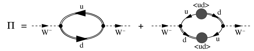
Figure 4: Normal and anomalous contributions to the $W$-boson self-energy needed to compute the neutrino emissivity in the presence of Cooper pairing, here shown for pairing between up and down quarks, for instance in the 2SC phase. The first diagram contains two ‘normal’ propagators (diagonal elements in Nambu-Gorkov space), the double line indicating that they include the effect of pairing through a modified dispersion relation. The second diagram contains two ‘anomalous’ propagators (off-diagonal elements in Nambu-Gorkov space), whose diagrammatic structure indicates that they describe a propagating fermion that is absorbed by the condensate $\langle ud\rangle$ and continues to propagate as a charge-conjugate fermion. The two contributions are obtained naturally in the Nambu-Gorkov formalism by performing the trace over Nambu-Gorkov space in Eq. (135).

The expression in Eq. (136) is instructive for the neutrino emissivity in the presence of Cooper pairing because it shows 4 potential subprocesses that arise from summing over $e_{1}$ and $e_{2}$. Naively, one would expect the distribution functions for the process $u+e\to d+\nu_{e}$ to appear in the form $f_{e}f_{u}(1-f_{d})$ (we have neglected $f_{\nu}$ since the neutrinos leave the star once they are created). We see that the combinations $f_{e}f_{u}f_{d}$, $f_{e}(1-f_{u})(1-f_{d})$, $f_{e}(1-f_{u})f_{d}$ appear as well [note that for the Fermi distribution $f(-x)=1-f(x)$]. The reason is that quasiparticles in the superconductor are mixtures of particles and holes (this momentum-dependent mixture is quantified by the Bogoliubov coefficients) and are thus allowed to appear on either side of the reaction. Since we have started from a general form of the reaction rate that is based on the full structure of the propagator, all four reactions are included automatically and we do not have to set up a separate calculation of these Cooper pair breaking and formation processes. This is analogous to nuclear matter with superfluid neutrons, see Sec. IV.2.3. In that case, since the direct Urca process is usually suppressed, the Cooper pair breaking and formation processes are discussed for the neutral current process $n+n\to n+n+\nu+\bar{\nu}$, which, in the presence of Cooper pairing, allows for the processes $\{nn\}\to n+n+\nu+\bar{\nu}$ and $n+n\to\{nn\}+\nu+\bar{\nu}$, where $\{...\}$ denotes the Cooper pair condensate. The quark version of these processes is $\{uu\}\to u+u+\nu+\bar{\nu}$ and $u+u\to\{uu\}+\nu+\bar{\nu}$ (assuming single-flavor quark Cooper pairing), which yields a neutrino emissivity $\epsilon_{\nu}\propto T^{7}$ Jaikumar and Prakash (2001), just like in nuclear matter.

If we are only interested in small temperatures compared to the energy gap $\Delta$, the Cooper pair breaking and formation processes are irrelevant, and the contribution from the gapped quarks is exponentially suppressed, $\epsilon_{\nu}\propto e^{-\Delta/T}$. As a consequence, the neutrino emissivity of the 2SC phase is, at small temperatures, utterly dominated by the unpaired blue quarks. At higher temperatures, as we approach the critical temperature $T_{c}$ (for the 2SC phase, $T_{c}\sim 10\,{\rm MeV}$), Eq. (136) has to be evaluated numerically.

To compute the neutrino emissivity for unpaired quarks, we may set $\Delta=0$ in Eq. (136). As a result, the dispersions $\varepsilon_{k}$ of the quarks (assumed to be massless) become dispersions of free fermions. However, it is crucial to include the effect of the strong interaction, i.e., to treat the system as a Fermi liquid rather than a non-interacting system of quarks. Otherwise, the phase space for the Urca process is zero and the neutrino emissivity vanishes. Fermi liquid corrections are included by writing the Fermi momenta of up and down quarks as $\mu_{u}[1-{\cal O}(\alpha_{s})]$ and $\mu_{d}[1-{\cal O}(\alpha_{s})]$. The result for 2-flavor unpaired quark matter is (reinstating all color degrees of freedom, $N_{c}=3$)

$$\epsilon_{\nu}^{\rm unp.}\approx\frac{457}{630}\cos^{2}\theta_{C}G_{F}^{2}\alpha_{s}\mu_{e}\mu_{u}\mu_{d}T^{6}\left(1+\frac{4\alpha_{s}}{9\pi}\ln\frac{\Lambda}{T}\right)^{2}\,,$$ (137)

where the electron chemical potential is related to the quark chemical potentials via $\mu_{u}+\mu_{e}=\mu_{d}$ in $\beta$-equilibrium. The logarithmic correction of Schäfer and Schwenzer (2004) to the standard result by Iwamoto (1980, 1982) arises if non-Fermi liquid effects are included for the quarks, and can lead to an enhancement of the neutrino emissivity at low temperatures Schäfer and Schwenzer (2004). The energy scale that appears in the logarithm is of the order of the screening scale, $\Lambda\propto g\mu$, where $g$ is the strong coupling constant related to $\alpha_{s}$ by $\alpha_{s}=g^{2}/(4\pi)$, see Ref. Gerhold and Rebhan (2005) for a calculation of $\Lambda$. Higher order corrections to this result have been computed by Adhya et al. (2012). The strange quark mass has to be included if the result is generalized to strange quark matter. A mass term can easily be added in the quark dispersion, but the result for the emissivity becomes more complicated and is best evaluated numerically. One effect of the mass is to open up the phase space such that the emissivity would be nonzero even if the Fermi liquid corrections were neglected, as discussed by Iwamoto (1980); Wang et al. (2006). A dynamical quark mass from a chiral density wave has a similar effect. The chiral density wave is an anisotropic phase in which the chiral condensate oscillates between between scalar and pseudoscalar components, and the neutrino emissivity depends on the dynamical mass and the wave vector that determines this oscillation Tatsumi and Muto (2014). This phase, possibly in coexistence with quark Cooper pairing is a candidate phase in the vicinity of a potential first-order chiral phase transition between the hadronic matter and quark matter.

A similar calculation as outlined here for the unpaired and 2SC phases applies to the so-called Larkin-Ovchinnikov-Fulde-Ferrell (LOFF) phases and to color superconductors where Cooper pairs have total spin one. These two classes of phases are further important examples of the less symmetric phases that are expected to arise for a large mismatch in Fermi surfaces. An estimate of this mismatch, based on an expansion for small strange quark masses $m_{s}$, is given by comparing $m_{s}^{2}/\mu$ to the energy gap $\Delta$, where $\mu$ is the quark chemical potential (baryon chemical potential divided by $N_{c}=3$). In neutron stars, exotic phases like LOFF or spin-one pairing thus occur if the attractive interaction (for which $\Delta$ is a measure) is not strong enough to overcome the mismatch $m_{s}^{2}/\mu$ (which increases with decreasing density because $m_{s}$ increases and $\mu$ decreases). In the LOFF phase, the system reacts to the mismatch in Fermi surfaces by forming Cooper pairs only in certain directions in momentum space, resulting in Cooper pairs with nonzero momentum Alford et al. (2001); Anglani et al. (2014). In general, a finite number of different Cooper pair momenta will be realized in a given phase, resulting in counter-propagating currents and in a crystalline structure with periodically varying gap function. Since there are directions in momentum space where the quasiparticle dispersion is ungapped, the neutrino emissivity of the LOFF phase is qualitatively very similar to unpaired quark matter, as shown by Anglani et al. (2006). Spin-one color superconductors arise unavoidably in single-flavor Cooper pairing. This form of pairing is the only possible one if the mismatch in Fermi momenta of quarks of different flavor is sufficiently large to prevent any form of cross-flavor pairing. Spin-one color superconductors break rotational symmetry and typically exhibit ungapped directions in momentum space as well. Therefore, as for the LOFF phase, their neutrino emissivity has the same $T^{6}$ behavior as unpaired quark matter. A possible exception is the color-spin locked phase (CSL), where, in a certain variant, all quarks are gapped. However, weak coupling calculations suggest that another variant of CSL, where there are unpaired quasifermions, is energetically preferred Schmitt (2005) (although there are fewer paired quarks, the larger value of the gap function overcomes this lack of pairing). If we only consider the gapped branches, there are striking similarities of the neutrino emissivity in spin-one color superconductors, computed by Schmitt et al. (2006); Wang et al. (2006); Berdermann et al. (2016), to the neutrino emissivity of ${}^{3}P_{2}$ phases in nuclear matter Yakovlev et al. (2001), which we have briefly discussed in Sec. IV.2.3.

The neutrino emissivity of CFL is qualitatively different from the phases with ungapped fermions. In CFL, neutrino emissivity is dominated by the Goldstone modes, and the relevant processes are

$$\pi^{\pm},K^{\pm}\to e^{\pm}+\bar{\nu}_{e}\,,\qquad\pi^{0}\to\nu_{e}+\bar{\nu}_{e}\,,\qquad\phi+\phi\to\phi+\nu_{e}+\bar{\nu}_{e}\,.$$ (138)

Here, $\pi^{\pm}$ and $K^{\pm}$ are the CFL mesons mentioned above, which have the same quantum numbers as, but different masses than, their counterparts from usual chiral symmetry breaking. In particular, the kaons are the lightest mesons in CFL, with masses of a few MeV. Since these masses are larger than typical temperatures of neutron stars, the resulting neutrino emissivities are exponentially suppressed. The superfluid mode $\phi$ is massless and thus does not show this exponential suppression. However, the emissivity is proportional to a large power of $T$, which makes this result very small as well Jaikumar et al. (2002),

$$\epsilon_{\nu}^{\rm CFL}\sim\frac{G_{F}^{2}T^{15}}{f_{\phi}\mu^{4}}\,,$$ (139)

where $f_{\phi}$ is the analogue of the pion decay constant for the spontaneous breaking of baryon number. We conclude that the CFL phase basically does not contribute to the neutrino emissivity.

Neutrino emissivities of quark matter have been included in cooling calculations for hybrid stars Grigorian et al. (2005); Popov et al. (2006); Hess and Sedrakian (2011); Noda et al. (2013), and quark matter may provide an explanation for the rapid cooling of the neutron star in Cassiopeia A Sedrakian (2013, 2016a). In this scenario, the star cools through a transition from the 2SC phase with very inefficient cooling to a crystalline color superconductor, where there are unpaired fermions. This explanation assumes that there is no contribution of the strange quarks and – on purely phenomenological grounds – that there is some residual pairing mechanism for the blue quarks in 2SC. While the explanation of the rapid cooling in nuclear matter is based on the transition from an unpaired phase to the superfluid phase, quark matter may thus potentially show a similar behavior via a transition from one paired phase to another.

V.4 Bulk viscosity

V.4.1 Unpaired quark matter

We have already discussed the definition and physical meaning of the bulk viscosity $\zeta$ in Sec. IV.3 and can immediately start from the expression

$$\zeta=-\frac{2}{\omega^{2}\delta v_{0}^{2}}\frac{1}{\tau}\int_{0}^{\tau}dt\,P(t)\frac{d\delta v}{dt}\,,$$ (140)

which follows from Eqs. (121) and (122). The pressure $P(t)$ is given by Eq. (123), where now, for unpaired quark matter, the oscillations in density occur for the three quark flavors and the electron, $\delta n_{u}$, $\delta n_{d}$, $\delta n_{s}$, $\delta n_{e}$. We consider the processes

$$u+d \leftrightarrow u+s\,,$$ (141a)

$$u+e \to d+\nu_{e}\,,\qquad d\to u+e+\bar{\nu}_{e}$$ (141b)

$$u+e \to s+\nu_{e}\,,\qquad s\to u+e+\bar{\nu}_{e}\,.$$ (141c)

The non-leptonic process $u+d\leftrightarrow u+s$ will turn out to be the dominant one, but it is instructive to keep the leptonic processes. This allows us to sketch the calculation of the bulk viscosity for a more complicated scenario as outlined at the beginning of Sec. IV.3. Namely, we now have two out-of-equilibrium chemical potentials $\delta\mu_{1}\equiv\mu_{s}-\mu_{d}$ and $\delta\mu_{2}\equiv\mu_{d}-\mu_{u}-\mu_{e}$, relevant for the reactions (141a) and (141b). The relevant difference in chemical potentials for the reaction (141c) is then $\delta\mu_{1}+\delta\mu_{2}$, and thus not an independent quantity. As independent changes in densities we keep $\delta n_{d}$, $\delta n_{e}$. The changes in up and strange quark densities then are $\delta n_{u}=\delta n_{d}-\delta n_{e}$ and $\delta n_{s}=-\delta n_{d}-\delta n_{e}$. The change in the electron density comes from the processes (141b) and (141c), and the change in the down quark number density comes from the processes (141a) and (141b), and in analogy to Eq. (125) we write in the linear approximation

$$\frac{dn_{e}}{dt}\approx(\lambda_{2}+\lambda_{3})\delta\mu_{2}(t)+\lambda_{3}\delta\mu_{1}(t)\,,\qquad\frac{dn_{d}}{dt}\approx\lambda_{1}\delta\mu_{1}(t)-\lambda_{2}\delta\mu_{2}(t)\,,$$ (142)

where $\lambda_{1}$, $\lambda_{2}$, $\lambda_{3}$ have to be computed from the microscopic processes. The result for the non-leptonic process (141a) is Wang and Lu (1984); Sawyer (1989b); Madsen (1993)

$$\lambda_{1}\approx\frac{64\sin^{2}\theta_{C}\cos^{2}\theta_{C}G_{F}^{2}}{5\pi^{3}}\mu_{d}^{5}T^{2}\,,$$ (143)

while the leptonic processes (141b) and (141c) yield Iwamoto (1980, 1982)

$$\lambda_{2} \approx \frac{17\cos^{2}\theta_{C}G_{F}^{2}}{15\pi^{2}}\alpha_{s}\mu_{u}\mu_{d}\mu_{e}T^{4}\,,$$ (144a)

$$\lambda_{3} \approx \frac{17\sin^{2}\theta_{C}G_{F}^{2}}{40\pi^{2}}\mu_{s}m_{s}^{2}T^{4}\,,$$ (144b)

where $\lambda_{2}$ is obtained from the same calculation that leads to the neutrino emissivity (137), and the leptonic process including the strange quark is computed to lowest order in the strange quark mass $m_{s}$. Generalizing Eq. (126), we have two differential equations for $\delta\mu_{1}$ and $\delta\mu_{2}$,

$$\frac{d\delta\mu_{i}}{dt} = \frac{\partial\delta\mu_{i}}{\partial V}V_{0}\frac{d\delta v}{dt}+\sum_{x=u,d,s,e}\frac{\partial\delta\mu_{i}}{\partial n_{x}}\frac{dn_{x}}{dt}$$ (145)

$$= -B_{i}\frac{d\delta v}{dt}-\alpha_{i}\delta\mu_{1}(t)-\beta_{i}\delta\mu_{2}(t)\,,\qquad i=1,2\,,$$

where $B_{i}$ are combinations of thermodynamic functions in equilibrium, and $\alpha_{i}$, $\beta_{i}$ contain thermodynamic functions and the reaction rates $\lambda_{1}$, $\lambda_{2}$, $\lambda_{3}$. As in Sec. IV.3, we use the ansatz $\delta\mu_{i}(t)={\rm Re}(\delta\mu_{i0}e^{i\omega t})$ with complex amplitudes $\delta\mu_{i0}$, such that (145) can be solved for real and imaginary parts of $\delta\mu_{10}$ and $\delta\mu_{20}$. The bulk viscosity (140) then becomes

$$\zeta=\frac{a_{1}{\rm Re}(\delta\mu_{10})+a_{2}{\rm Re}(\delta\mu_{20})}{\omega^{2}\delta v_{0}}\,,$$ (146)

where $a_{1}$ and $a_{2}$ are combinations of $B_{1}$, $B_{2}$, $\lambda_{1}$, $\lambda_{2}$, $\lambda_{3}$. Computing ${\rm Re}(\delta\mu_{10})$ and ${\rm Re}(\delta\mu_{10})$ from Eq. (145) yields the final expression in terms of thermodynamic functions in equilibrium, the reaction rates, and the externally given frequency $\omega$. This result is very lengthy and entangles all reaction rates in a complicated way with the thermodynamic functions Alford and Schmitt (2007); Sa’d et al. (2007a).

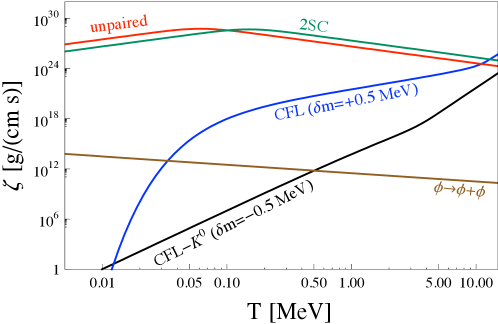
Figure 5: Bulk viscosity for unpaired quark matter, the 2SC phase, and the CFL phase. For the CFL phase, the result is shown from the process that only involves the superfluid mode $\phi$ and from processes that involve kaons and the superfluid mode, for thermal kaons $\delta m=m_{K^{0}}-\mu_{K^{0}}>0$ and condensed kaons $\delta m<0$. The parameters chosen here are the quark chemical potential $\mu=400\,{\rm MeV}$, the frequency $\omega/(2\pi)=1\,{\rm ms}^{-1}$, and the kaon mass $m_{K^{0}}=10\,{\rm MeV}$. The figure is reproduced with modifications from Ref. Alford et al. (2008b).

For a qualitative discussion we introduce the inverse time scales $\gamma_{\rm nl}=\lambda_{1}/\mu_{s}^{2}$ for the non-leptonic process (141a) and $\gamma_{\rm l}=\lambda_{2}/\mu_{s}^{2}\approx\lambda_{3}/\mu_{s}^{2}$ for the leptonic processes (141b) and (141c) and assume $\gamma_{\rm nl}\gg\gamma_{\rm l}$. Then, with some simple estimates of the thermodynamic functions, and ignoring numerical prefactors, we find Alford and Schmitt (2007)

$$\zeta\propto\gamma_{\rm nl}\frac{\gamma_{\rm nl}\gamma_{\rm l}+\omega^{2}}{\gamma_{\rm nl}^{2}\gamma_{\rm l}^{2}+\gamma_{\rm nl}^{2}\omega^{2}+\omega^{4}}\,.$$ (147)

From this result, various limit cases can be derived, depending on whether the external frequency $\omega$ is of the order of the leptonic rate, the nonleptonic rate, in between these rates etc. The most relevant case turns out to be $\omega\approx\gamma_{\rm nl}\gg\gamma_{\rm l}$, in which the slower leptonic processes can be completely neglected. Reinstating the thermodynamic functions, we obtain Madsen (1992)

$$\zeta\approx\frac{\lambda_{1}B^{2}}{(\lambda_{1}C)^{2}+\omega^{2}}\,,$$ (148)

where

$$B\equiv n_{d}\frac{\partial\mu_{d}}{\partial n_{d}}-n_{s}\frac{\partial\mu_{s}}{\partial n_{s}}\,,\qquad C\equiv\frac{\partial\mu_{d}}{\partial n_{d}}+\frac{\partial\mu_{s}}{\partial n_{s}}\,.$$ (149)

We have recovered the result (129) derived in the context of nuclear matter for a single reaction rate. The result for unpaired quark matter as a function of temperature for a fixed frequency $\omega$ is plotted in Fig. 5.

The calculation of the bulk viscosity in unpaired quark matter outlined here has been improved and extended in the literature in several ways. Firstly, Cooper pairing needs to be taken into account, and we shall discuss the results for various phases in the following subsection (Fig. 5 collects most of these results). Secondly, the supra-thermal regime, where the amplitude of the oscillations in chemical potential become large compared to the temperature, has been studied by Alford et al. (2010a), who have generalized earlier numerical results for strange quark matter by Madsen (1992). Shovkovy and Wang (2011) studied this regime together with the interplay of leptonic and non-leptonic processes. The bulk viscosity in the presence of large amplitudes is important if the time evolution and in particular the saturation of unstable $r$-modes is studied Alford et al. (2012). Thirdly, as for the neutrino emissivity, see Eq. (137), non-Fermi liquid effects can be included in the calculation of unpaired quark matter. Most importantly, they modify the result for the dominant non-leptonic process $u+d\leftrightarrow u+s$ Schwenzer (2012)

$$\lambda_{1}\approx\frac{64\sin^{2}\theta_{C}\cos^{2}\theta_{C}G_{F}^{2}}{5\pi^{3}}\mu_{d}^{5}T^{2}\left(1+\frac{4\alpha_{s}}{9\pi}\ln\frac{\Lambda}{T}\right)^{4}\,.$$ (150)

The correction factor has a higher power compared to the leptonic process that leads to the neutrino emissivity (137) because now 4, not 2 quarks participate in the process. If this result is extrapolated to realistic values of the strong coupling, $\alpha_{s}\sim 1$, the enhancement due to the long-range interactions is larger than for the emissivity. As a consequence, the maximum of the bulk viscosity – at a fixed frequency $\omega$ – is shifted to smaller temperatures. Alford and Schwenzer (2014) pointed out that this may have interesting consequences for the $r$-mode instability, see Fig. 6. We have to keep in mind, however, firstly, that completely unpaired quark matter is unlikely to exist in this (sufficiently cold) temperature regime because some form of Cooper pairing is expected to occur, and, secondly, that unpaired quark matter provides extremely efficient cooling due to the presence of direct Urca processes (137), which is difficult to reconcile with observations Chugunov et al. (2017). Finally, Huang et al. (2010) have computed the bulk viscosity for unpaired strange quark matter in the presence of a magnetic field, which induces an anisotropic bulk viscosity and, for very large fields, $B\gtrsim 10^{18}\,{\rm G}$, a hydrodynamical instability.

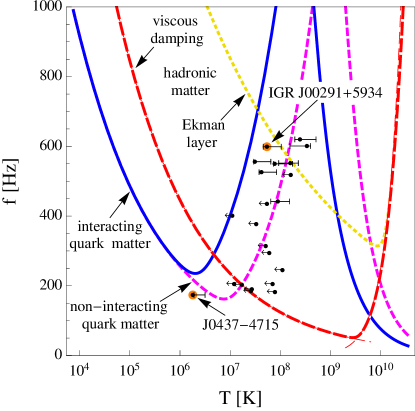
Figure 6: $R$-mode instability window, computed from bulk viscosity (high $T$) and shear viscosity (low $T$) in nuclear and quark matter, taken from Ref. Alford and Schwenzer (2014). Stars are unstable with respect to the emission of gravitational waves through the $r$-mode instability if they rotate with higher frequencies than given by the critical curves shown here. The observed pulsars shown as data points are in the stable region only for interacting quark matter with the non-Fermi-liquid corrections from Eq. (150). These corrections enhance the reaction rate for the conversion of down into strange quarks and thus shift the maximum of the bulk viscosity towards lower temperatures, leading to a shifted stability region compared to noninteracting quark matter. Hadronic matter is consistent with the data only by including additional processes such as dissipation from boundary layer rubbing at the crust of the star.

V.4.2 Color-superconducting quark matter

If Cooper pairing between the quarks is taken into account, the derivation outlined above is still valid, but the thermodynamic functions $B$ and $C$ in Eq. (148) become different, and of course the reaction rates (143) and (144) have to be recomputed. Let us first discuss the 2SC phase and its bulk viscosity from the process $u+d\leftrightarrow u+s$, which was computed by Alford and Schmitt (2007). Since the weak interaction does not change color, there are $N_{c}\times N_{c}=9$ subprocesses from the $N_{c}=3$ possible colors at each of the two electroweak vertices of the process $u+d\leftrightarrow u+s$. In the 2SC phase, only if the color at both vertices is blue, all participating quarks are ungapped. Therefore, at temperatures much smaller than the critical temperature $T_{c}$, where all processes with at least one gapped quark are exponentially suppressed, the reaction rate in the 2SC phase is 1/9 times the rate of unpaired quark matter. This does not necessarily mean that the bulk viscosity in the 2SC phase is smaller. It rather means that the maximum of the bulk viscosity, where the rate is in resonance with the frequency $\omega$, is assumed at a larger temperature (if the approximation $T\ll T_{c}$ is still valid at this temperature). The peak value of the bulk viscosity in the 2SC phase is different from the unpaired phase because the peak frequency is different and the thermodynamic functions $B$ and $C$ are different. It turns out, however, that for typical values of the strange quark mass and the superconducting gap, the peak values are very similar, as we can see in Fig. 5.

The bulk viscosity has also been computed in spin-one color superconductors, from the process $u+e\leftrightarrow d+\nu_{e}$ Sa’d et al. (2007b); Berdermann et al. (2016), which is the dominant one if strange quarks are ignored, and taking into account the non-leptonic process $u+d\leftrightarrow u+s$ Wang and Shovkovy (2010), whose reaction rate for four different spin-one color superconductors was computed by Wang et al. (2010). The conclusion is very similar as for the 2SC phase: since there are unpaired quarks in all possible spin-one phases (with the exception mentioned above in the context of neutrino emissivity), one can, for a rough estimate, neglect the contributions of the gapped branches, and the reaction rates become, up to a numerical prefactor, the same as for unpaired quark matter. The bulk viscosity thus behaves qualitatively similar to 2SC quark matter.

The CFL phase behaves differently because there are no ungapped quarks that can contribute to chemical re-equilibration processes, and the bulk viscosity is dominated from bosonic low-energy degrees of freedom, such as the kaon and the superfluid mode via the processes

$$K^{0} \leftrightarrow \phi+\phi\,,$$ (151a)

$$\phi \leftrightarrow \phi+\phi\,.$$ (151b)

The process involving the neutral kaon has been computed for thermal kaons by Alford et al. (2007). As mentioned above, the kaons are the lightest pseudo-Goldstone modes from chiral symmetry breaking in CFL. If the strange quark mass is taken into account, kaon condensation occurs on top of the Cooper pair condensation, giving rise to the so-called CFL-$K^{0}$ phase Bedaque and Schäfer (2002); Kaplan and Reddy (2002). This phase is the next phase down in density if we start from the CFL phase at asymptotically large densities and include the effects of the strange quark mass in a systematic way. It is therefore a very important phase and a viable candidate for the interior of neutron stars. The bulk viscosity of the CFL-$K^{0}$ phase is also dominated by the process (151a), where $K^{0}$ now denotes the Goldstone mode from kaon condensation Alford et al. (2008b); Schmitt (2008). This Goldstone mode would be exactly massless if strangeness was an exact symmetry. Taking into account the effect of the weak interactions, one finds a mass of about $50\,{\rm keV}$ for this mode Son (2001), smaller than the temperatures at which the bulk viscosity of the CFL-$K^{0}$ phase becomes sizable. Since all the above arguments about the bulk viscosity remain valid, the bulk viscosity of CFL also peaks at a certain temperature. In Fig. 5 we see that this maximum is reached only at temperatures larger than $10\,{\rm MeV}$. This is due to the less efficient reaction (151a) compared to contributions from quarks. Therefore, inside neutron stars, the CFL bulk viscosity, with or without kaon condensation, is very small compared to other quark matter phases. One might think that the potentially large result for the bulk viscosity at high temperatures is relevant for proto-neutron stars or neutron star mergers, where temperatures may well reach $10\,{\rm MeV}$ or more. However, we expect the critical temperatures for kaon condensation Alford et al. (2008c) and the critical temperature of CFL itself to be of the order of $10\,{\rm MeV}$, and thus the results beyond this temperature have to be taken with care.

At much lower temperatures, the process (151b), which only involves the exactly massless superfluid mode $\phi$, is expected to be dominant Manuel and Llanes-Estrada (2007). The result shown in Fig. 5 for this process should be taken seriously only for temperatures larger than about $50\,{\rm keV}$, because for smaller temperatures the mean free path is of the order of or larger than the size of the star, indicating that we are no longer in the hydrodynamic regime. Since the CFL phase is a superfluid, there is more than one bulk viscosity coefficient because a superfluid at nonzero temperature can be viewed as a two-fluid system, as mentioned in Sec. II.3.4. Let us denote the full relativistic stress-energy tensor of a superfluid by $T^{\mu\nu}_{\rm ideal}+T^{\mu\nu}_{\rm diss}$, as we did in Sec. II.3.3 for a normal fluid. Then, the dissipative terms in first-order hydrodynamics that are usually considered are

$$T^{\mu\nu}_{\rm diss} = \eta\Delta^{\mu\gamma}\Delta^{\nu\delta}\left(\partial_{\delta}v_{\gamma}+\partial_{\gamma}v_{\delta}-\frac{2}{3}g_{\gamma\delta}\partial\cdot v\right)+\Delta^{\mu\nu}\left[\zeta_{1}\partial_{\gamma}\left(\frac{n_{s}}{\sigma}w^{\gamma}\right)+\zeta_{2}\partial\cdot v\right]$$ (152)

$$+\kappa(\Delta^{\mu\gamma}v^{\nu}+\Delta^{\nu\gamma}v^{\mu})[\partial_{\gamma}T+T(v\cdot\partial)v_{\gamma}]\,.$$

We have denoted $\Delta^{\mu\nu}=g^{\mu\nu}-v^{\mu}v^{\nu}$ with the metric tensor $g^{\mu\nu}={\rm diag}(1,-1,-1,-1)$ and the four-velocity of the normal fluid $v^{\mu}$. Moreover, $n_{s}$ is the superfluid density, $w^{\mu}\equiv\partial^{\mu}\psi-\mu v^{\mu}$ with the chemical potential $\mu$ measured in the rest frame of the normal fluid and $\partial^{\mu}\psi/\sigma$ the four-velocity of the superfluid with the phase of the condensate $\psi$ and the chemical potential measured in the rest frame of the superfluid $\sigma=(\partial_{\mu}\psi\partial^{\mu}\psi)^{1/2}$. For a single fluid, $n_{s}=0$, Eq. (152) reduces to the normal-fluid expression (43b) with $\zeta=\zeta_{2}$. The Josephson equation, which relates the chemical potential $\mu$ to the phase of the condensate, is also modified by dissipative corrections,

$$v\cdot\partial\psi=\mu+\zeta_{3}\partial_{\mu}\left(\frac{n_{s}}{\sigma}w^{\mu}\right)+\zeta_{4}\partial\cdot v\,.$$ (153)

In general, there are even more possible dissipative terms and thus more coefficients in a two-fluid system Gusakov (2007), which are usually neglected. As mentioned in Sec. II.3.3, the form given here corresponds to the Eckart frame, where, in contrast to the Landau frame, there is no explicit dissipative correction to the conserved current. With $\zeta_{4}=\zeta_{1}$ due to the Onsager symmetry principle, there are three independent bulk viscosity coefficients $\zeta_{1}$, $\zeta_{2}$, $\zeta_{3}$ (which have different units), and $\zeta_{2}$ corresponds to $\zeta$ discussed above for a single fluid. The bulk viscosity coefficients have been estimated for the process (151b) in the zero-frequency limit by Mannarelli and Manuel (2010) with the result

$$\zeta_{1}\sim\frac{m_{s}^{2}}{T\mu}\,,\qquad\zeta_{2}\sim\frac{m_{s}^{4}}{T}\,,\qquad\zeta_{3}\sim\frac{1}{T\mu^{2}}\,,$$ (154)

and for the process (151a) by Bierkandt and Manuel (2011). The bulk viscosity coefficients of CFL have been applied to the damping of $r$-modes by Andersson et al. (2010), but, as argued above, the dissipative effects from bulk viscosity in CFL are very small. This is not changed by the additional bulk viscosity coefficients from superfluidity.

V.5 Shear viscosity, thermal and electrical conductivity

V.5.1 Unpaired quark matter

As we have already seen in Sec. IV, the physics behind shear viscosity of dense matter in neutron stars is different from the physics behind bulk viscosity. In the case of shear viscosity, it is thermal, not chemical, re-equilibration and thus for the baryonic and the quark contributions the strong, not the electroweak, interaction becomes relevant. (Recall, however, that even in the calculation of electroweak processes and chemical re-equilibration the strong interaction plays a role because the participating quarks interact strongly with each other.) Electrically neutral unpaired quark matter must contain electrons because the strange quark mass induces an imbalance between the number densities of up, down, and strange quarks, and electrons are needed to neutralize the system. We shall discuss the electron contribution in the context of the 2SC phase below, but first focus on the contribution from quarks alone. If we assume the QCD coupling to be weak, the quasiparticle picture is valid and we can use a kinetic approach to compute the quark-quark scattering rate from one-gluon exchange. This calculation proceeds along the same lines as outlined in Sec. IV.1. Here we simply give the final results for shear viscosity $\eta$, thermal conductivity $\kappa$, and electrical conductivity $\sigma$ for unpaired quark matter at low temperatures $T\ll\mu$, computed by Heiselberg and Pethick (1993),

$$\eta^{\rm unp.} \approx 4.4\times 10^{-3}\frac{\mu^{4}m_{D}^{2/3}}{\alpha_{s}^{2}T^{5/3}}=5.5\times 10^{-3}\frac{\mu^{4}}{\alpha_{s}^{5/3}T(T/\mu)^{2/3}}$$ (155a)

$$\approx 2.97\times 10^{15}\left(\frac{\mu}{500\,{\rm MeV}}\right)^{14/3}\left(\frac{T}{1\,{\rm MeV}}\right)^{-5/3}\frac{\rm g}{{\rm cm}\,{\rm s}}\,,$$

$$\kappa^{\rm unp.} \approx 0.5\frac{m_{D}^{2}}{\alpha_{s}^{2}}\approx 2.53\times 10^{21}\left(\frac{\mu}{500\,{\rm MeV}}\right)^{2}\frac{\rm erg}{{\rm cm}\,{\rm s}\,{\rm K}}$$ (155b)

$$\sigma^{\rm unp.} \approx 0.01\frac{e^{2}\mu^{2}m_{D}^{2/3}}{\alpha_{s}T^{5/3}}\approx 2.72\times 10^{25}\left(\frac{\mu}{500\,{\rm MeV}}\right)^{8/3}\left(\frac{T}{1\,{\rm MeV}}\right)^{-5/3}\,{\rm s}^{-1}\,,$$ (155c)

where $m_{D}^{2}=N_{f}g^{2}\mu^{2}/(2\pi^{2})$ is the gluon electric screening mass (squared). The results show a similar non-Fermi-liquid behavior as the leptonic results discussed in Sec. IV.1.2 for the same reason: the magnetic interaction that governs the quasiparticles collisions is screened dynamically. For the estimates given here, we have set $\alpha_{s}\approx 1$ and $N_{f}=3$. Jaccarino et al. (2012) have performed a numerical comparison of the quark matter shear viscosity to that of nuclear matter.

It is interesting to compare these results, in particular the shear viscosity, with other QCD calculations and general expectations from strongly coupled systems. The weak-coupling result for the QCD shear viscosity in the opposite limit, $T\gg\mu$, is $\eta\approx aT^{3}/[\alpha_{s}^{2}\ln(b/\alpha_{s})]$, with numerical coefficients $a$ and $b$ (for massless quarks and $N_{c}=N_{f}=3$, $a\approx 1.35$, $b\approx 0.46$) Huot et al. (2007). This result, together with the entropy density $s\propto T^{3}$ yields a prediction for the dimensionless ratio $\eta/s$. This ratio, in turn, is $\eta/s=1/(4\pi)$ for a large class of (infinitely) strongly coupled theories, which can be shown with the help of holographic methods based on the gauge/gravity duality Kovtun et al. (2003). Experimental data suggests that the shear viscosity in a quark-gluon plasma created in a heavy-ion collision is remarkably close to that value, which is difficult to explain by a naive extrapolation of the weak-coupling result to large values of $\alpha_{s}$. This has led to the conclusion that heavy-ion collisions produce a quark-gluon plasma which is strongly coupled. We may ask the same question in the context of dense QCD: to which extent are we allowed to extrapolate the weak-coupling result to more moderate densities present in neutron stars and should we rather be using non-perturbative methods? We know that Cooper pairing is one non-perturbative effect, which partially answers this question. If we ignore Cooper pairing for now, the entropy density of $N_{f}=N_{c}=3$ quark matter at low temperatures is $s\approx 2\mu^{2}T$, and thus with Eq. (155a) we find $\eta/s\approx 2.7\times 10^{-3}(\mu/T)^{8/3}\alpha_{s}^{-5/3}$. Interestingly, this result is qualitatively different from the $T\gg\mu$ result because of the appearance of the dimensionless ratio $\mu/T$. In particular, $\eta/s$ appears to become large for low temperatures and fixed $\alpha_{s}$, having no chance to approach $1/(4\pi)$, even when we boldly extrapolate to large values of $\alpha_{s}$. Holographic strong-coupling calculations at large $N_{c}$ by Mateos et al. (2007) suggest that $\eta/s=1/(4\pi)$ does not receive corrections from a baryon chemical potential, although Myers et al. (2009) found a $\mu/T$ dependence for more exotic theories, which were compared to and contrasted by Fermi-liquid theory by Davison et al. (2014). Putting these more exotic theories aside, one might be tempted to conclude that weak-coupling transport in dense QCD is even more different from strong-coupling transport than it is in hot QCD. It is, however, conceivable that $\eta/s=1/(4\pi)$ is not a good benchmark for dense QCD, for instance because of the large-$N_{c}$ limit that underlies this holographic result. In any case, it would be very interesting to go beyond the weak-coupling calculation of high-density transport properties of quark matter. Since the quasiparticle picture is no longer valid at strong coupling, the shear viscosity can then no longer been calculated from a collision integral, and the more general Kubo formalism should be employed, which allows for a general spectral density. First steps in this direction have been made by Iwasaki et al. (2008); Iwasaki and Fukutome (2009); Lang et al. (2015); Harutyunyan et al. (2017), who used this formalism to compute shear viscosity and thermal conductivity of quark matter at finite $T$ and $\mu$. These calculations where performed within the Nambu–Jona-Lasinio model and for temperatures larger than relevant for neutron stars (a calculation within the same model, but using the Boltzmann approach, was performed recently by Deb et al. (2016)).

V.5.2 Color-superconducting quark matter

The results (155) were extended to the 2SC phase (without strange quarks) by Alford et al. (2014b), also in the weak-coupling regime. In the 2SC phase, no global symmetry is broken and thus there are no Goldstone modes. Therefore, we expect the main contribution to come from ungapped fermionic modes. Besides the effect on the fermionic modes, we now have to take into account the effect of pairing on the gauge bosons, as discussed in general terms in Sec. II.3.4 and for lepton transport in nuclear matter in Sec. IV.1.4. Remember that screening determines the range of the interaction, and weaker screening results in a more efficient relaxation mechanism. In the 2SC phase, different gluons are screened differently, depending on whether they couple to the unpaired blue quarks or to the paired red and green quarks. Let us first discuss the static screening of the gauge bosons. The three gluons which only see red and green quarks – corresponding to the three generators $T_{1-3}$ of the $SU(3)$ gauge group – are neither magnetically screened (as in unpaired quark matter) nor electrically screened (unlike in unpaired quark matter). This is because the red and green charges are all confined in Cooper pairs and the Cooper pairs themselves carry color charge anti-blue. The gluons corresponding to $T_{4-7}$ acquire a Meissner mass and also are electrically screened. Since the relevant interactions with gluons $T_{1-7}$ involve at least one red or green quark, they do not matter for the shear viscosity at temperatures much smaller than the gap, $T\lesssim 10\,{\rm MeV}$. It remains the 8th gluon and the photon. Their behavior is complicated because they mix, and in the 2SC phase they do so differently in electric and magnetic sectors Schmitt et al. (2004). In the electric sector, there is a screened gluon $T_{8}$, and a screened photon corresponding to the generator $Q$ of the electromagnetic gauge group $U(1)$. In the magnetic sector, there is a screened gluon $\tilde{T}_{8}$ (with a small admixture of the photon), and an unscreened photon $\tilde{Q}$ (with a small admixture of the 8th gluon). Because of this rotated photon with zero magnetic screening mass, the 2SC phase is not an electromagnetic superconductor, i.e., does not show an electromagnetic Meissner effect. It does show a color Meissner effect for 5 out of the 8 gluons. (The CFL phase also has such a magnetically unscreened rotated photon and is thus no electromagnetic superconductor either; in CFL quark matter all 8 gluons – one of them having a small admixture of the photon – acquire a Meissner mass.) The rotated photon is screened dynamically in the form of Landau damping like the ordinary transverse photon in nuclear matter (Sec. IV.1.2) or the transverse gluons in unpaired quark matter of the previous subsection.

	$T_{8}$	$Q$	$\tilde{T}_{8}$	$\tilde{Q}$
	electric screening		magnetic screening
screening mass	$3g^{2}$	$2e^{2}$	$g^{2}/3$	0
blue up	$\;\;-g/\sqrt{3}\;\;$	$\;\;2e/3\;\;$	$-g/\sqrt{3}$	$e$
blue down	$-g/\sqrt{3}$	$-e/3$	$-g/\sqrt{3}$	0
electron	0	$-e$	$\;\;-e^{2}/(g\sqrt{3})\;\;$	$\;\;-e\;\;$

Table 1: Static 2SC screening masses (squared) of the eighth gluon $T_{8}$ and the photon $Q$, in units of $\mu^{2}/(3\pi^{2})$ (from Ref. Schmitt et al. (2004), with $N_{f}=2$), and charges of the unpaired fermions in the 2SC phase, assuming the strong coupling constant to be much larger than the electromagnetic coupling $g\gg e$. The unpaired fermions dominate the transport properties, and at sufficiently small temperatures shear viscosity, thermal and electrical conductivities are dominated by the blue down quark because it does not couple to the only unscreened gauge boson, the rotated photon $\tilde{Q}$. (Here the electric charge is given in Heaviside-Lorentz units, such that $e^{2}=4\pi\alpha_{f}$.)

The dominant contribution to the shear viscosity comes from unpaired fermions: blue quarks and electrons. We collect their charges with respect to the 8th gluon and the photon (and their rotated versions in the magnetic sector) in Table 1. Since the rotated photon is weakly screened, it provides the dominant contribution to the collision frequencies, effectively suppressing the relaxation times and hence the transport coefficients for the species which interact via $\tilde{Q}$. The only unpaired fermion that does not couple to $\tilde{Q}$ is the blue down ($bd$) quark. Therefore – and although it interacts via the strong interaction – it has the longest relaxation time and gives the dominant contribution to the shear viscosity at sufficiently small temperatures Alford et al. (2014b),

$$\eta_{bd}^{\rm 2SC}\approx 2.3\times 10^{-3}\frac{\mu^{4}}{\alpha_{s}^{3/2}T(T/\mu)}\,.$$ (156)

This result is qualitatively different from the unpaired result (155a) because in unpaired quark matter all quarks experience unscreened magnetic interactions. In that case, the electron contribution becomes important as well, for a short discussion see Ref. Alford et al. (2014b).

At larger temperatures, dynamical screening of $\tilde{Q}$ becomes stronger [recall Eq. (71)] and the interaction via the rotated magnetic photon no longer dominates over the interaction via the screened gauge bosons. As a consequence, electrons become dominant and the result (156) is no longer valid. In fact, it is only valid at very small temperatures, $T/\mu\sim 10^{-5}$. (The contribution of blue up quarks is never important since they have smaller Fermi momentum that blue down quarks.) For the numerical results for all temperatures, including thermal and electrical conductivities, see Ref. Alford et al. (2014b). These results show in particular that for the thermal conductivity the transition from quark-dominated to electron-dominated regime occurs at a much higher temperature than for shear viscosity, not unlike the competition of lepton and nucleon contributions to $\kappa$ and $\eta$ in nuclear matter. The electrical conductivity has also been computed close to the critical temperature and taking into account an external magnetic field by Kerbikov and Andreichikov (2015).

If the mismatch between the up and down quark Fermi momenta is large, isotropic pairing is no longer possible. The red and green quarks that participate in Cooper pairing then develop ungapped quasiparticle excitations in certain regions in momentum space. Their contribution to the shear viscosity, which is dominated by transverse, Landau damped gluons $T_{1-3}$, has been computed for the (anisotropic, but not crystalline) Fulde-Ferrell phase by Sarkar and Sharma (2017). The result is small compared to the contribution of the completely unpaired blue quarks, but elements of the calculation may be transferred in future studies to LOFF phases in CFL, where there are no completely unpaired quarks, only few electrons, and all non-abelian gauge bosons have nonzero electric and magnetic screening masses. While this calculation has not been done yet, we briefly review the results from the Goldstone modes in the pure (isotropic) CFL phase. The calculation of the contribution from the superfluid mode is based on the effective Lagrangian

$${\cal L} = \frac{3(D_{\mu}\psi D^{\mu}\psi)^{2}}{4\pi^{2}}$$ (157)

$$= \frac{1}{2}[(\partial_{0}\phi)^{2}-v^{2}(\nabla\phi)^{2}]-\frac{\pi}{9\mu^{2}}\partial_{0}\phi(\partial_{\mu}\phi\partial^{\mu}\phi)+\frac{\pi^{2}}{108\mu^{4}}(\partial_{\mu}\phi\partial^{\mu}\phi)^{2}+\ldots\,,$$ (158)

where $\psi$ is the phase of the condensate introduced below Eq. (152), the covariant derivative acting on this phase is $D_{\mu}\psi=\partial_{\mu}\psi-A_{\mu}$ with $A_{\mu}=(\mu,0)$, the rescaled field of the superfluid mode is $\phi=3\mu\psi/\pi$, the velocity of the Goldstone mode is $v=1/\sqrt{3}$, and we have dropped the terms linear and constant in $\phi$ in the second line. The result from $\phi+\phi\leftrightarrow\phi+\phi$ scattering for the shear viscosity was computed by Manuel et al. (2005),

$$\eta_{\phi}^{\rm CFL}\approx 1.3\times 10^{-4}\frac{\mu^{4}}{T(T/\mu)^{4}}\approx 6.96\times 10^{22}\left(\frac{\mu}{500\,{\rm MeV}}\right)^{8}\left(\frac{T}{1\,{\rm MeV}}\right)^{-5}\frac{\rm g}{{\rm cm}\,{\rm s}}\,.$$ (159)

Alford et al. (2010b) calculated the contribution of kaon scattering $K^{0}+K^{0}\leftrightarrow K^{0}+K^{0}$ to shear viscosity in the CFL-$K^{0}$ phase, where the relevant excitation is the Goldstone mode $K^{0}$ from kaon condensation. It was found that this contribution is smaller than that of the superfluid mode $\phi$. However, the relevant mean free path (the ‘shear mean free path’) of the phonons becomes of the order of or larger than the radius of the star at temperatures lower than about $1\,{\rm MeV}$. (In this ballistic regime, an ‘effective shear viscosity’ can be induced from shear stresses at the boundary of the system, for instance in superfluid cold atoms in an optical trap Mannarelli et al. (2013); Mannarelli (2013).) This is not the case for the kaons, which therefore may provide the dominant contribution to shear viscosity in this regime.

The thermal conductivity of CFL due to phonons was obtained from a simple mean free path estimate by Shovkovy and Ellis (2002). Later, Braby et al. (2010) made this estimate more precise by a calculation within kinetic theory, and it was found

$$\kappa_{\phi}^{\rm CFL}\gtrsim 4.01\times 10^{-2}\frac{\mu^{8}}{\Delta^{6}}\approx 1.04\times 10^{26}\left(\frac{\mu}{500\,{\rm MeV}}\right)^{8}\left(\frac{\Delta}{50\,{\rm MeV}}\right)^{-6}\frac{\rm erg}{{\rm cm}\,{\rm s}\,{\rm K}}\,.$$ (160)

This large thermal conductivity suggests that a CFL quark matter core of a neutron star becomes isothermal within a few seconds Braby et al. (2010). In addition, Braby et al. (2010) also computed the kaon contribution. This was done in the CFL, not the CFL-$K^{0}$, phase, i.e., from a massive kaon $m_{K^{0}}\sim 10\,{\rm MeV}$ instead of the (approximately) massless Goldstone kaon in the CFL-$K^{0}$ phase, which was used in the calculation for the shear viscosity we just mentioned. It was found that the contribution from the kaons for typical parameter values is much smaller than the phonon contribution (160). Neither for the shear viscosity nor for the thermal conductivity, scattering processes due to interactions between the superfluid mode and the kaon have been taken into account so far.

The shear viscosity of spin-1 color superconductors has not yet been computed. In most phases, the dominant contribution can be expected to come from unpaired quarks, and the calculation would be similar as for instance in the 2SC phase, with possible complications from anisotropies and ungapped directions in momentum space, like in the case of the Fulde-Ferrell calculation mentioned above. Only in the fully gapped version of the CSL phase (which seems to be disfavored, at least at weak coupling, as mentioned above) Goldstone modes would become important. An effective theory for the massless modes has been worked out by Pang et al. (2011), which can be used to compute the shear viscosity in CSL quark matter.

V.6 Axial anomaly in neutron stars

V.6.1 Anomaly-induced transport

Transport in the presence of a chiral imbalance, i.e., in systems where there are more left-handed than right-handed fermions or vice versa, is qualitatively different from ‘usual’ transport. The reason is the chiral anomaly, which leads to the non-conservation of the axial current due to quantum effects. Anomaly-induced transport (or short: anomalous transport) has been discussed extensively in the recent literature, with applications in a multitude of different systems, reviewed recently in a pedagogical article by Landsteiner (2016). One prominent manifestation of anomalous transport is the ‘chiral magnetic effect’, where a dissipationless electric current is induced in the direction of a background magnetic field. This effect has been predicted to occur in non-central heavy-ion collisions Kharzeev et al. (2008), where large magnetic fields are created and where a chiral imbalance can be generated by fluctuations of the gluon fields through the QCD anomaly (while the anomaly of Quantum Electrodynamics (QED) then provides the mechanism for the creation of the electric current). Signatures of the chiral magnetic effect have been seen in the data, although the interpretation still leaves room for alternative explanations Kharzeev et al. (2016). An unambiguous manifestation of the chiral magnetic effect has been observed in so-called Weyl semi-metals, which exhibit chiral quasiparticles Li et al. (2016). The chiral magnetic effect is one example among various anomaly-induced phenomena. Others are the ‘chiral vortical effect’, where the role of the magnetic field is played by a nonzero vorticity, and the ‘chiral separation effect’, where the role of the difference in left- and right-handed fermion densities is played by their sum and an axial current, not a vector current, is generated. In a hydrodynamic formulation, anomalous effects generate additional terms with new – ‘anomalous’ – transport coefficients Son and Surowka (2009). Also an anomalous version of kinetic theory has been formulated Stephanov and Yin (2012); Son and Yamamoto (2013).

It is natural to ask whether anomalous transport plays a role in dense matter and whether it has observable consequences for neutron stars. Sizable effects can only come from massless or very light particles because a mass breaks chiral symmetry explicitly and thus tends to suppress any effects from the chiral anomaly. It has been suggested by Ohnishi and Yamamoto (2014) that a dynamical instability (‘chiral plasma instability’) due to the chiral magnetic effect for electrons occurs in core collapse supernovae, possibly producing the very strong magnetic fields in magnetars. However, the chiral imbalance for electrons created from the electron capture process is completely washed out by the nonzero electron mass Grabowska et al. (2015); Kaplan et al. (2017), although one might naively think that this mass is negligible in the astrophysical context. The instability may nevertheless be realized if the electrons experience instead an effective chiral chemical potential from the fluid helicity generated in the neutrino gas through the chiral vortical effect Yamamoto (2016). It has also been suggested that pulsar kicks originate from chiral imbalance in leptons, either from electrons, which however would require a very small crust (possibly in quark stars) Charbonneau and Zhitnitsky (2010); Charbonneau et al. (2010), or from neutrinos due to the chiral separation effect from the magnetic field, treating electrons and neutrinos as a single fluid Kaminski et al. (2016). One may also ask whether anomalous transport of neutrinos has an effect on the dynamics or even the very existence of core-collapse supernova explosions. This question is motivated by the different behavior of a chiral fluid with respect to magnetohydrodynamic turbulence, pointed out by Yamamoto (2016) and Pavlović et al. (2017). These studies have only begun recently, and it remains to be seen whether (proto-)neutron stars or supernova explosions, maybe also neutron star mergers and the hyper-massive neutron stars resulting from them, provide yet another system where effects of the quantum anomaly become manifest on macroscopic scales.

V.6.2 Axions

Another anomaly-related effect with relevance to neutron stars, now specifically from the QCD anomaly, is the existence of axions. Axions, which are a promising hypothetical candidate for cold dark matter, arise from the most natural solution to the so-called strong CP problem: the axial anomaly effectively – via axial rotations – induces a CP-violating term proportional to $G_{\mu\nu}\tilde{G}^{\mu\nu}$ to the QCD Lagrangian, where $G_{\mu\nu}$ and $\tilde{G}^{\mu\nu}$ are the gluon field strength tensor and its dual. We know that the prefactor of this term, which is an angle $\theta\in[-\pi,\pi]$, must be extremely small because of very tight experimental constraints on the electric dipole moment of the neutron. Rather than viewing $\theta$ as a parameter, whose smallness then would be very difficult to understand, Peccei and Quinn (1977) have suggested a dynamical mechanism that leads to extremely small values for $\theta$. This mechanism is based on the spontaneous breaking of a global anomalous $U(1)$ symmetry, and the axion is the corresponding (not exactly massless) Goldstone mode Weinberg (1978); Wilczek (1978). The exact implementation of this mechanism in the Standard Model leaves room for different models, which essentially fall into two classes, introduced by Kim (1979); Shifman et al. (1980) on the one hand and Dine et al. (1981); Zhitnitsky (1980) on the other hand. Although axions are expected to couple to electrons, photons, and nucleons, so far a positive signal for the axion or any axion-like particle has remained elusive in experimental searches. Constraints on the coupling strengths (and thus on the axion mass) are obtained for instance from cooling of white dwarfs, from cosmology, and from solar physics Raffelt (2008). In addition, supernova explosions Keil et al. (1997) and the cooling of neutron stars Umeda et al. (1997) can potentially contribute to these constraints. To this end, the reaction rates for axions in a nuclear medium have to be calculated. Many of these calculations are analogous to the calculations of the neutrino reaction rates reviewed in Sec. IV.2 and share the same problems and uncertainties. Axions can be emitted from bremsstrahlung in electron scattering processes from ions in the crust Iwamoto (1984), or from bremsstrahlung in nucleon-nucleon collisions $N+N\to N+N+a$ in the core, where $N$ can be a neutron or a proton and $a$ is the axion. The calculation of the latter process involves knowledge of the strong interaction between the nucleons, just like the analogous neutrino-emitting process $N+N\to N+N+\nu+\bar{\nu}$ and like the modified Urca process. Therefore, the rate contains significant uncertainties. It was first computed using the one-pion exchange interaction for neutrons by Iwamoto (1984) and later extended to the cases that involve protons Iwamoto (2001); Stoica et al. (2009). These results are expected to present upper limits since medium corrections to the interactions are likely to reduce the rates Keil et al. (1997); Hanhart et al. (2001); Fischer et al. (2016). Recently, Keller and Sedrakian (2013) computed the axion emissivity for superfluid nuclear matter from pair breaking and formation processes. In unpaired quark matter, the rate from the analogous process $q+q\to q+q+a$, where $q$ is an $u$, $d$, or $s$ quark has been computed by Anand et al. (1990), using one-gluon exchange for the quark interaction. The axion emissivities can be used to study numerically the axion contribution to the cooling of neutron stars. Such a simulation is naturally prone to large uncertainties, but conservative estimates yield an upper bound for the axion mass of the order of $0.1\,{\rm eV}$ Umeda et al. (1997); Sedrakian (2016b), consistent with limits set by the direct neutrino detection from supernova SN 1987A.

VI Outlook

We have seen that understanding transport in neutron star matter requires a variety of different techniques and theoretical results – sometimes even if we ask for the explanation of a single, specific astrophysical observation. Current efforts combine nuclear and particle physics with elements of condensed matter and solid state physics, using and developing methods from hydrodynamics, kinetic theory, many-body physics, quantum field theory, and general relativity. In many ways, neutron stars are a unique laboratory, with matter under more extreme conditions than anywhere else. This laboratory is far away from us and we seem to have very limited access to the matter deep inside the star. It is thus easy to get discouraged regarding precise tests of the transport properties that we predict theoretically. Nevertheless, as we have pointed out, transport properties do provide us with an important tool to interpret astrophysical data and eventually answer the question about what the interior of the neutron star is made of. And, most importantly for future studies, the current exciting results from gravitational-wave astronomy promise more, and more precise, data for the near future, especially if combined with electromagnetic signals as for the recently observed neutron star merger event Abbott et al. (2017a, b). Neutron star mergers are sensitive to both the equation of state and transport of (relatively hot) dense matter. Moreover, a possible future detection of gravitational waves from isolated neutron stars Glampedakis and Gualtieri (2017) would be another spectacular testing ground for transport in ultra-dense matter. The reason is that potential sources such as the $r$-mode instability and a sustained ellipticity of the star are intricately linked to transport properties, such as viscous effects and the formation and evolution of magnetic flux tube arrays.

Throughout the review we have pointed out open questions and unsolved problems. Many of them are inevitably related to our limited quantitative grip on the strong interaction, i.e., on QCD at baryon densities significantly larger than nuclear saturation density. This concerns for example the modified Urca process or shear viscosity of ultra-dense matter, be it nuclear or quark matter. First-principle QCD calculations on the lattice exist for thermodynamic quantities at zero baryon density, and there are some promising attempts to extend these calculations, firstly, to finite baryon densities and, secondly, to transport properties. Nevertheless, both extensions are extremely difficult, let alone implementing them simultaneously. Therefore, in the foreseeable future, the input from the strong interaction to transport properties of dense matter will most likely not go beyond the use of effective theories, phenomenological models, or extrapolations from perturbative calculations.

Other open problems that we have mentioned are related to transport in a magnetic field and transport in the presence of Cooper pairing. This concerns for instance microscopic calculations of transport properties in the crust and the inhomogeneous nuclear pasta phases, which obviously become very cumbersome through the anisotropy induced by a magnetic field. It also concerns more macroscopic magnetohydrodynamic studies (which we did not discuss in detail), which currently do not yield a satisfactory picture of the magnetic field evolution if compared to observational data. Also in the case of Cooper pairing, microscopic calculations become much more complicated, and we have pointed out various approaches and approximations used for that case. Transport properties of many possible phases, in particular a large part of the multitude of possible color-superconducting phases, have already been discussed in the literature and significant progress has been made. Challenges for future studies are for instance the nature of interfaces between superfluid and superconducting phases, especially if there are rotational vortices and/or magnetic flux tubes, possibly even color-magnetic flux tubes in quark matter. Again, also more macroscopic studies are difficult, and many things remain to be understood, for instance multi-fluid effects due to nonzero temperatures, or the time evolution of rotating superfluids, say the neutron superfluid in the crust or the color-flavor locked phase in a possible quark matter core.

Finally, let us emphasize the need of cross-disciplinary approaches for future efforts in the field of transport theory of dense matter. It is obvious that theoretical studies from nuclear and particle physics have to be combined with observational astrophysics. Maybe less obvious are parallels to other fields that deal with strongly coupled systems where transport properties can be measured. For instance, transport in unitary atomic Fermi gases has been studied in detail, including effects of superfluidity. One example is the study of critical velocities in two-component superfluids Delehaye et al. (2015), which is of possible relevance to superfluid neutron star matter. It is even conceivable that future experiments with cold atoms can be ‘designed’ to mimic, at least qualitatively, effects that we expect in neutron stars, such as unpinning of vortices from a lattice structure. Also experiments with more traditional superfluids such as liquid helium might shed some light on questions we encounter in neutron stars Graber et al. (2017). Transport also plays a prominent role in relativistic heavy-ion collisions, which provide a laboratory for strongly interacting matter at larger temperatures and lower baryon densities. Future experiments aim, in fact, at increasing the densities in these collisions, possibly reaching beyond nuclear saturation density Friman et al. (2011); Blaschke et al. (2016). In any case, heavy-ion collisions raise various interesting fundamental questions about (relativistic) hydrodynamics and its regime of applicability, and we can imagine that insights gained in these studies might, even if not being directly applicable, give interesting input and pose relevant questions also in the context of neutron stars.