Studying the effect of Polarisation in Compton scattering in the undergraduate laboratory

Abstract

An experiment for the advanced undergraduate laboratory allowing students to directly observe the effect of photon polarisation on Compton scattering is described. An initially unpolarised beam of photons is polarised via Compton scattering and analysed through a subsequent scattering. The experiment is designed to use equipment typically available at an undergraduate physics laboratory. The experimental results are compared with a Geant4 simulation and geometry effects are discussed.

1 Introduction

A large selection of experiments in the domain of nuclear and particle physics is available in undergraduate laboratories. A typical example, is the study of the Compton effect [1] in $\gamma$ rays that found its place in the undergraduate training programme in the 1960s, and is still an important part of the training of young physicists. Various forms of the experiment have been proposed for the undergraduate laboratory, from the measurement of $\gamma$-ray absorption coefficients for probing the characteristics of the scattered photons [2], to experiments involving precision spectroscopy and timing [3, 4, 5]. The increasing precision that can be achieved with inexpensive means has led to extensions of laboratory exercises which demonstrate the relativistic energy-momentum relation for electrons [6] and the precision of detectors [7].

Despite the variety of experiments available, students rarely observe polarisation effects in the energy regime relevant for nuclear and particle physics. Such polarisation effects can become readily observable through Compton scattering. An experiment is described where a beam of initially unpolarised photons undergoes two subsequent Compton scatterings: The first results in the polarisation of the beam, while the second analyses the degree of polarisation. An asymmetry in the counting rate is observed after the second scattering in the planes parallel and perpendicular to the first scattering plane. This arrangement has been investigated theoretically in Ref. [8], where the differential cross section for initially unpolarised photons undergoing two scatterings before being detected is derived.

Similar experiments have been performed earlier with hard X-rays [9], as well as with $\gamma$ rays from ⁶⁰Co decays [10, 11], however here the experiment is carried out successfully using sources typically available in the advanced undergraduate laboratory.

2 Photon polarisation in Compton effect

The differential cross-section for Compton scattering is given by the Klein-Nishina formula [12]:

$$\frac{d\sigma}{d\Omega}=\frac{r_{0}^{2}}{4}\left(\frac{E_{1}}{E_{0}}\right)^{2}\left(\frac{E_{0}}{E_{1}}+\frac{E_{1}}{E_{0}}-2+4\cos^{2}\Theta\right),$$ (1)

where $r_{0}^{2}$ is the classical electron radius, $E_{0}$ is the energy of the incident photon, $E_{1}$ is the energy of the scattered photon, and $\Theta$ is the angle between the photon polarization vectors before and after the scattering. For polarised photons this results in the photon angular distribution after scattering not being symmetric around the initial photon momentum, a property that is extensively used in $\gamma$-ray polarimeters. For an initially unpolarised beam of photons, the scattered photons will be partially polarised. The degree of polarisation

$$P=\frac{I_{\perp}-I_{\parallel}}{I_{\perp}+I_{\parallel}}=\frac{\sin^{2}\theta}{\frac{E_{0}}{E_{1}}+\frac{E_{1}}{E_{0}}-\sin^{2}\theta},$$ (2)

where $I$ is the photon intensity and $\perp$($\parallel$) denote a photon polarised perpendicular (parallel) to the plane of the scattering. The polarisation depends on the energy of the incident photon and the scattering angle as shown in Figure 1(a).

The analysing power A is defined as $A=\frac{{\cal N}_{\parallel}-{\cal N}_{\perp}}{{\cal N}_{\parallel}+{\cal N}_{\perp}}$, where ${\cal N}_{\parallel}$ (${\cal N}_{\perp}$) denotes the count rate detected for photons polarised parallel (perpendicular) to the normal of the scattering plane. Using Eq. 1 the analysing power is obtained:

$$A=\frac{\sin^{2}\theta^{\prime}}{\frac{E_{1}}{E_{2}}+\frac{E_{2}}{E_{1}}-\sin^{2}\theta^{\prime}}~{},$$ (3)

where $E_{2}$ is the energy of the photon following the second scattering at angle $\theta^{\prime}$. Should photons be polarized by an initial scattering, the degree of polarization can be measured in a second scattering by measuring the ratio

$$R=PA=\frac{{N}_{\parallel}-{N}_{\perp}}{{N}_{\parallel}+{N}_{\perp}},$$ (4)

where ${N}_{\parallel}$ is the count rate for coplanar scattering and ${N}_{\perp}$ is the count rate when the two scattering planes are at right angles to each other. In Figure 1(b) the calculated polarisation $P$ for 662 keV photons as a function of the scattering angle is presented, along with the analysing power $A(90^{\circ})$ for the scattered photons undergoing a second scattering of $90^{\circ}$. The measurable asymmetry, $PA(90^{\circ})$, can be seen to peak at approximately $80^{\circ}$ with a value of approximately 0.49. The function is slowly varying with angle which enables a reasonable estimate of the effective asymetry to be made provided the solid angles are small and known.

Thus, the energy of the initial gamma ray should be low to ensure a high degree of polarisation and a large analysing power. However, if the energy is too low, the photoelectric effect will dominate over Compton scattering. As a result, the 662 keV gamma ray from Caesium-137 is ideally suited for this experiment.

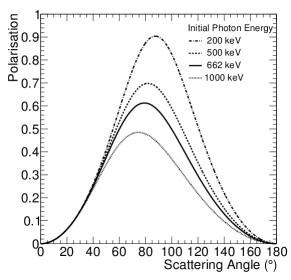
(a)

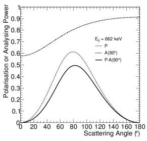
(b)

Figure 1: 1(a) Polarisation of photons following Compton scattering, as a function of the scattering angle. For photons of 662 keV a polarisation of 61.3% is obtained for a scattering angle of 80^∘. 1(b) Polarisation, analysing power at 90^∘, and measurable polarisation $PA(90^{\circ})$, for an initially inpolarised beam of photons with energy 662 keV scattered at various angles. The maximum measurable polarisation is 49.5% at 82.3^∘.

3 Experimental Arrangement

The experimental layout is shown in Figure 2(a), while a general view of the experiment is given in Figure 2(b). The apparatus consists of four NaI(Tl) scintillators, presented in Table 1. For the main experiment a collimated Caesium-137 source with an apperture of 3 mm is used, nominally at position “A”. Caesium-137 undergoes $\beta^{-}$ decay to Barium-137, and emits a 661.7 keV photon from the de-excitation of the daughter nucleus. The photon rate from the collimated source was of the order of a few tens of thousands per second.

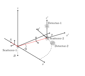
(a)

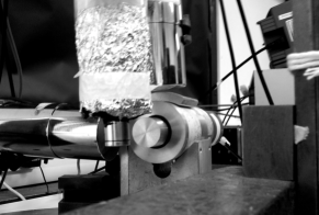
(b)

Figure 2: 2(a) Layout of the experimental set-up. 2(b) Photograph of the experimental set-up.

The photon, after leaving the source, impinges on Scatterer-1, at a distnace of 13 cm, and emerges at an angle of $80^{\circ}$, with an energy of 320 keV. Subsequently, it scatters off Scatterer-2, at a distance of 7.8 cm, and emerges at $90^{\circ}$ with 197 keV, and is detected in Detector-1 or Detector-2, which each lie at 7 cm from Scatterer-2. Detector-1 is in the plane perpendicular to the plane of the first scattering, while Detector-2 lies in the plane of the first scattering. Appropriate shielding was added using blocks of lead. The aim of the shielding was to obstruct direct line-of-sight from the source to Scatterer-2 and the detectors, as well as from Scatterer-1 to the detectors.

As estimated from a Geant4 simulation of the experiment, see Section 6, in the described experimental arrangement $40\%$ of the photons leaving the source interact in Scatterer-1, with $33\%$ of those interacting being fully absorbed. Approximately $1$ in $1000$ photons from the source arrive at Scatterer-2 having interacted with Scatterer-1, while $1$ in $100000$ photons from the source arrive at either Detector-1 or Detector-2. Of the photons observed in Detector-1 and Detector-2, 78.5% have undergone a single scattering in Scatterer-1, while 74.3% have scattered only once in Scatterer-2.

Table 1: The dimensions of the cylindrical NaI(Tl) scintillators used in the experiment, along with their measured energy resolution.

Name	Diameter	Length	Energy Resolution
	(in.)	(in.)	FWHM at 511 keV
Scatterer-1	0.75	1	8.3%
Scatterer-2	1	1	7.7%
Detector-1	2	2	7.0%
Detector-2	2	2	6.9%

4 Detector calibration and characterisation

The detectors were calibrated using photons of known energies from a variety of radioisotopes [13]: ⁶⁸Ge, ²⁴¹Am, and ^108mAg. Germanium-68 decays by electron capture to Gallium-68 which itself decays to Zinc-68 via $\beta^{+}$ decay. The annihilation of the positron releases two back-to-back 511 keV photons. Americium-241 disintegrates through $\alpha$ decay to Neptunium-237, which in turn emitts a 59.5 keV photon. Silver-108m undergoes electron capture to Palladium-108 and emitts, among others, a 433.9 keV $\gamma$-ray. In particular, Scatterer-1 was calibrated also using the 661.7 keV line of Caesium-137 to allow monitoring of the photo-absorption. Beyond energy calibration, these data have also been used to estimate the resolution of the detectors, through the full-width at half-maximum (FWHM) of the peaks in the obtained spectra. The timing of the various detectors was studied and synchronized using annihilation photons.

To avoid apparent asymmetries between the two detectors their efficiency was measured and compared. Annihilation photons from Germanium-68 were used in the coincidence technique: Detector-1 and Detector-2 were placed symmetrically about the source, and the detection of a photon in Detector-1 was used as the trigger signal to search for the other photon in Detector-2, and vice-versa. The efficiencies of the two detectors were found to be 28% and 26% respectively. Based on this a correction is applied to the data and a systematic uncertainty equal to the observed difference in efficiencies is assigned to the result.

5 Data acquisition

The pulses from Detector-1 and Detector-2 were amplified and each fed into a multi-channel analyser (MCA). In order to record signals which originated from scattering events, a logic signal was devised using the pulses from Scatterer-1 and Scatterer-2 and used to gate the two MCAs. The anode signals from Scatterer-1 and Scatterer-2 were fed into two timing single-channel analysers (TSCA) to select the energies and discard events not originating from the desired scattering pattern. A loose window was set for Scatterer-1, approximately, from 80 to 500 keV. A window from, approximately, 90 keV to 153 keV was set for Scatterer-2. The outputs of the single channel analysers were fed into a coincidence unit to produce a logic pulse. The diagram of the circuit is shown in Figure 3.

Figure 3: Block diagram of the read-out electronics of the experimental arrangement.

The single channel analyser windows were set by splitting the signal from the scatterer with one branch being fed to the timing single channel analyser as explained above, while the second branch was fed to a pre-amplifier and subsequently to a spectroscopy amplifier. The latter signal was appropriately delayed and fed to a multi-channel analyser while the former was used as a gate.

In the course of preparing the trigger signal, the background rates were also studied. Without the presence of coincidence requirements Detector-1 and Detector-2 recorded events at a rate of approximately $120\;{\rm s}^{-1}$. By requiring a singal from Scatterer-1, these rates were reduced by a factor 20, while requiring a signal from Scatterer-2 resulted in a reduction by a factor 1000, at which point about 50% of the observed events were in the signal region. If coincidence was required in both scatterers the detectors measured a rate of $0.032\;{\rm s}^{-1}$ and $0.073\;{\rm s}^{-1}$, respectively, with about 80% of the events in the signal region. To estimate the number of accidental coincidences, data were collected with the same setup but with an additional delay between the coincidence signal and the detector output.

6 Simulation of the Experiment

The experimental arrangement has been replicated using the Geant4 simulation toolkit [14], and the ratio $R$ has been obtained using the same selection requirements as in the data analysis. The experimental layout as implemented in simulation is shown in Figure 4.

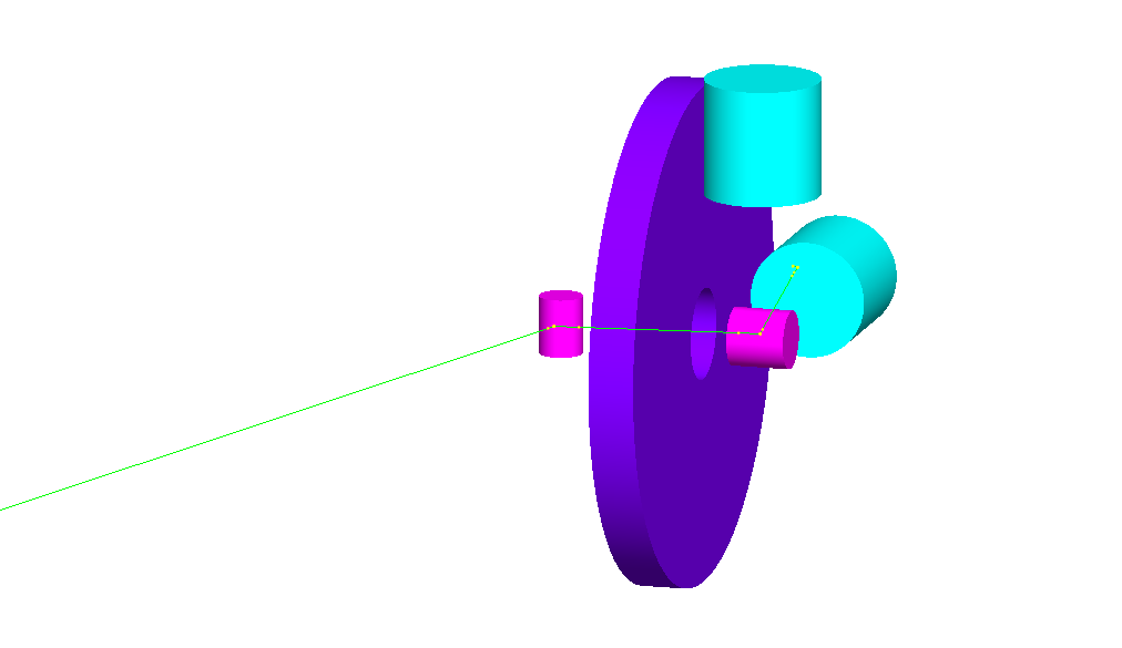
Figure 4: Experimental layout in simulation. The scatterers are shown in purple, the detectors in teal, and the shielding in violet. The photon path is shown in green.

To highlight the effects of photon polarisation and to check for apparent asymmetries of geometric origin, the simulation was also performed ignoring polarisation effects using the G4EmLivermore physics model. The estimated ratio was $R_{0}=\left(4\pm 2\right)\%$. As a result, geometry effects are found to induce a small asymmetry in the same direction as that induced by polarisation. The uncertainty on $R_{0}$ includes a systematic uncertainty due to potential mismatch between the energy thresholds applied in simulation and the experiment.

A direct experimental estimate of the apparent asymmetry due to geometry effects could be obtained by positioning a Germanium-68 source between Scatterer-1 and Scatterer-2. Using the signal in the two scatterers, in coincidence, as a gate and counting the number of photons impinging on Detector-1 and Detector-2 having undergone Compton scattering in Scatterer-2, an estimate of $R_{0}$ is obtained. This estimate neglects the effect of Scatterer-1 in the overall apparent asymmetry of the experimental arrangement.

7 Results

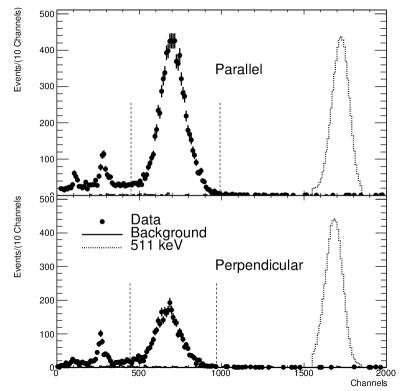
Figure 5: The obtained experimental yields of events for the detector Parallel (above) and Perpendicular (below) to the first scattering plane. The continuous histogram denotes the contribution from random coincidences. The vertical dashed lines denote the signal region, between 135 and 295 keV.

In Figure 5 the observed energy spectra from the two detectors are shown after 39-hours of data-taking. An asymmetry is readily observed. The peak at about 700 ADC channels is the photo-peak from the absorption of the scattered photons alongside the Compton continuum. At lower energies, the characteristic X-rays of lead from the shielding and of iodine are also observed. A positron annihilation photo-peak is overlaid to set the energy scale. From the number of counts in the area denoted by the vertical dashed lines in Figure 5, $R=\left(45\pm 3\right)\%$ is obtained, after the background from accidental coincidences is subtracted. The quoted uncertainty includes the statistical uncertainty of the measurement and the systematic uncertainty on the uniformity of response of the two detectors. From this, the polarisation of the photon beam after the first scattering is estimated to be $P=\left(56\pm 5\right)\%$, where a 5% relative uncertainty on the analysing power has been included.

These estimates do not account for the finite geometry effects discussed in the following section. If a correction is included for the observed apparent asymmetry observed in the simulation when no polarisation effects are included, the obtained ratio $R$ becomes $\left(42\pm 4\right)\%$ and the corresponding polarisation is $P=\left(52\pm 6\right)\%$, in agreement within uncertainties with the expectation.

As a cross-check, the experiment was repeated with a Caesium-137 source placed in position “B”, see Figure 2(a), effectively interchanging the roles of Detector-1 and Detector-2 as “Parallel” and “Perpendicular”. An asymmetry was observed, albeit less pronounced and with larger uncertainties due to the inappropriate shape of the two scatterers for this orientation, which resulted in a wide spread of scattering angles and a larger geometrical asymmetry then the nominal experiment.

8 Discussion

The experiment described allows for the observation of the effects of polarisation in Compton scattering, starting from an initially unpolarised source available in the undergradute physics laboratories. Measurements were carried out over the period of hours, a time interval appropriate for the undergraduate laboratory by allowing the experiment to run overnight or a day. It is noted that the choice of scattering angles probes the region where polarisation effects play the most important role, but also results to an experimental arrangement that is relatively insensitive to small deviations of the detectors from the nominal positions.

The accidental coincidences, signals uncorrelated to scattering events, in the experiment have been estimated by introducing an arbitrary delay between the trigger signal, and the read-out of the detectors. Nevertheless, in the obtained energy spectra contributions are observed that seem to originate in-time with the scattering events, but are inconsistent with the expected energy for the photons following the desired scattering path. These contributions are consistent with the K-lines of Lead, 88 keV, and Iodine, 33 keV. Their energy is low enough to not obscure the measurement of the fully absorbed scattered photons.

Two different approaches have been implemented to control any potential apparent asymmetry in the counting rates due to systematic effects. In the first one, the photo-peak efficiency of the two detectors is measured using a coincidence technique with annihilation photons, to demonstrate the consistency. The measurement was performed before and after data-taking. The second approach involves the repetition of the experiment after moving the source from position “A” to position “B”, effectively interchanging the role of the two detectors as parallel and perpendicular to the plane of first scattering. A possible extension of this measurement could involve the measurement of the ratio $R$ as a function of the angular separation of the planes of the second scattering. Furthermore, the experiment may be performed with one detector, instead of two, by moving the same detector between the two positions, ensuring the equality of response of the detectors. However, in the interest of time it was deemed useful to take data in parallel.

In the presented experimental arrangement both scatterers were “active”, that is they were read-out and contributed to the background rejection. Nevertheless, from the background studies performed it is demonstrated that replacing the first scatterer with a brass rod would still be a viable solution.

A few comments on the minimum instrumentation requirements for this experiment are in line. In the experiment standard off-the-shelf 2” and 1” NaI(Tl) detectors were used. As discussed earlier, one could consider using the same detector for both Detector-1 and Detector-2 by moving it between the two positions, at the expense of longer data collecting periods. Nevertheless, in this case the required electronic units are reduced: One less pre-amplifier, amplifier, high voltage bias supply, and multi-channel analyser. The smallest detector, Scatterer-1, was built in-house from a sealed NaI crystal and a photo-multiplier tube (PMT). Sealed crystals and PMTs are readily available from a number of sources. However, Scatterer-1 could be still replaced by a standard 1” detector, or by an inactive scatterer, such as a copper rod. In this latter case, the required electronic units are also reduced: One less pre-amplifier, amplifier, high voltage bias supply, single channel analyser channel, and no need for a coincidence unit. Finally, a standard set of laboratory sources is needed for the calibration of the detectors, while a strong Caesium-137 source was required for the main polarization measurement. For the final implementation in the teaching laboratory a collimated $5\;{\rm MBq}$ source was used, together with the required shielding.

9 Summary

An experiment suitable for the undergraduate physics laboratory that demonstrates the effect of polarisation in Compton scattering was presented. An initially unpolarised beam of photons that undergoes two subsequent scatterings is employed. A coincidence technique, along with appropriate shielding, suppresses adequately the background from accidental coincidences. Additional controls of the detectors’ efficiency and inversion of their position verify the observed effect and provides the opportunity for a discussion of systematic uncertainties and their role in measurements.

This exercise could provide an effective introduction to the role of photon polarisation in nuclear and particle physics, allow for a project-type laboratory course, and introduce the students in background estimation techniques, systematic checks, and advanced simulation techniques, usually not discussed in the undergraduate laboratory.

References

References

- [1] A. H. Compton, “A Quantum Theory of the Scattering of X-rays by Light Elements,” Phys. Rev., vol. 21, pp. 483–502, 1923.
- [2] A. A. Bartlett, “Compton effect: A simple laboratory experiment,” American Journal of Physics, vol. 32, no. 2, pp. 127–134, 1964.
- [3] A. A. Bartlett, J. H. Wilson, O. W. Lyle, C. V. Wells, and J. J. Kraushaar, “Compton effect: an experiment for the advanced laboratory,” American Journal of Physics, vol. 32, no. 2, pp. 135–142, 1964.
- [4] W. R. French, “Precision compton-effect experiment,” American Journal of Physics, vol. 33, no. 7, pp. 523–527, 1965.
- [5] M. Stamatelatos, “Compton scattering experiment,” American Journal of Physics, vol. 40, no. 12, pp. 1871–1872, 1972.
- [6] P. L. Jolivette and N. Rouze, “Compton scattering, the electron mass, and relativity: A laboratory experiment,” American Journal of Physics, vol. 62, no. 3, pp. 266–271, 1994.
- [7] S. A. Hieronymus, L. L. Lundquist, and D. A. Cornell, “Application of high-purity germanium (hpge) detector to advanced laboratory experiment on the compton effect,” American Journal of Physics, vol. 66, no. 9, pp. 836–836, 1998.
- [8] A. Wightman, “Note on polarization effects in compton scattering,” Phys. Rev., vol. 74, pp. 1813–1817, Dec 1948.
- [9] E. Rodgers, “Polarization of hard x-rays,” Phys. Rev., vol. 50, pp. 875–878, Nov 1936.
- [10] J. I. Hoover, W. R. Faust, and C. F. Dohne, “Polarization of scattered quanta,” Phys. Rev., vol. 85, pp. 58–59, Jan 1952.
- [11] J. G. Hudson, “Polarization of compton-scattered gamma rays,” honors thesis, Western Michigan University, 1968.
- [12] W. Heitler, The quantum theory of radiation. The address: Oxford University Press, 2 ed., 1944.
- [13] A. Sonzogni, “Nndc chart of nuclides,” in International Conference on Nuclear Data for Science and Technology, pp. 105–106, EDP Sciences, 2007.
- [14] S. Agostinelli et al., “GEANT4: A Simulation toolkit,” Nucl. Instrum. Meth., vol. A506, pp. 250–303, 2003.