Semi-automated Signal Surveying Using Smartphones and Floorplans

Abstract

Location fingerprinting locates devices based on pattern matching signal observations to a pre-defined signal map. This paper introduces a technique to enable fast signal map creation given a dedicated surveyor with a smartphone and floorplan. Our technique (PFSurvey) uses accelerometer, gyroscope and magnetometer data to estimate the surveyor’s trajectory post-hoc using Simultaneous Localisation and Mapping and particle filtering to incorporate a building floorplan. We demonstrate conventional methods can fail to recover the survey path robustly and determine the room unambiguously. To counter this we use a novel loop closure detection method based on magnetic field signals and propose to incorporate the magnetic loop closures and straight-line constraints into the filtering process to ensure robust trajectory recovery. We show this allows room ambiguities to be resolved.

An entire building can be surveyed by the proposed system in minutes rather than days. We evaluate in a large office space and compare to state-of-the-art approaches. We achieve trajectories within 1.1 m of the ground truth 90% of the time. Output signal maps well approximate those built from conventional, laborious manual survey. We also demonstrate that the signal maps built by PFSurvey provide similar or even better positioning performance than the manual signal maps.

1 Introduction

The advent of personal computing devices has brought with it an increased demand for location-based services. These services have been powered primarily by Global Navigation Satellite Systems such as GPS due to their wide availability and high accuracy. However, these systems can only provide location outdoors. Within buildings—where people spend the majority of their time—ubiquitous location remains elusive. Many research prototypes have been developed but wide deployments are typically hindered by the need for custom infrastructure.

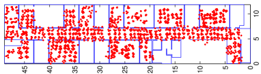
(a) An example grid-based manual survey.

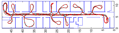
(b) An example path survey

Figure 1: Manual survey vs path survey

The most successful systems in terms of adoption are based on repurposing existing infrastructure, often exploiting pervasive WiFi signals. Due to the complex propagation of radio indoors, the empirical fingerprinting location technique has dominated. This involves two stages: an offline signal survey at regular points throughout the space of interest (e.g. Figure 1(a)) to collect signal strength samples labelled with location information; then an online positioning phase where the labelled samples are used to create a radio map, and radio measurements observed at the mobile device are pattern-matched to this map. Although this can achieve good positioning results the offline survey is typically laborious. Coupled with the need for regular resurveys due to environment changes, this has limited the scalability (and general availability) of fingerprinting. To illustrate this point, mapping 450,000m² of the COEX complex in Seoul, Korea is reported to have required 15 surveyors and taken two weeks [18].

Some researchers have advocated crowdsourcing the signal survey process. In some sense, the survey is then ‘free’: a survey point is created by any device that knows its location (or can be subsequently located) and is willing to report its current observations. This is a highly scalable concept, but there are a number of practical issues that have prevented its wide use to date:

1. The crowdsourced data collection is battery-intensive. It usually requires all of the inertial sensors to be on alongside continuous WiFi scanning and other sensing. Typical users are reluctant to run sensors they are not directly using since they reduce battery life; heat up the phone; and interfere with normal usage (e.g. repeated WiFi scanning adversely impacts the WiFi performance).

2. Map quality can vary dramatically according to the volume and quality of the crowdsourced data in a specific space. This results in inconsistent location accuracy, which is difficult for location-aware applications to handle. Furthermore, the places that are less interesting to most people (so the volume and quality of the crowdsourced data are low) could be important for others. A good example is the areas such as toilets for disabled people. This inconsistency harms the user experience of these people who needs special care.

3. Security and privacy are potentially at risk. Malicious users could contrive to adapt the map to their advantage, and privacy is at risk unless the data are carefully anonymised (which may be difficult given that devices must be individually profiled for best results).

4. Device heterogeneity makes it difficult to combine crowdsourced measurements. A number of previous works have reported significant differences in the signal strength measurements made on one phone model to those made on another in the same context [23].

5. Even the same device can record a different fingerprint at the same location according to its context. For example, being carried in-hand vs in-pocket vs in-bag vs within a dense crowd.

This paper investigates a different approach for the offline signal survey. We retain the notion of a dedicated surveyor (i.e. a user who is willing to follow specific guidelines to explicitly collect the fingerprint data needed), and focus instead on how to make their job much easier. The core idea is to collect survey data along trajectories rather than at discrete grid points. We advocate that if the trajectory can be accurately embedded in a building’s frame of reference, any signals measured along the path are survey points (i.e. a triple of {time, signal strength, location}) that contribute to a larger path survey as illustrated in Figure 1(b). The black line represents the surveyor’s trajectory; the red points are the measurement points. Then the signal survey is done simply by finishing a trajectory (or trajectories) that explore a given space comprehensively.

By removing the laborious manual survey and advocating the use of a dedicated surveyor, we enable efficient signal surveying which has the following advantages over crowdsourcing:

1. Power consumption is no longer a major concern because we do not require the user to contribute to the signal survey. A survey walk finishes much quicker than a manual survey (minutes vs. hours).

2. A dedicated surveyor can guarantee the space has been surveyed comprehensively to achieve consistent positioning accuracy.

3. Security and privacy are protected since no user data transmission is needed in the signal survey.

4. The problem of device heterogeneity could be alleviated because we can at least guarantee that only a single device is used to conduct one signal survey. To generalise the signal samples collected by one device to different kinds of device, some techniques like [20] could be used.

5. For the problem of different phone positions, the dedicated surveyor can keep the phone position constant. This has the additional benefit that the grip can be chosen to make the step detection problem simpler.  [4].

In terms of cost, our proposed survey method requires a dedicated surveyor to do the survey task. But our method enables the survey to be done on a regular basis in extremely low cost because we are able to simplify the survey to a simple walk that passes within a few metres of anywhere that positioning is required. Surveying a typical office space takes only minutes and may even be carried out by security personnel or cleaning staff (both of which are expected to visit all of the building regularly).

However, this approach is challenging in practice: high quality trajectory estimation is difficult and accurate trajectory embedding is rarely possible. To solve this, we present PFSurvey and make the following contributions in this paper:

• We show how traditional particle filtering techniques can fail to recover the survey path robustly.

• We propose the PFSurvey system that uses smartphone accelerometer, gyroscope and magnetometer data to estimate a dedicated surveyor’s trajectory post-hoc using Simultaneous Localisation and Mapping (SLAM) techniques and particle filtering to incorporate a building floorplan.

• We propose a novel loop closure detection method based on magnetic field signals and show how magnetic loop closures and straight-line constraints can be incorporated into the filtering process to ensure robust trajectory recovery.

Our focus is on the offline signal survey, the purpose of which is to collect signal strength samples and label them with location information. Our goal is to reduce the efforts of a signal survey by allowing them to simply walk around the environment (a path survey). The subsequent online positioning phase, which uses the data to estimate position, is out of the scope of this work, although we use a straw-man implementation to illustrate our results. A more rigorous evaluation can be found in [14].

1.1 A Dedicated Surveyor

We emphasise that we assume a dedicated surveyor in this work. This is motivated by our belief that Pedestrian Dead reckoning (PDR) algorithms are not sufficiently mature to robustly estimate the trajectories of arbitrary multi-purpose devices. Assuming a dedicated surveyor affords us a number of advantages:

• the surveyor will carry the smartphone consistently; We require the surveyor holds the phone flat in front of the human body as if navigation. This increases the success rate of PDR algorithms, which is the very first step of the proposed system.

• the surveyor will cover the area comprehensively following best-practice guidelines. This ensures the quality of the signal maps being built.

• a start position can be manually specified. This is not mandatory, but significantly reduces the computational complexity.

We have previously described some survey guidelines to give good results [14], summarised here for convenience:

• The survey path should visit each room and pass within 1–2 m of wherever positioning is required.

• The surveyor should repeat some parts of the path to increase the signal sampling density (particularly important for WiFi).

• Each path should be traversed in both directions wherever possible.

Many public buildings have security or building management personnel who regularly walk through them. These people offer an ideal opportunity to perform regular surveys. Note that because our approach does not require a ‘live’ location estimate, we can post-process the data using greater computational resources.

By quantitative evaluation, we demonstrate that our system achieves good accuracy and efficiency in trajectory recovery. We also demonstrate that the signal maps built by our system well approximate the signal maps built by a more costly manual survey and provide similar or even better positioning performance.

2 Related Work

Indoor location. Indoor location is an active research field—comprehensive surveys of the many prototypes and techniques can be found in [28, 2, 25, 17]. In this work we seek to produce radio maps from a (possibly jointly) estimated trajectory.

Radio maps. The idea of a radio map for location stems from the RADAR system [3], which was extended by the Horus system [37] and many others [19]. Most of these systems assume an offline manual survey where a surveyor measures the signal at each point on a fine grid covering the indoor area. This is a difficult task, partly due to the lengthy and laborious nature of the work and partly because it is difficult to ensure the measuring device is precisely at a given grid point.

Inertial sensors and Pedestrian Dead Reckoning. Estimating the trajectory of a pedestrian without dedicated infrastructure has been achieved in a number of ways. The starting point is some form of step detection based on the inertial sensors, where a step is characterised with a length and (possibly change of) heading. This can be achieved very accurately using foot-mounted sensors [33], or more coarsely with unconstrained devices [4]. Accumulating the step vectors leads to a raw PDR trajectory that is prone to drift.

This drift can be constrained using extrinsic information, particularly floorplans. A particle filter is typically used to ensure the trajectory remains consistent with the floorplan. Systems such as [33, 26] provide instantaneous location estimates—i.e. at time $t=T$ they sample the probability distribution for the current position based on all measurements and state for $0<t<T$. The position estimate is usually taken as the weighted mean of the samples.

Post-hoc trajectory estimation. In this work we do not require instantaneous location estimation as the data arrive but rather a best estimate of the trajectory post-hoc. Thus at time $t=T$ we want to estimate the probability distribution given the events at all epochs, even the ‘future’ ones ($t>T$). Essentially, knowing where we are now may allow a better estimate of where we were, particularly if we were uncertain at the time (e.g. a multi-modal distribution). Particle smoother algorithms are commonly used to provide the best post-hoc estimates. For example Fixed Lag Smoothing (FL) [24], Forward Filter Backward Smoothing (FFBS) [7] and Forward Filter Backward Simulation (FFBSi) [16]. These involve retaining the particle distributions at each epoch (which can be costly in terms of space) and reprocessing at various stages (which can be computationally costly)

A simpler but less formally correct approach was described anonymously in [8] (DP-SLAM)—we refer to it as particle pruning. An ancestor tree for each particle is retained as before. However, when a particle is not resampled we walk up its ancestor branch, removing any parent particles in previous epochs that have no other child (‘pruning’). At the end of the filter, the position at each epoch is computed as the weighted mean of the remaining particles for that epoch. The pruning approach is less resource-intensive but needs a large number of particles to ensure older epochs do not suffer particle depletion.

SLAM. An alternative post-hoc approach is to use external spatially-variant signals (possibly even those we wish to map) to enable Simultaneous Localisation and Mapping (SLAM). The core idea is to search the external observations for evidence of loops in the trajectory (when the external observations return to values recorded earlier in the trajectory). These form loop closures that are used to constrain the post-hoc trajectory estimate. The SLAM algorithms are either graph-based (e.g. GraphSLAM [21]) or use particle filters (e.g DP-SLAM [8] and FastSLAM [29]). They have been used when a floorplan was unavailable, giving unanchored trajectories. Section 3 shows that these unanchored trajectories actually have limited use since they cannot easily be mapped back to meaningful features (e.g. specific rooms). So this SLAM method is optimal only when a floor plan is not available.

Crowdsourcing. Crowdsourced radio map systems often make use of a variety of the techniques just listed. Zee [31] fuses user traces to a floor plan using a particle filter and WiFi to help locate later traces. UnLoc [32] locates traces to a floorplan via landmarks. WILL [36] clusters fingerprints collected along traces into “virtual rooms”, and then maps virtual rooms to physical rooms on the floor plan automatically by the proposed subsection mapping method (SSMM). LiFS [35] maps a high dimensional fingerprint space formed by RSS fingerprints and traces to physical space (floor plan). Chai et al. [5] collect fingerprints labelled with location information on sparse sample points to generate an initial map, and then locates traces to the floor plan using this map and then iteratively improves the map. EZ [6] and LARM [30] try to model the signal strength distribution using learning-based methods, but they still need some fingerprints labelled with location information. UCMA [22] is also a learning-based crowdsourcing system but requires no labelled fingerprints and no inertial data. It proposes a method that integrates a memetic algorithm and a segmental k-means algorithm in a hybrid global-local optimisation scheme to locate unlabelled fingerprints to the floor plan. WiFi-SLAM [9] models the signal strength distribution and simultaneously recovers the trajectories. It is based on the assumption of dense AP deployment and still needs some labelled data to train the initial values for some model parameters. WiFi GraphSLAM [21] also recovers and corrects user traces using WiFi signals but it relaxes the assumption of dense AP deployment by incorporating inertial sensors.

Clearly many of these crowdsourcing systems also require a trajectory-recovery component like the one used in this work. However, trajectory recovery is rarely straight-forward and/or accurate enough in these systems. This is why they need to work with other components together to map the signal environment. More complicated survey trajectories like those shown in Figure 2(a), 4(a) and 4(d) are very challenging for such systems. This is especially true for those based on signal propagation models like WiFi-SLAM [9] and WiFi GraphSLAM [21]. Furthermore, they suffer from the general problems outlined in the Introduction above.

In contrast our proposed system recovers the trajectory explicitly and accurately, and is much simpler and more practical to use. It does not rely on any signal propagation model and reduces the efforts of the signal survey to a simple walk around the environment.

3 Path Surveys

Use PDR-traj as input	Use SLAM-traj as input
Input No smoothing Pruning FL FFBSm FFBSi Particle Cloud	Input Non-Smoothed Pruning FL FFBSm FFBSi Particle Cloud

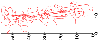
(a) PDR-traj

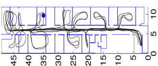
(b)

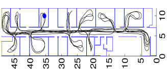
(c)

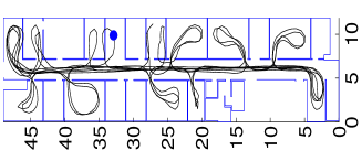
(d)

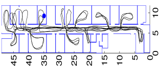
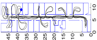
(e)

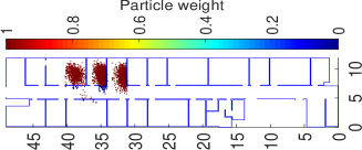
(f)

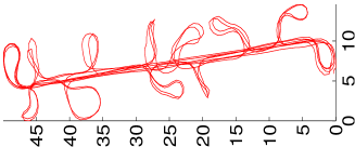
(g) SLAM-traj

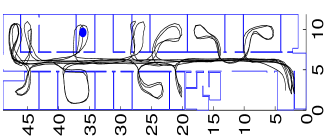
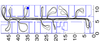
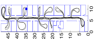
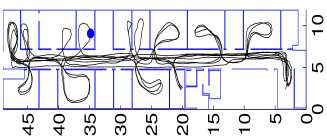
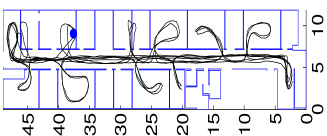
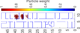
(h)

Figure 2: Example outputs of the conventional particle filter plus smoother approach. The ground truth trajectory is shown in Figure 1(b). These results show that state-of-the-art techniques failed in giving robust trajectory estimation.

We consider any PDR-based system that maps a spatially-variant quantity using trajectories rather then grid point measurements to be a path survey. The primary goal of this work is to produce the best trajectory estimate consistent with (and anchored to) a floorplan. This section evaluates state-of-the-art techniques that could potentially enable path survey. We try different combinations of various techniques and show why they fail.

The simplest solution is to feed the raw PDR trajectory (herein referred to as PDR-traj) into a wall-sensitive particle filter and then use a particle smoother to recover the optimal trajectory. The left column of Figure 2 illustrates this case. The raw PDR-traj path exhibits typical drift issues seen when walking a path such as the ground truth (Figure 1(b), obtained using a high accuracy ultrasonic positioning system [1]). The error is sufficiently high that various smoothers give significantly different trajectory results (Figures 2(b)–2(e)). Moreover, the trajectories are not truly consistent with the floorplan, since they cross walls (or enter wrong rooms) at various points. The explanation for this can be seen in Figure 2(f), which shows an instantaneous particle distribution corresponding to the point marked with a blue dot in the preceding images. The high PDR uncertainty results in multi-modal distributions spanning multiple rooms. The position estimate is a weighted average of these particles and so can cross walls. This room ambiguity is very serious for a path survey: a small perturbation to any of these systems could easily result in signal data being assigned to the incorrect room and the subsequent radio map containing serious errors.

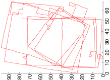
(a) Raw PDR result.

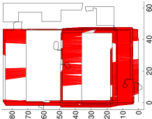
(b) Pre-processed PDR result (black trajectory) with loop closures (dense red lines).

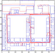
(c) SLAM result plotted on floor plan.

Figure 3: Example scaling errors from SLAM without a floorplan. (a) the input PDR-traj. (a) the PDR-traj was pre-processed by straight line filter and the loop closures were detected. (c) the SLAM result after manual alignment to the floorplan.

To reduce the chance of multi-modal distributions we can preprocess the PDR trajectory to correct the drift based on external observations. For example we have previously demonstrated a GraphSLAM-based system that does this by applying loop closure constraints when a floorplan is unavailable [13]. Figure 3(b) shows the loop closures on a typical (pre-processed) PDR trajectory. These loop closures were detected by a window-based searching scheme that matches similar magnetic sequences recorded along the walking path. Based on these detected loop closures, the GraphSLAM system could then correct the PDR drift to a large extent as showed in Figure 3(c) (the red trajectory). However, the optimised trajectory may have incorrect scale and might violate the environmental constraints. Figure 3(c) shows the SLAM results on top of the floorplan (manually aligned). We observe that the path crosses the walls and different parts of the trajectory have different scaling errors. The reason for this is that the loop closures only give information about the spatial relationships between the surveyor’s positions at different time points/steps, but not any information about the environmental constraints (floorplan). So a pure loop closure-based SLAM system is not adequate to correctly recover the survey path.

A natural adaptation would be to take the low-drift (compared to raw PDR trajectory) SLAM-corrected trajectory (herein referred to as SLAM-traj) and pass that through a floorplan-sensitive particle filter and estimate the trajectory via a particle smoother or pruning. The right column of Figure 2 illustrates this idea. Compared to PDR-traj (with both heading and scaling errors) the SLAM-traj has much lower heading noise as can be seen in Figure 2(g). However, the scale errors persist and we typically find that the final result is only marginally better. For these runs we see that only the FL smoother was able to correctly recover the path (in fact part of the trajectory still penetrates walls if observed carefully, but the error is negligible). However, closer inspection of the particles at the position marked with a blue dot in the smoother outputs shows that the distribution was still multi-modal (Figures 2(h)). This is more obvious for longer walks such as those in Figure 4, where the FL smoother produced poor results (highlighted in magenta) when faced with multi-modal distributions.

	Input (PDR-traj)	FL	Particle Cloud
Path-2
Path-3

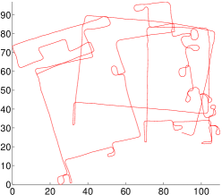
(a)

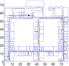
(b)

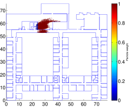
(c)

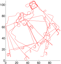
(d)

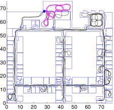
(e)

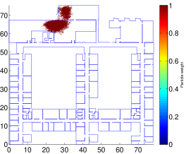
(f)

Figure 4: Example outputs of the conventional particle filter plus smoother approach on longer walks.

4 PFSurvey Design

We believe that a fundamental reason for the ambiguities in the PDR-traj-based filtering results discussed in Section 3 is the lack of sufficient constraints to distribute weights reasonably over the particles. Please note that a particle represents a hypothesis about the 2D pose (coordinates x, y and orientation) of the surveyor. Each particle is associated with a weight represents the possibility of this hypothesis to be true. During the filtering process, particles with larger weights are more likely to be selected and survive than those with lower weights. The wall-sensitive particle filter and smoother kills all particles violating environmental constraints and gives all the surviving particles the same weight, e.g., a weight of $\frac{1}{N}$ for number of surviving particles, $N$. Thus, all surviving particles have equal probability of being re-sampled no matter how likely it is they hold the true hypothesis of the system state. For the results in Figure 2 and 4, the particle clusters spread in the wrong locations have similar weight sums with the particle clusters in the correct place. This causes ambiguities and incorrectness in the final result. While loop closures can assist by limiting the drift (i.e. keeping the particle clouds small), the common techniques used to process them cannot incorporate floorplan constraints.

PFSurvey attempts to use both the floorplan and loop closures simultaneously to produce a more robust and accurate trajectory estimate. The core fusion process is a particle filter, but a series of pre-processing steps are necessary to create suitable loop closures. The system architecture is illustrated in Figure 5 and contains a series of components:

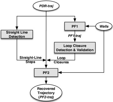
Figure 5: The work flow of the proposed trajectory recovery system.

Particle Filter 1 (PF1). This step takes the PDR-traj as input, runs a wall-constraints-only particle filter to improve the topology of PDR-traj. This is to bound the PDR drift using the floor plan to reduce heading errors. We denote the resultant trajectory of this step as PF1-traj.

Straight line constraints. We typically build our environments to be rectilinear and tend to move in straight lines. However, in the PDR results straight line steps often bend due to bias errors from the gyroscopes. We use a simple threshold-based method to identify probable straight-line steps in the PDR results. Then we weight particles in PF2 according to how well their headings match the orientations suggested by the environments (rooms or corridors).

Loop closure detection & validation. This step detects and validates loop closures using the partially-corrected PF1-traj. Without the initial PF1 pass, robustly identifying true loop closures is often all but impossible. We provide details of our detection and validation scheme in Section 4.3.

Particle Filter 2 (PF2). This step adopts a customised particle filter to produce a survey trajectory consistent with the environment. It uses the wall, straight-line and loop closure constraints to weight the particles using PDR-traj as input. We denote the resultant trajectory of this step as PF2-traj, which is the final output. We now consider each of these components in more detail.

4.1 PF1

PF1 takes the noisy PDR-traj as input and aims to correct large heading errors in the raw PDR-traj using the floorplan. PF1 is based on previous work using particle filters and a foot-mounted IMU [33]. We adapt it to use 2D step vectors from handheld smartphones, which are significantly more noisy than the inputs used in the original work. In particular the step length is unobservable. We represent a step event as $m_{i}=(l,\delta\theta_{i})$, where $l$ is a fixed step length of 0.75 m and $\delta\theta_{i}$ is the heading change of the surveyor during this step as estimated by the gyroscope. The error models for these two components are assumed to be independent and Gaussian:

$$\begin{split}e_{l}&\sim\mathcal{N}(0,\sigma_{l}^{2})\\ e_{\delta\theta}&\sim\mathcal{N}(0,\sigma_{\delta\theta}^{2})\end{split}$$ (1)

Considering the sensor characteristics of modern smartphone, we set the uncertainty in the heading change $\sigma_{\delta\theta}=0.5^{\circ}$ and the step length uncertainty to $\sigma_{l}=\lambda l$. We set $\lambda=0.5$. The large uncertainties mean we are not sensitive to the parameter values, at a small cost of additional computation resource.

PF1 (and indeed PF2) implement KLD adaptive resampling [11, 33] to dynamically vary the number of particles appropriately at each step and constrain the computation requirements without impacting the result quality. KLD-sampling adapts the particle number based on the uncertainties of the system and some pre-defined parameters. Particles from one generation are segmented into bins based on their location and the number of occupied bins, $k$, used to determine the number of particles in the new generation. In the discussion that follows we briefly justify our other KLD parameters, full descriptions of which can be found in [11, 33, 34]. We determined the KLD parameters as follows:

1. The bin sizes $\Delta_{x}$, $\Delta_{y}$ and $\Delta_{\theta}$. Smaller bin sizes mean more bins occupied by the particle cloud hence cause more particles to be sampled, giving generally better performance. Since PF1 is solving the standard wall-constraints-only problem, we adopt parameters that have been shown to work well for that task [34]: $\Delta_{x}=\Delta_{y}=2.0~{}m$ and $\Delta_{\theta}=30^{\circ}$.

2. The bounding parameters $\delta$ and $\epsilon$. KLD-sampling ensures that the error introduced by the sample-based approximation of the posterior distribution is below a specified threshold $\epsilon$ with probability $\delta$. We set $\delta=0.01$ as in [34, 11, 12]. We compute a value for $\epsilon$ such that the required number of particles is 300 for small $k$. Using the following standard approximation,

   $$n_{req}\approx\frac{k-1}{2\epsilon}(1-\frac{2}{9(k-1)}+\sqrt{\frac{2}{9(k-1)}}z_{1-\delta})^{3},$$ (2)

   where $z_{1-\delta}$ is the upper $1-\delta$ quantile of the standard normal distribution, we find $\epsilon=0.0109238$ for $n_{req}=300$ and $k=2$.

3. The minimum number of particles $n_{min}$ required at each step. KLD resamples particles until the number is greater than both $n_{req}$ (Equation 2) and $n_{min}$. The latter is important since small $n_{min}$ is risky: when the particle cloud has converged to just a few bins, the particles may all fall into a subset of bins that does not contain the true state simply by chance. This causes $n_{req}$ to be too small. In this case, if $n_{min}$ is not large enough, insufficient particles will be sampled and the true state may be lost. To avoid this we set $n_{min}$ to be the number required by KLD sampling when the particle cloud has converged to an area with size $\Delta_{x}*\Delta_{y}$ in the $x-y$ plane and all the bins in the $\theta$-dimension are occupied, i.e.,

   $$n_{min}=n_{req}\left(k=\frac{2\pi}{\Delta_{\theta}}\right)$$ (3)

   This gives $n_{min}=504$.

With these parameters PF1 typically uses hundreds of particles and can finish within 3$\sim$5 seconds for a 10-minute survey walk (about 950 steps), assuming the surveyor provides the initial room or corridor (a reasonable expectation for a dedicated surveyor). To generate an output path we apply the pruning smoother. Since we do not care about room ambiguities in the output of PF1, it offers the least resource-intensive solution. Other smoothers could be applied but would come at additional complexity for no particular accuracy gain.

4.2 Straight Line Filter

This component first identifies candidates for straight-line steps from the original PDR-traj. It uses a simple threshold-based method: we identify consecutive steps where the turning angle is less than t^∘ to form candidate straight line steps. Considering the gyro bias is relatively low and the surveyor is required to carry the smartphone consistently (holding the phone flat in front of the human body as if navigation), we set $t=5$ and found this value works well in our case. Where there are $l$ or more candidates in a row, we assert that they are all straight line steps. The remaining candidates are discarded. To ensure the robustness of the straight line filter, the value of $l$ should not be too small because this may cause many false positive straight-line movements being detected. And $l$ cannot be very large otherwise it would exceed the length of the longest straight corridor in the environment. By tests we found setting $l=10$ is suitable for most indoor environments. The evaluation and discussion of this are given in Section 5.1.

4.3 Loop Closure Detection and Validation

For optimal results, this component must detect a sufficient number of true-positive loops in the trajectory without also detecting many false-positive loops. In principle loops can be detected directly from the PDR-traj (e.g. by looking for the same external signal values at different times). This leads to a large number of false positive closures since signals can reasonably adopt the same values at different spatial locations. We seek instead to find loop closures that link parts of the estimated trajectory that are already spatially close. This is the motivation for the PF1: it corrects the large heading errors that result in even true loop closures being spatially far apart (and hence difficult to distinguish from false positive closures).

We have developed closure detection algorithms based on monitoring sequences of magnetic readings [13]. Magnetic signals are ideally suited to the task: they have strong variance over space, which is mainly due to the steel shells of most modern buildings; they are temporally stable indoors (standard variance is typically within $0.001$ Earth field strength [27]); the sensors are low power with frequent updates. We have not found them to be a good signal to map for subsequent localisation because they are very easily influenced by small changes to the environment and hence transient in nature. But during a single dedicated survey walk lasting minutes, it is safely to assume that the disturbance like electronic devices is minimal, i.e. the signal is stable. The technique proceeds as follows:

Segment Pair		Maximum Segment Pair 1		Maximum Segment Pair 2

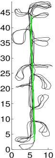
(a) Segment A.

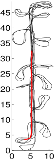
(b) Segment B.

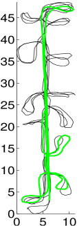
(c) Segment A.

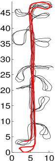
(d) Segment B.

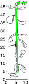
(e) Segment A.

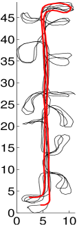
(f) Segment B.

Figure 6: Examples of PF1-traj, segment pair and maximum segment pair

	Maximum Segment Pair 1	Maximum Segment Pair 2
Sequence of Magnetic Magnitude
Warping Path
Magnetic Loop Closures
PDR Loop Closures

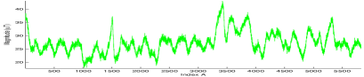
(a) Segment A.

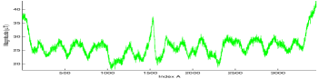
(b) Segment A.

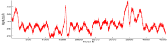
(c) Segment B.

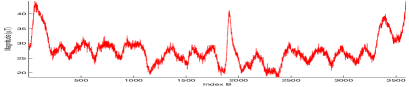
(d) Segment B.

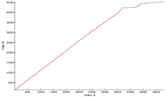
(e)

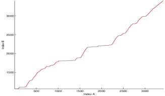
(f)

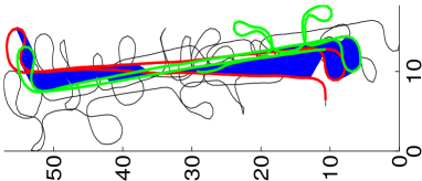
(g)

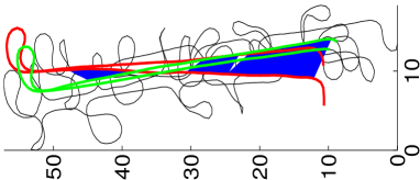
(h)

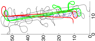
(i)

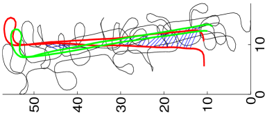
(j)

Figure 7: Loop closure detection/validation examples for two maximum segment pairs in Figure 6.

1. Generate PF1-traj as in Section 4.1.

2. Maximum Segment Pair (MSP) search . A segment is any consecutive part of the position sequence, $s=\{i_{s}:i_{e}\}$, where $i_{s}$ and $i_{e}$ are the start and end indices in PF1-traj. We process PF1-traj to find segment pairs, $(s_{1},s_{2})$, which are spatially close and hence candidates for being loop closures (we verify this latter property in the next step).

   Clearly an arbitrary segment could be contained within another (e.g $s_{j}=\{i_{4},i_{6}\}$ is contained by the longer $s_{k}=\{i_{4},i_{9}\}$). To avoid duplicating effort in subsequent steps we wish to find the Maximum Segment Pairs (MSPs), which are simply the segment pairs containing the longest segments possible without their elements violating the spatial proximity rule.

   Examples are given in Figure 6. The black trajectory is the output of PF1 when input with the PDR trajectory shown in Figure 2(a). Three pairs are shown: one an arbitrary segment pair; and the other two maximum segment pairs. In each case one part of the pair is shown in green, the other in red. The arbitrary segment pair is not a maximum segment pair because it is contained by maximum segment pair 1.

   Our algorithm for finding the MSPs is described briefly here for the situation illustrated in Figure 8, which shows a short 9-step trajectory. We first visit each index of PF1-traj, linking it with all other indices that lie within a distance, $R$ (shown as green circles for the first few steps). We then make a sequential pass over PF1-traj, checking the linked indices to see if they are increasing (or decreasing) in sequence, indicating they run in parallel. In the example, we move from 0 to 3 and simultaneously observe 8,7,6,6,5 (we observe 6 twice due to variance in the step length causing it to be in range of multiple earlier steps). Thus we find an MSP $\{\{0:3\},\{8:5\}\}$.

   

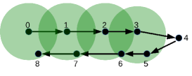
   Figure 8: Determining MSPs

   To set the value for $R$, please note that the drifts in PF1-traj have been bounded by the floor plan. Because the average width of a room/corridor on the floor plan used here is about $2\sim 3$ metres, the drifts in PF1-traj are bounded within this range. Therefore we conservatively set $R$ to 3 metres. This value was found to work well for all the cases tested.

3. Sequence-based magnetic loop closure detection. Having found an MSP, we must then determine the loop closures it contains. We do so using the magnetic signal strength. We associate each magnetic measurement with a PF1-traj position using time interpolation.

   Figure 7(a) and 7(c), Figure 7(b) and 7(d) are typical examples of magnetic signals in MSPs. The similarities between the magnetic sequences (waveforms) can be seen clearly from these figures. The intuition is that if we can match parts of Segment A to Segment B, we can assert loop closures between physical points on these two path segments. We use Open-Begin-End Dynamic Time Warping (OBE-DTW) with an ‘asymmetric’ step pattern [15] to get point-to-point correspondences (loop closures) between segments. OBE-DTW compresses or stretches the time series to create a ‘warping path’ between the segments. A point $(i,j)$ on the warping path means the $i^{th}$ element of $M_{1}$ matches to the $j^{th}$ element of $M_{2}$ (Figure 7(e) and Figure 7(f)). A horizontal segment in the warping path means DTW has either stretched one of the signals to fit (accounting for a speed difference) or mapped a chunk of the segment to one value on the the other segment since that chunk does not match anything. The latter situation leads to false positive closures.

   We therefore filter the warping path, splitting the segments into sub-segments at each horizontal part of the warping path. For example, several sub-segments are created from Figure 7(e) and Figure 7(f) respectively (all shown in red). The sub-segments are carried forward as possible matchings (sequences of loop closures).

4. Closure validation. The closure detection algorithm produces a large number of potential closures based solely on the magnetic observations. We apply a series of spatial criteria to reject matched subsequences, $N$ and $M$, that we are not confident in. The criteria are based on empirical constants chosen to be aggressive in culling closures—we would rather have a few true positive closures than a lot of true positives mixed with false positives. As such the constant values are not particularly sensitive.

   • Either $length(N)$ or $length(M)$ must be larger than 2.5 m (about 3$\sim$4 human steps). We expect that at least 3$\sim$4 steps are contained in a valid loop closure sequence.

   • Assume $length(N)>length(M)$, then the $\frac{length(N)}{length(M)}$ must be less than 2.0. This is to ensure the magnetic time series are not over compressed (stretched) because speed changes are not expected to be great.

   • $M$ and $N$ must be physically close. Because PF1 has corrected the trajectory to within some scaling errors we do not trust any instances where $M$ and $N$ are not physically close. To assess this we compute the mean spatial distance between the matched points of $M$ and $N$ on PF1-traj, $D_{mean}$. We require this value empirically to within $3.0$ m, which is the upper limit of the drifts in PF1-traj as described earlier in this section.

   • Additionally we expect the shapes of the two segments to be similar. To capture this we use the variance of the distances between the matched points, $D_{var}$. We set this value empirically to lie within 1.0 m².

5. Closure step mapping. We now have loop closures between magnetic measurement points on the survey path (Figures 7(g) and 7(h)). The closures are very dense due to the high sampling rate of the magnetic signal. However, we only need closures at matching points in the gait cycle. This thinning can be done using time interpolation for the part of path segments that covered by the dense magnetic loop closures—e.g. Figure 7(i) and 7(j). Now the loop closures only connect the end points of human steps to corresponding points on the survey path (we call them the PDR loop closures), which are far sparser than the original magnetic loop closures.

4.4 PF2

The previous stages can be seen as pre-processing for this major pass with a particle filter. The filter is an extended version of PF1 where we seek higher accuracy output. To that end we adapt the KLD resampling parameters of PF1 such that $\Delta_{x}=\Delta_{y}=0.5~{}m$, and $\Delta_{\theta}=1^{\circ}$. The new value of $n_{min}$ is then 16433. PF2 must incorporate the straight line and loop closure constraints at the particle reweighting stage. The full reweighting procedure for particle $p_{i,t}$ incorporating step $s_{t}$ is:

1. Initialise the particle weight to 1: $w_{i,t}=1$

2. If the step crosses a wall, set $w_{i,t}=0$ and return.

3. If $s_{t}$ is marked as a straight-line step, find the room/area wall that is closest to parallel to the step direction. We model the acute angle $\alpha$ between this wall and the step vector as a random variable drawn from a folded normal distribution with mean $0$ and variance $\sigma_{\alpha}^{2}$. We then multiply the particle weight by the probability of the measured $\alpha$:

   $$w_{i,t}=w_{i,t}\cdot Trunc\mathcal{N}(\alpha~{}|~{}0,\sigma_{\alpha}^{2})=w_{i,t}\cdot\frac{\sqrt{2}}{\sigma_{\alpha}\sqrt{{\pi}}}e^{-\frac{\alpha^{2}}{2\sigma_{\alpha}^{2}}}$$

   where $\sigma_{a}$ is set to 2.5^∘, which is half of the turning angle threshold for straight line detection.

4. If $s_{t}$ is associated with a loop closure we compute the Euclidean distance $d$ between the new particle position and the other point specified by this loop closure. We model this distance using a folded normal distribution with mean $0$ and variance $\sigma_{d}^{2}$. We multiply the weight by the probability of the observed distance:

   $$w_{i,t}=w_{i,t}\cdot Trunc\mathcal{N}(d~{}|~{}0,\sigma_{d}^{2})=w_{i,t}\cdot\frac{\sqrt{2}}{\sigma_{d}\sqrt{{\pi}}}e^{-\frac{d^{2}}{2\sigma_{d}^{2}}}$$

   Here, a very large $\sigma_{d}$ causes the weight distribution to be very flat over particles and a very small $\sigma_{d}$ gives most particles a weight of almost 0. We found 1.0 m (and nearby values) gives a smooth weight distribution over particles.

Since the loop closures remove the room ambiguities, the PF2 output does not require a complicated smoother. We use the simple pruning approach. More advanced smoothers can be applied, although at significant additional cost for marginal or no gain in our experience. With this approach PF2 typically finishes within 2.5 minutes for a 10-minute survey walk (about 950 steps).

5 Evaluation

The data used to demonstrate and evaluate this work were collected in the William Gates Building, a three-storey office building at the University of Cambridge, UK. Data collection was done using a consumer Android smartphone that logged WiFi scan results, along with the accelerometer, gyroscope and magnetometer sensor values. A variety of path surveys were carried out in the building. Because all the survey paths were taken following the best-practice guidelines described in Section 1.1, the randomness in human behaviour was lowered, i.e., survey paths meeting these guideline are very similar. Therefore we only selected three typical ones and used them throughout this work: Path-1 covered a single corridor where high accuracy ground truth location (Figure 1(b)) obtained using the Bat positioning system (capable of 3D positioning to an accuracy of 3 cm 95% of the time with a 10–15Hz update rate) [1] was available while Path-2 and Path-3 cover the entire floor but with only coarse ground truth available (we used PDR and manual checkpoints to achieve nearly meter-accuracy, the sequence of rooms visited and the actions performed in each were also recorded).

5.1 Straight Line Detection

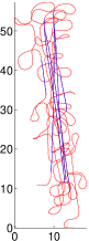
(a) Path-1

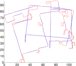
(b) Path-2

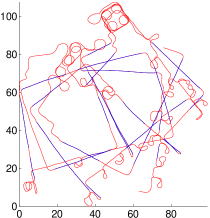
(c) Path-3

Figure 9: Straight line detection. The red lines indicate the PDR result; blue lines indicate straight-line segments identified by the straight line filter.

We show the straight line detection results in Figure 9. It shows that Path-2 and Path-3 have more straight lines detected (30 and 36 respectively) than Path-1 (only seven). This is expected because Path-2 and Path-3 went through long straight corridor areas for much more times than Path-1 did. Note that the straight line filter is not applicable for walking in office rooms and large open spaces. However, it is simply one (relatively minor) constraint used in our system to boost accuracy (Figure 12), and is more useful in reducing the ambiguity in the particle cloud (by distributing fair weights to the particles).

5.2 Loop Closure Detection and Validation

	Path-1	Path-2	Path-3
Unvalidated loop closures
Validated loop closures

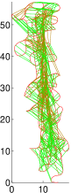
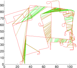
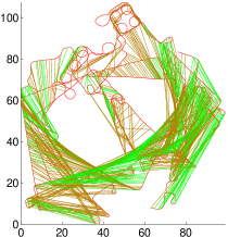
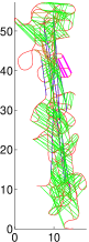
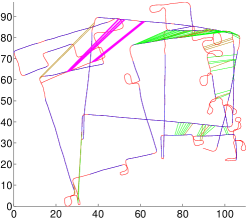
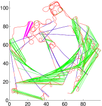
Figure 10: Loop closure validation. The green and brown lines indicate true-positive and false positive loop closures respectively.

Figure 10 illustrates the loop closures detected from the PF1-traj, drawn onto the PDR-traj (since this represents the input to PF2). In these figures green lines indicate true-positive loop closures; brown lines indicate false positive loop closures. Note that the classification of a loop closure was done post-hoc using the final trajectory—it would not be known at this stage in a live system. The bottom row shows the loop closures after validation. Very few false positives remain. The magenta-highlighted lines are true-positive closures that match to the magenta highlighted regions in Figure 11.

	Path-1		Path-2		Path-3
	Before	After	Before	After	Before	After
True	304	284	84	68	280	196
False	217	37	158	21	565	53
Ratio	0.58	0.88	0.35	0.76	0.33	0.79

TABLE I: Statistics on loop closures before and after validation.

Table I summarises the statistics on loop closures for the three paths. We observe that the validation algorithm was highly conservative as intended: it rejected a large number of closures. In all cases it significantly boosted the percentage of true loop closures above 0.7 as intended. False positives were thus moved to a minority and could not adversely impact the results (which are shown in the next Section 5.3).

5.3 Trajectory Outputs, Particle Clouds and Room Ambiguities

	Path-1	Path-2	Path-3
Trajectory
Particle cloud

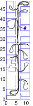
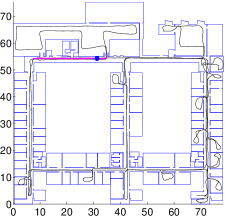
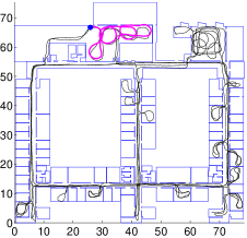
(a)

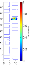
(b)

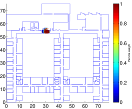
Figure 11: The results of PFSurvey on the path Path-1, Path-2 and Path-3. The magenta parts of the resultant trajectories correspond to the magenta loop closures in Figure 10.

Figure 11 shows some sample outputs from PFSurvey for the three paths. The top row shows the estimated trajectory in black, with a magenta highlight corresponding to the magenta loop closures in Figure 10. The bottom row shows the probability distribution corresponding to the positions marked with a blue dot in the top row. Note these positions match those used to generate Figure 2(f), 2(h), 4(c) and 4(f), which gave multi-modal distributions spanning multiple rooms.

We first consider Path-1. Figure 11(b) illustrates that our system has resulted in a uni-modal distribution where it was previously multi-modal, removing the room ambiguity. Figure 12 shows the CDF of the errors (made possible from the availability of high-accuracy ground truth for Path-1 [1]). Results are also shown for a typical run of the conventional filter plus smoother and the system with different components disabled. We observe that the PFSurvey result is more accurate in general: 1.1 m rather than 1.4 m 90% of the time. Note that the CDF is in some sense misleading since it does not capture the room ambiguity clearly: an error of 1 m is much more significant if it results in an erroneous room assignment than if it does not.

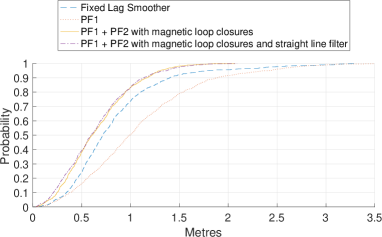
Figure 12: The error CDFs when applying a FL smoother and our proposed system on Path-1 data.

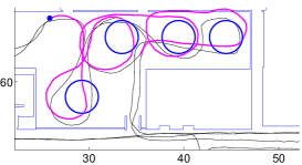
Figure 13: The estimated trajectory of Path-3 in the table area. Four large round tables (not in the floorplan) have been added.

The outputs of PFSurvey for the larger scale Path-2 and Path-3 are also shown in Figure 11. Although these survey walks did not have accurate ground truth available, the estimated paths are visually indistinguishable from the paths taken. More specifically, Path-2 and Path-3 passed 15 and 16 rooms/spaces in total respectively. The results of conventional method (Figure 4) enters five ($33.3\%$) and seven ($43.8\%$) erroneous rooms/spaces respectively; while PFSurvey result (Figure 11) achieves $100\%$ room accuracy.

The magenta-highlighted loops in Figure 11(a) result from walking around some large tables that were not in the floorplan. We subsequently measured the positions of the tables and we show them overlaid with the estimated trajectory in Figure 13 to illustrate the quality of the result from PFSurvey. Please note that a digital floor plan usually does not contain the obstacle information like furniture in the indoor environments. A particle filter using this floor plan then has only the wall information to constrain the walking path. In this case, the recovered trajectory may not be well constrained and it may go through furniture. Because many furniture can affect radio propagation, this could cause erroneous signal maps being generated. So here we have demonstrated that by incorporating the loop closure constraints in the filtering process, our system achieves high trajectory recovery accuracy even without the knowledge of furniture information. Because accurate measurement of all the furniture in indoor environments is not an easy task, and furniture sometimes can be added, moved or removed, our system is a more practical and low-cost solution for accurate path signal survey.

5.4 Signal Map and Positioning Results

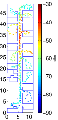
(a) PFSurvey output

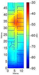
(b) GP map ($\mu$)

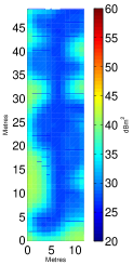
(c) GP var ($\sigma^{2}$)

Figure 14: Sample signal map.

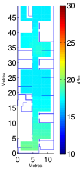
(a) RSS₉₀ map

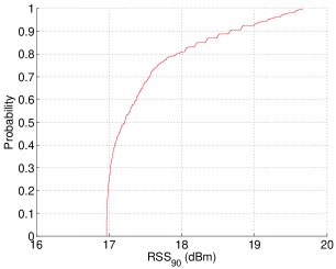
(b) CDF

Figure 15: RSS₉₀ map and CDF

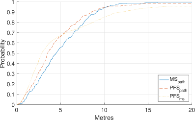
(a) Error CDF

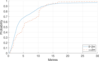
(b) Positioning CDF for PFS_ms broken down by distance from survey path

Figure 16: Positioning Results.

The primary focus of this work is the accurate estimation of a user trajectory from which to generate signal maps using path survey techniques. For completeness we also consider the subsequent stages of signal map generation and positioning. We summarise our methodology here: full details are available in [14, 13]. We used Gaussian Processes (GP) regression to generate signal maps from survey points as per [10]. Figure 14 shows the Path-1 trajectory result. Each point along the trajectory is coloured to indicate the measured signal strength of an arbitrarily chosen WiFi access point. The corresponding GP map is illustrated in Figures 14(b) and 14(c)). We assess its quality by comparison with the GP map generated from a manual survey of the same area (the manual survey is shown in Figure 1(a)). However, each position on a GP map is associated with a normal distribution rather than a scalar value so it is not trivial to compare two GP maps directly. We adopt the RSS₉₀ metric: given two Gaussian distributions, RSS₉₀ measures how much they would agree to each other. Please refer to [14] for detailed explanation.

Given two GP maps (the path survey-derived GP map and the manual survey-derived GP map), we evaluate RSS₉₀ at each grid point position in the area covered by both surveys. We visualise these RSS₉₀s by heatmap and CDF in Figure 15. They show that the agreement between the path survey map and the manual survey is good.

To evaluate the positioning performance we generated signal maps from our Path-1 dataset and used those to perform one-shot positioning based on two distinct test inputs. The first was an explicit test walk where ground truth was available through an external hi-accuracy positioning system [1]. The second was the manually-surveyed data points. Figure 16(a) shows the CDF of the positioning errors  for three distinct situations: using the PFSurvey maps to position with the test walk (PFS_path); using the PFSurvey maps to position at the manual survey points (PFS_MS); and using the manual-survey maps to position with the test walk (MS_path).

We observe that the best positioning results were achieved using the path survey when tested using the explicit test path. This is a direct consequence of that test path not straying far from the path survey input. Figure 16(b) emphasises this point: it shows the positioning errors for the PFS_MS broken down by distance of the test point from the survey path. We see that points close to the path (within 2 m) gave better accuracy. From this, it might be argued that the PFS_path line in Figure 16(a) is misleading since points far from the survey path are implicitly excluded. However, we would expect a dedicated surveyor to walk through all accessible areas following the most likely paths (e.g. centre line of the corridor). As such the most common positioning requests will be close to the path survey trajectory and the PFS_path line is then a more realistic evaluation.

We further note that the maps generated by PFSurvey and those generated from the manual survey achieve a similar accuracy, despite the cost of gathering the data being significantly lower for PFSurvey. In our experience PFSurvey replaces a laborious manual survey that takes many hours with a simple walk lasting a few minutes.

6 Conclusions

In this paper we have described and evaluated PFSurvey, a system designed to allow a dedicated surveyor to build a signal survey for a space in a matter of minutes using a commodity smartphone, assuming a floorplan of the space is available. The system uses a series of pre-processing steps to generate reliable loop closures between points on a noisy dead-reckoned trajectory. These are then fused with the floorplan to provide a robust, accurate trajectory that can be used to generate maps of any quantity measured during the survey.

We have evaluated PFSurvey in a large building and shown that it can successfully solve the room ambiguity problem that typically results from using solely the floorplan to constrain the dead-reckoning drift. We have demonstrated that the PFSurvey trajectory can be used to build detailed signal maps that allow positioning accuracy on a par with conventional, laborious manual surveying.

Chao Gao received the BS degree in 2011 from Harbin Institute of Technology, China and the M.Phil. and Ph.D. degrees in 2013 and 2017 from the University of Cambridge, UK. His research interests include indoor positioning, mapping and robotics.

Robert Harle received the Ph.D. degree from the University of Cambridge, UK, in 2005. He is currently a Senior Lecturer at the Cambridge University Computer Laboratory. His current research interests include mobile, wireless and ubiquitous computing, including mobile health, positioning and the Internet of Things.

References

- [1] M. Addlesee, R. Curwen, S. Hodges, J. Newman, P. Steggles, A. Ward, and A. Hopper. Implementing A Sentient Computing System. IEEE Computer, 34(8), August 2001.
- [2] K. Al Nuaimi and H. Kamel. A survey of indoor positioning systems and algorithms. In Innovations in Information Technology (IIT), 2011 International Conference on, pages 185–190. IEEE, 2011.
- [3] P. Bahl and V. Padmanabhan. RADAR: An in-building RF-based user location and tracking system. In INFOCOM 2000. Nineteenth Annual Joint Conference of the IEEE Computer and Communications Societies. Proceedings. IEEE, volume 2, pages 775–784. IEEE, 2000.
- [4] A. Brajdic and R. Harle. Walk detection and step counting on unconstrained smartphones. In Proceedings of the 2013 ACM international joint conference on Pervasive and ubiquitous computing, pages 225–234. ACM, 2013.
- [5] X. Chai and Q. Yang. Reducing the calibration effort for probabilistic indoor location estimation. IEEE Transactions on Mobile Computing, 6(6):649–662, 2007.
- [6] K. Chintalapudi, A. Padmanabha Iyer, and V. N. Padmanabhan. Indoor localization without the pain. In Proceedings of the sixteenth annual international conference on Mobile computing and networking, pages 173–184. ACM, 2010.
- [7] A. Doucet, S. Godsill, and C. Andrieu. On sequential Monte Carlo sampling methods for Bayesian filtering. Statistics and computing, 10(3):197–208, 2000.
- [8] A. Eliazar and R. Parr. DP-SLAM: Fast, Robust Simultaneous Localization and Mapping without Predetermined Landmarks. In in Proc. 18th Int. Joint Conf. on Artificial Intelligence (IJCAI-03, pages 1135–1142. Morgan Kaufmann, 2003.
- [9] B. Ferris, D. Fox, and N. Lawrence. WiFi-SLAM using Gaussian process latent variable models. In Proceedings of the 20th international joint conference on Artifical intelligence, IJCAI’07, pages 2480–2485, San Francisco, CA, USA, 2007. Morgan Kaufmann Publishers Inc.
- [10] B. Ferris, D. Haehnel, and D. Fox. Gaussian processes for signal strength-based location estimation. In In proc. of robotics science and systems. Citeseer, 2006.
- [11] D. Fox. KLD-sampling: Adaptive particle filters. In Advances in neural information processing systems, pages 713–720, 2001.
- [12] D. Fox. Adapting the sample size in particle filters through KLD-sampling. The international Journal of robotics research, 22(12):985–1003, 2003.
- [13] C. Gao and R. Harle. Sequence-based magnetic loop closures for automated signal surveying. In Indoor Positioning and Indoor Navigation (IPIN), 2015 International Conference on, pages 1–12. IEEE, 2015.
- [14] C. Gao and R. Harle. Easing the Survey Burden: Quantitative Assessment of Low-Cost Signal Surveys for Indoor Positioning. In Indoor Positioning and Indoor Navigation (IPIN), 2016 International Conference on, pages 1–8. IEEE, 2016.
- [15] T. Giorgino. Computing and visualizing dynamic time warping alignments in R: the dtw package. Journal of statistical Software, 31(7):1–24, 2009.
- [16] S. J. Godsill, S. J. Godsill, A. Doucet, and M. West. Monte Carlo smoothing for non-linear time series. JOURNAL OF THE AMERICAN STATISTICAL ASSOCIATION, 99:156–168, 2004.
- [17] Y. Gu, A. Lo, and I. Niemegeers. A survey of indoor positioning systems for wireless personal networks. Communications Surveys Tutorials, IEEE, 11(1):13–32, quarter 2009.
- [18] D. Han, S. Jung, M. Lee, and G. Yoon. Building a practical Wi-Fi-based indoor navigation system. IEEE Pervasive Computing, 13(2):72–79, 2014.
- [19] V. Honkavirta, T. Perala, S. Ali-Loytty, and R. Piche. A comparative survey of WLAN location fingerprinting methods. In Positioning, Navigation and Communication, 2009. WPNC 2009. 6th Workshop on, pages 243–251, March 2009.
- [20] A. K. M. M. Hossain, Y. Jin, W.-S. Soh, and H. N. Van. SSD: A Robust RF Location Fingerprint Addressing Mobile Devices’ Heterogeneity. IEEE Trans. Mob. Comput., 12(1):65–77, 2013.
- [21] J. Huang, D. Millman, M. Quigley, D. Stavens, S. Thrun, and A. Aggarwal. Efficient, generalized indoor WiFi GraphSLAM. In Robotics and Automation (ICRA), 2011 IEEE International Conference on, pages 1038–1043, May.
- [22] S.-h. Jung, B.-c. Moon, and D. Han. Unsupervised learning for crowdsourced indoor localization in wireless networks. IEEE Transactions on Mobile Computing, 15(11):2892–2906, 2016.
- [23] M. B. Kjærgaard. Indoor location fingerprinting with heterogeneous clients. Pervasive and Mobile Computing, 7(1):31–43, 2011.
- [24] M. Klepal and S. Beauregard. A Backtracking Particle Filter for fusing building plans with PDR displacement estimates. 2008 5th Workshop on Positioning Navigation and Communication, 2008:207–212, 2008.
- [25] H. Koyuncu and S. H. Yang. A survey of indoor positioning and object locating systems. IJCSNS International Journal of Computer Science and Network Security, 10(5):121–128, 2010.
- [26] B. Krach and P. Robertson. Integration of foot-mounted inertial sensors into a Bayesian location estimation framework. 2008 5th Workshop on Positioning Navigation and Communication, 2008(2):55–61, 2008.
- [27] B. Li, T. Gallagher, A. G. Dempster, and C. Rizos. How feasible is the use of magnetic field alone for indoor positioning? In Indoor Positioning and Indoor Navigation (IPIN), 2012 International Conference on, pages 1–9. IEEE, 2012.
- [28] H. Liu, H. Darabi, P. Banerjee, and J. Liu. Survey of wireless indoor positioning techniques and systems. Systems, Man, and Cybernetics, Part C: Applications and Reviews, IEEE Transactions on, 37(6):1067–1080, 2007.
- [29] M. Montemerlo, S. Thrun, D. Koller, B. Wegbreit, et al. FastSLAM: A factored solution to the simultaneous localization and mapping problem. In AAAI/IAAI, pages 593–598, 2002.
- [30] J. J. Pan, S. J. Pan, J. Yin, L. M. Ni, and Q. Yang. Tracking mobile users in wireless networks via semi-supervised colocalization. IEEE transactions on pattern analysis and machine intelligence, 34(3):587–600, 2012.
- [31] A. Rai, K. K. Chintalapudi, V. N. Padmanabhan, and R. Sen. Zee: zero-effort crowdsourcing for indoor localization. In Proceedings of the 18th annual international conference on Mobile computing and networking, pages 293–304. ACM, 2012.
- [32] H. Wang, S. Sen, A. Elgohary, M. Farid, M. Youssef, and R. R. Choudhury. No need to war-drive: unsupervised indoor localization. In Proceedings of the 10th international conference on Mobile systems, applications, and services, pages 197–210. ACM, 2012.
- [33] O. Woodman and R. Harle. Pedestrian localisation for indoor environments. In Proceedings of the 10th international conference on Ubiquitous computing, pages 114–123. ACM, 2008.
- [34] O. J. Woodman. Pedestrian localisation for indoor environments. Phd thesis, Computer Laboratory, University of Cambridge, September 2010.
- [35] C. Wu, Z. Yang, and Y. Liu. Smartphones based crowdsourcing for indoor localization. IEEE Transactions on Mobile Computing, 14(2):444–457, 2015.
- [36] C. Wu, Z. Yang, Y. Liu, and W. Xi. WILL: Wireless indoor localization without site survey. IEEE Transactions on Parallel and Distributed Systems, 24(4):839–848, 2013.
- [37] M. Youssef and A. Agrawala. The Horus WLAN location determination system. In Proceedings of the 3rd international conference on Mobile systems, applications, and services, MobiSys ’05, pages 205–218, New York, NY, USA, 2005. ACM.