Pseudocanalization regime for magnetic dark-field hyperlenses

Abstract

Hyperbolic metamaterials (HMMs) are the cornerstone of the hyperlens, which brings the superresolution effect from the near-field to the far-field zone. For effective application of the hyperlens it should operate in so-called canalization regime, when the phase advancement of the propagating fields is maximally supressed, and thus field broadening is minimized. For conventional hyperlenses it is relatively straightforward to achieve canalization by tuning the anisotropic permittivity tensor. However, for a dark-field hyperlens designed to image weak scatterers by filtering out background radiation (dark-field regime) this approach is not viable, because design requirements for such filtering and elimination of phase advancement i.e. canalization, are mutually exclusive. Here we propose the use of magnetic ($\mu$-positive and negative) HMMs to achieve phase cancellation at the output equivalent to the performance of a HMM in the canalized regime. The proposed structure offers additional flexibility over simple HMMs in tuning light propagation. We show that in this “pseudocanalizing” configuration quality of an image is comparable to a conventional hyperlens, while the desired filtering of the incident illumination associated with the dark-field hyperlens is preserved.

I Introduction

The diffraction limit has been a notorious challenge in a wide range of applications. Optical subwavelength imaging is one particularly active research direction and throughout the years various solutions have been proposed to circumvent the diffraction limit. So far practical results have emerged from a variety of scanning techniques: scanning near-field optical microscopy (SNOM) Dunn (1999) and more recently stimulated emission depletion (STED) microscopy Hell and Wichmann (1994); Klar and Hell (1999). Given the intrinsic slowness of scanning methods, there has always been an interest in alternative ways to achieve superresolution imaging. With advances in nanofabrication methods optical metamaterials have become a very promising research direction. The idea of using metamaterials for superresolution is also not particularly new — Pendry Pendry (2000) has proposed to use a double-negative metamaterial to form a superlens, which would be able to image details below the diffraction limit. The superlens itself is somewhat limited in its applicability, as practical considerations restrict experimental realizations of such device Jacob et al. (2006). A few years later an alternative approach which avoided double-negative media was proposed Jacob et al. (2006) and experimentally demonstrated Liu et al. (2007). This design (the hyperlens) was instead based on a hyperbolic metamaterial (HMM) structure for superresolution. The HMM based design allows to avoid the practical challenges of superlenses: unlike double-negative metamaterials fabrication of the HMMs is not so challenging, as they do not rely on resonant parts. More importantly, due to their non-resonant nature the HMM structures are less affected by inevitable material losses especially in the visible Jacob et al. (2006); Yao et al. (2008); Valentine et al. (2008).

A hyperbolic medium is an anisotropic medium, where the ordinary and extraordinary permitivitties have opposing signs. Effectively, the medium is metallic in one direction and dielectric in others. In solving this system for plane wave propagation the resulting dispersion relation shows that waves with arbitrarily high wavevectors are allowed to propagate inside the medium [i.e. the isofrequency surface $\omega=f\left(k_{x},k_{y},k_{z}\right)=\mathrm{const}$ is unbounded] Smith and Schurig (2003); Liu et al. (2008); Poddubny et al. (2013). This is in contrast to conventional media, where only a limited range of waves can propagate, while the rest are evanescent. The evanescent waves are highly localized and are only accessible by near-field probes (such as SNOM) Novotny and Hecht (2006). This filtering of high-k waves in the far field results in the diffraction limit. The ability of hyperbolic media to carry these waves allows for superresolution imaging by subverting the diffraction limit.

To facilitate a straightforward imaging process, the hyperlens should be designed such that the fields propagate through the device with minimal distortion Lu and Liu (2012); Xiong et al. (2009); Ikonen et al. (2007); Rho et al. (2010). This is achieved when the HMM is engineered to have the permittivity tensor [$\hat{\varepsilon}=\mathrm{diag}(\varepsilon_{x},\varepsilon_{y},\varepsilon_{x})$] feature either the epsilon-near-zero ($\varepsilon_{x}\approx 0$) or epsilon-near-pole ($|\varepsilon_{y}|\gg 1$) components (i.e. the HMM is operated in the so-called canalization regime). As a consequence the plane wave field components acquire very little phase, meaning that the image is effectively “canalized” through the medium, exhibiting very little broadening or diffraction.

Natural objects for superresolution imaging would be biological samples in scale of a few hundred nanometers, which are relatively weakly scattering (compared to plasmonic particles, for example). As the usual design of the hyperlens carries both incident and scattered waves the available contrast is not enough in case of weakly scattering objects. To facilitate imaging of weakly scattering subwavelength objects, dark-field hyperlens designs were proposed Benisty and Goudail (2012); Repän et al. (2015). For example, by appropriately choosing signs of the permittivity tensor components Repän et al. (2015) a hyperbolic medium can be engineered to filter out waves with long effective wavelength (small wavenumber). This mode of operation (termed type-II HMM) can be used as a basis for a dark field hyperlens Repän et al. (2015). However, the design based on type-II HMM suffers from the lack of canalization regime and reduced device performance.

In this paper, we propose a new method for circumventing the diffraction limit using a canalization regime. In doing this, we provide a detailed discussion of wave propagation in hyperbolic materials with special emphasis to canalization solutions. We show from the propagation equations that the image broadening in hyperbolic media has two different contributions: absorption (determined by material losses) and phase accumulation (determined by the dispersion relation). The absorption term is difficult to circumvent, but the phase propagation may be decreased (for example by employing the canalization regime). However, we show that the canalization regime for a homogeneous hyperbolic medium is fundamentally incompatible with dark-field imaging (based on low-k filtering). Relaxing the requirement of a homogeneous medium leads to the idea of a “pseudocanalization” regime, where instead of a single medium we aim to use two complementary media to compensate phase advances of each other (allowing for reduced broadening), while keeping the low-k filtering properties necessary for dark-field imaging. This complementary medium can be realized using a $\mu$-negative HMM, extending the idea for isotropic media from Ref. Alu and Engheta, 2003.

We start by outlining basic theory of light propagation in HMMs in Section II. We follow with discussion about the canalization regime in hyperbolic media (Section III). In Section IV we propose and discuss the idea of pseudocanalization by using $\mu$-negative HMMs for phase compensation. We demonstrate applicability of the idea in Section V, with particular focus on improving a dark-field hyperlens.

II Basic theory

II.1 Propagation of waves and dispersion equation

To study propagation of plane waves in homogeneous medium we consider an angular spectrum representation Novotny and Hecht (2006) of the fields, where the initial electric fields at $y=0$ are decomposed with the Fourier transform

$$\mathbf{E}\left(k_{x},y=0\right)=\frac{1}{2\pi}\intop\mathbf{E}\left(x,y=0\right)\exp\left(-ik_{x}x\right)dx\,.$$ (1)

Propagated fields after a distance $y$ can then be calculated with

$$\mathbf{E}\left(k_{x},y\right)=\mathbf{E}\left(k_{x},y=0\right)\exp\left(ik_{y}y\right)\,,$$ (2)

where $k_{y}$ is the propagation constant (wavevector component along the $y$-axis). Using an inverse Fourier transformation, we find:

$$\mathbf{E}\left(x,y\right)=\intop\mathbf{E}\left(k_{x},y\right)\exp\left(ik_{x}x\right)dk_{x}\,.$$ (3)

To apply Eq. (2) for HMMs we need the expression for the propagation constant $k_{y}$ in an anisotropic medium. We assume an anisotropic permittivity [$\hat{\varepsilon}=\mathrm{diag}\left(\varepsilon_{x},\varepsilon_{y},\varepsilon_{x}\right)$] and an isotropic permeability ($\mu$). Assuming next a plane wave solution for Maxwell’s equations the dispersion relation for extraordinary waves becomes (see details in Appendix A)

$$\frac{k_{x}^{2}+k_{z}^{2}}{\varepsilon_{y}}+\frac{k_{y}^{2}}{\varepsilon_{x}}=\mu k_{0}^{2}\,,$$ (4)

which describes propagation of plane waves through the medium. In this paper we assume propagation in the $x$-$y$ plane, i.e. $k_{z}=0$. We can solve Eq. (4) to yield the propagation constant in the $y$-direction

$$k_{y}=\pm\sqrt{\varepsilon_{y}\varepsilon_{x}\left(\varepsilon_{y}k_{0}^{2}\mu-k_{x}^{2}\right)}/\varepsilon_{y}\,.$$ (5)

The sign of $k_{y}$ can be established using the Poynting vector direction – we are interested in waves propagating towards the positive $y$ direction. The $y$-component of the Poynting vector in our case can be written as

$$S_{y}=\frac{\left|H_{z}\right|^{2}}{2\omega}\mathrm{Re}\left(\frac{k_{y}}{\varepsilon_{0}\varepsilon_{x}}\right)\,.$$ (6)

To have propagation in the positive $y$ direction, the sign of $k_{y}$ must be chosen to have $S_{y}>0$.

In the general case the propagation constant has both real and imaginary parts $k_{y}=k_{y}^{\prime}+\mathrm{i}k_{y}^{\prime\prime}$, where the real (imaginary) part describes phase accumulation (attenuation).

II.2 Propagation in hyperbolic media

In hyperbolic media components $\varepsilon_{x}$, $\varepsilon_{y}$ have different signs. In this case the isofrequency contour of Eq. (4) will yield a hyperboloid, as shown in Fig. 1(a,b). Two different configurations can be distinguished: we designate the case of $\mu\varepsilon_{y}<0<\mu\varepsilon_{x}$ as type-I hyperbolic dispersion and the case of $\mu\varepsilon_{x}<0<\mu\varepsilon_{y}$ an type-II hyperbolic dispersion Shekhar et al. (2014). We note that asymptotic behavior for large $k_{x}$ is the same for type-I and type-II hyperbolic media:

$$k_{y}\propto\pm k_{x}\sqrt{\left|\varepsilon_{x}\right|/\left|\varepsilon_{y}\right|}\,.$$ (7)

This indicates that $k_{y}$ will stay real for arbitrary high $k_{x}$ and consequently the high-k waves are always propagating waves in the hyperbolic medium. This is different from conventional media, where the propagation constant for high-k waves turns fully imaginary, signifying evanescent nature of the fields Novotny and Hecht (2006).

The differences between type-I and type-II hyperbolic media become apparent for low-k waves. The propagation constant at $k_{x}=0$ becomes

$$k_{y}\left(0\right)=\pm\sqrt{\varepsilon_{x}k_{0}^{2}\mu}\,.$$ (8)

For type-II HMM $\varepsilon_{x}\mu<0$ so the propagation constant becomes imaginary, i.e. these waves are evanescent (for conventional medium) or amplified (in case of gain medium). The transition point $k_{c}$ between low-k and high-k waves can be seen from Eq. (5) :

$$k_{c}^{2}=\varepsilon_{y}\mu k_{0}^{2}\,,$$ (9)

meaning that in a type-II HMM only waves with $\left|k_{x}\right|\geq k_{c}$ (high-k) will be propagating, whereas waves with $\left|k_{x}\right|<k_{c}$ (low-k) will be evanescent. As the subwavelength details of an image are mostly contained in high-k waves,while the background field is transported by low-k waves, this filtering can be used to design a dark-field version of the hyperlens Repän et al. (2015). We use Eq. (2) to calculate the propagation of the fields through the hyperbolic medium to illustrate the key difference between type-I and type-II HMMs, namely the filtering of background radiation in type-II hyperbolic medium. Figure 1(c,d) shows that the type-II HMM filters out background radiation, unlike the type-I HMM.

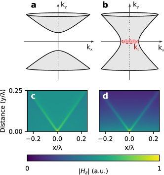
Figure 1: (a,b) Isofrequency surfaces for type-I (a) and type-II (b) hyperbolic dispersions. The surfaces are unbounded, allowing propagation of waves with arbitrarily large $k_{x}$. However, in type-II HMM (b) the low-k waves ($k_{x}<k_{c}$) are not propagating waves (marked with red circle). (c,d) Propagation of fields from a point source along with uniform background fields in type-I HMM $\varepsilon_{x}=1+0.05\mathrm{i}$, $\varepsilon_{y}=-1+0.05\mathrm{i}$ (c) and type-II HMM $\varepsilon_{x}=-1+0.05\mathrm{i}$, $\varepsilon_{y}=1+0.05\mathrm{i}$ (d). Important feature of type-II HMM is that the background fields are attenuated along propagation.

III Canalization regime

One of the early proposals for a hyperlens was based on a metamaterial consisting of a wire medium Belov et al. (2006). In such a medium the modes propagating in individual wires transport pixels of the image. In other words, the image is “canalized” from the inner to outer interface, giving rise to the name of this mode of operation. This is important for imaging purposes, as the fields propagate with minimal distortion. However, such operation is not limited to wire media: similar operation can be obtained with various configurations of hyperbolic metamaterials Salandrino and Engheta (2006); Jacob et al. (2007); Lee et al. (2007). In general, a hyperbolic medium approaches the canalization regime as either $\varepsilon_{x}$ approaches zero and/or $\varepsilon_{y}$ approaches infinity. In these limits the propagation constant becomes independent of $k_{x}$ and from Eq. (3) it follows that fields will propagate in an undistorted manner:

$$\mathbf{E}(x,y)=\exp\left(ik_{y}y\right)\mathbf{E}\left(x,0\right)\,.$$ (10)

As a result, fields are “canalized” through the medium. For superresolution imaging this regime is strongly desirable, as it is vital for a distortion-free image. Most hyperlens designs proposed so far utilize the canalization regime. For a detailed discussion on HMMs where $\varepsilon_{x}\approx 0$ see Ref. Castaldi et al., 2012.

The canalization regime also implies minimal broadening of the image. For waves propagating in $y$-direction, we can estimate broadening using the Poynting vector components:

$$\frac{S_{x}}{S_{y}}=\frac{\mathrm{Re}\left(k_{x}/\varepsilon_{y}\right)}{\mathrm{Re}\left(k_{y}/\varepsilon_{x}\right)}\,,$$ (11)

which in canalization limit approaches zero (for the lossless case). This shows that in a canalizing system the fields propagate directly in $y$-direction, i.e. there is no broadening. In lossy systems the broadening will have two contributions: one arises from attenuation of waves which affects high-k waves more and thus narrows the spectrum in the reciprocal space. This corresponds to broadening in the real space. Furthermore, spread of the Poynting vector [as per Eq. (11)] also causes broadening. This spread is linked to the phase accumulation of propagating fields and can therefore, in principle, be compensated. For comparison, compensating for attenuation losses is impossible without using gain media.

It is important to note that the distinction between a type-I and type-II HMM disappears in the canalization regime. Firstly, considering the limit where $\varepsilon_{y}\to\infty$, we see from Eq. (5) that $k_{y}\approx\sqrt{\varepsilon_{x}\mu}k_{0}$ (for large $\varepsilon_{y}$), which means that all fields will be either propagating or evanescent, depending on the sign of $\varepsilon_{x}\mu$. As a consequence, there is no distinction between low-k and high-k waves. In other case ($\varepsilon_{x}\to 0$) we see that the distinction between low-k and high-k waves is unaltered [the cut-off point $k_{c}$ is independent of $\varepsilon_{x}$, as per Eq. (9)]. However, from Eq. (5) it follows that the propagation constant $k_{y}$ scales with $\sqrt{\varepsilon_{x}}$. This means that as the system moves closer to the canalization regime the attenuation constant ($\mathrm{Im}\,k_{y}$) is reduced therefore nullifying the low-k filtering effect.

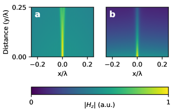
Figure 2: Propagation of fields through a canalizing (a) and a pseudocanalizing (b) type-II HMM slab. The canalizing HMM parameters are $\varepsilon_{x}=\left(-1+0.05\mathrm{i}\right)/20^{2}$, $\varepsilon_{y}=1+0.05\mathrm{i}$. To achieve pseudocanalization a slab of type-II HMM [same as in Fig. 1(d)] is combined with a compensating slab [given by Eqs. (17) and (18), with $\mu^{(2)}=-1$] of equal thickness. Initial field is the superposition of the field of a narrow point-like source and a uniform background field. Note that unlike the noncanalizing type-II HMM [Fig. 1(d)], there is no attenuation of the background fields in (a). However, in the pseudocanalizing system (b) the background filtering properties are restored.

The lack of low-k filtering is shown in Fig. 2(a), which shows that in the canalization regime the type-II HMM does not attenuate background fields [compare against Fig. 1(d)]. As the background fields are not attenuated, the canalization regime is not applicable for dark-field imaging. However, working beyond the canalization regime degrades the image quality of hyperlens, creating additional challenges Repän et al. (2015). Therefore, it would be beneficial to achieve canalization-like behavior while still maintaining the low-k filtering properties.

From the propagation equation [Eq. (2)] we note that the effect of the propagation constant $k_{y}$ can be split into the real ($k_{y}^{\prime}$) and imaginary ($k_{y}^{\prime\prime}$) parts. The real part will yield a phase term [$\exp\left(ik_{y}^{\prime}y\right)$], while the other term yields an attenuating term [$\exp\left(-k_{y}^{\prime\prime}y\right)$]. The latter affects the high-k waves more, causing narrowing of the wavevector spectrum (broadening in the image space). This broadening is shown in Fig. 3(a), where only the attenuation term is taken into account. However, the phase term will also contribute to broadening, as seen in Fig. 3(b), where both phase and attenuation terms are considered. Comparing the two cases [Fig. 3(c)], we see that phase term causes additional broadening. As the canalization regime implies minimal phase distortions, the additional broadening term is suppressed in this regime.

Figure 3: Broadening of the fields during propagation through type-II HMM ($\varepsilon_{x}=-1+\mathrm{i}\gamma$, $\varepsilon_{y}=1+\mathrm{i}\gamma$, $\gamma=0.1$). Propagation of fields through the slab, for normal type-II slab (b) and for phase-less propagation, i.e. $\mathrm{Re}\,k_{y}=0$ (a). FWHM of the beam with various losses is indicated by the solid ($\gamma=0.1$), dashed ($\gamma=0.2$) and dotted ($\gamma=0.05$) lines. (c) Fields for both cases (normal and phase-less propagation) after propagation distance $z=0.2$. The dashed and dotted lines indicate the same loss factors $\gamma$. The results indicates that the phase term is responsible for having $\sim 2\times$ increase in FWHM.

IV Phase compensation with $\mu$-negative HMM

The key property of the canalization regime (in the ideal limit) is that fields propagate with constant phase accumulation [i.e. $\mathrm{Re}\left(k_{y}\right)=\mathrm{const}$]. However, the canalization regime is not a strict prerequisite for having no phase accumulation. The identical result could be achieved by replacing the homogeneous HMM medium with two different HMM slabs with complementary dispersion, such that

$$d_{1}k_{y}^{(1)}\left(k_{x}\right)=-d_{2}k_{y}^{(2)}\left(k_{x}\right)\,,$$ (12)

where $d_{1}$, $d_{2}$ are the thicknesses of two slabs. In most of the calculations here we assumed $d_{1}=d_{2}$, but in general thicknesses can be varied to allow more freedom in engineering suitable permittivity and permeability properties. Assuming full impedance matching (ie. no reflections) between the slabs, the propagated fields will have no distortions in the phase or amplitude. In this case the two slabs form effectively a canalizing system.

To proceed with calculations, we assume two lossless hyperbolic media: the first medium has $\mu^{(1)}=1$, whereas for the second medium we require $\mu^{(2)}<0$. We can repeat Eq. (12) for the two defining cases, firstly for low-k waves ($k_{x}=0$)

$$d_{1}\mathrm{sgn}\left(\varepsilon_{y}^{(1)}\right)\sqrt{\varepsilon_{x}^{(1)}}=-d_{2}\mathrm{sgn}\left(\varepsilon_{y}^{(2)}\right)\sqrt{\mu^{(2)}\varepsilon_{x}^{(2)}}\,,$$ (13)

and then for high-k waves by taking the limit where $k_{x}$ approaches infinity:

$$d_{1}\sqrt{-\varepsilon_{x}^{(1)}\varepsilon_{y}^{(1)}}k_{x}/\varepsilon_{y}^{(1)}=-d_{2}\sqrt{-\varepsilon_{x}^{(2)}\varepsilon_{y}^{(2)}}k_{x}/\varepsilon_{y}^{(2)}\,.$$ (14)

Solving Eqs. (13) and (14) yields conditions for two slabs:

$$\mu^{(2)}\varepsilon_{x}^{(2)} = \varepsilon_{x}^{(1)}d_{1}^{2}/d_{2}^{2}$$ (15)

$$\mu^{(2)}\varepsilon_{y}^{(2)} = \varepsilon_{y}^{(1)}\,.$$ (16)

Although we derived the relations based only on two cases ($k_{x}=0$ and $k_{x}=\infty$), it is easy to verify that the phase-matching condition [Eq. (12)] holds for all $k_{x}$. In case of lossy media, we limit the discussion to media where $\mathrm{Im}\left(\varepsilon\right)>0$, i.e. we neglect gain media. In lossy media we only require the real part of Eq. (12) to hold. However, we do assume $d_{1}\mathrm{Im}\,k_{y}^{(1)}=d_{2}\mathrm{Im}\,k_{y}^{(2)}$, so that we reach the following conditions for complex permitivitties:

$$\mu^{(2)}\varepsilon_{x}^{(2)} =\varepsilon_{x}^{(1)*}d_{1}^{2}/d_{2}^{2}$$ (17)

$$\mu^{(2)}\varepsilon_{y}^{(2)} =\varepsilon_{y}^{(1)*}$$ (18)

The conditions above ensure that the phase accumulation is canceled even in lossy media. However, due to losses the fields will not stay unmodified — the plane wave components of the image will be attenuated, where attenuation factor $\mathrm{Im}\left(k_{y}\right)$ depends on $k_{x}$. As different plane wave components experience different attenuation, this will result in broadening of the image in real space. However, as discussed in the previous section, the broadening in HMMs is caused both by phase and attenuation terms. In a pseudocanalizing system the contribution from the phase term is eliminated. Figure 3(c) shows that even when considering the losses, the broadening is greatly reduced in a pseudocanalizing system.

It is important to stress that the constituent media are not required to be in the canalization regime. This means that we can have two complementary type-II HMM slabs (both exhibiting low-k filtering) and combine them in the pseudocanalizing system with dark-field operation.

From the impedance for oblique incidence ($\gamma=k_{y}/\varepsilon_{x}k_{0}$), conditions for slab permitivitties [Eqs. (15) and (16)] and wavenumbers Eq. (12) we see that the pseudocanalizing slabs are impedance matched, for the lossless case. As the designs of practical interest are limited to low loss regime, we continue to neglect reflections for lossy system as well. We later show with full-wave simulations that reflections do not significantly alter performance of the device. Therefore propagation of the initial fields through the two slabs can be written in accordance with Eq. (2) as

$$\mathbf{E}\left(k_{x},y\right)=\begin{cases}\mathbf{E}\left(k_{x},0\right)\exp\left(ik_{y}^{(1)}y\right)&y<h\\ \mathbf{E}\left(k_{x},0\right)\exp\left(ik_{y}^{(1)}h\right)\exp\left(ik_{y}^{(2)}\left(y-h\right)\right)&y>h\end{cases}\,,$$ (19)

where $h$ is the thickness of the first slab. In Fig. 2(b) we use this to show operation of such pseudocanalizing system. We see that the original image is transmitted with minimal distortion (similar to the canalizing medium), except for the background, which is strongly attenuated.

However, as shown in Fig. 4, the image from the type-II pseudocanalizing system is not completely distortion-free: attenuation of low-k waves behaves as a high-pass filter for the image, somewhat reducing the image quality. The $\exp\left(ik_{y}y\right)$ term in the propagation equation [Eq. (3)] can be approximated as a high-pass filter with the cut-off at $k_{c}$. Assuming a point source, we can use the Fourier transform of a rectangular function to approximate the filtered image as

$$\mathbf{E}\left(x,y\right)\approx\mathbf{E}_{0}\frac{2}{x}\sin\left(k_{c}x\right)\,.$$ (20)

We see that due to filtering the image will have additional zeros at $n\pi/k_{c}$ (with $n=0,\pm 1,...$). This is made worse with increasing $k_{c}$ , as the image will develop more sidelobes.

Finally, it’s worth pointing out that the phase compensation could be achieved in limited cases without $\mu$-negative materials as well. It is easy to show that phase compensation condition for high-k waves [Eq. (14)] will have the same form even when $\mu^{(2)}=\mu^{(1)}=1$. This means that phase compensation can be achieved with a medium where

$$\mathrm{sgn}\left(\varepsilon_{y}^{(1)}\right) = -\mathrm{sgn}\left(\varepsilon_{y}^{(2)}\right)\,,$$ (21)

$$\varepsilon_{x}^{(1)}/\varepsilon_{y}^{(1)} = \left(\varepsilon_{x}^{(2)}d_{1}^{2}\right)/\left(\varepsilon_{y}^{(2)}d_{2}^{2}\right)\,.$$ (22)

This only partially solves the problem since for low-k waves the phase is not canceled [Eq. (13) is not satisfied]. For example, in superresolution imaging applications most of the energy will be carried by waves with $k_{x}$ near $k_{c}$, both due to their evanescent nature in the medium outside the hyperlens and also due to material losses having stronger effect on waves with higher $k_{x}$. Since the phase of waves near $k_{c}$ is not compensated the image will experience significant distortion.

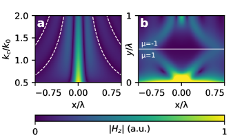
Figure 4: (a) Magnetic fields after propagation of a fixed distance ($y=\lambda$, $h=\lambda/2$) of pseudocanalizing type-II HMM, with varying low-k cutoff $k_{c}$. Dashed lines indicate expected zeros at $n\pi/k_{c}$, present due low-k filtering. Material parameters are $\varepsilon_{x}=-k_{c}^{2}/k_{0}^{2}$, $\varepsilon_{y}=k_{c}^{2}/k_{0}^{2}$. Initial fields are $H_{z}=\exp\left(-x^{2}/\Delta^{2}\right)$, where $\Delta=\lambda/10$. (b) Operation of pseudocanalizing system for $k_{c}=1.5k_{0}$. The figures are calculated using Eq. (19).

V Pseudocanalization in a cylindrical hyperlens

We now extend the discussion from planar to cylindrical geometry as is the case with hyperlens structures. For cylindrical geometry the hyperbolic permittivity is given as $\hat{\varepsilon}=\mathrm{diag}\left(\varepsilon_{\theta},\varepsilon_{r},\varepsilon_{\theta}\right)$. A simple plane wave analysis suffices for a qualitative understanding. The detailed numerics is carried out using a full-wave EM analysis. From geometric principles it follows straightforwardly that the image is expanded by a factor of

$$M=\frac{r_{2}}{r_{1}}\,,$$ (23)

where $r_{1}$ is the initial radius from which the fields start propagating (inner surface of the hyperlens) and $r_{2}$ is the final radius (outer surface of the hyperlens). In angular spectrum representation this corresponds to a compression of $k_{\theta}$ as the wave propagates from the initial value $k_{\theta}^{\prime}$ to

$$k_{\theta}=k_{\theta}^{\prime}/M\,,$$ (24)

where $k_{\theta}^{\prime}$ is the initial value. To counteract effects of magnification, the second medium (compensation medium) should be scaled. As we show in Appendix B, $\varepsilon_{r}^{(2)}$ should be scaled by the total magnification of the hyperlens:

$$\varepsilon_{r}^{(2)}=\varepsilon_{r}^{\prime(2)}/M\,.$$ (25)

To demonstrate the concept, we have chosen relatively simple material parameters for the HMMs, of the form $\varepsilon_{x,y}=\pm 1+\gamma\mathrm{i}$. This allows us to capture the effects related to losses, while keeping the number of free parameters minimal. However, we point out the choice is only done to demonstrate a simple analysis, as the conditions in Eqs. (17) and (18) are general and are not limited to the simplifed paramaters used here.

We start by demonstrating the concept with a bright field hyperlens [Fig. 5(a)], based on a type-I HMM. This allows us to directly compare canalizing and pseudocanalizing operations in cylindrical geometry. We show that the pseudocanalizing system works in cylindrical geometry too [Fig. 5(b)], demonstrating applicability for hyperlens devices. Figure 5 is obtained by full-wave simulations (using COMSOL Multiphysics v5.1), i.e. reflections from interfaces are taken into account. Standing waves originated from these reflections are seen on the figures as the modulated intensity along the direction of propagation.

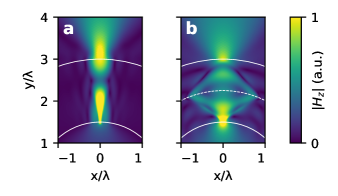
Figure 5: Simulations of a radiation of a point source close to the inner interface imaged by a bright field hyperlens [$\varepsilon_{\theta}=0.2+0.02\mathrm{i}$, $\varepsilon_{r}=-5+2.20\mathrm{i}$], operating in the canalization regime (a). Similar bright-field hyperlens, but using pseudocanalizing structure consisting of two HMM layers [$\varepsilon_{\theta}^{(1)}=1+0.05\mathrm{i}$, $\varepsilon_{r}^{(1)}=-1+0.05\mathrm{i}$, $\varepsilon_{\theta}^{(2)}=\varepsilon_{\theta}^{(1)*}$, $\varepsilon_{r}^{(2)}=\varepsilon_{r}^{(1)*}/2$] (b). For all structures the inner radius is $r_{1}=1.5\lambda$ and the outer radius $r_{2}=3\lambda$. Dashed line in (b) shows split between $\mu$-positive and $\mu$-negative media.

Similar considerations hold for a dark-field hyperlens (based on a type-II HMM): the scaling for the compensation layer follows the same relation [Eq. (25)]. Simulation results for the dark-field hyperlens are shown in Fig. 6: the background radiation is still filtered out (dark-field operation is preserved), while scattered fields from the small dielectric object are passing through the device. As discussed in Section IV, the filtering of low-k waves affects the image so that dark-field operation comes at the cost of image quality. By reducing the low-k cutoff ($k_{c}$) the image quality is improved, as we discussed in case of the flat geometry [see Fig. 4(a)].

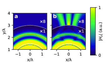
Figure 6: Simulations demonstrating functioning of a dark-field hyperlens with two complementary HMM layers operating in pseudocanalized regime [$\varepsilon_{\theta}^{(1)}=-1+0.05\mathrm{i}$, $\varepsilon_{r}^{(1)}=1+0.05\mathrm{i}$, $\varepsilon_{\theta}^{(2)}=1+0.05\mathrm{i}$, $\varepsilon_{r}^{(2)}=\left(-1+0.05\mathrm{i}\right)/2$, $\mu^{(1)}=1$, $\mu^{(2)}=-1$]. Simulations without (a) and with (b) a small subwavelength scatterer show that the incoming background radiation is filtered, whereas scattered fields from the weakly scattering dielectric object pass through the system.

The hyperlens resolution is determined by two factors: magnification and broadening. The fields on the outer interface should be imaged by far-field optics and hence must be above the diffraction limit. Given hyperlens with magnification $M$ the resolution limit is then $\lambda/2M$. In our case, the hyperlens geometry used has $2\times$ magnification leading to resolution of $\lambda/4$. However, the broadening inside the HMM is also an important consideration: if the beams originating from a point source are broadened too much, they will overlap in the output. In such a case the resolution will be limited by the broadening of the beams. In Fig. 7 we show that both canalizing and pseudocanalizing bright-field hyperlenses have comparable performance in the limiting case of $\lambda/4$ separation. In Fig. 7 we show that both canalizing [Fig. 5(a)] and pseudocanalizing bright-field hyperlens [Fig. 5(b)] have small enough broadening so that the required resolution $\lambda/4$ can be reached. However, for the hyperlens used here, if a better resolution is needed, then losses must be reduced, otherwise the broadening will be a limiting factor.

In Fig. 8(a) we compare the performance of the pseudocanalizing bright-field [Fig. 5(b)] and the dark-field hyperlens (Fig. 6). At the resolution limit the pseudocanalizing dark-field hyperlens offers competitive performance with respect to the bright-field hyperlens. We even see an edge-enhancing behavior associated with high-pass filtering due to filtering low-k waves, which enhances the contrast between the two peaks.

However, as shown in Fig. 8(b) the behavior of a dark-field hyperlens is not straightforward. Although (magnification-limited) resolution of $\lambda/4$ is reached with relative ease, the sidelobes associated with low-k filtering are present and could be problematic for some configurations. In our case, the worst case happens for a source separation of $0.36\lambda$ where the sidelobes of two sources interfere constructively. Nonetheless, here the effect is not strong enough to pose serious problems: the ratio between the main peak and the highest sidelobe is about 1.2. This is comparable to the worst case performance of the bright-field pseudocanalizing hyperlens, shown in Fig. 8(a), where the ratio between the peak and the valley between the peaks is also around 1.2.

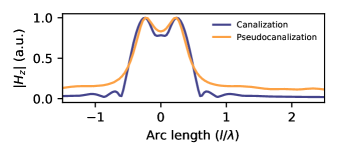
Figure 7: Magnetic field norm along the outer interface of the hyperlens due to two point sources. The two sources near the inner interface are separated by $\lambda/4$. The blue line shows behavior of canalizing bright-field hyperlens [Fig. 5(a)] while the orange line shows the corresponding case for a pseudocanalizing hyperlens [Fig. 5(b)].

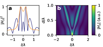
Figure 8: (a) Magnetic field norm along the outer interface of a pseudocanalizing bright-field hyperlens (orange line) and a pseudocanalizing dark-field hyperlens (blue ling). The two point sources are separated by $\lambda/4$. (b) Magnetic field norm along the outer interface as a function of the point source separation $d$. The dotted lines show location of the main peaks from the two point sources.

VI Conclusions

We have shown that the effect of the canalization regime can be understood as propagation of fields without phase accumulation. This suppression of phase term minimizes the signal broadening in the HMM and prevents distortions of the image. We have extended the idea of the canalization regime from homogeneous hyperbolic media to systems consisting of two complementary hyperbolic slabs (pseudocanalizing system), where the phase propagation in the slabs cancels each other so that the propagated fields have no any additional phase term. Unlike a canalizing system, a pseudocanalyzing system allows to sustain the dark-field imaging properties along with the image quality comparable to a canalizing HMM.

This idea of pseudocanalization also applies for cylindrical geometries, i.e. for typical hyperlens designs. Magnification stemming from cylindrical geometry creates some new considerations for the material parameters, but we show that the principle still stands and a pseudocanalizing system performs as well as a the canalizing system. Furthermore, this pseudocanalizing system could be used to improve dark-field hyperlens designs in terms of the image quality.

Appendix A Derivation of the dispersion relation for HMMs

Since the system is invariant in $z$-direction we can effectively consider a two-dimensional case and limit the derivation to TM waves (for TE waves we would end up with isotropic dispersion). The procedure in Ref. Eroglu, 2010 can be followed for general derivation. We start with

$$\mathbf{E} = E_{x}\mathbf{\hat{x}}+E_{y}\hat{\mathbf{y}}\,,$$ (26)

$$\mathbf{H} = H_{z}\hat{\mathbf{z}}\,.$$ (27)

With the help of the constitutive equations we write $\mathbf{D}$ and $\mathbf{B}$ fields as

$$\mathbf{D} = \varepsilon_{0}\left(\varepsilon_{x}E_{x}\mathbf{\hat{x}}+\varepsilon_{y}E_{y}\hat{\mathbf{y}}\right)\,,$$ (28)

$$\mathbf{B} = \mu_{0}\mu H_{z}\hat{\mathbf{z}}\,.$$ (29)

After combining the above relations and (source-free) Maxwell’s curl equations

$$\nabla\times\mathbf{E} = -i\omega\mathbf{B}\,,$$ (30)

$$\nabla\times\mathbf{H} = i\omega\mathbf{D}\,,$$ (31)

and using $\nabla\cdot\mathbf{D}=0$ we end up with (for $i=x,y$)

$$\frac{1}{\varepsilon_{y}}\frac{\partial^{2}E_{i}}{\partial x^{2}}+\frac{1}{\varepsilon_{x}}\frac{\partial^{2}E_{i}}{\partial y^{2}}+\omega^{2}\varepsilon_{0}\mu_{0}\mu E_{i}=0\,.$$ (32)

After substituting the plane wave solution $\mathbf{E}=\mathbf{E}_{0}\exp\left(i\mathbf{k}\cdot\mathbf{r}\right),$ we derive the dispersion equation:

$$k_{x}^{2}/\varepsilon_{y}+k_{y}^{2}/\varepsilon_{x}=\mu\omega^{2}/c^{2}\,.$$ (33)

We point out that the magnetic permeability can be anisotropic [$\hat{\mu}=\mathrm{diag}\left(\mu_{x},\mu_{y},\mu_{z}\right)$], but since one component ($H_{z}$) is nonzero, only $\mu_{z}$ component would enter the dispersion relation for TM waves.

Appendix B Phase accumulation for cylindrical waves

We use Maxwell’s curl equations [Eqs. (30) and (31)] to obtain the wave equation

$$\nabla\times\left(\hat{\varepsilon}^{-1}\nabla\times\mathbf{H}\right)=k_{0}^{2}\mu\mathbf{H}\,,$$ (34)

for which we assume TM fields of form $\mathbf{H}\left(r,\theta\right)=F\left(r\right)\exp\left(im\theta\right)\hat{\mathbf{z}}$. Solving the differential equation yields a general solution for the fields $\mathbf{H}=H_{z}\mathbf{\hat{z}}$ in the form

$$H_{z}\left(r,\theta\right)=\exp\left(im\theta\right)\left[aH_{\nu}^{(1)}\left(k_{r}r\right)+bH_{\nu}^{(2)}\left(k_{r}r\right)\right]\,,$$ (35)

where $\nu=m\cdot\sqrt{\varepsilon_{\theta}/\varepsilon_{r}}$ and $k_{r}=k_{0}\sqrt{\varepsilon_{\theta}}$. The angular momentum mode number $m$ is the number of wavelengths per angle of full rotation ($2\pi$). By analogy with plane waves, it is useful to introduce a tangential wavenumber $k_{\theta}$ (i.e. the number of wavelengths per unit length), which is related to the angular momentum mode number by $m=k_{\theta}r$. As $m$ is fixed for a given wave component, we have $k_{\theta}^{\prime}r_{0}=k_{\theta}r$, from which it follows that

$$k_{\theta}=k_{\theta}^{\prime}\frac{r_{0}}{r}\,,$$ (36)

which shows that the wavevectors are compressed during propagation, corresponding to the magnification of the image.

As for a planar system, the aim here is to obtain expressions for phase accumulation. However, obtaining the analytical expressions in cylindrical basis is not straightforward. Instead we approach the problem with modified plane waves. The key difference between planar and cylindrical geometry is magnification of the image [i.e. scaling of the $k_{\theta},$ given by Eq. (36)]. In planar geometry the phase propagation is expressed with

$$E_{2}=E_{1}\exp\left(ik_{y}\left(x_{2}-x_{1}\right)\right)\,,$$ (37)

where the acquired phase is just $\mathrm{Re}\left(k_{y}\right)\left(x_{2}-x_{1}\right)$. To account for magnification arising from cylindrical geometry we can express the acquired phase by

$$\mathrm{Re}\intop_{r_{1}}^{r_{2}}k_{r}\left(r\right)\,dr\,.$$ (38)

In our case $k_{r}$ is the propagation constant and a function of $r$ (via $k_{\theta}$). The propagation constant $k_{y}$ is given by Eq. (5), however here $k_{x}$ is scaled as given by Eq. (36). As shown in Fig. 9, this approach of using plane waves with scaled $k_{\theta}$ manages to capture the phase accumulation effects in cylindrical geometry. Unlike solution in cylindrical basis, this approach allows for analytical integration of Eq. (38).

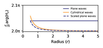
Figure 9: Acquired phase per distance ($\frac{d}{dr}\mathrm{arg}\,H_{z}$). For plane waves (solid blue line) the phase is linearly dependent on propagated distance [$\mathrm{arg}\,H_{z}=k_{y}\left(x_{2}-x_{1}\right)$]. However, in cylindrical geometry the phase propagation is not linear — as seen for Hankel waves (solid yellow line) the phase propagation depends on the propagation distance. Dashed blue line shows phase propagation using scaled plane waves [Eq. (38)], which offers a good approximation for cylindrical waves.

We anticipate that the material parameters of the second medium must be scaled to counteract the effect of magnification. We note that compression of dispersion relation [Eq. (4)] in $k_{\theta}$ direction is achieved by scaling $\varepsilon_{r}$. Therefore we alter the second medium as follows: $\varepsilon_{r}^{(2)}=\varepsilon_{r}^{\prime(2)}/\xi$.

Integration of Eq. (38) can be carried out analytically, resulting in an analytical expression for the total acquired phase as a function of the wavevector $k_{\theta}$, geometric magnification factor $M=1+h/r_{1}$ (where $r_{1}$ is the inner radius and $h$ is the hyperlens thickness) and scaling parameter $\xi$. Taking the limit $k_{\theta}\to\infty$ allows us to obtain a simple expression for material scaling:

$$\xi=\left\{\ln\left[\left(M+1\right)^{2}/4\right]/\ln\left[\left(M+1\right)^{2}/4M^{2}\right]\right\}^{2}\,.$$ (39)

For small magnification factors (i.e. $h\sim r_{1}$ ) the expression further simplifies to

$$\xi\approx M\,.$$ (40)

It is easy to verify that the resulting expression [Eq. (40)] is a good approximation for our geometry. Furthermore, we numerically verified that the resulting scaling parameter is the optimal choice when operating in a proper cylindrical basis using Hankel functions [Eq. (35)].

References

- Dunn (1999) R. C. Dunn, Chemical Reviews 99, 2891 (1999).
- Hell and Wichmann (1994) S. W. Hell and J. Wichmann, Optics Letters 19, 780 (1994).
- Klar and Hell (1999) T. A. Klar and S. W. Hell, Optics Letters 24, 954 (1999).
- Pendry (2000) J. B. Pendry, Physical Review Letters 85, 3966 (2000).
- Jacob et al. (2006) Z. Jacob, L. V. Alekseyev, and E. Narimanov, Optics Express 14, 8247 (2006).
- Liu et al. (2007) Z. Liu, H. Lee, Y. Xiong, C. Sun, and X. Zhang, Science 315, 1686 (2007).
- Yao et al. (2008) J. Yao, Z. Liu, Y. Liu, Y. Wang, C. Sun, G. Bartal, A. M. Stacy, and X. Zhang, Science 321, 930 (2008).
- Valentine et al. (2008) J. Valentine, S. Zhang, T. Zentgraf, E. Ulin-Avila, D. A. Genov, G. Bartal, and X. Zhang, Nature 455, 376 (2008).
- Smith and Schurig (2003) D. R. Smith and D. Schurig, Physical Review Letters 90, 077405 (2003).
- Liu et al. (2008) Y. Liu, G. Bartal, and X. Zhang, Optics Express 16, 15439 (2008).
- Poddubny et al. (2013) A. Poddubny, I. Iorsh, P. Belov, and Y. Kivshar, Nature Photonics 7, 948 (2013).
- Novotny and Hecht (2006) L. Novotny and B. Hecht, Principles of Nano-Optics (Cambridge University Press, 2006).
- Lu and Liu (2012) D. Lu and Z. Liu, Nature Communications 3, 1205 (2012).
- Xiong et al. (2009) Y. Xiong, Z. Liu, and X. Zhang, Applied Physics Letters 94, 203108 (2009).
- Ikonen et al. (2007) P. Ikonen, C. Simovski, S. Tretyakov, P. Belov, and Y. Hao, Applied Physics Letters 91, 104102 (2007).
- Rho et al. (2010) J. Rho, Z. Ye, Y. Xiong, X. Yin, Z. Liu, H. Choi, G. Bartal, and X. Zhang, Nature Communications 1, 143 (2010).
- Benisty and Goudail (2012) H. Benisty and F. Goudail, Journal of the Optical Society of America B 29, 2595 (2012).
- Repän et al. (2015) T. Repän, A. V. Lavrinenko, and S. V. Zhukovsky, Optics Express 23, 25350 (2015).
- Alu and Engheta (2003) A. Alu and N. Engheta, IEEE Transactions on Antennas and Propagation 51, 2558 (2003).
- Shekhar et al. (2014) P. Shekhar, J. Atkinson, and Z. Jacob, Nano Convergence 1, 14 (2014).
- Belov et al. (2006) P. A. Belov, Y. Hao, and S. Sudhakaran, Physical Review B 73, 033108 (2006).
- Salandrino and Engheta (2006) A. Salandrino and N. Engheta, Physical Review B 74, 075103 (2006).
- Jacob et al. (2007) Z. Jacob, L. V. Alekseyev, and E. Narimanov, Journal of the Optical Society of America A 24, A52 (2007).
- Lee et al. (2007) H. Lee, Z. Liu, Y. Xiong, C. Sun, and X. Zhang, Optics Express 15, 15886 (2007).
- Castaldi et al. (2012) G. Castaldi, S. Savoia, V. Galdi, A. Alù, and N. Engheta, Physical Review B 86, 115123 (2012).
- Eroglu (2010) A. Eroglu, Wave Propagation and Radiation in Gyrotropic and Anisotropic Media (Springer, 2010).