Abstract

We derive a positivity bound on the right-chiral tensor coupling $\mathop{\rm Im}\nolimits g_{R}$ in polarized top quark decay by analyzing the angular decay distribution of the three-body polarized top quark decay $t(\uparrow)\to b+\ell^{+}+\nu_{\ell}$ in next-to-leading order QCD. We obtain the bound $-0.0420\leq\mathop{\rm Im}\nolimits g_{R}\leq 0.0420$.

The general matrix element for the decay $t\to b+W^{+}$ including the leading order (LO) standard model (SM) contribution is usually written as (see e.g. Ref. [1])

$$M_{tbW^{+}}=-\frac{g_{W}}{\sqrt{2}}\varepsilon^{\mu\,\ast}\bar{u}_{b}\Big{[}(V^{\ast}_{tb}+f_{L})\gamma_{\mu}P_{L}+f_{R}\gamma_{\mu}P_{R}+\frac{i\sigma_{\mu\nu}\,q^{\nu}}{m_{W}}\Big{(}g_{L}\,P_{L}+g_{R}\,P_{R}\Big{)}\Big{]},$$ (1)

where $P_{L,R}=(1\mp\gamma_{5})/2$. The SM structure of the $tbW^{+}$ vertex is obtained by dropping all terms except for the contribution proportional to $V^{\ast}_{tb}\sim 1$.

The angular decay distribution for polarized top quark decay $t(\uparrow)\to b+\ell^{+}+\nu_{\ell}$ in the top quark rest frame is given by

$$\frac{d\Gamma}{d\cos\theta d\phi} = A+BP_{t}\cos\theta_{P}+CP_{t}\sin\theta_{P}\cos\phi+DP_{t}\sin\theta_{P}\sin\phi$$ (2)

which corresponds to the decay distribution introduced in Refs. [2, 3] augmented by the last $T$-odd term. At LO of the SM one has $A=B$ and $C=D=0$. The second azimuthal term proportional to $D$ corresponds to a $T$-odd contribution. This can be seen by rewriting the angular factor as a triple product according to

$$\sin\theta_{P}\sin\phi=\hat{p}_{\ell}\cdot(\hat{p}_{b}\times\hat{s}_{t})$$ (3)

where (see Fig. 1)

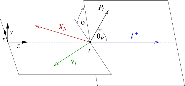
Figure 1: Definitions of polar and azimuthal angles for the process $t\to b+W^{+}(\to\ell^{+}+\nu_{\ell})$

$$\hat{p}_{\ell}=(0,0,1)\qquad\hat{p}_{b}=(\sin\theta_{b},0,\cos\theta_{b})\qquad\hat{s}_{t}=(\sin\theta_{P}\cos\phi,\cos\theta_{P}\sin\phi,\cos\theta_{P})$$ (4)

Let us repeat the arguments presented in Ref. [3] that led us to the conclusion that the equality $A=B$ already implies the vanishing of the $T$-even azimuthal contribution $C$ confirming the LO result $C=0$. Consider Eq. (2) for $P_{t}=1$ and $\sin\phi=0$, i.e. $\cos\phi=\pm 1$. Then factor out the unpolarized rate term $A$. Assume first that $C/A$ is positive and choose $\cos\phi=-1$. Expand the trigonometric functions around $\theta_{P}=\pi$ for positive values of $\delta$, i.e. $\cos(\pi-\delta)\approx-1+\frac{1}{2}\delta^{2}$ and $\sin(\pi-\delta)\approx\delta$. The differential rate is then proportional to

$$1+\cos\theta_{P}-\frac{C}{A}\sin\theta_{P}\approx\frac{1}{2}\delta^{2}-\frac{C}{A}\delta=\frac{1}{2}\delta\left(\delta-\frac{2C}{A}\right).$$ (5)

The differential rate can be seen to be negative for $\delta$ in the interval $[0,2C/A]$. The interval can be shrunk to zero by setting $2C/A=0$, i.e. by setting $C=0$. If $C/A$ is assumed to be negative, one chooses $\cos\phi=+1$ and again arrives at the conclusion $2C/A=0$ by expanding the trigonometric functions around $\theta_{P}=\pi$.

The same chain of arguments but this time with $\cos\phi=0$ leads to the LO positivity constraint for the $T$-odd structure, $D=0$.

At next-to-leading order (NLO) of QCD one no longer has $A=B$. However, the relative difference $(A-B)/A$ is quite small which, as we will see, in turn implies useful positivity constraints for the $T$-odd structure coefficient $D$. As concerns the $T$-even azimuthal structure, the NLO corrections to the LO result $C=0$ are so small that the positivity of the differential rate is not endangered [3].

We now derive the NLO positivity constraint for the $T$-odd structure coefficient $D$. We shall work in the approximation $m_{b}=0$ which implies that the coupling terms $f_{R}$ and $g_{L}$ in Eq. (1) are zero. The NLO forms of the integrated $m_{b}=0$ rates are listed in Refs. [4, 5, 6]. They read

$$\frac{d\Gamma}{d\cos\theta d\phi} = (A^{(0)}+A^{(1)})\Big{(}1+\frac{A^{(0)}+B^{(1)}}{A^{(0)}+A^{(1)}}P_{t}\cos\theta_{P}$$ (6)

$$+\frac{C}{A^{(0)}+A^{(1)}}P_{t}\sin\theta_{P}\cos\phi+\frac{D}{A^{(0)}+A^{(1)}}P_{t}\sin\theta_{P}\sin\phi\Big{)},$$

where

$$\frac{A^{(1)}}{A^{(0)}} = \frac{\alpha_{s}C_{F}}{4\pi}\,\frac{1}{(1-x^{2})^{2}(1+2x^{2})}\bigg{(}(1-x^{2})(5+9x^{2}-6x^{4})$$ (7)

$$-2(1-x^{2})^{2}(1+2x^{2})\Big{[}\frac{2\pi^{2}}{3}+4\ln(1-x^{2})\ln x+4\mathop{\rm Li}\nolimits_{2}(x^{2})\Big{]}$$

$$-8x^{2}(1+x^{2})(1-2x^{2})\ln x-2(1-x^{2})^{2}(5+4x^{2})\ln(1-x^{2})\bigg{)}$$

$$= -0.0846955,$$

and

$$\frac{B^{(1)}}{A^{(0)}} = \frac{\alpha_{s}C_{F}}{4\pi}\,\frac{1}{(1-x^{2})^{2}(1+2x^{2})}\bigg{(}-(1-x^{2})(15-x^{2}+2x^{4})$$ (8)

$$+(1-x^{2})(1+x^{2}+4x^{4})\frac{2\pi^{2}}{3}-2(1-x^{2})^{2}(5+4x^{2})\ln(1-x^{2})$$

$$-16x^{2}(2+x^{2}-x^{4})\ln x-16(1-x^{2})(2+2x^{2}-x^{4})\ln x\ln(1-x^{2})$$

$$-4(1-x^{2})(5+5x^{2}-4x^{4})\mathop{\rm Li}\nolimits_{2}(x^{2})\bigg{)}$$

$$= -0.0863048,$$

where $x=m_{W}/m_{t}$. Here we have also listed the numerical values for the two ratios using $\alpha_{s}(m_{t})=0.1062$, $m_{t}=173.21{\rm\,GeV}$ and $m_{W}=80.385{\rm\,GeV}$ [7]. The ratio expressions $A^{(1)}/A^{(0)}$ and $B^{(1)}/A^{(0)}$ have been rechecked in Ref. [3]. Reference [3] also contains results on the azimuthal rate coefficient $C$. This coefficient, however, will be of no concern in the derivation of the positivity bounds for the $T$-odd rate coefficient $D$. In fact, setting $sin\phi=\pm 1$ will eliminate the contribution of $C$. This will be our choice.

Next we must determine the contribution of the imaginary part of the coupling factor $g_{R}$ to the $T$-odd azimuthal rate term $D$. The relevant contribution arises from the interference of the coupling factor $g_{R}$ with the Born term contribution. It is for this reason that there is no $\mathop{\rm Im}\nolimits f_{L}$ contribution to the $T$-odd rate coefficient $D$ since the coupling term is self-interfering. After some algebra one finds

$$\frac{D}{A^{(0)}}=\frac{3\pi(1-x^{2})}{4(1+2x^{2})}\mathop{\rm Im}\nolimits g_{R}$$ (9)

where we have only kept the contribution linear in $\mathop{\rm Im}\nolimits g_{R}$. Further, we assume $\mathop{\rm Im}\nolimits g_{R}$ to be positive, and set $P_{t}=1$ and $\sin\phi=-1$. We expand around $\theta_{P}=\pi$ for small positive values of $\delta$ which gives $\cos(\pi-\delta)=-1+\frac{1}{2}\delta^{2}$ and $\sin(\pi-\delta)=\delta$ to obtain

$$W(\theta_{P})\sim 1+(1-\Delta)\cos\theta_{P}-\frac{D}{A^{(0)}+A^{(1)}}\sin\theta_{P}=\Delta-\frac{D\delta}{A^{(0)}+A^{(1)}}+\frac{1-\Delta}{2}\delta^{2},$$ (10)

where we have defined the small quantity

$$\Delta=\frac{A^{\rm NLO}-B^{\rm NLO}}{A^{\rm NLO}}=\frac{A^{(1)}-B^{(1)}}{A^{(0)}+A^{(1)}}=\frac{A^{(1)}-B^{(1)}}{A^{(0)}(1+A^{(1)}/A^{(0)})},$$ (11)

keeping in mind that $A^{(0)}=B^{(0)}$. Numerically one has $\Delta=0.001758$ where the small difference to the numerical results in Ref. [3] results from having used updated values $m_{W}=80.385{\rm\,GeV}$ and $m_{t}=173.21{\rm\,GeV}$ [7].

The rate proportional to $W(\theta_{P})$ in Eq. (10) becomes negative if the contribution proportional to $\mathop{\rm Im}\nolimits g_{R}$ becomes larger than the remaining terms. However, this is no longer the case if the quadratic equation (10) in $\delta$ has no real-valued zeros. The pertinent condition for the discriminant reads

$$\frac{3\pi(1-x^{2})}{4(1+2x^{2})}|\mathop{\rm Im}\nolimits g_{R}|\leq\sqrt{2\Delta(1-\Delta)}\left(1+\frac{A^{(1)}}{A^{(0)}}\right).$$ (12)

Numerically one obtains

$$\mathop{\rm Im}\nolimits g_{R}\leq\,0.0420$$ (13)

The same chain of arguments, but now for negative values of $\mathop{\rm Im}\nolimits g_{R}$ and $\sin\phi=1$ leads to $\mathop{\rm Im}\nolimits g_{R}\geq\,-0.0420$ such that one has the two-sided constraint

$$\mathop{\rm Im}\nolimits g_{R}\in[-0.0420,\,0.0420]\,.$$ (14)

The angle $\delta_{0}$ for which the quadratic form (10) becomes degenerate can be calculated to be $\delta_{0}=\sqrt{2\Delta/(1-\Delta)}=\pm 0.0593$. The corrections to the expansion of $\cos(\pi-\delta)$ and $\sin(\pi-\delta)$ are of the order $O(\delta^{2}=0.00352)$ and, therefore, quite small.

In Ref. [8] we have calculated the SM absorptive electroweak contributions to $\mathop{\rm Im}\nolimits g_{R}$ with the result $\mathop{\rm Im}\nolimits g_{R}=-2.175\times 10^{-3}$ (see also Refs. [9, 10]). This value is easily accommodated in the positivity bound (14).

The ATLAS Collaboration has recently published the bound [11]

$$\mathop{\rm Im}\nolimits g_{R}\in[-0.18,\,0.06]$$ (15)

based on the analysis of sequential polarized two-body top quark decays $t(\uparrow)\to b+W^{+}(\to\ell^{+}+\nu)$. A somewhat tighter bound has been published in Ref. [12] using also sequential polarized two-body top quark decays. The bound reads

$$\mathop{\rm Im}\nolimits\left(\frac{g_{R}}{f_{L}}\right)\in[-0.07,\,0.06]$$ (16)

which we translate into a bound on $\mathop{\rm Im}\nolimits g_{R}$ by substituting the LO result $f_{L}=1$ in Eq. (16). Both bounds are not far away from the positivity bound on $\mathop{\rm Im}\nolimits g_{R}$ derived in this paper. Using the same chain of arguments one can establish the corresponding bound for $m_{b}\neq 0$. Using NLO $m_{b}\neq 0$ results from Ref. [6] on the unpolarized and polarized rate functions $A^{(1)}$ and $B^{(1)}$ we find that for $m_{b}=4.8{\rm\,GeV}$ the bound is marginally strengthened to $\mathop{\rm Im}\nolimits g_{R}\in[-0.0418,0.0418]$. The condition for obtaining this bound reads

$$\frac{3\pi(1-x^{2}+y^{2})\sqrt{\lambda}}{4\left(\lambda+3x^{2}(1-x^{2}+y^{2})\right)}|\mathop{\rm Im}\nolimits g_{R}|\leq\sqrt{2\Delta(1-\Delta)}\left(1+\frac{A^{(1)}}{A^{(0)}}\right),$$ (17)

where $y=m_{b}/m_{t}$ and $\lambda=\lambda(1,x^{2},y^{2})=1+x^{4}+y^{4}-2x^{2}-2y^{2}-2x^{2}y^{2}$ is the Källén function. $A^{(0)}$, $A^{(1)}$ and the small quantity $\Delta$ are evaluated for $m_{b}\neq 0$.

References

• [1] W.ย Bernreuther, P.ย Gonzalez and M.ย Wiebusch, Eur.ย Phys.ย J.ย C60 (2009) 197
• [2] J.G.ย Kรถrner and D.ย Pirjol, Phys.ย Rev.ย D60 (1999) 014021
• [3] S.ย Groote, W.S.ย Huo, A.ย Kadeer and J.G.ย Kรถrner, Phys.ย Rev.ย D76 (2007) 014012
• [4] A.ย Czarnecki, M.ย Jeลผabek and J.H.ย Kรผhn, Nucl.ย Phys.ย B351 (1991) 70
• [5] A.ย Czarnecki, M.ย Jeลผabek, J.G.ย Kรถrner and J.H.ย Kรผhn,
Phys.ย Rev.ย Lett.ย 73 (1994) 384
• [6] A.ย Czarnecki and M.ย Jeลผabek, Nucl.ย Phys.ย B427 (1994) 3
• [7] C.ย Patrignani et al. [Particle Data Group], Chin.ย Phys.ย C40 (2016) 100001
• [8] M.ย Fischer, S.ย Groote and J.G.ย Kรถrner,
$T$-odd correlations in polarized top quark decays $t(\uparrow)\to X_{b}+W^{+}(\to\ell^{+}+\nu_{\ell})$ from one-loop electroweak correctionsโ€, in preparation
• [9] G.A.ย Gonzalez-Sprinberg, R.ย Martinez and J.ย Vidal,
JHEP 07 (2011) 094; Erratum: [JHEP 05 (2013) 117]
• [10] A.ย Arhrib and A.ย Jueid, JHEP 08 (2016) 082
• [11] M.ย Aaboud et al. [ATLAS Collaboration], JHEP 04 (2017) 124
• [12] M.ย Aaboud et al. [ATLAS Collaboration], JHEP 1712 (2017) 017