New insights in the mid-infrared bubble N49 site: a clue of collision of filamentary molecular clouds

Abstract

We investigate the star formation processes operating in a mid-infrared bubble N49 site, which harbors an O-type star in its interior, an ultracompact H ii region, and a 6.7 GHz methanol maser at its edges. The ¹³CO line data reveal two velocity components (at velocity peaks $\sim$88 and $\sim$95 km s^-1) in the direction of the bubble. An elongated filamentary feature (length $>$15 pc) is investigated in each molecular cloud component, and the bubble is found at the interface of these two filamentary molecular clouds. The Herschel temperature map traces all these structures in a temperature range of $\sim$16–24 K. In the velocity space of ¹³CO, the two molecular clouds are separated by $\sim$7 km s^-1, and are interconnected by a lower intensity intermediate velocity emission (i.e. a broad bridge feature). A possible complementary molecular pair at [87, 88] km s^-1 and [95, 96] km s^-1 is also observed in the velocity channel maps. These observational signatures are in agreement with the outcomes of simulations of the cloud-cloud collision process. There are also noticeable embedded protostars and Herschel clumps distributed toward the filamentary features including the intersection zone of the two molecular clouds. In the bubble site, different early evolutionary stages of massive star formation are also present. Together, these observational results suggest that in the bubble N49 site, the collision of the filamentary molecular clouds appears to be operated about 0.7 Myr ago, and may have triggered the formation of embedded protostars and massive stars.

1. Introduction

Massive stars ($\geq$ 8 M_⊙) can inject large amounts of energy to the neighboring interstellar medium (ISM), hence these stars can trigger the birth of a new generation of stars including young massive star(s) (Deharveng et al., 2010). However, the formation mechanisms of massive stars and their feedback processes are still being debated (Zinnecker & Yorke, 2007; Tan et al., 2014). In recent years, the theoretical and observational studies of the cloud-cloud collision (CCC) process have drawn considerable attention, which can produce massive OB stars and young stellar clusters at the junction of molecular clouds (e.g., Habe & Ohta, 1992; Furukawa et al., 2009; Anathpindika, 2010; Ohama et al., 2010; Inoue & Fukui, 2013; Takahira et al., 2014; Fukui et al., 2014, 2016; Torii et al., 2015, 2017; Haworth et al., 2015a, b; Dewangan, 2017a; Dewangan & Ojha, 2017b). Torii et al. (2017) suggested that the onset of the CCC process in a given star-forming region could be observationally inferred through the detection of a bridge feature connecting the two clouds in velocity space, the broad CO line wing in the intersection of the two clouds, and the complementary distribution of the two colliding clouds. However, such observational investigation is still limited in the literature (e.g. Torii et al., 2017).

The mid-infrared (MIR) bubble, N49 (l = 028$\arcdeg$.827; b = $-$00$\arcdeg$.229; Churchwell et al., 2006) is a very well studied star-forming site containing an H ii region (Watson et al., 2008; Anderson & Bania, 2009; Deharveng et al., 2010; Everett & Churchwell, 2010; Zavagno et al., 2010; Dirienzo et al., 2012). The N49 H ii region is ionized by an O type star (Watson et al., 2008; Deharveng et al., 2010; Dirienzo et al., 2012) and is situated at a distance of 5.07 kpc (Dirienzo et al., 2012). We have also adopted a distance of 5.07 kpc to the bubble N49 throughout the present work. The bubble N49 is classified as a complete or closed ring with an average radius and thickness of 1$\farcm$32 (or 1.95 pc) and 0$\farcm$32 (or 0.45 pc), respectively (Churchwell et al., 2006). Dirienzo et al. (2012) examined the ¹³CO line data and suggested the presence of two velocity components (at $\sim$87 and $\sim$95 km s^-1) in the direction of the bubble. Based on the radio recombination line observations, the velocity of the ionized gas in the N49 H ii region was reported to be $\sim$90.6 km s^-1 (Anderson & Bania, 2009). Using the APEX 870 $\mu$m dust continuum data, Deharveng et al. (2010) reported the detection of at least four massive clumps (M_clump $\sim$ 190–2300 M_⊙) toward the infrared rim of the bubble (see Figure 18 in Deharveng et al. (2010) and also Figure 1 in Zavagno et al. (2010)). An ultracompact (UC) H ii region and a 6.7 GHz methanol maser emission (MME) (velocity range $\sim$79.4–92.7 km s^-1; Walsh et al., 1998; Szymczak et al., 2012) are also detected toward the dust condensations, which are seen at the edges of the bubble (e.g. Deharveng et al., 2010; Zavagno et al., 2010; Dirienzo et al., 2012). The bubble N49 has also been considered as a candidate of a wind-blown bubble (Everett & Churchwell, 2010). Using the multi-wavelength data, previous studies suggested that the N49 H ii region is interacting with its surrounding molecular cloud, and has been cited as a possible site of triggered star formation (Watson et al., 2008; Anderson & Bania, 2009; Zavagno et al., 2010; Deharveng et al., 2010; Dirienzo et al., 2012).

Despite the availability of several observational data sets, the knowledge of the physical environments over larger spatial scale around the bubble is still unknown. Furthermore, the study of an interaction between molecular cloud components is yet to be performed in the bubble N49 site. To study the physical environment and star formation processes around the bubble N49, we revisit the bubble using multi-wavelength data covering from the radio to near-infrared (NIR) wavelengths. Such analysis offers an opportunity to examine the distribution of dust temperature, column density, extinction, ionized emission, kinematics of molecular gas, and young stellar objects (YSOs).

The paper is arranged in the following way. The details of the adopted data sets are described in Section 2. Section 3 gives the outcomes concerning to the physical environment and point-like sources. In Section 4, we present the possible star formation processes ongoing in our selected target region. Finally, Section 5 summarizes the main results.

2. Data sets and analysis

In this paper, we have chosen a field of $\sim$0$\arcdeg$.42 $\times$ 0$\arcdeg$.42 ($\sim$37.2 pc $\times$ 37.2 pc; centered at $l$ = 28$\arcdeg$.844; $b$ = $-$0$\arcdeg$.220) around the MIR bubble N49 site. In the following, we provide a brief description of the adopted multi-wavelength data.

2.1. Radio Centimeter Continuum Map

Radio continuum map at 20 cm was obtained from the VLA Multi-Array Galactic Plane Imaging Survey (MAGPIS; Helfand et al., 2006). The MAGPIS 20 cm map has a 6$\farcs$2 $\times$ 5$\farcs$4 beam size and a pixel scale of 2$\arcsec$/pixel.

2.2. ¹³CO (J=1$-$0) Line Data

In order to examine the molecular gas associated with the selected target, the Galactic Ring Survey (GRS; Jackson et al., 2006) ¹³CO (J=1$-$0) line data were adopted. The GRS line data have a velocity resolution of 0.21 km s^-1, an angular resolution of 45$\arcsec$ with 22$\arcsec$ sampling, a main beam efficiency ($\eta_{\rm mb}$) of $\sim$0.48, a velocity coverage of $-$5 to 135 km s^-1, and a typical rms sensitivity (1$\sigma$) of $\approx 0.13$ K (Jackson et al., 2006).

2.3. Far-infrared and Sub-millimeter Data

We examined the far-infrared (FIR) and sub-millimeter (mm) images downloaded from the Herschel Space Observatory (Pilbratt et al., 2010; Poglitsch et al., 2010; Griffin et al., 2010; de Graauw et al., 2010) data archives. Level2_-5 processed 160–500 $\mu$m images were retrieved through the Herschel Interactive Processing Environment (HIPE, Ott, 2010). The beam sizes of the Herschel images are 5$\farcs$8, 12$\arcsec$, 18$\arcsec$, 25$\arcsec$, and 37$\arcsec$ for 70, 160, 250, 350, and 500 $\mu$m, respectively (Poglitsch et al., 2010; Griffin et al., 2010). The plate scales of 70, 160, 250, 350, and 500 $\mu$m images are 3^′′.2, 3^′′.2, 6^′′, 10^′′, and 14^′′ pixel^-1, respectively. The Herschel images at 250–500 $\mu$m are calibrated in units of surface brightness, MJy sr^-1, while the units of images at 70–160 $\mu$m are Jy pixel^-1.

The sub-mm continuum map at 870 $\mu$m (beam size $\sim$19$\farcs$2) was also retrieved from the APEX Telescope Large Area Survey of the Galaxy (ATLASGAL; Schuller et al., 2009).

2.4. Spitzer and WISE Data

The photometric images and magnitudes of point sources at 3.6–8.0 $\mu$m were downloaded from the Spitzer Galactic Legacy Infrared Mid-Plane Survey Extraordinaire (GLIMPSE; Benjamin et al., 2003) survey (resolution $\sim$2$\arcsec$). In this work, we used the GLIMPSE-I Spring ’07 highly reliable photometric catalog.

We also utilized the Wide Field Infrared Survey Explorer (WISE; Wright et al. (2010)) image at 12 $\mu$m (spatial resolution $\sim$6$\arcsec$) and the Spitzer MIPS Inner Galactic Plane Survey (MIPSGAL; Carey et al., 2005) 24 $\mu$m image (spatial resolution $\sim$6$\arcsec$). Furthermore, the photometric magnitudes of point sources at MIPSGAL 24 $\mu$m (from Gutermuth & Heyer, 2015) were also collected.

3. Results

3.1. MIR bubble N49 and filamentary features

In this section, we present multi-wavelength data to explore the physical environments over larger spatial scale around the bubble N49. Figure 1a shows a color-composite map obtained using the Herschel images (i.e. 250 $\mu$m (red), 160 $\mu$m (green), and 70 $\mu$m (blue)). The MIR bubble N49 is prominently seen in the composite map within a spatial area of 6.5 pc $\times$ 6.5 pc, and the Herschel images also reveal embedded filamentary features (i.e. fl-1, fl-2, and fl-3) in our selected field (see arrows in Figure 1a). We also find that the bubble appears at the junction of filamentary features. However, one cannot confirm the physical association between the bubble and filamentary features without knowledge of velocities of molecular gas. In Figure 1b, we present the observed ¹³CO (J=1–0) profile in the direction of “zone I” (see a highlighted box in Figure 1a), which encompasses spatially some parts of the bubble and the filamentary features. The spectrum is obtained by averaging the “zone I” area, and reveals the presence of at least three velocity components (at peaks around 88, 95, and 100 km s^-1) along the line of sight. Based on the ¹³CO spectrum, in Figures 2a and 2b, we present the overlay of the ¹³CO emissions on the Herschel 350 $\mu$m image. In Figure 2a, the ¹³CO gas is integrated over a velocity range of 83–91 km s^-1, and a majority of molecular gas are found toward the bubble and the filamentary feature “fl-1”. The distribution of molecular gases linked with two other molecular cloud components is presented in Figure 2b. The molecular cloud linked with the filamentary feature “fl-2” is traced in a velocity range of 92–98.8 km s^-1, while the molecular cloud associated with the filamentary feature “fl-3” is depicted in a velocity range of 99–104 km s^-1.

Figure 2c displays the Herschel 350 $\mu$m image overlaid with the MAGPIS 20 cm emission. The ionized emission traced in the MAGPIS map is exclusively seen toward the bubble N49. In Figure 2d, the ATLASGAL 870 $\mu$m continuum map is also superimposed with the 870 $\mu$m emission contour, indicating the presence of several condensations toward the filamentary features and the edges of the bubble. In Figures 2c and 2d, despite the difference in spatial resolution, one can infer that the emission traced in the Herschel 350 $\mu$m is found to be more prominent compared to the emission detected in the 870 $\mu$m continuum map. It has also been reported that space-based Herschel observations could be considered as almost no loss of large-scale emission with respect to the ground-based APEX dust continuum observations (e.g. Liu et al., 2017). In our selected target field, based on the distribution of molecular gas, Figure 3 spatially delineates different elongated filamentary molecular clouds (lengths $\sim$10–19 pc; average widths $\sim$2 pc).

Figure 4 shows a zoomed-in view of the bubble N49 using multi-wavelength images (e.g. Spitzer 8–24 $\mu$m, WISE 12 $\mu$m, Herschel 70–500 $\mu$m, ATLASGAL 870 $\mu$m, GRS ¹³CO, and MAGPIS 20 cm). These images reveal a complete or closed ring morphology, containing the ionized emission in the bubble interior (e.g. Watson et al., 2008; Zavagno et al., 2010). As mentioned before, the N49 H ii region is powered by an O type star (Watson et al., 2008; Deharveng et al., 2010; Dirienzo et al., 2012). Furthermore, a double shell-like structure is also observed in the 12-70 $\mu$m and 20 cm maps (e.g. Watson et al., 2008). The 6.7 GHz MME and the UCH ii region are seen at the edges of the bubble. The UCH ii region was reported to be ionized by a B0V star (e.g. Deharveng et al., 2010). In the panels “j” and “k”, one can also find the presence of two molecular cloud components in the direction of the bubble (e.g. Dirienzo et al., 2012). In Figure 5a, we present a color-composite map produced using the MIR and FIR images (i.e. 70 $\mu$m (red), 24 $\mu$m (green), and 12 $\mu$m (blue)). The composite map is also overlaid with the MAGPIS 20 cm continuum emission, depicting the double shell-like structure. In the composite map, we have also highlighted the previously known UCH ii region and two embedded YSOs (i.e. YSO #1 and YSO#3; see Figure 1 in Zavagno et al. (2010)). Interestingly, the position of the 6.7 GHz MME spatially coincides with the position of the YSO#3 that can be considered as an infrared counterpart (IRc) of the 6.7 GHz MME. No radio cm emission is detected toward the YSO#3. Considering the 6.7 GHz MME as a reliable tracer of a massive YSO (MYSO) (e.g. Walsh et al., 1998; Urquhart et al., 2013), the YSO#3 could be a MYSO candidate at its early formation stage prior to the UCH ii phase. Based on the high resolution 6.7 GHz MME observations, Cyganowski et al. (2009) proposed the presence of a rotating disk associated with YSO#3.

Together, the bubble N49 is a very promising site, where different early evolutionary stages of massive star formation are present.

3.2. Kinematics of molecular gas

In this section, we present a kinematic analysis of the molecular gas in our selected field. In Figure 5b, we show the observed ¹³CO (J=1–0) spectrum in the direction of “Reg 1” (see a solid box in Figure 5a). The spectrum is computed by averaging the area “Reg 1” marked in Figure 5a. In the spectrum, an almost flattened profile is observed between two velocity peaks (or molecular cloud components), which can be referred to as a bridge feature at the intermediate velocity range. This particular outcome indicates a signature of collisions between molecular clouds (Takahira et al., 2014; Haworth et al., 2015a, b; Torii et al., 2017; Bisbas et al., 2017). In other words, it also suggests a mutual interaction of clouds (e.g. Bisbas et al., 2017).

In Figure 6, we display the integrated GRS ¹³CO (J=1$-$0) velocity channel maps (starting from 81 km s^-1 at intervals of 1 km s^-1), tracing three molecular components along the line of sight (also see Figure 3). To further examine the molecular gas distribution in the direction of our selected target field, in Figure 7, we show the integrated ¹³CO intensity map and the position-velocity maps. The integrated GRS ¹³CO intensity map is shown in Figure 7a, where the molecular emission is integrated over 83 to 104 km s^-1. The Galactic position-velocity diagrams of the ¹³CO emission also reveal three velocity components and the noticeable velocity spread (see Figures 7b and 7d). In the velocity space, we find a red-shifted peak (at $\sim$95 km s^-1) and a blue-shifted peak (at $\sim$88 km s^-1) that are interconnected by a lower intensity intermediate velocity emission, suggesting the presence of a broad bridge feature (also see Figure 5b). Figure 7c shows the spatial distribution of three molecular components, similar to those shown in Figures 2a and 2b.

Together, molecular line data confirm that the bubble N49 is found in the intersection of two molecular clouds. The analysis of ¹³CO data also gives an observational clue of the signature of the interaction between molecular cloud components in the bubble site. The implication of these outcomes is presented in more detail in the discussion Section 4.

3.3. Herschel temperature and column density maps

In this section, we present Herschel temperature and column density maps of the bubble N49. Following the methods described in Mallick et al. (2015), these maps are produced from a pixel-by-pixel spectral energy distribution (SED) fit with a modified blackbody to the cold dust emission at Herschel 160–500 $\mu$m (also see Dewangan et al., 2015). In the following, a brief step-by-step explanation of the adopted procedures is provided.

Before the SED fitting process, using the task “Convert Image Unit” available in the HIPE software, we converted the surface brightness unit of 250–500 $\mu$m images to Jy pixel^-1, same as the unit of 160 $\mu$m image. Next, using the plug-in “Photometric Convolution” available in the HIPE software, the 160–350 $\mu$m images were convolved to the angular resolution of the 500 $\mu$m image ($\sim$37$\arcsec$), and then regridded on a 14$\arcsec$ raster. We then computed a background flux level. The sky background flux level was estimated to be 0.255, 0.708, 1.395, and $-$0.234 Jy pixel^-1 for the 500, 350, 250, and 160 $\mu$m images (size of the selected featureless dark region $\sim$10$\farcm$2 $\times$ 9$\farcm$8; centered at: $l$ = 27$\arcdeg$.735; $b$ = $-$0$\arcdeg$.681), respectively. The negative flux value at 160 $\mu$m is found due to the arbitrary scaling of the Herschel 160 $\mu$m image.

Finally, to obtain the temperature and column density maps, a modified blackbody was fitted to the observed fluxes on a pixel-by-pixel basis (see equations 8 and 9 in Mallick et al., 2015). The fitting was performed using the four data points for each pixel, maintaining the column density ($N(\mathrm{H}_{2})$) and the dust temperature (T_d) as free parameters. In the calculations, we adopted a mean molecular weight per hydrogen molecule ($\mu_{H2}$) of 2.8 (Kauffmann et al., 2008) and an absorption coefficient ($\kappa_{\nu}$) of 0.1 $(\nu/1000~{}{\rm GHz})^{\beta}$ cm² g^-1, including a gas-to-dust ratio ($R_{t}$) of 100, with a dust spectral index ($\beta$) of 2 (see Hildebrand, 1983). The temperature and column density maps are shown in Figures 8a and 8b, respectively.

The Herschel temperature map traces the filamentary features in a temperature range of about 16–20 K, while the N49 H ii region is seen with considerably warmer gas (T_d $\sim$21-24 K). The filamentary features and the edges of the bubble N49 are traced in the column density map, where several condensations are observed (see Figure 8b). One can also compute extinction ($A_{V}=1.07\times 10^{-21}~{}N(\mathrm{H}_{2})$; Bohlin et al., 1978) using the Herschel column density map, which can also be used to identify clumps. In the Herschel column density map, the “clumpfind” (Williams et al., 1994) IDL program helps us to find clumps and to estimate their total column densities. Thirty five clumps are found in our selected target field, and are highlighted in Figures 9a, 9b, and 9c. Several column density contour levels were used as an input parameter for the “clumpfind”, and the lowest contour level was considered at 3.5$\sigma$. Furthermore, the boundary of each clump is also shown in Figure 9a. The knowledge of the total column density of each clump also enables to determine the mass of each Herschel clump using the following equation:

$$M_{clump}=\mu_{H_{2}}m_{H}A_{pix}\Sigma N(H_{2})$$ (1)

where $\mu_{H_{2}}$ is assumed to be 2.8, A_pix is the area subtended by one pixel, and $\Sigma N(\mathrm{H}_{2})$ is the total column density. The mass and the effective radius of each Herschel clump are listed in Table 1. The clump masses vary between 1076 M_⊙ and 20970 M_⊙. Three massive clumps (nos. 12, 13, and 14) are also seen in the intersection zone of two molecular clouds (see Figures 9a and 9b). Furthermore, the clumps (nos. 7, 8, 9, 10, and 11) These Herschel clump sizes are larger than the ones used by Deharveng et al. (2010). are found toward the filamentary feature, “fl-1”, while the filamentary feature, “fl-2” contains clumps (nos. 15, 16, and 17). The clumps (nos. 1, 4, 5, and 6) are also identified toward the filamentary feature, “fl-3”.

Previously, using the APEX 870 $\mu$m dust continuum data, Deharveng et al. (2010) computed the masses of four clumps varying between 190 and 2300 M_⊙, which are distributed toward the infrared rim of the bubble. In this paper, we identify two clumps (nos. 12 and 13; M_clump $\sim$8480–11538 M_⊙) around the bubble in the Herschel column density map (see Figure 9c), and the masses of these clumps are much higher than the ones reported by Deharveng et al. (2010) (i.e. M_Herschel $>$ M_APEX). More recently, Liu et al. (2017) studied a star-forming region RCW 79 using the Herschel data and also compared the masses of clumps derived using the Herschel data and the APEX 870 $\mu$m continuum map. They also found M_Herschel $>$ M_APEX, and suggested that there are mass losses in ground-based observations due to the drawback in the data reduction (see Liu et al. (2017) for more details).

3.4. Young stellar populations

In this section, we identify embedded YSOs using the Spitzer photometric data at 3.6–24 $\mu$m. A brief description of the selection of YSOs is as follows.

1. A color-magnitude plot ([3.6]$-$[24]/[3.6]) has been utilized to separate the different stages of YSOs (Guieu et al., 2010; Rebull et al., 2011; Dewangan et al., 2015). The plot also enables to distinguish the boundary of possible contaminants (i.e. galaxies and disk-less stars) against YSOs (see Figure 10 in Rebull et al., 2011). The color-magnitude plot of sources having detections in the 3.6 and 24 $\mu$m bands is shown in Figure 10a. Adopting the conditions given in Guieu et al. (2010) and Rebull et al. (2011), the boundaries of different stages of YSOs and possible contaminants are highlighted in Figure 10a. In Figure 10a, we have plotted a total of 329 sources in the color-magnitude plot. We find 74 YSOs (15 Class I; 18 Flat-spectrum; 41 Class II) and 255 Class III sources. One can also infer from Figure 10a that the selected YSOs are free from the contaminants. In Figure 10a, the Class I, Flat-spectrum, and Class II YSOs are represented by red circles, red diamonds, and blue triangles, respectively.

2. Based on the Spitzer 3.6–8.0 $\mu$m photometric data, Gutermuth et al. (2009) proposed different schemes to identify YSOs and also various possible contaminants (e.g. broad-line active galactic nuclei (AGNs), PAH-emitting galaxies, shocked emission blobs/knots, and PAH-emission-contaminated apertures). One can also classify these selected YSOs into different evolutionary stages based on their slopes of the SED ($\alpha_{3.6-8.0}$) estimated from 3.6 to 8.0 $\mu$m (i.e., Class I ($\alpha_{3.6-8.0}>-0.3$), Class II ($-0.3>\alpha_{3.6-8.0}>-1.6$), and Class III ($-1.6>\alpha_{3.6-8.0}>-2.56$)) (e.g., Lada et al., 2006; Dewangan & Anandarao, 2011). Following the schemes and conditions listed in Gutermuth et al. (2009) and Lada et al. (2006), we have also identified YSOs and various possible contaminants in our selected target field. The color-color plot ([3.6]$-$[4.5] vs [5.8]$-$[8.0]) is presented in Figure 10b. We select 38 YSOs (8 Class I; 30 Class II), and 1 Class III, which are plotted in Figure 10b. In Figure 10b, Class I and Class II YSOs are represented by red circles and blue triangles, respectively.

3. Based on the Spitzer 3.6, 4.5 and 5.8 $\mu$m photometric data, Hartmann et al. (2005) and Getman et al. (2007) utilized a color-color plot ([4.5]$-$[5.8] vs [3.6]$-$[4.5]) to select embedded YSOs. They proposed color conditions, [4.5]$-$[5.8] $\geq$ 0.7 and [3.6]$-$[4.5] $\geq$ 0.7, to find protostars. The color-color plot ([4.5]$-$[5.8] vs [3.6]$-$[4.5]) is presented in Figure 10c. This scheme yields 8 protostars in our selected region.

Taken together, we have obtained a total of 120 YSOs in our selected target field. To examine the spatial distribution of these selected YSOs, in Figure 11a, these YSOs are shown on the Herschel column density map. We find noticeable YSOs toward the filamentary features and the edges of the bubble N49. It shows signs of an ongoing star formation in the clumps linked with the filamentary features (see clump nos. 6–17 in Figure 11a). Previously, using the Spitzer photometric data, Dirienzo et al. (2012) carried out the SED fitting of sources in the bubble N49 site to identify YSOs. The previous results concerning the selection of YSOs are in a good agreement with our presented results. Hence, we have taken the physical parameters (e.g. stellar mass (M_∗) and stellar luminosity (L_∗)) of some selected YSOs from Dirienzo et al. (2012), which are distributed toward the filamentary features (fl-1, fl-2, and fl-3) and the edges of the bubble N49 (see Figure 11b and also Table 2). One can find more details about the SED fitting procedures of YSOs in Dirienzo et al. (2012). In Table 2, we have listed the physical parameters of the selected thirteen YSOs, and their positions are marked in Figure 11b. In the direction of filamentary feature fl-1, at least three YSOs (i.e. s1, s2, and s3; M_∗ $\sim$3.5–5.0 M_⊙) appear to be found toward the Herschel clumps (nos. 7, 8, and 9; M_clump $\sim$3760–5570 M_⊙). At least three YSOs (i.e. s11, s12, and s13; M_∗ $\sim$0.1–1.6 M_⊙) are embedded within the Herschel clumps (nos. 14 and 15; M_clump $\sim$5480–5800 M_⊙) in the direction of filamentary feature fl-2, while the filamentary feature fl-3 harboring the Herschel clumps (nos. 4 and 6; M_clump $\sim$1400–3160 M_⊙) contains at least two YSOs (i.e. s5 and s7; M_∗ $\sim$2.4–4.0 M_⊙). Furthermore, at least five YSOs (i.e. s4, s6, s8, s9, and s10; M_∗ $\sim$1.6–6.2 M_⊙) are found toward the edges of the bubble N49, where two Herschel clumps (nos. 12 and 13; M_clump $\sim$8480–11540 M_⊙) are traced. Furthermore, the Herschel clump 12 also contains a MYSO candidate (i.e. an IRc of the 6.7 GHz MME) at its early formation stage prior to the UCH ii phase (see Section 3.1).

Together, low- and intermediate-mass stars are seen toward the filamentary features, and various early evolutionary stages of massive star formation (O-type star, UCH ii region, and an IRc of the 6.7 GHz MME without any ionized emission) are also investigated in the bubble site.

4. Discussion

Previously, the bubble N49 has been extensively studied to assess the star formation process triggered by the expansion of an H ii region (see Dirienzo et al., 2012, and references therein). However, the present work provides new insights into the physical processes in the MIR bubble N49 site. A careful analysis of the large-scale environment of the bubble N49 has been performed in the present work. At least three different filamentary features (or filamentary molecular clouds) are identified in our selected target field, and the bubble N49 is seen at the interface of the two filamentary molecular clouds (see Section 3.1 and also Figure 3). Several numerical simulations of the CCC process have been carried out and are available in the literature (e.g. Habe & Ohta, 1992; Anathpindika, 2010; Inoue & Fukui, 2013; Takahira et al., 2014; Haworth et al., 2015a, b; Torii et al., 2017; Bisbas et al., 2017). More details of these simulations can be found in Torii et al. (2017) and Dewangan & Ojha (2017b). Using the magnetohydrodynamical (MHD) numerical simulations, Inoue & Fukui (2013) proposed that the colliding molecular gas has ability to form dense and massive cloud cores, precursors of massive stars, in the shock-compressed interface, illustrating a theoretical framework for triggered O-star formation. The observational characteristic features of the CCC are reported in the literature, which are the complementary distribution of the two colliding clouds, the bridge feature at the intermediate velocity range, and its flattened CO spectrum (e.g. Torii et al. (2017) and references therein). The detection of a broad bridge feature in the velocity space represents an evidence of a compressed layer of gas due to the collision between the clouds seen along the line of sight (e.g., Haworth et al., 2015a, b; Torii et al., 2017).

In our selected target field, a detailed analysis of the molecular line data reveals the bridge feature connecting the two clouds in velocity and the broad CO line wing in the intersection of the two clouds (see Section 3.2). These evidences confirm that the two clouds are interconnected in space as well as in velocity. The ¹³CO profile is obtained in the region “Reg 1”, which is a little away from the H ii region (see Figure 5a). It is because there are some physical mechanisms (such as radiative/mechanical feedback from massive star) which may destroy the observational signatures of the broad bridge feature in the vicinity of the H ii region(s).

Furthermore, in the velocity channel maps, we also find a possible complementary pair at [87, 88] km s^-1 and [95, 96] km s^-1 (see Figure 6), where the intermediate velocity range between the two clouds was removed. All these observed signatures are in agreement with the CCC (e.g., Inoue & Fukui, 2013; Takahira et al., 2014; Haworth et al., 2015a, b; Torii et al., 2017; Dewangan & Ojha, 2017b). Hence, it appears the onset of the collision of the filamentary molecular clouds in the N49 site. The massive clumps, embedded YSOs, an UCH ii region, and an IRc of the 6.7 GHz MME are also observed in the intersection of the two clouds, and are distributed within a scale of $\sim$5 pc. Adopting the velocity separation (i.e. $\sim$7 km s^-1) of the two clouds, we compute a typical collision timescale to be $\sim$0.7 Myr. A mean age of the Class I and Class II YSOs is reported to be $\sim$0.44 Myr and $\sim$1–3 Myr, respectively (Evans et al., 2009). The 6.7 GHz MME also indicates the presence of early phases of massive star formation ($<$ 0.1 Myr). These features provide observational evidences to favour the interpretation that the two filamentary molecular clouds interacted with each other about 0.7 Myr ago. Hence, the birth of massive stars and embedded protostars seen in the interface of the clouds appears to be influenced by the CCC process. It also implies that one cannot dismiss the possibility of the onset of star formation prior to the collision in the bubble site.

5. Summary and Conclusions

In this paper, to study the physical environment and star formation processes, we have carried out an observational study of the bubble N49 site using multi-wavelength data. The major results of the present work are the following:
$\bullet$ Herschel images reveal the bubble N49 and three filamentary features (“fl-1”, “fl-2”, and “fl-3”) in our selected target field. In the Herschel temperature map, the filamentary features are seen in a temperature range of about 16–20 K, while the considerably warmer gas (T_d $\sim$21-24 K) is found toward the N49 H ii region. The filamentary features and the edges of the bubble N49 are traced in the column density map, where several condensations are investigated.
$\bullet$ Using the ¹³CO line data, a majority of molecular gas, integrated over a velocity range of 83–91 km s^-1, are distributed toward the bubble and the filamentary feature “fl-1”. The molecular cloud linked with the filamentary feature “fl-2” is traced in a velocity range of 92–98.8 km s^-1, while the molecular cloud associated with the filamentary feature “fl-3” is depicted in a velocity range of 99–104 km s^-1.
$\bullet$ The ¹³CO line data analysis indicates the presence of two velocity cloud components (having velocity peaks at $\sim$88 and $\sim$95 km s^-1) in the direction of the bubble, which are separated by $\sim$7 km s^-1 in the velocity space and are interconnected by a broad bridge feature.
$\bullet$ In the velocity channel maps of ¹³CO, a possible complementary molecular pair at [87, 88] km s^-1 and [95, 96] km s^-1 is also traced.
$\bullet$ The bubble N49 is found in the spatially overlapped zone of two filamentary molecular clouds.
$\bullet$ The photometric analysis of point-like sources reveals noticeable YSOs toward the filamentary features including the intersection zone of two molecular clouds. Different early evolutionary stages of massive star formation (O-type star, UCH ii region, and an IRc of the 6.7 GHz MME without any ionized emission) are also present in the bubble site.
$\bullet$ A typical collision timescale in the bubble site is computed to be $\sim$0.7 Myr.

Considering the observational outcomes presented in this paper, the bubble N49 is an promising site to explore the formation of massive star(s). We conclude that in the bubble site, the collision of the filamentary molecular clouds may have influenced the formation of massive stars and embedded protostars about 0.7 Myr ago.

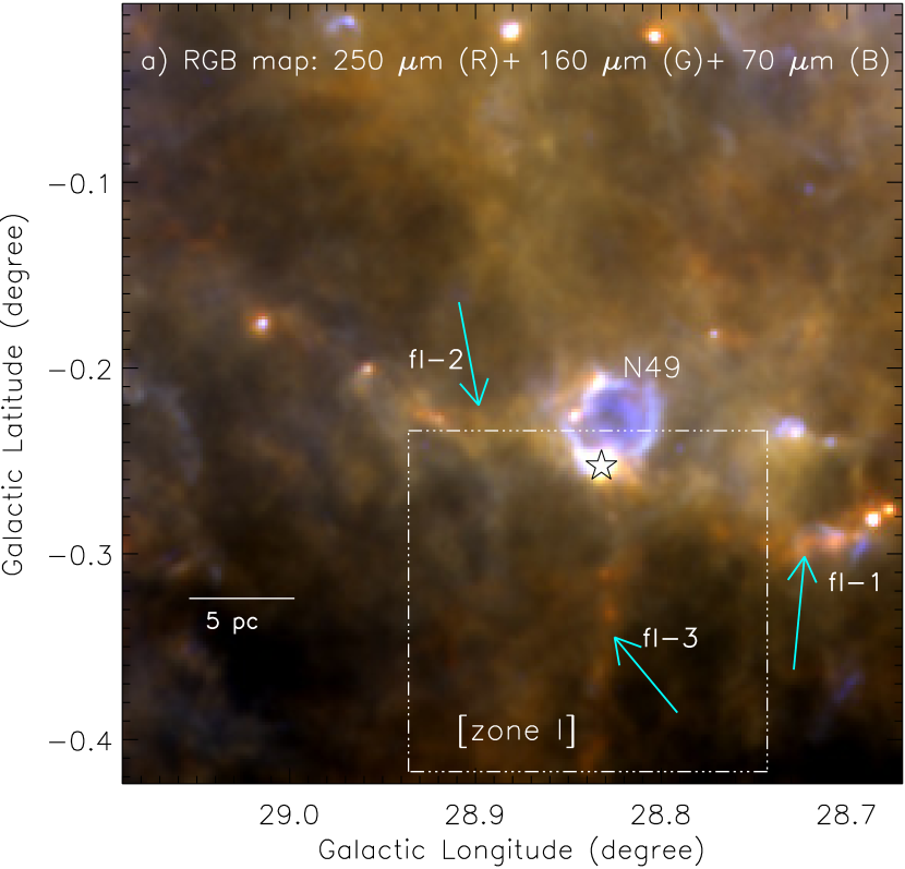
Figure 1.— a) Large-scale view of the MIR bubble N49 (size of the selected field $\sim$0$\arcdeg$.42 $\times$ 0$\arcdeg$.42 ($\sim$37.2 pc $\times$ 37.2 pc); central coordinates: $l$ = 28$\arcdeg$.844; $b$ = $-$0$\arcdeg$.220). a) A three color-composite map (Herschel 250 $\mu$m (red), 160 $\mu$m (green), and 70 $\mu$m (blue) images in log scale). The MIR bubble N49 is prominently seen in the composite map. Three arrows highlight the embedded filaments. A position of the Class II 6.7 GHz methanol maser (from Szymczak et al., 2012) is shown by a star, which is traced in a velocity range of 79.4 to 92.7 km s^-1. A scale bar corresponding to 5 pc is shown in the bottom left corner. b) The GRS ¹³CO (1-0) spectrum in the direction of a small field (i.e. zone I; see highlighted box in Figure 1a). The spectrum reveals three velocity components in the direction of zone I and is obtained by averaging the area.

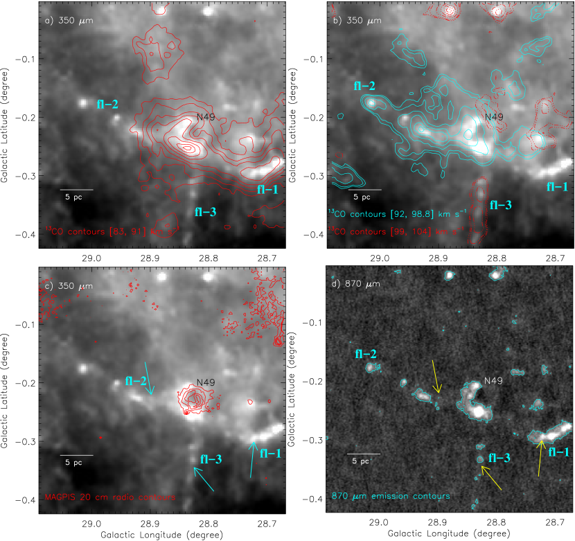
Figure 2.— a) Overlay of the molecular ¹³CO gas on the Herschel 350 $\mu$m image. The ¹³CO integrated velocity range is from 83 to 91 km s^-1. The ¹³CO contours are 40.847 K km s^-1 $\times$ (0.12, 0.2, 0.3, 0.4, 0.55, 0.7, 0.85, 0.95). b) The ¹³CO emissions are superimposed on the Herschel 350 $\mu$m image. The cyan and red contours represent ¹³CO integrated over two different velocity ranges highlighted in the image. The CO contours (in cyan) are 38.357 K km s^-1 $\times$ (0.35, 0.4, 0.55, 0.7, 0.85, 0.95), while the levels of red contours are 21.468 K km s^-1 $\times$ (0.35, 0.4, 0.55, 0.7, 0.85, 0.95). c) Overlay of the MAGPIS 20 cm contours on the Herschel 350 $\mu$m image. The contours (in red) are shown with levels of 0.0243 Jy/beam $\times$ (0.06, 0.1, 0.14, 0.18). d) Overlay of the ATLASGAL 870 $\mu$m contour on the ATLASGAL 870 $\mu$m image. A contour (in cyan) is shown with a level of 0.163 Jy/beam. In each panel, a scale bar corresponding to 5 pc is shown in the bottom left corner. In the panels c and d, three arrows highlight the embedded filamentary features.

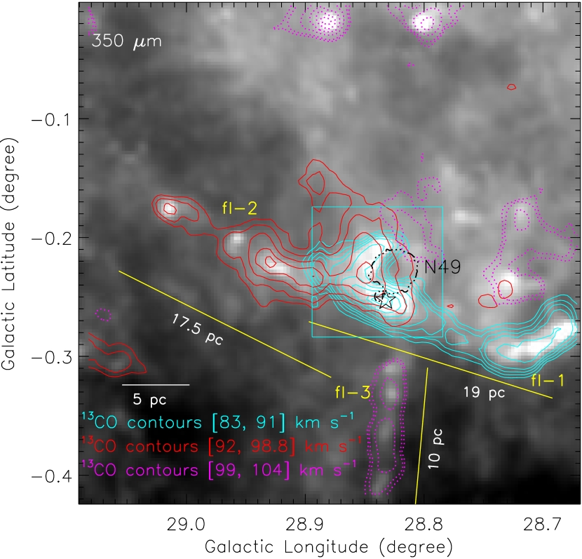
Figure 3.— Overlay of the molecular clouds linked with the filamentary features on the Herschel 350 $\mu$m image. The ¹³CO emissions integrated over three different velocity ranges are presented and the velocity ranges are also given in the figure (also see Figures 2a and 2b). The ¹³CO contours (in red) are 38.357 K km s^-1 $\times$ (0.45, 0.55, 0.7, 0.85, 0.95), while the levels of cyan contours are 40.847 K km s^-1 $\times$ (0.35, 0.4, 0.45, 0.5, 0.6, 0.7, 0.8, 0.9, 0.95). The ¹³CO contours (in magenta) are similar to those shown in Figures 2b. A broken contour at 20 cm (in black) represents the location of the bubble N49, and the contour level is 0.0024 Jy/beam. A position of the Class II 6.7 GHz methanol maser (from Szymczak et al., 2012) is shown by a black star. The solid box (in cyan) encompasses the area shown in Figures 4a-l and 5a. A scale bar corresponding to 5 pc is shown in the bottom left corner.

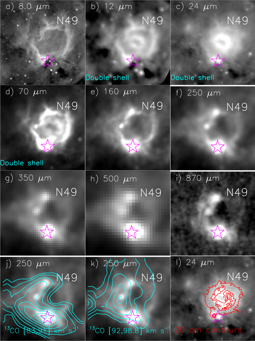
Figure 4.— A multi-wavelength view of the bubble N49. The images are shown at different wavelengths, which are highlighted in the panels. In the panels “j” and “k”, the ¹³CO emissions are superimposed on the Herschel 250 $\mu$m image. The ¹³CO integrated velocity ranges are also shown in these panels. In the panel “j”, the ¹³CO contours are 40.847 K km s^-1 $\times$ (0.35, 0.4, 0.5, 0.6, 0.7, 0.8, 0.9, 0.98). In the panel “k”, the ¹³CO contours are 38.357 K km s^-1 $\times$ (0.6, 0.7, 0.8, 0.9, 0.98). In the panel “l”, the MAGPIS 20 cm emission is superimposed on the Spitzer 24 $\mu$m image. The MAGPIS contours (in red) are shown with levels of 0.0018, 0.0035, 0.0045, and 0.005 Jy/beam. In each panel, a position of the Class II 6.7 GHz methanol maser is shown by a star.

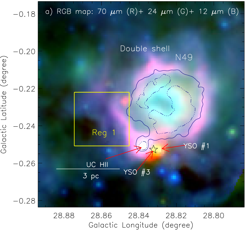
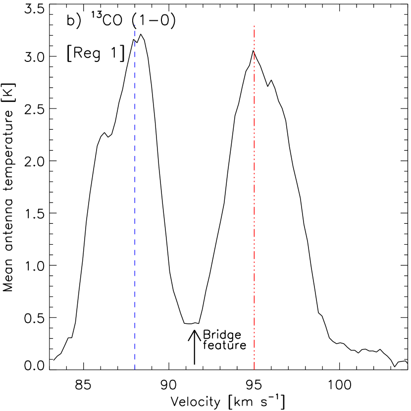
Figure 5.— Three-color composite image (red, Herschel 70 $\mu$m; green, Spitzer 24 $\mu$m; blue,WISE 12 $\mu$m; in log scale) of the bubble N49, which clearly traces a double shell structure. The contours at 20 cm (in navy) are also overlaid on the composite image, and the contour levels are 0.0024 and 0.00353 Jy/beam. A position of the Class II 6.7 GHz methanol maser is shown by a star. Previously three known sources (i.e. ”UC HII”, “YSO #1”, and “YSO #3”) are marked and highlighted by arrows in the figure (also see Figure 1 in Zavagno et al., 2010). A scale bar corresponding to 3 pc is shown in the bottom left corner. b) The GRS ¹³CO (1-0) spectrum in the direction of a small field (i.e. Reg 1; see highlighted box in Figure 5a). The spectrum is obtained by averaging the area, Reg 1. Two velocity peaks are highlighted by broken lines. An almost flattened profile is found between two velocity peaks (i.e. a bridge feature).

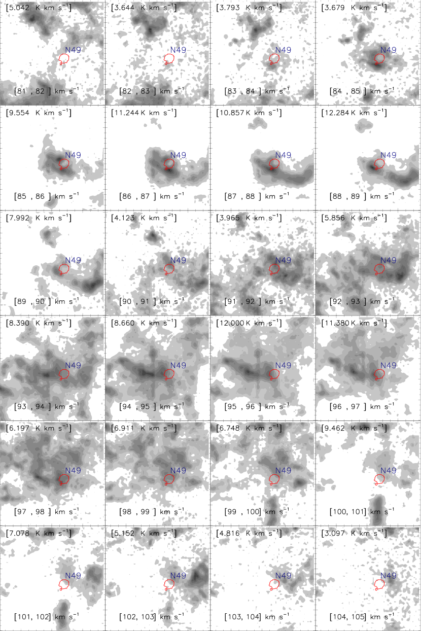
Figure 6.— The ¹³CO(J =1$-$0) velocity channel contour maps. The molecular emission is integrated over a velocity interval, which is given in each panel (in km s^-1). The contour levels are 10, 20, 30, 40, 55, 70, 80, 90, and 99% of the peak value (in K km s^-1), which is also given in each panel. In each panel, a contour at 20 cm (in red) represents the location of the bubble N49, and the contour level is 0.0024 Jy/beam.

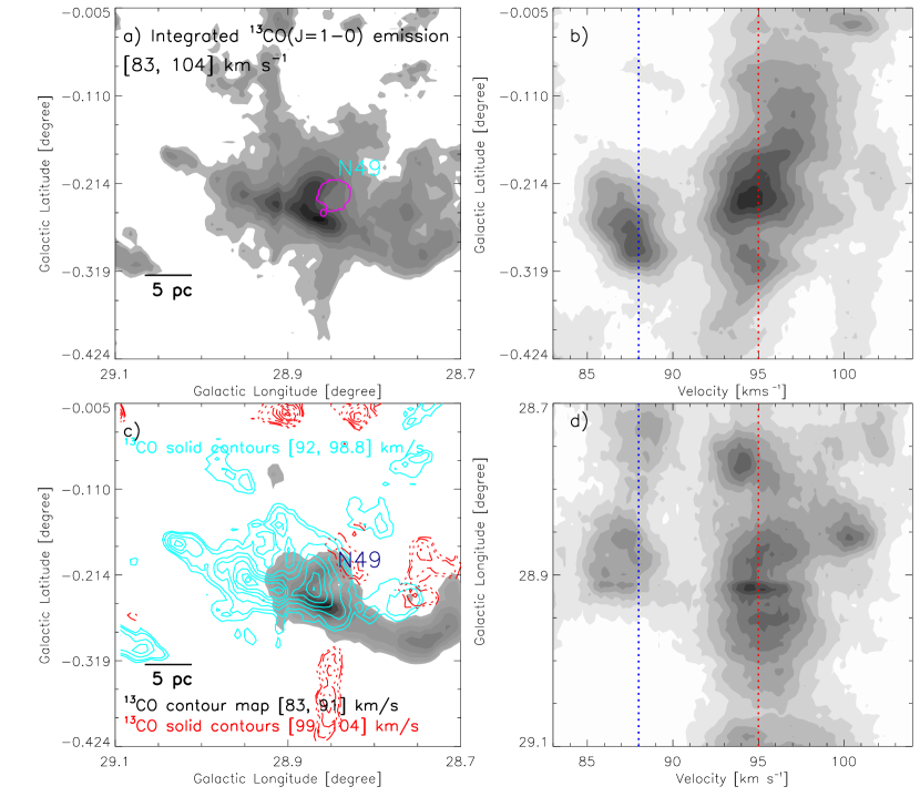
Figure 7.— a) Integrated intensity map of ¹³CO (J = 1-0) from 83 to 104 km s^-1. The contour levels are 25, 30, 40, 50, 60, 70, 80, 90, and 95% of the peak value (i.e. 71.408 K km s^-1). A contour at 20 cm (in magenta) represents the location of the bubble N49, and the contour level is 0.0024 Jy/beam. b) Latitude-velocity map of ¹³CO. The ¹³CO emission is integrated over the longitude from 28$\arcdeg$.67 to 29$\arcdeg$.09. c) The ¹³CO emissions integrated over three different velocity ranges are presented, and the velocity ranges are also given in the panel (also see Figures 2a and 2b). d) Longitude-velocity map of ¹³CO. The ¹³CO emission is integrated over the latitude from $-$0$\arcdeg$.424 to $-$0$\arcdeg$.005. In both the left panels (i.e. Figures 7a and 7c), the scale bar corresponding to 5 pc is shown in the bottom left corner. Two dotted lines are also shown in both the right panels (i.e. Figures 7b and 7d), and are similar to those shown in Figure 5b.

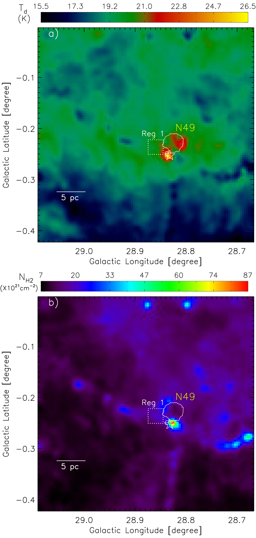
Figure 8.— a) Herschel temperature map. b) Herschel column density ($N(\mathrm{H}_{2})$) map. One can also compute the extinction value with $A_{V}=1.07\times 10^{-21}~{}N(\mathrm{H}_{2})$ (Bohlin et al., 1978). A position of the Class II 6.7 GHz methanol maser is shown by a star in each panel. In both the panels, a small dotted square indicates the area, Reg1, which is similar to those shown in Figure 5a. In each panel, a contour at 20 cm (in pink) represents the location of the bubble N49, and the contour level is 0.0024 Jy/beam. In both the panels, the scale bar corresponding to 5 pc is shown in the bottom left corner.

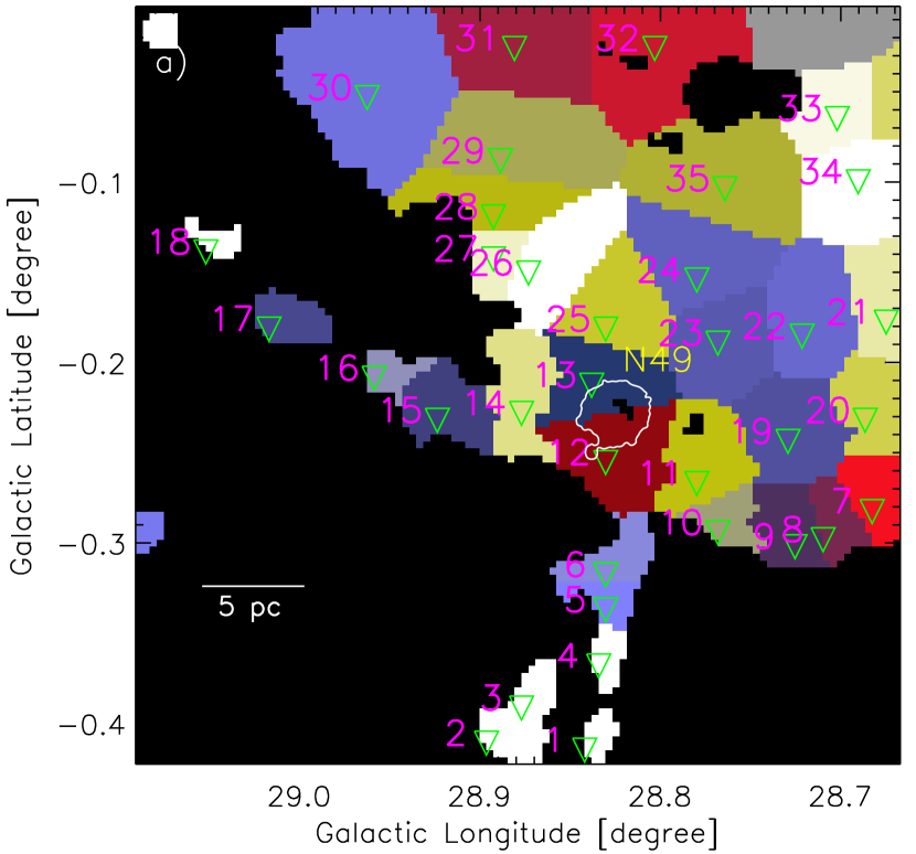
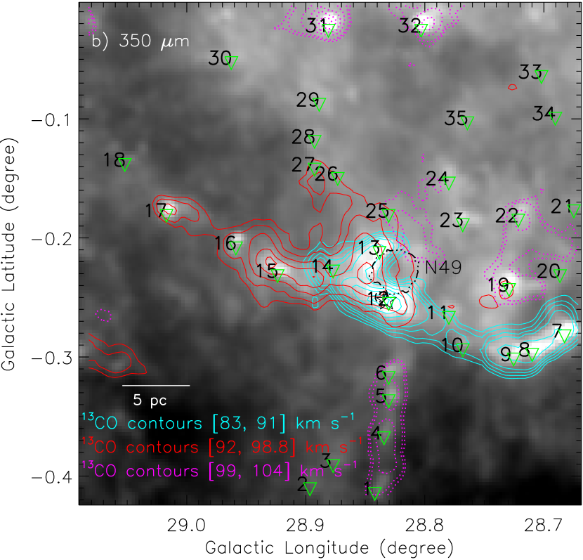
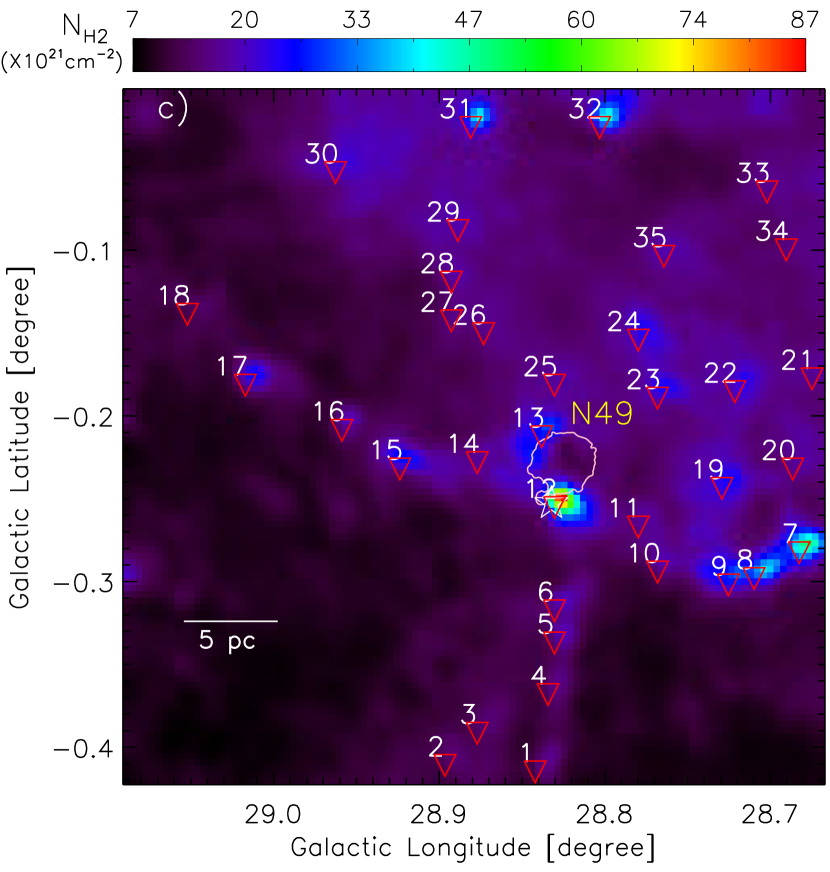
Figure 9.— The selected Herschel clumps in our selected target field. a) The clumps are shown by upside down triangles, and the boundary of each Herschel clump is also highlighted along with its corresponding clump ID (see Table 1). A contour at 20 cm (in white) represents the location of the bubble N49, and the contour level is 0.0024 Jy/beam. b) Overlay of the positions of the clumps (i.e. upside down triangles) along their IDs and the molecular clouds on the Herschel image at 350 $\mu$m. The background map and the molecular clouds are similar to those shown in Figure 3. c) The positions of the clumps (i.e. upside down triangles) along their IDs are also overlaid on the Herschel column density map. The background map is similar to those shown in Figure 8b. In each panel, the scale bar corresponding to 5 pc is shown in the bottom left corner.

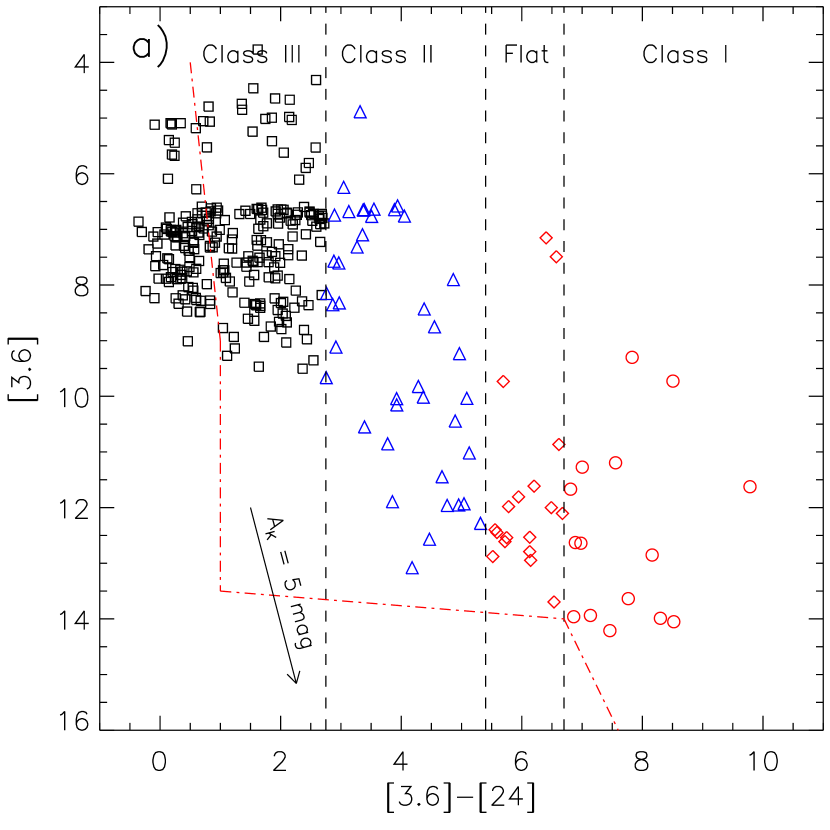
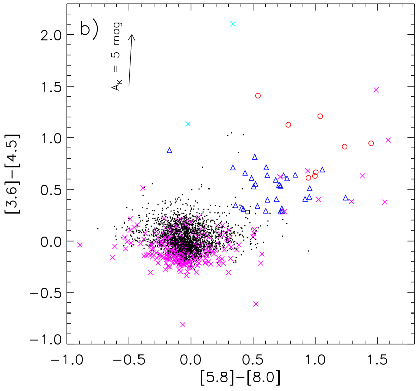
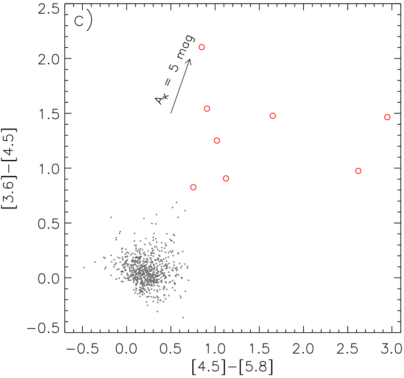
Figure 10.— Selection of YSOs in our selected field around the MIR bubble N49 (see Figure 1a). a) Color-magnitude plot ([3.6] $-$ [24] vs [3.6]) of sources. The plot enables to identify YSOs belonging to different evolutionary stages (see dashed lines). The boundary of YSOs against contaminated candidates (galaxies and disk-less stars) is shown by dotted-dashed lines (in red) (see Rebull et al. (2011) for more details). Flat-spectrum and Class III sources are represented by “$\Diamond$” and “$\Box$” symbols, respectively. b) Color-color plot ([3.6]$-$[4.5] vs. [5.8]$-$[8.0]) of sources. The PAH-emitting galaxies and the PAH-emission-contaminated apertures are marked by “*” and “$\times$” symbols, respectively (see the text). A Class III source is represented by a black square in the plot. c) Color-color plot ([3.6]$-$[4.5] vs. [4.5]$-$[5.8]) of sources. In the panels “a”, “b”, and “c”, we show Class I (circles) and Class II (open triangles) YSOs. In the first three panels, an extinction vector is shown and is obtained using the average extinction laws from Flaherty et al. (2007). In the panels “b” and “c”, the dot symbols show the stars with only photospheric emissions. Due to large numbers of stars with photospheric emissions, only some of these stars are randomly marked in the panels “b” and “c”.

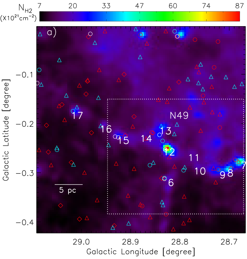
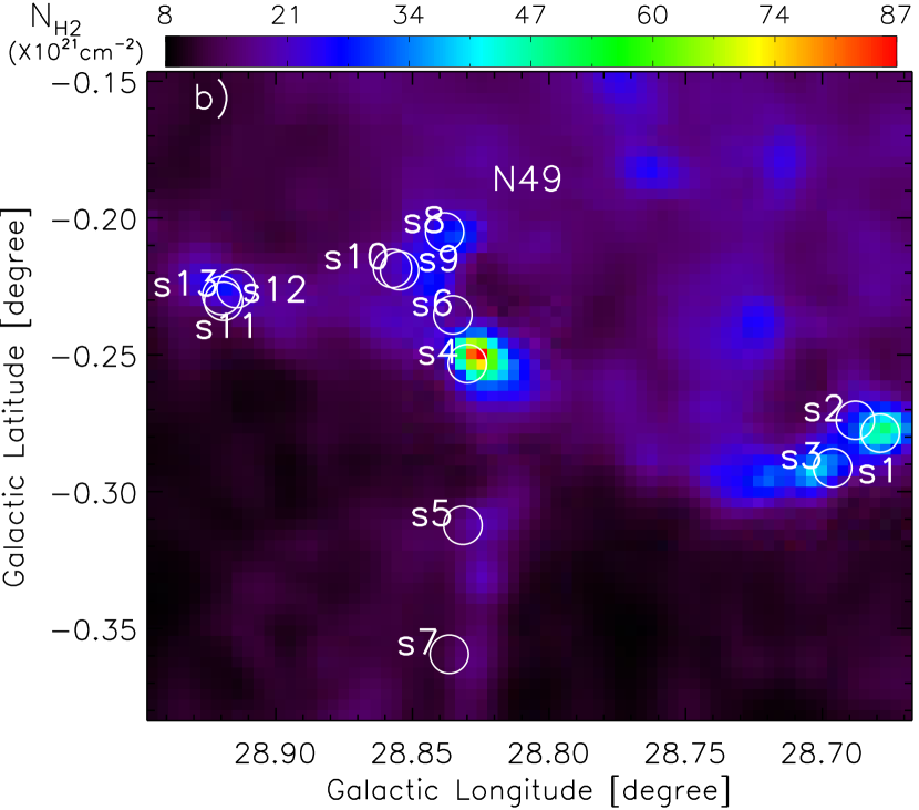
Figure 11.— a) Spatial distribution of YSOs in our selected field around the MIR bubble N49. The YSOs (Class I (circles), Flat-spectrum (diamond), and Class II (triangles)) are overlaid on the Herschel column density map. The background map is similar to the one shown in Figure 8b. The YSOs (in red) are selected using the color-magnitude ([3.6] $-$ [24] vs [3.6]) scheme (see Figure 10a), while the YSOs (in cyan) are identified using the color-color ([3.6]$-$[4.5] vs. [5.8]$-$[8.0]) scheme (see Figure 10b). The Class I YSOs selected via the color-color ([3.6]$-$[4.5] vs. [4.5]$-$[5.8]) scheme are highlighted by white circles (see Figure 10c). The Herschel clump IDs 6–17 are also marked in the figure (also see Figure 9b). A broken box (in white) encompasses the area shown in Figure 11b. b) The positions of some selected YSOs are marked along their IDs on the Herschel column density map (see white circles and also Table 2). These YSOs are found toward the edges of the bubble and the filamentary features. The physical properties of these YSOs are listed in Table 2.

Table 1Physical parameters of the Herschel clumps (see Figures 9a and 9b). Column 1 gives the IDs assigned to the clump. Table also lists Galactic coordinates (l, b), deconvolved effective radius (R_clump), and clump mass (M_clump). The clumps (nos. 12, 13, and 14) are highlighted by daggers, and are found in the intersection zone of two filamentary molecular clouds (see Figure 9b).

ID	l	b	Rclump	Mclump
	[degree]	[degree]	(pc)	($M_{\odot}$)
1	28.842	-0.415	1.0	1076
2	28.897	-0.411	1.4	1821
3	28.877	-0.392	1.4	1954
4	28.834	-0.368	1.2	1397
5	28.830	-0.337	1.3	1836
6	28.830	-0.318	1.7	3161
7	28.683	-0.283	1.8	5317
8	28.710	-0.298	1.6	3761
9	28.725	-0.302	2.0	5569
10	28.768	-0.294	1.5	2638
11	28.780	-0.267	2.4	6177
12†	28.830	-0.255	2.7	11538
13†	28.838	-0.213	2.5	8480
14†	28.877	-0.228	2.4	5800
15	28.924	-0.232	2.1	5483
16	28.959	-0.209	1.2	1599
17	29.017	-0.182	1.6	2876
18	29.052	-0.139	1.0	948
19	28.729	-0.244	2.7	9451
20	28.687	-0.232	2.1	5114
21	28.675	-0.178	2.1	4741
22	28.722	-0.185	2.8	9734
23	28.768	-0.189	2.7	8807
24	28.780	-0.154	2.9	10093
25	28.830	-0.182	2.6	7418
26	28.873	-0.150	2.7	7671
27	28.893	-0.143	1.5	2464
28	28.893	-0.119	2.3	5761
29	28.889	-0.088	3.4	13112
30	28.963	-0.053	4.2	20970
31	28.881	-0.026	3.2	12381
32	28.803	-0.026	3.3	12885
33	28.702	-0.065	2.2	5134
34	28.690	-0.100	2.5	6592
35	28.764	-0.104	3.5	12804

Table 2Physical parameters derived from SED fitting of some selected YSOs (see Figure 11b), which are taken from Dirienzo et al. (2012) (see Table 4 in their paper). Column 1 gives the IDs assigned to the YSO. Table also lists YSO designation, $\chi^{2}_{best}$ per data points, stellar mass (M_∗), and stellar luminosity (L_∗) (see Dirienzo et al. (2012) for more details). The YSOs distributed toward the edges of the bubble, filaments fl-1, fl-2, and fl-3 are highlighted with labels “bub”, fl1, fl2, and fl3, respectively (see Figure 11b).

ID	YSO	($\chi^{2}_{best}$/n${}_{data})$	M∗	L∗
	(designation (lb))		($M_{\odot}$)	($L_{\odot}$)
s1fl1	028.6788-00.2786	0.05	3.8$\pm$1.1	102.3$\pm$102.6
s2fl1	028.6879-00.2739	0.31	3.6$\pm$1.3	102.0$\pm$102.1
s3fl1	028.6962-00.2913	0.47	5.0$\pm$1.6	102.9$\pm$103.1
s4bub	028.8299-00.2532	0.39	6.2$\pm$2.0	103.1$\pm$103.2
s5fl3	028.8315-00.3123	0.49	2.4$\pm$1.5	102.0$\pm$102.4
s6bub	028.8352-00.2354	0.04	4.1$\pm$1.4	102.5$\pm$102.8
s7fl3	028.8365-00.3594	0.17	4.0$\pm$1.3	102.5$\pm$102.8
s8bub	028.8382-00.2051	0.15	3.5$\pm$1.0	102.2$\pm$102.5
s9bub	028.8547-00.2192	1.80	2.8$\pm$1.8	102.3$\pm$102.5
s10bub	028.8573-00.2184	0.54	1.6$\pm$1.3	101.8$\pm$102.2
s11fl2	028.9145-00.2258	1.60	3.1$\pm$0.8	101.8$\pm$102.0
s12fl2	028.9191-00.2304	0.10	1.1$\pm$1.0	101.6$\pm$102.0
s13fl2	028.9198-00.2283	1.39	5.0$\pm$1.7	102.9$\pm$103.1

References

- Anathpindika (2010) Anathpindika, S. V. 2010, MNRAS, 405, 1431
- Anderson & Bania (2009) Anderson, L. D., & Bania, T. M. 2009, ApJ, 690, 706
- Benjamin et al. (2003) Benjamin, R. A., Churchwell, E., Babler, B. L., et al. 2003, PASP, 115, 953
- Bisbas et al. (2017) Bisbas, T. G., Tanaka, K. E. I., Tan, J. C., Wu, B., & Nakamura, F. 2017, arXiv:1706.07006
- Bohlin et al. (1978) Bohlin, R. C., Savage, B. D., & Drake, J. F. 1978, ApJ, 224, 13233
- Carey et al. (2005) Carey, S. J., Noriega-Crespo, A., Price, S. D., et al. 2005, BAAS, 37, 1252
- Churchwell et al. (2006) Churchwell, E., Povich, M. S., Allen, D., et al. 2006, ApJ, 649, 759
- Cyganowski et al. (2009) Cyganowski, C. J., Brogan, C. L., Hunter, T. R., Churchwell, E. 2009, ApJ, 702, 1615
- de Graauw et al. (2010) de Graauw, T., Helmich, F. P., Phillips, T. G., et al. 2010, A&A, 518, L4
- Deharveng et al. (2010) Deharveng, L., Schuller, F., Anderson, L. D., et al. 2010, A&A, 523, 6
- Dewangan & Anandarao (2011) Dewangan, L. K., & Anandarao, B. G. 2011, MNRAS, 414, 1526
- Dewangan et al. (2015) Dewangan, L. K., Luna, A., Ojha, D. K., et al. 2015, ApJ, 811, 79
- Dewangan (2017a) Dewangan, L. K. 2017a, ApJ, 837, 44
- Dewangan & Ojha (2017b) Dewangan, L. K., & Ojha, D. K. 2017b, in ApJ press, arXiv:1709.06251
- Dirienzo et al. (2012) Dirienzo, W. J., Indebetouw, R., Brogan, C., et al. 2012, AJ, 144, 173
- Evans et al. (2009) Evans, N. J., II, Dunham, M. M., Jrgensen, J. K., et al. 2009, ApJS, 181, 321
- Everett & Churchwell (2010) Everett, J. E., & Churchwell, E. 2010, ApJ, 713, 592
- Flaherty et al. (2007) Flaherty, K. M., Pipher, J. L., Megeath, S. T., et al. 2007, ApJ, 663, 1069
- Fukui et al. (2014) Fukui, Y., Ohama, A., Hanaoka, N., et al. 2014, ApJ, 780, 36
- Fukui et al. (2016) Fukui, Y., Torii, K., Ohama, A., et al. 2016, ApJ, 820, 26
- Furukawa et al. (2009) Furukawa, N., Dawson, J. R., Ohama, A., et al. 2009, ApJL, 696, L115
- Getman et al. (2007) Getman, K. V., Feigelson, E. D., Garmire,G., Broos, P., & Wang, J. 2007, ApJ, 654, 316
- Griffin et al. (2010) Griffin, M. J., Abergel, A., Abreu, A, et al. 2010, A&A, 518L, 3
- Guieu et al. (2010) Guieu, S., Rebull, L. M., Stauffer, J. R., et al. 2010, ApJ, 720, 46
- Gutermuth et al. (2009) Gutermuth, R. A., Megeath, S. T., Myers, P. C., et al. 2009, ApJS, 184, 18
- Gutermuth & Heyer (2015) Gutermuth, R. A., & Heyer, M. 2015, AJ, 149, 64
- Habe & Ohta (1992) Habe, A., & Ohta, K. 1992, PASJ, 44, 203
- Hartmann et al. (2005) Hartmann, L., Megeath, S. T., Allen, L., et al. 2005, ApJ, 629, 881
- Haworth et al. (2015a) Haworth, T. J., Tasker, E. J., Fukui, Y., et al. 2015a, MNRAS, 450, 10
- Haworth et al. (2015b) Haworth, T. J., Shima, K., Tasker, E. J., et al. 2015b, MNRAS, 454, 1634
- Helfand et al. (2006) Helfand, D. J., Becker, R. H., White, R. L., Fallon, A., & Tuttle, S. 2006, AJ, 131, 2525
- Hildebrand (1983) Hildebrand, R. H. 1983, Quarterly Journal of the RAS, 24, 267
- Inoue & Fukui (2013) Inoue, T., & Fukui, Y. 2013, ApJL, 774, 31
- Jackson et al. (2006) Jackson, J. M., Rathborne, J. M., Shah, R. Y., et al. 2006, ApJS, 163, 145
- Kauffmann et al. (2008) Kauffmann, J., Bertoldi, F., Bourke, T. L., Evans, II, N. J., & Lee, C. W. 2008, ApJ, 487, 993
- Lada et al. (2006) Lada, C. J., Muench, A. A., Luhman, K. L., et al. 2006, AJ, 131, 1574
- Liu et al. (2017) Liu, HL, Figueira, M., Zavagno, A., et al. 2017, A&A, 602, 95
- Mallick et al. (2015) Mallick, K. K., Ojha, D. K., Tamura, M., et al. 2015, MNRAS, 447, 2307
- Ohama et al. (2010) Ohama, A., Dawson, J. R., Furukawa, N., et al. 2010, ApJ, 709, 975
- Ott (2010) Ott, S. 2010, in Astronomical Society of the Pacic Conference Series, Vol. 434, Astronomical Data Analysis Software and Systems XIX, ed. Y. Mizumoto, K.-I. Morita, & M. Ohishi, 139
- Pilbratt et al. (2010) Pilbratt, G. L., Riedinger, J. R., Passvogel, T., et al. 2010, A&A, 518, L1
- Poglitsch et al. (2010) Poglitsch, A., Waelkens, C., Geis, N., et al. 2010, A&A, 518L, 2
- Rebull et al. (2011) Rebull, L. M., Guieu, S., Stauffer, J. R., et al. 2011, ApJS, 193, 25
- Schuller et al. (2009) Schuller, F., Menten, K. M., Contreras, Y., et al. 2009, A&A, 504, 415
- Szymczak et al. (2012) Szymczak, M., Wolak, P., Bartkiewicz, A., & Borkowski, K. M. 2012, AN, 333, 634
- Takahira et al. (2014) Takahira, K., Tasker, E. J., & Habe, A. 2014, ApJ, 792, 63
- Tan et al. (2014) Tan, J. C., Beltrán, M. T., Caselli, P., et al. 2014, in Protostars and Planets VI, ed. H. Beuther et al. (Tucson, AZ: Univ. Arizona Press), 149
- Torii et al. (2015) Torii, K., Hasegawa, K., Hattori, Y., et al. 2015, ApJ, 806, 7
- Torii et al. (2017) Torii, K., Hattori, Y., Hasegawa, K., et al. 2017, ApJ, 835, 142
- Urquhart et al. (2013) Urquhart, J. S., Moore, T. J. T., Schuller, F., et al. 2013, MNRAS, 431, 1752
- Walsh et al. (1998) Walsh, A. J., Burton, M. G., Hyland, A. R., & Robinson, G. 1998, MNRAS, 301, 640
- Watson et al. (2008) Watson, C., Povich, M. S., Churchwell, E. B., et al. 2008, ApJ, 681, 1341
- Williams et al. (1994) Williams, J. P., de Geus, E. J., & Blitz, L. 1994, ApJ, 428, 693
- Wright et al. (2010) Wright, E. L., Eisenhardt, P. R. M., Mainzer, A. K., et al. 2010, AJ, 140, 1868
- Zavagno et al. (2010) Zavagno, A., Anderson, L. D., Russeil, D., et al. 2010, A&A, 518, 101
- Zinnecker & Yorke (2007) Zinnecker, H., & Yorke, H. W. 2007, ARA&A, 45, 481