Abstract

Transmission of a normally incident plane wave through a metasurface with bicontrollable subwavelength scattering elements was simulated using a commercial software. Some pixels comprising the $\sf{H}$-shaped scattering elements were made of a magnetostatically controllable material whereas the remaining pixels were made of a thermally controllable material, the metasurface designed to operate in the terahertz spectral regime. The co-polarized transmission coefficients were found to exhibit stopbands that shift when either a magnetostatic field is applied or the temperature is increased or both. Depending on spectral location of the stopband, either the magnetostatic field gives coarse control and temperature gives fine control or vice versa. The level of magnetostatic control depends on the magnetostatic-field configuration.

1 Introduction

A frequency-selective-surface (FSS) is a planar periodic array of identical scattering elements [1, 2]. The elements are electrically thin in the direction normal to the surface. Each element is either infinitely long in one direction on the surface or has finite dimensions in any direction on the surface. Typically, FSSs are used as bandpass and bandstop filters as well as to redirect a plane wave in a nonspecular direction.

If the lattice parameters (and, therefore, the linear dimensions of the scattering elements) of a 2D FSS are sufficiently small fractions of the free-space wavelength $\lambda_{\scriptscriptstyle 0}$, and the wave vector of the incident plane wave is directed not very obliquely, the transmitted field contains a plane wave propagating in the specular direction along with a multitude of evanescent plane waves that are nonspecular. The 2D FSS is then more commonly referred to as a metasurface these days [3, 4, 5, 6].

Metasurfaces are useful in bandstop filters [7, 8], absorbers [9], and polarimeters [10]. Metasurfaces that generate local phase changes can be used to control the wavefront [13, 12]. Application to holography is another area of research interest [11]. Thus, metasurfaces are attractive for molding electromagnetic-wave propagation in a variety of ways.

This attraction is quite pronounced in the terahertz (THz) regime. Within this spectral regime, significant benefits can be realized for power electronics [14], imaging [15], spectroscopy [16], sensing [17], cancer detection [18], and so on. THz imaging has immense potential for security technology, as it can extract the spectroscopic fingerprints of a wide range of chemicals used in explosives and biological weapons [19].

The concept of multicontrollable metasurfaces has recently been put forth, with inspiration from biological examples of multicontrollability [20]. Each subwavelength scattering element in a multicontrollable metasurface is a set of non-overlapping pixels. All pixels in a specific subset are made of a specific material, and the scattering element is made of at least two different materials. The electromagnetic constitutive parameters of each of these materials in the chosen spectral regime may be controlled by the variation of a specific environmental parameter such as temperature, voltage, and a magnetostatic field. Thus, the overall electromagnetic response characteristics of a multicontrollable metasurface can be dynamically controlled using one or more modalities.

In order to establish the feasibility of multicontrollable metasurfaces, in this paper we present theoretical results on the THz transmission characteristics of a bicontrollable metasurface whose scattering elements comprise magnetostatically controllable pixels made of InAs [7, 6] and thermally controllable pixels made of CdTe [21]. The chosen metasurface and the simulation method are described in Sec. 2 Numerical results of transmission simulations are presented in Sec. 3 to establish the desired bicontrollability. Conclusions follow under Sec. 4.

An $\exp\left(-i\omega t\right)$ dependence on time $t$ is implicit, with $\omega=2\pi\nu$ denoting the angular frequency, $\nu$ the linear frequency, and $i=\sqrt{-1}$. The free-space wavenumber and the intrinsic impedance of free space are denoted by $k_{\scriptscriptstyle 0}=\omega\sqrt{\varepsilon_{\scriptscriptstyle 0}\mu_{\scriptscriptstyle 0}}=2\pi/\lambda_{\scriptscriptstyle 0}$ and $\eta_{\scriptscriptstyle 0}=\sqrt{\mu_{\scriptscriptstyle 0}/\varepsilon_{\scriptscriptstyle 0}}$, respectively, with $\varepsilon_{\scriptscriptstyle 0}$ and $\mu_{\scriptscriptstyle 0}$ being the permittivity and permeability of free space. Vectors are in boldface; dyadics are underlined twice; and the three Cartesian unit vectors are identified as ${\bf u}_{x}$, ${\bf u}_{y}$, and ${\bf u}_{z}$.

2 Materials and Method

The unit cell of the chosen bicontrollable metasurface is a rectangular parallelepiped of dimensions $a\times{a}\times(t+b)$ aligned with the $x$, $y$, and $z$ axes, as shown in Fig. 1. The substrate occupies the region $z\in(-t-b,-t)$ and is made of an isotropic material with relative permittivity $\varepsilon_{d}$. The active region of the unit cell is a rectangular parallelepiped of dimensions $(2w+l)\times{h}\times{t}$ aligned with the $x$, $y$, and $z$ axes, with $(2w+l)\leq{a}$, $h\leq{a}$, and $t\ll{a}$. The active region is made of

• two $w\times{h}\times{t}$ sections and one $l\times{w}\times{t}$ section, together forming an $\sf{H}$ and all three comprising pixels made of a magnetostatically controllable material, and

• two $l\times{(1/2)(h-w)}\times{t}$ sections comprising pixels made of a thermally controllable material.

For calculations, we chose InAs as the magnetostatically controllable material [6, 7] and CdTe as the thermally controllable material [21].

(a)

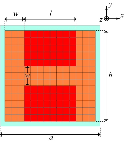
(b)

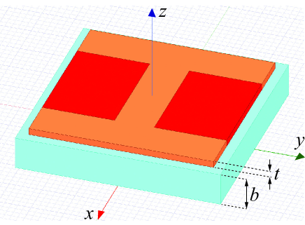
Figure 1: (Color online) (a) Top and (b) isometric views of the unit cell of the chosen bicontrollable metasurface comprising magnetostatically controllable (orange) and thermally controllable (red) pixels deposited on an inert substrate (blue). Various linear dimensions as well as the Cartesian axes are also shown.

InAs is an isotropic dielectric material in the absence of an external magnetostatic field and its relative permittivity can be appropriately represented by the Drude model [22]. When it is subjected to a magnetostatic field ${\bf B}_{\scriptscriptstyle 0}$, InAs functions as a gyroelectric material [7, 6]. Its relative permittivity dyadic then depends on the magnitude $B_{\scriptscriptstyle 0}=|{\bf B}_{\scriptscriptstyle 0}|$ and the direction ${\bf B}_{\scriptscriptstyle 0}/B_{\scriptscriptstyle 0}$ of ${\bf B}_{\scriptscriptstyle 0}$. The following three configurations are distinctive:

• Faraday configuration (${\bf B}_{\scriptscriptstyle 0}\parallel{\bf u}_{z}$), with the relative permittivity dyadic

  $$\underline{\underline{\varepsilon}}_{InAs}^{F}=\varepsilon_{\perp}\left({\bf u}_{x}{\bf u}_{x}+{\bf u}_{y}{\bf u}_{y}\right)+\varepsilon_{\parallel}{\bf u}_{z}{\bf u}_{z}+\varepsilon_{\times}\left({\bf u}_{x}{\bf u}_{y}-{\bf u}_{y}{\bf u}_{x}\right)\,;$$ (1)

• Voigt-X configuration (${\bf B}_{\scriptscriptstyle 0}\parallel{\bf u}_{x}$), with the relative permittivity dyadic

  $$\underline{\underline{\varepsilon}}_{InAs}^{VX}=\varepsilon_{\perp}\left({\bf u}_{y}{\bf u}_{y}+{\bf u}_{z}{\bf u}_{z}\right)+\varepsilon_{\parallel}{\bf u}_{x}{\bf u}_{x}+\varepsilon_{\times}\left({\bf u}_{y}{\bf u}_{z}-{\bf u}_{z}{\bf u}_{y}\right)\,;$$ (2)

  and

• Voigt-Y configuration (${\bf B}_{\scriptscriptstyle 0}\parallel{\bf u}_{y}$), with the relative permittivity dyadic

  $$\underline{\underline{\varepsilon}}_{InAs}^{VY}=\varepsilon_{\perp}\left({\bf u}_{x}{\bf u}_{x}+{\bf u}_{z}{\bf u}_{z}\right)+\varepsilon_{\parallel}{\bf u}_{y}{\bf u}_{y}+\varepsilon_{\times}\left({\bf u}_{z}{\bf u}_{x}-{\bf u}_{x}{\bf u}_{z}\right)\,.$$ (3)

In

$$\left.\begin{array}[]{l}\varepsilon_{\perp}=\varepsilon_{\infty}-\displaystyle\frac{\bar{\omega}_{p}^{2}\left(1+i\bar{\gamma}\right)}{\left(1+i\bar{\gamma}\right)^{2}-\bar{\omega}_{c}^{2}}\\[8.0pt] \varepsilon_{\parallel}=\varepsilon_{\infty}-\displaystyle\frac{\bar{\omega}_{p}^{2}}{\left(1+i\bar{\gamma}\right)}\,,\\[8.0pt] \varepsilon_{\times}=i\displaystyle\frac{\bar{\omega_{c}}\bar{\omega}_{p}^{2}}{\left(1+i\bar{\gamma}\right)^{2}-\bar{\omega}_{c}^{2}}\end{array}\right\}\,,$$ (4)

$\varepsilon_{\infty}=16.3$ is the value assumed by the relative permittivity in the limit $\omega\rightarrow\infty$; $\bar{\omega}_{p}=\omega_{p}/\omega$ is the normalized plasma frequency with $\omega_{p}=\sqrt{N_{e}q_{e}^{2}/\varepsilon_{\scriptscriptstyle 0}m^{\ast}}$ as the plasma frequency, $N_{e}=1.04\times 10^{23}$ m^-3 as the free-career density, $m^{\ast}=4\times 10^{-3}m_{e}$ as the effective carrier mass, $m_{e}=9.11\times 10^{-31}$ kg as the electron mass, and $q_{e}=1.6\times 10^{-19}$ C as the elementary charge; $\bar{\gamma}=\gamma/\omega$ is the normalized damping constant with $\gamma=15\pi\times 10^{11}$ rad s^-1 as the damping constant; $\bar{\omega}_{c}=\omega_{c}/\omega$ is the normalized cyclotron frequency with $\omega_{c}=q_{e}B_{\scriptscriptstyle 0}/m^{\ast}$ as the cyclotron frequency that provides the dependence of the relative permittivity dyadic on the magnitude $B_{\scriptscriptstyle 0}$ of the magnetostatic field. In this paper, we provide results for $B_{\scriptscriptstyle 0}=0$ T and $B_{\scriptscriptstyle 0}=1$ T to simulate an on-off switching scenario.

CdTe is an isotropic dielectric material whose relative permittivity changes as a function of the temperature in the THz regime. However, CdTe is also an electro-optic material so that we invoked the Pockels effect by the application of an electrostatic field  [23, 24]. When CdTe is subjected to a dc electric field ${\bf E}_{dc}=E_{dc}{\bf u}_{z}$, its acts like an orthorhombic dielectric material with relative permittivity dyadic

$$\underline{\underline{\varepsilon}}_{CdTe}=\varepsilon_{\alpha}\left({\bf u}_{x}{\bf u}_{x}+{\bf u}_{y}{\bf u}_{y}\right)+\varepsilon_{\beta}\left({\bf u}_{x}{\bf u}_{y}+{\bf u}_{y}{\bf u}_{x}\right)+\varepsilon_{\gamma}{\bf u}_{z}{\bf u}_{z}$$ (5)

where

$$\left.\begin{array}[]{l}\varepsilon_{\alpha}=\displaystyle\frac{\varepsilon_{\gamma}}{1-r_{\gamma}^{2}E_{dc}^{2}\varepsilon_{\gamma}^{2}}\\[8.0pt] \varepsilon_{\beta}=-\displaystyle\frac{r_{\gamma}E_{dc}\varepsilon_{\gamma}^{2}}{1-r_{\gamma}^{2}E_{dc}^{2}\varepsilon_{\gamma}^{2}}\end{array}\right\}\,,$$ (6)

$r_{\gamma}=6.8\times 10^{-12}$ m V^-1 is the electro-optic coefficient, and $\varepsilon_{\gamma}$ is the relative permittivity in the absence of dc electric field. Due to temperature dependence, we have [21]

$$\varepsilon_{\gamma}=\varepsilon_{hf}+\displaystyle\frac{\left(\varepsilon_{dc}-\varepsilon_{hf}\right)\omega_{T}^{2}}{\omega_{T}^{2}-\omega^{2}-i\gamma_{T}\omega}$$ (7)

where $\varepsilon_{hf}=6.8$ is the high-frequency relative permittivity, $\omega_{T}$ is the resonance angular frequency, $\gamma_{T}$ is the damping constant, and $\varepsilon_{dc}$ is the static relative permittivity. The latter three parameters can be expressed as quadratic functions of the absolute temperature $T$ as

$$Y=A+B\left(\displaystyle\frac{T}{T_{ph}}\right)+C\left(\displaystyle\frac{T}{T_{ph}}\right)^{2}\,,\qquad Y\in\left\{\omega_{T},\gamma_{T},\varepsilon_{dc}\right\}\,,$$ (8)

where $T_{ph}=207$ K is the characteristic phonon temperature of CdTe. The coefficients $A$, $B$, and $C$ are given in Table 1 for the application of Eq. (8) to $\omega_{T}$, $\gamma_{T}$, and $\varepsilon_{dc}$. In order to calculate all numerical results presented here, we set $E_{dc}=10^{6}$ V m^-1 which is far below the dielectric-breakdown limit $10^{7}$ V m^-1 of CdTe.

Table 1: Coefficients of quadratic thermal dependences in the Eq. (8) for $\omega_{T}$, $\gamma_{T}$, and $\varepsilon_{dc}$ of CdTe.

Parameter	$A$	$B$	$C$	Units
$\omega_{T}\times 10^{-12}$	$27.401$	$-0.1872$	$-0.2187$	rad s-1
$\gamma_{T}/\omega_{T}$	$0.0116$	$0.0314$	$0.0119$
$\varepsilon_{dc}$	$9.808$	$0.1719$	$0.1414$

An arbitrarily polarized plane wave was considered to impinge normally on the face $z=0$ of the chosen metasurface. Hence, the incident electric field phasor can be written as

$${\bf E}_{inc}=\left(E_{0x}{\bf u}_{x}+E_{0y}{\bf u}_{y}\right)\exp\left(-ik_{\scriptscriptstyle 0}z\right),\quad z>0.$$ (9)

For all calculations, we set either

• $E_{0x}=1$ V m^-1 and $E_{0y}=0$ for $x$-polarized incidence or

• $E_{0x}=0$ and $E_{0y}=1$ V m^-1 for $y$-polarized incidence.

The dimensions of the unit cell were chosen so that all nonspecular components of the transmitted field are evanescent. Therefore, far from the face $z=-t-b$ as $z\to-\infty$, the transmitted electric field phasor can be written as

$${\bf E}_{tr}=\left[\left(\tau_{xx}E_{0x}+\tau_{xy}E_{0y}\right){\bf u}_{x}+\left(\tau_{yy}E_{0y}+\tau_{yx}E_{0x}\right){\bf u}_{y}\right]$$

$$\qquad\times\exp\left(-ik_{\scriptscriptstyle 0}z\right),\quad z\to-\infty,$$ (10)

where $\tau_{xx}$ and $\tau_{yy}$ are the co-polarized specular transmission coefficients whereas $\tau_{xy}$ and $\tau_{yx}$ are the cross-polarized specular transmission coefficients.

The response characteristics of the chosen metasurface to the normally incident plane wave were obtained using the 3D electromagnetic simulator ANSYS® [25]. The simulator considered only the unit cell with periodicity imposed with respect to both $x$ and $y$, Floquet theory [26, 27] being invoked to represent the $x$- and $y$-variations of the electric and magnetic field phasors.

The actual structure simulated is constituted by the unit cell and two $a\times{a}\times{d}$ vacuous regions, one above and the other below the unit cell along the $z$ axis, with $d\simeq\lambda_{\scriptscriptstyle 0}/4$. The following four-step iterative procedure involving an adaptive mesh was used to obtain convergent results:

• A mesh is generated with tetrahedrons of certain dimensions.

• The electromagnetic boundary-value problem is solved to determine the scattering matrix of the analyzed structure.

• Another mesh with smaller tetrahedrons is generated and step (ii) is repeated.

• A test is performed on the non-zero elements of the scattering matrixes obtained in steps (ii) and (iii). If no element changes by more than $0.1\%$ in magnitude, the procedure is stopped. If not, the second mesh is designated as the first mesh a new iteration and steps (ii)–(iv) are repeated.

The iterative procedure was started with an initial mesh comprising tetrahedrons having a maximum dimension $0.2\lambda_{\scriptscriptstyle 0}$ and the tetrahedron dimensions were reduced by $20\%$ every iteration. Convergence was reached within 12 iterations.

3 Results and Discussions

For all data reported here, we fixed $a=18.36$ $\upmu$m, $b=2.5$ $\upmu$m, $t=0.5$ $\upmu$m, $w=3.6$ $\upmu$m, $l=9.6$ $\upmu$m, $h=16.8$ $\upmu$m, and $\varepsilon_{d}=2.1$. Calculations were made for $f=\omega/2\pi\in\left[0.5,5.5\right]$ THz with $T\in\left\{233,373\right\}$ K and $B_{\scriptscriptstyle 0}\in\left\{0,1\right\}$ T. For all three configurations of the magnetostatic field, $\tau_{xy}$ and $\tau_{yx}$ turned out to be negligibly small. Hence, we present spectrums of only $|\tau_{xx}|$ and $|\tau_{yy}|$ in this section.

3.1 Stopbands of $\tau_{xx}$

3.1.1 First stopband

The spectrums of $\left|\tau_{xx}\right|$ for all three distinctive configurations of the magnetostatic field are presented in Fig. 2 for $B_{\scriptscriptstyle 0}\in\left\{0,1\right\}$ T and $T\in\left\{233,373\right\}$ K. A prominent stopband (transmission less than $-7$ dB) exists between 1.3 and 1.7 THz in all spectrums. Let the baseline environmental parameters be specified as $B_{\scriptscriptstyle 0}=0$ and $T=233$ K (black curves in Fig. 2), for which the center frequency $\nu_{\rm c}$ of the stopband is $1.678$ THz. Obviously, since $B_{\scriptscriptstyle 0}=0$, this value of $\nu_{\rm c}$ is the same for all three magnetostatic-field configurations: Faraday [Fig. 2(a)], Voigt-X [Fig. 2(b)], and Voigt-Y [Fig. 2(c)]. Increasing the temperature to the high value ($T=373$ K) results in a small redshift of the spectrums (red curves), with $\nu_{\rm c}$ decreasing to $1.674$ THz. The percentage relative shift $\Delta\nu_{\rm c}/\nu_{\rm c}=-0.24\%$ of the center frequency ($\Delta\nu_{\rm c}=-4$ GHz) must be due to the CdTe pixels because the effect of temperature on the relative permittivity of InAs was assumed to be small enough to be ignored, and magnetostatic effects on the relative permittivity of CdTe were ignored similarly.

(a)

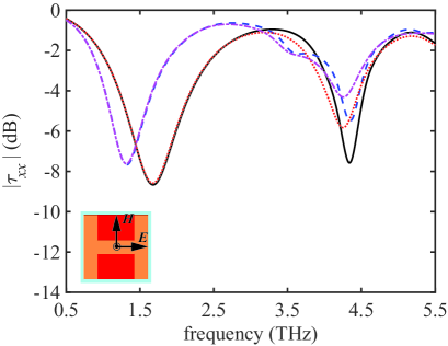
(b)

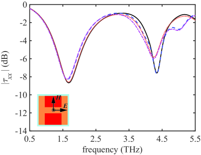
(c)

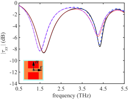
Figure 2: (Color online) Spectrums of $|\tau_{xx}|$ for (a) Faraday, (b) Voigt-X, and (c) Voigt-Y configurations. The solid black curves are for $B_{0}=0$ T and $T=233$ K, the dotted red curves for $B_{0}=0$ T and $T=373$ K, the dashed blue curves for $B_{0}=1$ T and $T=233$ K, and the dashed-dotted magenta curves for $B_{0}=1$ T and $T=373$ K. The insets show the polarization state of the incident plane wave.

Increasing the magnitude of the magnetostatic field from $0$ to $1$ T instead of increasing the temperature produces a larger redshift (blue curves) with respect to the baseline (black curves). In the Faraday configuration, $\nu_{\rm c}$ redshifts from $1.678$ THz to $1.321$ THz when $B_{\scriptscriptstyle 0}$ changes from $0$ to $1$ T at a fixed temperature of $233$ K, the shift $\Delta\nu_{\rm c}=-357$ GHz, and a percentage relative shift of $\Delta\nu_{\rm c}/\nu_{\rm c}=-21.28\%$, of the center frequency being huge. The redshift of $\nu_{\rm c}$ is less strong in the Voigt-Y configuration: from $1.678$ THz to $1.507$ THz resulting in $\Delta\nu_{\rm c}/\nu_{\rm c}=-10.19\%$. The redshift is even weaker for the Voigt-X configuration: from $1.678$ THz to $1.637$ THz resulting in $\Delta\nu_{\rm c}/\nu_{\rm c}=-2.44\%$. All three of these shifts must be due to the InAs pixels because the CdTe pixels cannot be affected by the magnetostatic field.

Switching on the $1$-T magnetostatic field and increasing the temperature from $233$ K to $373$ K simultaneously invokes the magnetostatic controllability of the InAs pixels and the thermal controllability of the CdTe pixels in a cooperative fashion. The center frequency $\nu_{\rm c}$ of the stopband shifts by $-362$ GHz, $-45$ GHz, and $-177$ GHz to $1.316$ THz, $1.633$ THz, and $1.501$ THz, corresponding to a percentage relative shift $\Delta\nu_{\rm c}/\nu_{\rm c}=-21.57\%$, $-2.68\%$, and $-10.55\%$ for the Faraday, Voigt-X, and Voigt-Y configuration, respectively.

The central frequencies of the stopband of $\tau_{xx}$ in the range 1.3–1.7-THz range for all magnetostatic-field configurations and chosen values of the magnetostatic field and temperature are provided in Table 2. The data indicate (i) that the magnetostatic field gives coarse control whereas temperature gives fine control, and (ii) that $B_{\scriptscriptstyle 0}$ and $T$ act cooperatively.

Table 2: Center frequencies (THz) of the first stopband (between 1.3 and 1.7 THz) of $\left|\tau_{xx}\right|$ for $B_{0}=\left\{0,1\right\}$ T and $T=\left\{233,373\right\}$ K for the Faraday, Voigt-X, and Voigt-Y configurations.

Magnetostatic	$B_{\scriptscriptstyle 0}=0$ T	$B_{\scriptscriptstyle 0}=0$ T	$B_{\scriptscriptstyle 0}=1$ T	$B_{\scriptscriptstyle 0}=1$ T
configuration	$T=233$ K	$T=373$ K	$T=233$ K	$T=373$ K
Faraday	1.678	1.674	1.321	1.316
Voigt-X	1.678	1.674	1.637	1.633
Voigt-Y	1.678	1.674	1.507	1.501

The metasurface response depends on the magnetostatic-field configuration because of the asymmetry of the $\sf{H}$ shape. Thus, rotation about the $z$ axis by 90 deg changes the resonator shape, allowing a distinction between the responses for the Voigt-X and Voigt-Y configurations. Rotation about the $z$ axis, however, can not affect the response for the Faraday configuration.

3.1.2 Second stopband

The spectrums of $\left|\tau_{xx}\right|$ presented in Fig. 2 exhibit a second stopband in the 4.2–4.4-THz range. When $B_{\scriptscriptstyle 0}=0$ and $T=233$ K, the center frequency $\nu_{\rm c}$ of the second stopband is $4.340$ THz, as identified in Table 3. Raising the temperature to $373$ K without turning on the magnetostatic field results in a shift of $-87$ GHz, the percentage relative bandwidth shift $\Delta\nu_{\rm c}/\nu_{\rm c}=-2.00\%$ being about 22 times larger than of the first stopband. Thus, the thermal-control modality due to the CdTe pixels is more effective in the higher-frequency part of the $[0.5,5.5]$-THz range.

Table 3: Center frequencies (THz) of the second stopband (between 4.2 and 4.4 THz) of $\left|\tau_{xx}\right|$ for $B_{0}=\left\{0,1\right\}$ T and $T=\left\{233,373\right\}$ K for the Faraday, Voigt-X, and Voigt-Y configurations.

Magnetostatic	$B_{\scriptscriptstyle 0}=0$ T	$B_{\scriptscriptstyle 0}=0$ T	$B_{\scriptscriptstyle 0}=1$ T	$B_{\scriptscriptstyle 0}=1$ T
configuration	$T=233$ K	$T=373$ K	$T=233$ K	$T=373$ K
Faraday	4.340	4.253	4.349	4.258
Voigt-X	4.340	4.253	4.340	4.250
Voigt-Y	4.340	4.253	4.320	4.229

The effect of the InAs pixels by themselves is different on the second stopband from that on the first stopband. In the Faraday configuration, $\nu_{\rm c}$ blueshifts from $4.340$ THz to $4.349$ THz when $B_{\scriptscriptstyle 0}$ changes from $0$ to $1$ T at a fixed temperature of $233$ K, so that the the percentage relative percentage shift $\Delta\nu_{\rm c}/\nu_{\rm c}=0.21\%$. Concurrently, no shift at all is evident for the Voigt-X configuration whereas the shift is $-20$ GHz (i.e., $\Delta\nu_{\rm c}/\nu_{\rm c}={0.46}\%$) for the Voigt-Y configuration. In contrast, the first stopband redshifted by much larger margins for all three magnetostatic-field configurations.

By switching on the $1$-T magnetostatic field and increasing the temperature from $233$ K to $373$ K simultaneously, the center frequency $\nu_{\rm c}$ of the second stopband shifts by $-82$ GHz, $-90$ GHz, and $-11$ GHz to $4.258$ THz, $4.250$ THz, and $4.229$ THz corresponding to a percentage relative shift $\Delta\nu_{\rm c}/\nu_{\rm c}=-1.89\%$, $-2.07\%$, and $-2.56\%$ for the Faraday, Voigt-X, and Voigt-Y configuration, respectively. All three shifts are redshifts, just the same as for the first stopband. However, the data in Table 3 indicate (i) that the magnetostatic field gives fine control whereas temperature gives coarse control, and (ii) that $B_{\scriptscriptstyle 0}$ and $T$ act cooperatively for the Faraday and the Voigt-X configurations but not for the Voigt-Y configuration.

Table 4: Spatial profiles of the electric and magnetic fields on the top surface of the unit cell at the center frequency $\nu_{\rm c}$ of the first stopband of $\tau_{xx}$, when the magnetostatic field is in the Faraday configuration. The normalization factors are ${E_{inc}}=+\sqrt{|{E_{0x}}|^{2}+|{E_{0y}}|^{2}}$ and ${H_{inc}=E_{inc}}/\eta_{\scriptscriptstyle 0}$.

In order to examine how the switching the magnetostatic field on/off as well as the raising/lowering the temperature affects the transmission spectrums, we calculated the field distributions at the center frequencies of the first stopbands of $\left|\tau_{xx}\right|$ when the magnetostatic field is in the Faraday configuration. Spatial profiles of the electric and magnetic fields at the center frequencies of the first stopband are shown in Table 4 for combinations of $B_{0}\in\left\{0,1\right\}$ T and $T\in\left\{233,373\right\}$ K. Clearly, a change in temperature affects the spatial profile of the magnetic field significantly, particularly in the CdTe region close to the central section of the $\sf H$ (made of InAs), but not much the spatial profile of the electric field. Likewise, a change in the magnetostatic field affects the spatial profile of the electric field significantly, particularly in the central section as well as at the extremities of both legs of the $\sf H$, but the spatial profile of the electric field is insignificantly affected. In passing, let us note that at corners and edges, the electric field can be more than hundred times larger than the amplitude of the incident electric field and the magnetic field can be more ten times larger than the amplitude of the incident magnetic field.

3.2 Stopbands of $\tau_{yy}$

3.2.1 First stopband

Figure 3 is analogous to Fig. 2, except that the spectrums of $\left|\tau_{yy}\right|$ instead of $\left|\tau_{xx}\right|$ are plotted. Similarly to what has been observed for $\left|\tau_{xx}\right|$, $\left|\tau_{yy}\right|$ exhibits a prominent stopband (transmission less than $-11$ dB) between $2.5$ and $3.1$ THz. For the baseline condition specified as $B_{\scriptscriptstyle 0}=0$ and $T=233$ K (black curves in Fig. 3), the center frequency $\nu_{\rm c}$ of the stopband is $3.055$ THz for all three magnetostatic-field configurations: Faraday [Fig. 3(a)], Voigt-X [Fig. 3(b)], and Voigt-Y [Fig. 3(c)]. Increasing the temperature from $233$ K to $373$ K results in the redshift of $\nu_{\rm c}$ from $3.055$ to $3.032$ THz due to the CdTe pixels. The percentage relative shift being $\Delta\nu_{\rm c}/\nu_{\rm c}=-0.75\%$, the shift $\Delta\nu_{\rm c}=-23$ GHz is about six times larger in magnitude than the one for $\tau_{xx}$.

(a)

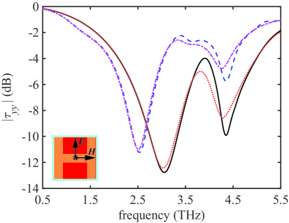
(b)

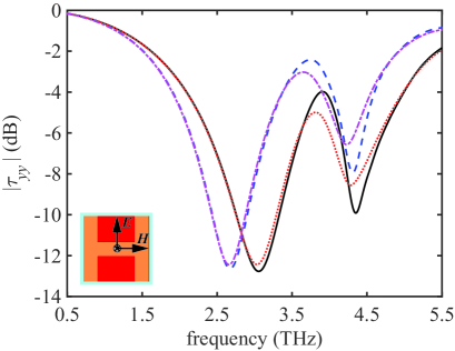
(c)

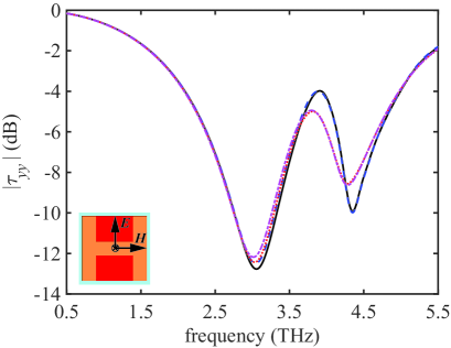
Figure 3: (Color online) Same as Fig. 2, but the spectrums of $|\tau_{yy}|$ are shown.

Unlike what was found for $\tau_{xx}$, switching on the $1$-T magnetostatic field while keeping the temperature fixed at $233$ K produces a significantly larger redshift (blue curves) for $\tau_{yy}$ with respect to the baseline for the Faraday and Voigt-X configurations but a significantly smaller redshift for the Voigt-Y configuration, as becomes clear from comparing Tables 2 and 5. The shift is $-524$ GHz, $-381$, and $-11$ GHz, corresponding to the percentage relative shift $\Delta\nu_{\rm c}/\nu_{\rm c}=-17.15\%$, $-12.47\%$, and $-0.36\%$, respectively, for the Faraday, Voigt-X, and Voigt-Y configuration. These shifts are due to the InAs pixels.

Table 5: Center frequencies (THz) of the first stopband (between $2.5$ and $3.1$ THz) of $\left|\tau_{yy}\right|$ for $B_{0}=\left\{0,1\right\}$ T and $T=\left\{233,373\right\}$ K for the Faraday, Voigt-X, and Voigt-Y configurations.

Magnetostatic	$B_{\scriptscriptstyle 0}=0$ T	$B_{\scriptscriptstyle 0}=0$ T	$B_{\scriptscriptstyle 0}=1$ T	$B_{\scriptscriptstyle 0}=1$ T
configuration	$T=233$ K	$T=373$ K	$T=233$ K	$T=373$ K
Faraday	3.055	3.032	2.531	2.510
Voigt-X	3.055	3.032	2.674	2.659
Voigt-Y	3.055	3.032	3.044	3.015

By switching on the $1$-T magnetostatic field and increasing the temperature from $233$ K to $373$ K simultaneously, even larger redshifts become evident in the spectrums of $\left|\tau_{yy}\right|$ (magenta curves) in Fig. 3. The central frequency $\nu_{\rm c}$ of the stopband shifts to $2.510$ THz, $2.659$ THz, and $3.015$ THz, for the Faraday, Voigt-X, and Voigt-Y configuration, respectively, the shift being $-545$ GHz, $-396$ GHz, and $-40$ GHz and the percentage relative bandwidth shift is $\Delta\nu_{\rm c}/\nu_{\rm c}=-17.84\%$, $-12.96\%$, and $-1.31\%$, correspondingly. Thus, both $B_{\scriptscriptstyle 0}$ and $T$ act cooperatively for $\tau_{yy}$, just as for $\tau_{xx}$.

3.2.2 Second stopband

The spectrums of $\left|\tau_{yy}\right|$ presented in Fig. 3 exhibit a second stopband in the $4.2$–$4.4$ THz frequency range. For all three distinctive configurations of the magnetostatic field, unlike what was observed for the first stopband in Sec. 3.3.2.1, fine control comes from the magnetostatic field and coarse control from the temperature, as may also be deduced from the data presented in Table 6.

Table 6: Center frequencies (THz) of the second stopband (between $4.2$ and $4.4$ THz) of $\left|\tau_{yy}\right|$ for $B_{0}=\left\{0,1\right\}$ T and $T=\left\{233,373\right\}$ K for the Faraday, Voigt-X, and Voigt-Y configurations.

Magnetostatic	$B_{\scriptscriptstyle 0}=0$ T	$B_{\scriptscriptstyle 0}=0$ T	$B_{\scriptscriptstyle 0}=1$ T	$B_{\scriptscriptstyle 0}=1$ T
configuration	$T=233$ K	$T=373$ K	$T=233$ K	$T=373$ K
Faraday	4.352	4.282	4.352	4.259
Voigt-X	4.352	4.282	4.312	4.229
Voigt-Y	4.352	4.282	4.351	4.285

Table 7: Spatial profiles of the electric and magnetic fields on the top surface of the unit cell at the center frequency $\nu_{\rm c}$ of the first stopband of $\tau_{yy}$, when the magnetostatic field is in the Voigt-X configuration. The normalization factors are ${E_{inc}}=+\sqrt{|{E_{0x}}|^{2}+|{E_{0y}}|^{2}}$ and ${H_{inc}=E_{inc}}/\eta_{\scriptscriptstyle 0}$.

Indeed, for the baseline condition specified as $B_{\scriptscriptstyle 0}=0$ and $T=233$ K (black curves in Fig. 3), the center frequency $\nu_{\rm c}$ of the stopband is $4.352$ THz for all three magnetostatic-field configurations. Increasing the temperature from $233$ K to $373$ K while keeping the magnetostatic field null valued results in the redshift of $\nu_{\rm c}$ from $4.352$ to $4.282$ THz, i.e., $\Delta\nu_{\rm c}/\nu_{\rm c}=-1.61\%$ and $\Delta\nu_{\rm c}=-70$ GHz. This shift is comparable to the shift observed for the second stopband in the spectrum of $\tau_{xx}$ in Sec. 3.3.1.2. Switching on the $1$-T magnetostatic field instead of increasing the temperature from $233$ K produces a shift of $0$ GHz, $-40$, and $-1$ GHz, with a percentage relative shift $\Delta\nu_{\rm c}/\nu_{\rm c}=0\%$, $-0.92\%$, and $-0.02\%$, correspondingly. respectively, for the Faraday, Voigt-X, and Voigt-Y configuration. Clearly, the thermal control modality is much more effective than the magnetostatic control modality.

Switching on the $1$-T magnetostatic field and increasing the temperature from $233$ K to $373$ K simultaneously makes the center frequency of the second stopband shift by $-93$ GHz, $-123$, and $-67$ GHz to $4.259$ THz, $4.229$ THz, and $4.285$ THz giving a percentage relative shift $\Delta\nu_{\rm c}/\nu_{\rm c}=-2.14\%$, $-2.83\%$, and $-1.54\%$. for the Faraday, Voigt-X, and Voigt-Y configuration, respectively. We conclude that $B_{\scriptscriptstyle 0}$ and $T$ act cooperatively.

Spatial profiles of the electric and magnetic fields at the center frequencies of the first stopband are shown in Table 7 for combinations of $B_{0}\in\left\{0,1\right\}$ T and $T\in\left\{233,373\right\}$ K for the Voigt-X configurations. Clearly, a change in the magnetostatic field affects the spatial profile of the magnetic field significantly, particularly in the central section and both legs of the $\sf H$ made of InAs, but the spatial profile of the electric field is not affected much. Likewise, a change in temperature field affects the spatial profile of the electric field significantly, particularly in the CdTe regions close to the legs of the $\sf H$, but not significantly the spatial profile of the magnetic field.

4 Concluding remarks

We have theoretically substantiated the concept of multicontrollability for metasurfaces by employing two differently controllable materials in the $\sf{H}$-shaped subwavelength scattering elements of a specific metasurface. The transmission spectrums of the chosen metasurface exhibit prominent stopbands in the THz regime. These stopbands shift when either thermally controllable pixels in the scattering elements are influenced by increasing the temperature or the magnetostatically controllable pixels in the scattering elements are influenced by turning on a magnetostatic field. Depending on the spectral location of the stopband, either the magnetostatic field gives coarse control and temperature gives fine control or vice versa. The level of magnetostatic control depends on the magnetostatic-field configuration. The largest shifts emerge when both control modalities are simultaneously deployed.

Other control modalities—such as electrical, optical, piezoelectric, and magnetostrictive [28]—can be invoked by using pixels made of diverse materials [20]. Numerous geometries are possible for the subwavelength scattering elements [30, 29]. We plan to report our further work on multicontrollable metasurfaces in appropriate forums.

Acknowledgment. AL thanks the Charles Godfrey Binder Endowment at Penn State for ongoing support of his research.

References

- [1] T.-K. Wu, Frequency Selective Surfaces (Wiley, 1995).
- [2] B. A. Munk, Frequency Selective Surfaces: Theory and Design (Wiley, 2000).
- [3] C. L. Holloway, E. R. Kuester, and D. R. Novotny, “Waveguides composed of metafilms/metasurfaces: The two-dimensional equivalent of metamaterials,” IEEE Antennas Wireless Propag. Lett. 8, 525–529 (2009).
- [4] M. Veysi, C. Guclu, O. Boyraz, and F. Capolino, “Thin anisotropic metasurfaces for simultaneous light focusing and polarization manipulation,” J. Opt. Soc. Am. B 32, 318–323 (2015).
- [5] J. Chen and H. Mosallaei, “Truly achromatic optical metasurfaces: a filter circuit theory-based design,” J. Opt. Soc. Am. B 32, 2115–2121 (2015).
- [6] A. E. Serebryannikov, A. Lakhtakia, and E. Ozbay, “Single and cascaded, magnetically controllable metasurfaces as terahertz filters,” J. Opt. Soc. Am. B 33, 834–841 (2016).
- [7] J. Han, A. Lakhtakia, and C.-W. Qiu, “Terahertz metamaterials with semiconductor split-ring resonators for magnetostatic tunability,” Opt. Express 16, 14390–14396 (2008).
- [8] W. Min, H. Sun, Q. Zhang, H. Ding, W. Shen, and X. Sun, “A novel dual-band terahertz metamaterial modulator,” J. Optics (Bristol) 18, 065103 (2016).
- [9] X. Liu, K. Fan, I. V. Shadrivov, and W. J. Padilla, “Experimental realization of a terahertz all-dielectric metasurface absorber,” Opt. Express 25, 191–201 (2017).
- [10] J. P. B. Mueller, K. Leosson, and F. Capasso, “Ultracompact metasurface in-line polarimeter,” Optica 3, 42–47 (2016).
- [11] E. Hack and P. Zolliker, “Terahertz holography for imaging amplitude and phase objects,” Opt. Express 22, 16080–16086 (2014).
- [12] L. Huang, X. Chen, H. Mühlenbernd, G. Li, B. Bai, Q. Tan, G. Jin, T. Zentgraf, and S. Zhang, “Dispersionless phase discontinuities for controlling light propagation,” Nano Lett. 12, 5750–5755 (2012).
- [13] S. L. Jia, X. Wan, P. Su, Y. J. Zhao, and T. J. Cui, “Broadband metasurface for independent control of reflected amplitude and phase,” AIP Adv. 6, 045024 (2016).
- [14] R. Sinha, M. Karabiyik, A. Ahmadivand, C. Al-Amin, P. K. Vabbina, M. Shur, and P. Nezih, “Tunable, room temperature CMOS-compatible THz emitters based on nonlinear mixing in microdisk resonators,” J. Infrared Millim. Terahertz Waves 37, 230–242 (2016).
- [15] J. Y. Suen and W. J. Padilla, “Superiority of terahertz over infrared transmission through bandages and burn wound ointments,” Appl. Phys. Lett. 108, 233701 (2016).
- [16] J. Qin, L. Xie, and Y. Ying, “A high-sensitivity terahertz spectroscopy technology for tetracycline hydrochloride detection using metamaterials,” Food Chem. 211, 300–305 (2016).
- [17] S. R. J. Bhatt, P. Bhatt, P. Deshmukh, B. R. Sangala, M. N. Satyanarayan, G. Umesh, and S. S. Prabhu, “Resonant terahertz InSb waveguide device for sensing polymers,” J. Infrared Millim. Terahertz Waves 37, 795–804 (2016).
- [18] S. K. Yngvesson, A. Karellas, S. Glick, A. Khan, P. R. Siqueira, P. A. Kelly, and B. St. Peter, “Breast cancer margin detection with a single frequency terahertz imaging system,” Proc. SPIE 9706, 970603 (2016).
- [19] R. E. Miles, X.-C. Zhang, H. Eisele, and A. Krotkus (Eds.), Terahertz Frequency Detection and Identification of Materials and Objects (Springer, 2007).
- [20] A. Lakhtakia, D. E. Wolfe, M. W. Horn, J. Mazurowski, A. Burger, and P. P. Banerjee, “Bioinspired multicontrollable metasurfaces and metamaterials for terahertz applications,” Proc. SPIE 10162, 101620V (2017).
- [21] M. Schall, M. Walther, and P. U. Jepsen, “Fundamental and second-order phonon processes in CdTe and ZnTe,” Phys. Rev. B 64, 094301 (2001).
- [22] M. G. Blaber, M. D. Arnold, and M. J. Ford, “A review of the optical properties of alloys and intermetallics for plasmonics,” J. Phys.: Condens. Matter 22, 143201 (2010).
- [23] C. A. Valagiannopoulos, N. L. Tsitsas, and A. Lakhtakia, “Giant enhancement of the controllable in-plane anisotropy of biased isotropic noncentrosymmetric materials with epsilon-negative multilayers,” J. Appl. Phys. 121, 063102 (2017).
- [24] A. Yariv, Optical Electronics in Modern Communications, 5th ed. (Oxford University Press, 1997).
- [25] Ansys Electromagnetics Suite v15.0.7, http://www.ansys.com
- [26] D. Maystre (Ed.), Selected Papers on Diffraction Gratings (SPIE Press, 1993).
- [27] J. A. Polo Jr, T. G. Mackay, and A. Lakhtakia, Electromagnetic Surface Waves: A Modern Perspective (Elsevier, 2013), Sec. 3.8.
- [28] J. I. Gersten and F. W. Smith, The Physics and Chemistry of Materials (Wiley, 2001).
- [29] Yu. S. Kivshar, “From metamaterials to metasurfaces and metadevices,” Nanosystems: Phys. Chem. Math. 6, 346–352 (2015).
- [30] S. Walia, C. M. Shah, P. Gutruf, H. Nili, D. Roy Chowdhury, W. Withayachumnankul, M. Bhaskaran, and S. Sriram, “Flexible metasurfaces and metamaterials: A review of materials and fabrication processes at micro- and nano-scales,” Appl. Phys. Rev. 2, 011303 (2015).