Micro-resonator soliton generated directly with a diode laser

Abstract

An external-cavity diode laser is reported with ultra-low noise, high power coupled to a fiber, and fast tunability. These characteristics enable the generation of an optical frequency comb in a silica micro-resonator with a single-soliton state. Neither an optical modulator nor an amplifier was used in the experiment. This demonstration greatly simplifies the soliton generation setup and represents a significant step forward to a fully integrated soliton comb system.

1 Introduction

Coherent optical frequency combs have revolutionized precision measurement with light [1, 2, 3]. However, the complex setups needed to generate and stabilize these systems limits their relevance in field-testing scenarios. Combs generated in a micro-cavity [4, 5] (“microcombs”) have been evolving rapidly, and provide a pathway to miniaturize frequency comb systems. While early microcombs were subject to instabilities and lacked the critical ability to form femtosecond pulses, an important advancement has been the realization of temporal soliton mode locking in optical microcavities [6]. First observed in optical fibers [7], this form of mode locking has been demonstrated across many microcavity platforms using materials such as silica (SiO₂) [8] and silicon nitride (Si₃N₄) [9, 10, 11, 12]. The potential to fully integrate frequency comb systems is driving interest in semiconductor platforms that leverage complementary metal-oxide-semiconductor (CMOS) fabrication infrastructures [13, 14]. These are also of interest as soliton stabilization [15, 16] necessitates certain electronic components.

Temporal optical solitons [17] were first observed in optical fibers [18]. These nonlinear waves balance second-order dispersion using the optical Kerr effect. For the new temporal solitons in microcavities, an second balance also occurs [6]: optical loss is compensated by third-order parametric gain [19] provided by an external pump. The resulting dissipative Kerr soliton system is therefore a regenerative mode-locked oscillator. Soliton mode locked microcavities have now been applied to demonstrate dual-comb spectroscopy [20, 21, 22], optical frequency synthesis [23], distance ranging [24, 25] and optical communications with tremendous bandwidth [26].

External-cavity diode lasers (ECDLs) are critical for many applications and are frequently used to optically pump microcomb systems. They can provide single mode and narrow linewidth, which is crucial for telecommunications. In addition, their emission frequency can be tuned, which is needed for spectroscopy [27] and frequency synthesis [23]. However, they typically emit modest output power. Consequently, all soliton microcomb systems to date require non-integrated components to boost the pump laser power. Additionally, other functions to enable rapid control of laser power and frequency (acoustic/electro-optic modulators) [9, 15, 28] have also been necessary. In this work, we report an ECDL with extremely narrow linewidth, low relative intensity noise (RIN), high output power, and useful spectral tunability. As a very first application for this prototype, a temporal soliton is directly generated and stabilized in a high-$Q$ silica micro-resonator, without using an optical amplifier or an external modulator. This drastically reduces the complexity, size, and cost of the system, and is expected to precede a fully integrated source of solitons.

2 Methods

2.1 Summary of temporal soliton theory

Optical frequency combs can be generated by pumping a micro-resonator with a single-mode continuous-wave (CW) laser [4]. A non-linear Schrödinger-like equation, in its extended form [29] with driving, damping and detuning terms, has proved remarkably successful in modeling the dynamics of these combs [6]. Soliton solutions to this differential equation can be characterized by the following temporal width [6]:

$$\Delta\tau=\mathtt{C}_{1}/\sqrt{f_{0}-f_{\scriptsize\mbox{p}}},$$ (1)

where $f_{\scriptsize\mbox{p}}$ is the laser frequency and the resonator mode is centered at $f_{0}$. The parameter $\mathtt{C}_{1}\equiv\sqrt{\frac{|\partial_{f}n_{\mathrm{g}}|}{2n_{\mathrm{g}}}}/(2\pi)$ depends on the group index $n_{\mathrm{g}}$, and its dispersion. Note that a necessary condition for the generation of solitons is for the pump to be slightly red-detuned relative to the resonance ($f_{\scriptsize\mbox{p}}<f_{0}$) [30]. However, due to the thermo-optic effect, stable comb generation can be obtained only by approaching the pump frequency from the blue side of the resonance [31]. The upper envelope of the soliton spectral power density can be approximated by [32]:

$$\mathfrak{I}\left(f\right)\propto 1/\cosh^{2}\left[\pi^{2}\left(f-f_{\scriptsize\mbox{p}}+\delta\right)\Delta\tau\right],$$ (2)

where $\delta$ is the soliton self-frequency shift [8]. The spectral maximum occurs at $f=f_{\scriptsize\mbox{p}}-\delta$. Indeed, the maximum of the soliton power does not necessarily coincide with the pump frequency. Integrating Eq. (2) and using Eq. (1), the time-averaged soliton power follows [8]:

$$\mathfrak{I}_{\mathrm{sol}}\propto\sqrt{f_{0}-f_{\scriptsize\mbox{p}}}.$$ (3)

This one-to-one relation between soliton power and the pump-resonance detuning has been used to servo lock the pump laser to the cavity by fixing the soliton power [15]. From Eq. (1), this procedure also sets the pulse temporal width.

2.2 Ultra-low-noise, high-power ECDL

A schematic of the prototype ultra-low noise (ULN) ECDL [33] is shown in Fig. 1(a). It combines a high performance semiconductor gain chip (GC) and a polarization-maintaining (PM) optical fiber with an integrated custom designed fiber Bragg grating (FBG) [34], which forms one end of the ECDL. The GC consists of a multi-quantum well (MQW) active region grown on an InP substrate. Dielectric layers are deposited on one facet to form a high-reflectivity (HR) coating, defining the other end of the ECDL [35]. The opposite end of the GC has both an angled waveguide and an anti-reflection (AR) coated facet to provide extremely low optical reflectivity, suppressing any parasitic Fabry-Perot reflections and supporting ULN operation. The light emitted from the GC is coupled to the PM fiber via an AR coated lensed fiber.

(a)

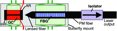
(b)

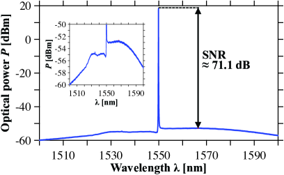
(c)

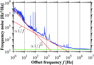
Figure 1: (a) Top-view schematic of the ECDL used in this work. Pads of the butterfly package drawn in red are for current injection to the GC, and those in green are for temperature control. (b) Optical spectrum measured at 525 mA and with $T_{\mathrm{GC}}=T_{\mathrm{FBG}}=$ 20 ^∘C. The inset is close-up view of the amplified spontaneous emission. (c) Corresponding frequency noise. Red lines are proportional to $1/f$ and $1/f^{2}$, respectively, and the green line indicates the white noise floor.

The ECDL design is optimized to provide ULN performance together with extremely stable single-mode operation [36]. The temperature of the GC and of the FBG are independently controlled, which allows for coarse frequency tuning. They are packaged in an extended butterfly mount. The present ECDL does not include any moving parts and its footprint is greatly reduced compared to benchtop ECDLs with a piezo-controlled frequency tuning mechanism [37]. These are inherently less robust, as their cavity alignment is very sensitive to temperature fluctuations and vibrations. A PM optical isolator (OZ Optics) with $\sim$60-dB isolation is spliced to the output fiber to preserve the stability of this device against optical reflections. Note that it has recently been suggested that back reflections from the micro-resonator could be leveraged [38], so that an isolator may not be necessary for soliton generation. This ECDL has a threshold near 40 mA, and an output power of 70 mW was measured after the isolator with a drive current of 525 mA. At this current level, the signal-to-noise ratio (SNR) is $>$70 dB, as seen in Fig. 1(b). The inset of Fig. 1(b) is a close-up view of the amplified spontaneous emission (ASE). On the red side of the lasing peak, the ASE is $\sim$1.5 dB higher than on the blue side. This asymmetry can be understood from the non-linear interaction between the optical field and the carrier density in the QWs [39, 40]. Specifically, the beating between the intense lasing mode and the ASE modulates the (complex) refractive index, which induces extra gain at longer wavelengths.

The frequency noise was measured at 525 mA with an automated system (OEwaves, model OE4000). As seen in Fig. 1(c), a white noise floor of $\sim$20 Hz²/Hz is obtained for frequencies greater than $\sim$10⁶ Hz. This relates [41] to a Lorentzian 3-dB linewidth of $\sim$63 Hz. The low linewidth of this laser is due to its long external cavity length, high storage of photons within this cavity [42], and operation on the long-wavelength side of the FBG reflection [43, 44]. In the frequency range 30 Hz-2 kHz, where the $1/f^{2}$-noise and the $1/f$-noise dominate, several distinct peaks can be seen in Fig. 1(c). They are inherent to the noise from the electronics of the OEwaves measurement system. On the other hand, contributions in the range 1-10 Hz come from the temperature controllers.

RIN measurements were also performed using the OEwaves OE4000 system. Over the entire offset frequency range from 10 Hz to 100 MHz, the measured RIN is equal to the noise floor of the equipment, thus only providing an upper limit to the RIN of the ECDL. The noise floor of the OE4000 unit varies from $-130$ dBc/Hz at 10 Hz, down to almost $-160$ dBc/Hz at 100 kHz, and is then flat out to 100 MHz. This RIN performance is comparable to state-of-the-art low-noise ECDLs in the C band [45], while the linewidth demonstrated by the device in the present experiments is $\sim$15 times narrower.

(a)

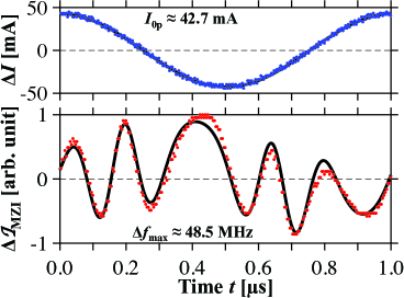
(b)

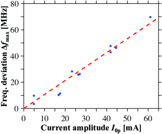
Figure 2: (a) Upper, small-signal current modulation of the ECDL for a certain value of $I_{\mathrm{0p}}$, and lower, intensity out of the MZI fitted (in black) with Eq. (4). (b) Peak frequency deviation $\Delta f_{\max}$ obtained for different current amplitudes $I_{\mathrm{0p}}$. The FM efficiency is extracted from the slope of the linear fit (in red).

To characterize the tuning range, the ECDL output was sent through a fiber-based unbalanced Mach-Zehnder interferometer (MZI) with a free spectral range (FSR) of $\sim$40 MHz. By slowly ramping the current in the ECDL, a normalized frequency change of $\sim$20 MHz/mA is measured, and the widest mode-hop-free tuning range is 2.28 GHz (or 18.3 pm). This is much narrower than specified for benchtop ECDLs, but as will be shown below, the tuning speed is at least 2 orders higher. To characterize the possible tuning speed, a time-harmonic voltage was applied to the ECDL, with a modulation frequency $f_{\mathrm{m}}=\omega_{\mathrm{m}}/(2\pi)$. The current through the ECDL can be expressed as $I(t)=I_{0}+\Delta I(t)$, with a mean value $I_{0}$, a modulation $\Delta I(t)=I_{\mathrm{0p}}\cos\left(\omega_{\mathrm{m}}t\right)$, and a current peak amplitude $I_{\mathrm{0p}}$. This causes the laser frequency to vary harmonically, with a peak deviation $\Delta f_{\max}$. For $f_{\mathrm{m}}\ll\Delta f_{\max}$ and small-signal modulation ($I_{\mathrm{0p}}\ll I_{0}$), the intensity out of the MZI can be written as [27]:

$$\mathfrak{I}_{\mathrm{MZI}}=\mathfrak{I}_{0}+\Delta\mathfrak{I}_{\mathrm{MZI}}=\left(\mathfrak{I}_{0}+\Delta\mathfrak{I}_{\mathrm{IM}}\right)\left(1+\Delta\mathfrak{I}_{\mathrm{FM}}/\mathfrak{I}_{0}\right),$$ (4a)

where $$\mathfrak{I}_{0}$$ is the unmodulated intensity, and:

$$\Delta\mathfrak{I}_{\mathrm{IM}} =m\mathfrak{I}_{0}\cos\left(\omega_{\mathrm{m}}t+\varphi_{\mathrm{IM}}\right)$$ (4b)

$$\Delta\mathfrak{I}_{\mathrm{FM}} =R\mathfrak{I}_{0}\cos\left[2\pi\frac{\Delta f_{\max}}{\mathrm{FSR}}\cos\left(\omega_{\mathrm{m}}t+\varphi_{f}\right)+\varphi_{\mathrm{FM}}\right].$$ (4c)

Eq. (4b) represents the spurious intensity modulation (IM) as the laser frequency is chirped, and $m$ is the IM index. In contrast, Eq. (4c) is used to extract the FM efficiency: $\eta_{\mathrm{FM}}\equiv\Delta f_{\max}/I_{\mathrm{0p}}$. The parameter $R$ is related to the MZI couplers, and the $\varphi$’s are phase constants. In the measurement, the amplitude $I_{\mathrm{0p}}$ is varied up to 61 mA and the modulation frequency is set to $f_{\mathrm{m}}=1$ MHz. Note that for $f_{\mathrm{m}}$ below 50 MHz, temperature-induced FM effects are expected to be significant [46, 47]. Specifically, $\eta_{\mathrm{FM}}$ is expected to decrease as $f_{\mathrm{m}}$ increases from DC to 50 MHz. It is then usually relatively constant up to the relaxation resonance. An example is shown in Fig. 2(a) for $I_{\mathrm{0p}}=42.7$ mA. Fig. 2(b) demonstrates frequency tuning speed above 280 MHz/µs. Significantly, a frequency deviation of 40 MHz (required for soliton generation in a silica micro-disk), can be generated with a current amplitude of 40 mA. Data in Fig. 2(b) are well fitted with a straight line, and the slope is $\eta_{\mathrm{FM}}\approx 1.1$ MHz/mA.

2.3 Silica micro-resonator

The thermally-grown silica micro-disk resonator is fabricated on a Si substrate with a technique reported elsewhere [48]. Its diameter is 3 mm, which corresponds to an FSR of 22 GHz. The resonator profile is a wedge with an angle near 30^∘ and a thickness of 8 µm. This geometry can simultaneously provide anomalous GVD [49, 8], high $Q$ and minimal mode crossing. The latter effect is known to hinder soliton formation [50]. Light is evanescently coupled to the micro-resonator via a tapered fiber [51, 52]. From transmission measurements, the resonance used in this work for soliton generation has a loaded, full-width-at-half-depth (FWHD) linewidth of 1.2 MHz, and therefore a total quality factor $Q_{\scriptsize\mbox{tot}}\approx 160$ M. The micro-resonator was under-coupled in the measurement and had an intrinsic value $Q_{\scriptsize\mbox{i}}\approx 260$ M.

To overcome the thermo-optic effect so that the pump laser frequency is red-detuned relative to the cavity resonance for soliton generation requires rapid tuning over frequency spans as large as 40 MHz at rates in the range of 0.1-2 MHz/µs [15]. This range and rate are readily achievable with the ECDL. As an aside, rates in the range of 0.3-3 MHz/µs are required in SiN combs [16] and also of reach for the ECDL.

2.4 Setup for soliton generation

Fig. 3(a)-(b) shows a schematic of the setup used for soliton generation and locking with the ECDL described in Section 2.2. The ECDL is driven by a low-noise current source (Newport LDX-3620B). A signal generator (SG, Keysight 33522B) produces a local oscillation (LO) used to modulate the voltage supplied to the ECDL, and thereby its emission frequency. The output of the ECDL is connected to a polarization controller (PC, Thorlabs FPC560), and the output of the tapered fiber is connected to a FBG (AOS). Its reflection port (R), with a 0.1-nm pass-band, transmits the pump laser light which is sent to a photo-detector (New Focus 1811, labeled PD₁) and monitored on an oscilloscope. In contrast, the transmission port (T) of the FBG acts as a notch filter and suppresses the pump by 25 dB, so that only the light produced by comb emission and the ASE are detected by PD₂. Part of this photo-current is recorded on the oscilloscope, and the remainder is sent to a servo controller (Vescent D2-125) that subtracts a constant offset. The resulting difference serves as the error signal for a feedback-locking loop [8, 15] essentially based on Eq. (3).

Once the pump frequency reaches the red side of the resonance (prerequisite for soliton generation, see Section 2.1), the SG sends a digital signal to the servo to engage the locking loop. The servo controller includes an op-amp integrator. To establish a stable loop, it forces a null at its input by integrating the error signal within a 10-kHz bandwidth. Its output is a correction voltage signal that is fed back to the ECDL current source, combined with the LO. By adjusting the offset value, states with different soliton numbers can be generated [15]. As shown in the next Section, the tuning and locking parameters were optimized to guarantee the generation and stabilization of a single-soliton state.

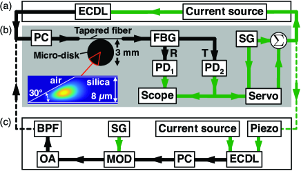
Figure 3: (a)-(b) Schematic of the setup used in this work for soliton generation and locking without an OA. Black and green lines represent optical and electrical paths, respectively. A cross-section schematic of the micro-disk resonator and its wedge profile is shown in (b), with intensity pattern simulated for the fundamental mode. Alternatively, for soliton generation with a piezo-controlled ECDL, part (a) is to be replaced by part (c).

The conventional methods for generation of solitons using piezo-controlled ECDLs can be understood by replacing part (a) with part (c) in Fig. 3. Specifically, two common methods have been developed to overcome the thermal instability and generate solitons. They are based on abrupt changes of either the pump power [8, 15, 9, 16] or the pump frequency [28], and referred to as “power kicking” or “frequency kicking”, respectively. These changes occur over timescales that are faster than the thermal time constant of the micro-resonator. Referring to Fig. 3(c), the pump is typically provided by a benchtop ECDL with a piezo-controlled frequency. The servo feedback is applied to the piezo-controller, and not to the current source like in the procedure described above. For power kicking, the modulator in Fig. 3(c) consists of a combination of acousto-optic and electro-optic modulators (with modulation frequencies up to $\sim$100 MHz). In contrast, the frequency kicking protocol is achieved by manipulating the single sideband from a quadrature phase shift keying (QPSK) modulator driven by a fast-tuning voltage-controlled oscillator (VCO). In both protocols, the modulators are controlled by an extra SG and have optical insertion loss of a few dB. An optical amplifier (OA) is thus inevitably required to boost the pump power. A band-pass filter (BPF) is also preferred to suppress the undesired ASE from the OA. Note that AOMs and QPSKs require a specific polarization for optimal operation, so that an extra PC is also needed. These instruments dramatically increase the footprint, power consumption, and cost of the micro-comb system. In this work, we are able to eliminate these bulky components by implementing a frequency-kicking protocol directly with an ECDL.

3 Results and discussion

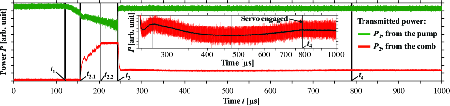
Figure 4: Frequency tuning leading to the generation of a single soliton, and its subsequent locking. The green and the red curves are the transmitted power from the pump and from the comb, respectively. The inset a close-up view of the thermal drift and the soliton locking. The black line is a moving average, and the horizontal scale is logarithmic.

The ECDL is driven at 350 mA where its output power is 42 mW, and the power coupled into the tapered fiber is 34 mW. Fig. 4 shows the evolution of the pump power $P_{1}$ measured after the micro-resonator, as the pump frequency $f_{\scriptsize\mbox{p}}$ is linearly tuned from the blue to the red side of the resonance. Also shown is the generated comb power $P_{2}$. Up to $t_{1}$, $f_{\scriptsize\mbox{p}}$ is so far from resonance that it does not couple significantly to the micro-disk and $P_{1}$ is relatively constant. This situation changes near $t_{1}$ where a reduction of $P_{1}$ is observed as more light couples to the micro-disk. By $t_{2.1}$, the power coupled to the resonator eventually reaches threshold for parametric oscillation, leading to the onset of a primary comb and a sharp increase of $P_{2}$. From $t_{2.1}$ to $t_{3}$, $P_{1}$ further decreases as more pump power is coupled to the resonator, and between $t_{2.2}$ and $t_{3}$, PD₂ is saturated. Heating of the resonator induces the overall triangular-shaped profile of the pump power transmission [31]. Upon arriving at the edge of the blue-detuned side, the pump frequency is kicked a few MHz to the red-detuned side for a few µs, which induces the soliton state in the resonator. Finally, at $t_{4}$, i.e. a few hundred µs after the scanning, the servo loop is engaged to adjust $f_{\scriptsize\mbox{p}}$, so as to lock the soliton state indefinitely against thermal drifting. Variations in $P_{2}$ are further suppressed, suggesting from Eq. (3) that the pump-resonance detuning is indeed stabilized.

(a)

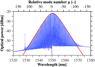
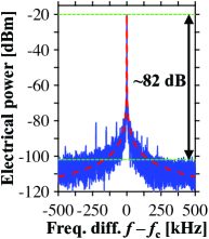
(b) (c)

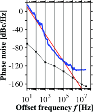
Figure 5: (a) Optical spectrum measured in the single-soliton regime. The red line is a fit according to Eq. (2). (b) Corresponding RF electrical spectrum, with $f_{\mathrm{c}}\approx 22.02$ GHz, fitted with a Lorentzian (in red). The bottom green line indicates the noise level. (c) Phase noise spectral density. The red line is proportional to $1/f^{3}$ and black squares indicate the instrument sensitivity.

To confirm soliton generation, the light output from the T-port of the FBG in Fig. 3(b) is sent to an optical spectrum analyser (OSA, Yokogawa AQ6370). It is seen in Fig. 5(a) that the spectral envelope is relatively smooth, without significant mode crossings. However, an intensity spike with an amplitude 17 dB above the ASE level is centered near 1529 nm (corresponding to a relative mode number $\mu=120$). This spectral feature is a signature of a dispersive wave [53], which can occur from the interaction of the soliton with different transverse modes in the micro-resonator. Eq. (2) provides an excellent fit for the remainder of this spectrum, and leads $\Delta\tau\approx 196$ fs, and $\delta\approx 60$ GHz. The obtained temporal width is within the range of values (125-215 fs) reported in [32]. The value obtained for $\delta$ indicates a red-shifting of the soliton from the pump by nearly 3 FSRs. This self-frequency shift is attributed to the spectral recoil caused by the dispersive wave, and possible stimulated Raman scattering [32, 54, 53]. Here, a single-soliton state is directly generated, in contrast to [55]. No step-like features are visible in the oscilloscope traces of Fig. 4, as these would occur at the transition between different soliton states.

The soliton is further confirmed by assessing the coherence of the generated comb [56]. Indeed, a low-noise and narrow RF signal is known to be a necessary signature of stable soliton formation [6]. The OSA is replaced by a PD (50-GHz bandwidth) connected to an electrical spectrum analyser (ESA, Rohde & Schwarz, FSUP26) that also measures the phase noise. Fig. 5(b) shows the radio-frequency (RF) electrical spectrum recorded with a 100-Hz resolution bandwidth. The carrier frequency $f_{\mathrm{c}}\approx 22$ GHz corresponds to the comb repetition frequency, i.e. to the beating between neighboring comb lines. These data have an SNR $>$80 dB. They are fitted with a Lorentzian, and the 3-dB linewidth is $\sim$25 Hz. Note that the central part is Gaussian with a 3-dB linewidth of $\sim$1.1 kHz.

Finally, Fig. 5(c) shows the phase noise spectral density of the repetition beat note plotted versus the offset frequency $f$. Between 10 Hz and 100 kHz, i.e. over 4 decades, the phase noise is approximately proportional to $1/f^{3}$. This is believed to be contributed by a combination of pump laser RIN and frequency noise [57, 58]. The detected phase noise is smaller than $-100$ dBc/Hz for offset frequencies higher than 28 kHz, which is comparable to the data from a previous report [53], where the silica micro-resonators were pumped with a benchtop ECDL. Beyond 1 MHz, the detected phase noise reaches its floor value of $-129$ dBc/Hz, attributed to the PD shot noise [58].

4 Conclusion

Soliton generation was demonstrated in a micro-resonator with an ultra-low-noise diode laser. A single-soliton state was successfully stabilized by locking the frequency of the pump laser to the power level of the soliton comb. To our knowledge, it is the first time a temporal soliton is realized in a chip-based micro-resonator without an optical amplifier. This demonstration reduces the complexity and cost of soliton experiments, representing a significant step towards soliton comb systems fully integrated on a chip.

Funding Information

This research is supported by a DARPA MTO DODOS contract (HR0011-15-C-055). The views and conclusions contained in this document are those of the authors and should not be interpreted as representing official policies of the Defense Advanced Research Projects Agency or the U.S. Government. N.V. acknowledges support from the Swiss National Science Foundation (SNSF).

References

- [1] T. Udem, J. Reichert, R. Holzwarth, and T. W. Hänsch, \jrPhys. Rev. Lett. 82, 3568–3571 (1999).
- [2] S. A. Diddams, D. J. Jones, J. Ye, S. T. Cundiff, J. L. Hall, J. K. Ranka, R. S. Windeler, R. Holzwarth, T. Udem, and T. W. Hänsch, \jrPhys. Rev. Lett. 84, 5102–5105 (2000).
- [3] D. J. Jones, S. A. Diddams, J. K. Ranka, A. Stentz, R. S. Windeler, J. L. Hall, and S. T. Cundiff, \jrScience 288, 635–639 (2000).
- [4] P. Del’Haye, A. Schliesser, O. Arcizet, T. Wilken, R. Holzwarth, and T. J. Kippenberg, \jrNature 450, 1214–1217 (2007).
- [5] T. J. Kippenberg, R. Holzwarth, and S. A. Diddams, \jrScience 332, 555–559 (2011).
- [6] T. Herr, V. Brasch, J. D. Jost, C. Y. Wang, N. M. Kondratiev, M. L. Gorodetsky, and T. J. Kippenberg, \jrNat. Photon. 8, 145–152 (2014).
- [7] F. Leo, S. Coen, P. Kockaert, S. P. Gorza, P. Emplit, and M. Haelterman, \jrNat. Photon. 4, 471–476 (2010).
- [8] X. Yi, Q. F. Yang, K. Y. Yang, M. G. Suh, and K. Vahala, \jrOptica 2, 1078–1085 (2015).
- [9] V. Brasch, M. Geiselmann, T. Herr, G. Lihachev, M. H. P. Pfeiffer, M. L. Gorodetsky, and T. J. Kippenberg, \jrScience 351, 357–360 (2016).
- [10] S. W. Huang, H. Liu, J. Yang, M. Yu, D. L. Kwong, and C. W. Wong, \jrSci. Rep. 6, 26255 (2016).
- [11] P. H. Wang, J. A. Jaramillo-Villegas, Y. Xuan, X. Xue, C. Bao, D. E. Leaird, M. Qi, and A. M. Weiner, \jrOpt. Express 24, 10890–10897 (2016).
- [12] C. Joshi, J. K. Jang, K. Luke, X. Ji, S. A. Miller, A. Klenner, Y. Okawachi, M. Lipson, and A. L. Gaeta, \jrOpt. Lett. 41, 2565–2568 (2016).
- [13] M. J. R. Heck, J. F. Bauters, M. L. Davenport, J. K. Doylend, S. Jain, G. Kurczveil, S. Srinivasan, Y. Tang, and J. E. Bowers, \jrIEEE J. Sel. Topics Quant. Electron. 19, 6100117 (2013).
- [14] G. Roelkens, A. Abassi, P. Cardile, U. Dave, A. de Groote, Y. de Koninck, S. Dhoore, X. Fu, A. Gassenq, N. Hattasan, Q. Huang, S. Kumari, S. Keyvaninia, B. Kuyken, L. Li, P. Mechet, M. Muneeb, D. Sanchez, H. Shao, T. Spuesens, A. Z. Subramanian, S. Uvin, M. Tassaert, K. van Gasse, J. Verbist, R. Wang, Z. Wang, J. Zhang, J. van Campenhout, X. Yin, J. Bauwelinck, G. Morthier, R. Baets, and D. van Thourhout, \jrPhotonics 3, 969–1004 (2015).
- [15] X. Yi, Q. F. Yang, K. Y. Yang, and K. Vahala, \jrOpt. Lett. 41, 2037–2040 (2016).
- [16] V. Brasch, M. Geiselmann, M. H. P. Pfeiffer, and T. J. Kippenberg, \jrOpt. Express 24, 29312–29320 (2016).
- [17] A. Hasegawa and F. Tappert, \jrAppl. Phys. Lett. 23, 142–144 (1973).
- [18] L. F. Mollenauer, R. H. Stolen, and J. P. Gordon, \jrPhys. Rev. Lett. 45, 1095–1098 (1980).
- [19] T. J. Kippenberg, S. M. Spillane, and K. J. Vahala, \jrPhys. Rev. Lett. 93, 083904 (2004).
- [20] M. G. Suh, Q. F. Yang, K. Y. Yang, X. Yi, and K. J. Vahala, \jrScience 354, 600–603 (2016).
- [21] M. Yu, Y. Okawachi, A. G. Griffith, M. Lipson, and A. L. Gaeta, \jrOpt. Lett. 42, 4442–4445 (2017).
- [22] N. G. Pavlov, G. Lihachev, S. Koptyaev, E. Lucas, M. Karpov, N. M. Kondratiev, I. A. Bilenko, T. J. Kippenberg, and M. L. Gorodetsky, \jrOpt. Lett. 42, 514–517 (2017).
- [23] D. T. Spencer and et al., \jrarXiv:1708.05228 (2017).
- [24] M. G. Suh and K. Vahala, \jrarXiv:1705.06697 (2017).
- [25] P. Trocha, D. Ganin, M. Karpov, M. H. Pfeiffer, A. Kordts, J. Krockenberger, S. Wolf, P. Marin-Palomo, C. Weimann, S. Randel, W. Freude, T. J. Kippenberg, and C. Koos, \jrarXiv:1707.05969 (2017).
- [26] P. Marin-Palomo, J. N. Kemal, M. Karpov, A. Kordts, J. Pfeifle, M. H. P. Pfeiffer, P. Trocha, S. Wolf, V. Brasch, M. H. Anderson, R. Rosenberger, K. Vijayan, W. Freude, T. J. Kippenberg, and C. Koos, \jrNature 546, 274–279 (2017).
- [27] S. Schilt and L. Thévenaz, \jrAppl. Opt. 43, 4446–4453 (2004).
- [28] J. R. Stone, T. C. Briles, T. E. Drake, D. T. Spencer, D. R. Carlson, S. A. Diddams, and S. B. Papp, \jrarXiv:1708.08405 (2017).
- [29] L. A. Lugiato and R. Lefever, \jrPhys. Rev. Lett. 58, 2209–2211 (1987).
- [30] S. Coen and M. Erkintalo, \jrOpt. Lett. 38, 1790–1792 (2013).
- [31] T. Carmon, L. Yang, and K. J. Vahala, \jrOpt. Express 12, 4742–4750 (2004).
- [32] X. Yi, Q. F. Yang, K. Y. Yang, and K. Vahala, \jrOpt. Lett. 41, 3419–3422 (2016). \othercit
- [33] Datasheet available at: www.mortonphotonics.com.
- [34] D. M. Bird, J. R. Armitage, R. Kashyap, R. M. A. Fatah, and K. H. Cameron, \jrElectron. Lett. 27, 1115–1116 (1991).
- [35] P. A. Morton, V. Mizrahi, T. Tanbun-Ek, R. A. Logan, P. J. Lemaire, H. M. Presby, T. Erdogan, S. L. Woodward, J. E. Sipe, M. R. Phillips, A. M. Sergent, and K. W. Wecht, \jrAppl. Phys. Lett. 64, 2634–2636 (1994). \othercit
- [36] P. A. Morton, M. J. Morton, and S. J. Morton, Ultra Low Phase Noise, High Power, Hybrid Lasers for RF Mixing and Optical Sensing Applications, in: IEEE Avionics and Vehicle Fiber-Optics and Photonics Technology Conference (AVFOP), (2017), Paper TuB.1.
- [37] E. C. Cook, P. J. Martin, T. L. Brown-Heft, J. C. Garman, and D. A. Steck, \jrRev. Sci. Instrum. 83, 043101 (2012).
- [38] H. Taheri, A. B. Matsko, and L. Maleki, \jrEur. Phys. J. D 71, 153 (2017).
- [39] A. P. Bogatov, P. G. Eliseev, and B. N. Sverdlov, \jrIEEE J. Quantum Electron. 11, 510–515 (1975).
- [40] H. Kalagara, P. G. Eliseev, and M. Osiński, \jrIEEE J. Sel. Top. Quantum Electron. 19, 1502508 (2013).
- [41] K. Kikuchi and T. Okoshi, \jrIEEE J. Quantum Electron. 21, 669–673 (1985).
- [42] C. H. Henry, \jrIEEE J. Quantum Electron. 19, 1391–1397 (1983).
- [43] R. F. Kazarinov and C. H. Henry, \jrIEEE J. Quantum Electron. 23, 1401–1409 (1987).
- [44] K. Vahala and A. Yariv, \jrAppl. Phys. Lett. 45, 501–503 (1984).
- [45] W. Loh, F. J. O’Donnell, J. J. Plant, M. A. Brattain, L. J. Missaggia, and P. W. Juodawlkis, \jrIEEE Photon. Technol. Lett. 23, 974–976 (2011).
- [46] S. Kobayashi, Y. Yamamoto, M. Ito, and T. Kimura, \jrIEEE J. Quantum Electron. 18, 582–595 (1982).
- [47] J. E. Bowers, W. T. Tsang, T. L. Koch, N. A. Olsson, and R. A. Logan, \jrAppl. Phys. Lett. 46, 233–235 (1985).
- [48] H. Lee, T. Chen, J. Li, K. Y. Yang, S. Jeon, O. Painter, and K. J. Vahala, \jrNat. Photon. 6, 369–373 (2012).
- [49] J. Li, H. Lee, K. Y. Yang, and K. J. Vahala, \jrOpt. Express 20, 26337–26344 (2012).
- [50] T. Herr, V. Brasch, J. D. Jost, I. Mirgorodskiy, G. Lihachev, M. L. Gorodetsky, and T. J. Kippenberg, \jrPhys. Rev. Lett. 113, 123901 (2014).
- [51] M. Cai, O. Painter, and K. J. Vahala, \jrPhys. Rev. Lett. 85, 74–77 (2000).
- [52] S. M. Spillane, T. J. Kippenberg, O. J. Painter, and K. J. Vahala, \jrPhys. Rev. Lett. 91, 043902 (2003).
- [53] X. Yi, Q. F. Yang, X. Zhang, K. Y. Yang, X. Li, and K. Vahala, \jrNat. Commun. 8, 14869 (2017).
- [54] M. Karpov, H. Guo, A. Kordts, V. Brasch, M. H. P. Pfeiffer, M. Zervas, M. Geiselmann, and T. J. Kippenberg, \jrPhys. Rev. Lett. 116, 103902 (2016).
- [55] H. Guo, M. Karpov, E. Lucas, A. Kordts, M. H. P. Pfeiffer, V. Brasch, G. Lihachev, V. E. Lobanov, M. L. Gorodetsky, and T. J. Kippenberg, \jrNature Phys. 13, 94–103 (2017).
- [56] M. Erkintalo and S. Coen, \jrOpt. Lett. 39, 283–286 (2014).
- [57] H. Lee, M. G. Suh, T. Chen, J. Li, S. A. Diddams, and K. J. Vahala, \jrNat. Commun. 4, 1–6 (2013).
- [58] W. Liang, D. Eliyahu, V. S. Ilchenko, A. A. Savchenkov, A. B. Matsko, D. Seidel, and L. Maleki, \jrNat. Commun. 6, 7957 (2015).