The NuSTAR view on Hard-TeV BL Lacs
Abstract
Hard-TeV BL Lacs are a new type of blazars characterized by a hard intrinsic TeV spectrum, locating the peak of their gamma-ray emission in the spectral energy distribution (SED) above 2-10 TeV. Such high energies are problematic for the Compton emission, using a standard one-zone leptonic model. We study six examples of this new type of BL Lacs in the hard X-ray band with NuSTAR. Together with simultaneous observations with the Neil Gehrels Swift Observatory, we fully constrain the peak of the synchrotron emission in their SED, and test the leptonic synchrotron self-Compton (SSC) model. We confirm the extreme nature of 5 objects also in the synchrotron emission. We do not find evidence of additional emission components in the hard X-ray band. We find that a one-zone SSC model can in principle reproduce the extreme properties of both peaks in the SED, from X-ray up to TeV energies, but at the cost of i) extreme electron energies with very low radiative efficiency, ii) conditions heavily out of equipartition (by 3 to 5 orders of magnitude), and iii) not accounting for the simultaneous UV data, which then should belong to a different emission component, possibly the same as the far-IR (WISE) data. We find evidence of this separation of the UV and X-ray emission in at least two objects. In any case, the TeV electrons must not “see” the UV or lower-energy photons, even if coming from different zones/populations, or the increased radiative cooling would steepen the VHE spectrum.
keywords:
BL Lacertae objects: general – radiation mechanisms: non-thermal – gamma-rays: galaxies – X-rays: galaxies1 Introduction
In recent years, a new type of blazar has been discovered through observations at Very High Energies (VHE, 0.1 TeV): the hard-TeV BL Lacs. As any blazar, they are jetted Active Galactic Nuclei (AGN) with the relativistic jet pointing close to the line of sight. Their spectral energy distribution (SED) is characterized by two broad peaks, at low and high energy, commonly explained as synchrotron and inverse Compton (IC) emission from a population of relativistic electrons in the jet. Their SED shows the typical properties of high-energy-peaked BL Lacs (HBL, Padovani & Giommi, 1995): an X-ray band fully dominated by the synchrotron emission, a synchrotron peak frequency above the UV band, and a hard Fermi-LAT spectrum (i.e. photon index 2, Ackermann et al., 2015). Hereafter, we will refer to a spectrum as hard or steep if it is rising or declining with energy in the SED, i.e. if or , respectively.
Their intrinsic VHE emission is characterized by a hard spectrum (1.5 – 1.9) after correction for the effects of - interactions with the diffuse Extragalactic Background Light (EBL), even assuming the lowest possible EBL density provided by galaxy counts (see e.g. Franceschini et al., 2008; Domínguez et al., 2011; Costamante, 2013, and references therein). This locates their Compton peak in the SED assuredly above 2-10 TeV, the highest Compton-peak energies ever seen in blazars (e.g. Aharonian et al., 2006, 2007b, 2007c; Acciari et al., 2009, 2010b).
This is different from all the other VHE-detected HBL, and in particular those bright in Fermi, which are characterized by steep intrinsic VHE spectra () and Compton peak energies around GeV. The SED of these “standard” HBL can be easily reproduced with a one-zone leptonic emission model through the synchrotron self-Compton (SSC) mechanism, using rather standard parameters. A Compton-peak energy above 2-10 TeV becomes instead problematic for standard one-zone leptonic models. The decrease of scattering efficiency in the Klein-Nishina regime tends to steepen the gamma-ray spectrum at VHE, together with the lower energy density of synchrotron seed photons available for scatterings in the Thomson regime, as the energy of electrons increases (see e.g. Fossati et al., 2008; Tavecchio et al., 2010).
Many different alternative scenarios have been proposed: from extremely hard, Maxwellian particle distributions (Saugé & Henri, 2004; Lefa et al., 2011) to a “low-energy” cutoff of the electron distribution at very high energies (Katarzyński et al., 2006; Tavecchio et al., 2009); from internal absorption on a narrow-band radiation field at the source (Aharonian et al., 2008) to a separate origin of the X-ray and TeV emission, the latter coming from kpc-scale jets (Böttcher et al., 2008) or as secondary emission produced by cascades initiated by ultra-high energy (UHE) protons (e.g. Essey & Kusenko, 2010; Essey et al., 2011; Prosekin et al., 2012). The very low flux or upper limits observed in the GeV band with Fermi-LAT (Abdo et al., 2010a; Ackermann et al., 2015) seem now to disfavour internal absorption, at least in these sources. Likewise, relatively fast variability by a factor a few observed at VHE in 1ES 1218304 (on a daily timescale, Acciari et al., 2010a) and 1ES 0229200 (on a yearly timescale, Aliu et al., 2014) seem to disfavour both kpc-scale jets (due to the large sizes) and UHE protons. In the latter case, the deflections in the intergalactic magnetic field and the electromagnetic cascades themselves are expected to introduce long time delays that should smear out such variability, at least up to a few TeV (see e.g. Prosekin et al., 2012; Costamante, 2013).
In the X-ray band, BeppoSAX observations have revealed that HBL can reach synchrotron peak frequencies above a few keV up to and beyond 100 keV, like Mkn 501 during flares (Pian et al., 1998) and 1ES 1426+428 (Costamante et al., 2001). These states/sources were therefore called “extreme synchrotron” BL Lacs (Costamante et al., 2001). Correspondingly, these hard-TeV BL Lacs could be called “extreme Compton” BL Lacs.
Although the two “extreme” properties are expected to be coupled, representing the highest-energy end of the blazar sequence (Ghisellini et al., 1998, 2017), observationally the relation is not yet clear. Some objects do appear extreme in both synchrotron and Compton emissions, such as 1ES 0229+200 (de la Calle Pérez et al., 2003; Kaufmann et al., 2011), 1ES 0347-121 (Aharonian et al., 2007b) and RGB J0710591 (Acciari et al., 2010b). However, there are cases of objects which are extreme only in Compton but not in synchrotron, such as 1ES 1101-232 (Aharonian et al., 2007a), 1ES 1218304 (Acciari et al., 2009) and 1ES 0414009 (Abramowski et al., 2012). Others are extreme in synchrotron but not in Compton, such as 1ES 1426+428 (which is characterized by a steep VHE spectrum after correction for absorption with recent EBL calculations, see e.g. Domínguez et al. 2013).
To reproduce a hard TeV spectrum most scenarios rely on electron distributions with hard features, in the form of “pile-up”, narrow-peaked distributions or low-energy cutoffs at high energy. If true, such spectral features should become visible also in the synchrotron part of the SED, between the UV and hard X-ray bands, because a) the synchrotron emission traces directly the energy distribution of the underlying particle population, and b) the expected fluxes (assuming L LS) are comparable to the observed X-ray flux in these sources. However, they have not been clearly identified so far.
Here we report on a set of coordinated observations in the UV to hard-X-ray bands performed on six hard-TeV BL Lacs, with the satellite NuSTAR (Harrison et al., 2013) and with the X-ray Telescope (XRT, Burrows et al., 2005) and the Ultra-Violet Optical Telescope (UVOT, Roming et al., 2005) on board Swift. The goal is to fully characterize the synchrotron hump in the SED and to identify the synchrotron emission of these putative hard TeV electrons. This emission could appear in the hard X-ray band beyond 10 keV if due to an additional population of electrons, or as a very high X-ray/UV flux ratio, if due to a low-energy cut-off. In the UV band the contribution of the host galaxy is generally negligible (for a typical spectrum of elliptical galaxies), thus the UV photometry should measure directly the non-thermal synchrotron emission from the jet. For all sources we also analyzed the Fermi-LAT data covering the NuSTAR and Swift observations. Together with the VHE data, these measurements allow us to test the viability of the SSC scenario in such extreme conditions.
2 Observations and Data Analysis
The targets were selected on the basis of VHE spectral hardness and highest TeV-peak flux after correction for EBL absorption. In addition to archival data on 1ES 0229+200 (=0.140), the best example of this new class of BL Lacs, new observations were performed on 1ES 0347-121 (=0.188), 1ES 0414009 (=0.287), RGB J0710591 (=0.125), 1ES 1101-232 (=0.186) and 1ES 1218304 (=0.182). In total, we analyzed contemporaneous NuSTAR and Swift observations of six hard-TeV BL Lacs , three of which are characterized historically by hard X-ray spectra, and three by steep X-ray spectra.
The log of the X-ray observations is reported in Table 1. The Swift snapshots mostly overlap with the NuSTAR pointings, covering approximately 10% of the NuSTAR exposure, with the exception of 1ES 0414+009 for which the Swift observation took place 18 hours later. For all sources we checked for variability within and between pointings. No relevant variations were observed (flux variations are limited to a few percent), therefore to improve the statistics on the spectral parameters we considered all the data together, for each source, leaving the cross-normalization between instruments free to vary.
| NuSTAR | SWIFT-XRT | ||||||||
| Object | Obs ID | START | END | Exposure | Obs ID | START | END | Exposure | UVOT |
| [1] | [2] | [3] | [4] | [5] | [6] | [7] | [8] | [9] | [10] |
| 1ES 0229+200 | 60002047002 | 2013-10-02T00:06:07 | 2013-10-02T09:31:07 | 13363 | 00080245001 | 2013-10-01T23:40:23 | 2013-10-01T23:52:54 | 394 | M2 |
| 00080245003 | 2013-10-02T00:49:30 | 2013-10-02T18:41:56 | 2359 | W1 | |||||
| 60002047004 | 2013-10-05T23:31:07 | 2013-10-06T10:16:07 | 19784 | 00080245004 | 2013-10-06T00:56:37 | 2013-10-06T09:11:54 | 5209 | W1 | |
| 60002047006 | 2013-10-10T23:11:07 | 2013-10-11T08:41:07 | 17920 | 00080245005 | 2013-10-10T23:50:32 | 2013-10-10T23:59:56 | 549 | W1 | |
| 00080245006 | 2013-10-11T01:32:11 | 2013-10-11T10:58:56 | 5344 | UU | |||||
| 1ES 0347-121 | 60101036002 | 2015-09-10T04:51:08 | 2015-09-10T22:01:08 | 32802 | 00081692002 | 2015-09-10T06:02:32 | 2015-09-10T12:31:54 | 1965 | W1 |
| 1ES 0414+009 | 60101035002 | 2015-11-25T17:01:08 | 2015-11-26T23:01:08 | 34260a | 00081691001 | 2015-11-27T17:27:16 | 2015-11-27T23:57:55 | 1711 | W2 |
| 22939b | |||||||||
| RGB J0710+591 | 60101037002 | 2015-09-01T05:51:08 | 2015-09-01T07:46:08 | 3386 | 00081693002 | 2015-09-02T00:03:16 | 2015-09-02T03:37:53 | 4427 | all |
| 60101037004 | 2015-09-01T12:11:08 | 2015-09-02T01:31:08 | 26365 | ||||||
| 60101037006 | 2015-09-02T05:51:08 | 2015-09-02T07:56:08 | 4641 | ||||||
| 1ES 1101-232 | 60101033002 | 2016-01-12T21:01:08 | 2016-01-14T01:46:08 | 51522 | 00081689001 | 2016-01-12T22:27:16 | 2016-01-12T22:54:54 | 1633 | W1 |
| 00081689002 | 2016-01-13T00:07:13 | 2016-01-13T02:06:22 | 2854 | UU | |||||
| 1ES 1218+304 | 60101034002 | 2015-11-23T01:06:08 | 2015-11-24T04:11:08 | 49025 | 00081690001 | 2015-11-23T19:39:39 | 2015-11-23T21:26:54 | 1985 | W2 |
| : exposure time with nominal aspect solution (A01 files). | |||||||||
| : exposure time with degraded aspect solution (A06 files), see text. | |||||||||
2.1 NuSTAR observations
Data from both focal plane modules (FPMA & FPMB) onboard the NuSTAR satellite were reprocessed with the NuSTARDAS software package (v1.5.1) jointly developed by the ASI Space Science Data Center (SSDC, Italy) and the California Institute of Technology (Caltech, USA). Event files were calibrated and cleaned with standard filtering criteria with the nupipeline task, using the CALDB version 20150316 and the OPTIMIZED parameter for the exclusion of the SAA passages. We checked the lightcurves for stability of the background, and used the stricter TENTACLE=yes option to exclude intervals with higher/variable background. This was the case only for 1ES 0229+200. We considered only data taken in SCIENCE observing mode, with the exception of 1ES 0414+009 (see below).
Spectra, ancillary and response files were produced using the nuproducts task for pointlike sources, applying corrections for the PSF losses, exposure map and vignetting. The FPMA and FPMB spectra were extracted from the cleaned event files using a circle region of 70–80 arcsec radius, depending on the source intensity, while the background was extracted from nearby circular regions of 80 arcsec radius, on the same chip of the source (after checking the position angle of the pointing). All spectra were binned to ensure a minimum of 20 counts per bin.
When different pointings of the same source were performed, separated by few hours to a few days (like for RGB J0710+591 and 1ES 0229+200), we checked that there were not important differences. To increase the statistics at high energy, we then co-added the spectra for each focal plane module separately, using the task addspec as recommended by NuSTAR science team. This task combines the source and background PHA files as well as the RMF and ARF files.
2.1.1 Specific procedure for 1ES 0414+009
The scientific data corresponding to the SCIENCE observing mode are collected during time intervals in which an aspect solution from the on-board star tracker located on the X-ray optics bench is available. When this solution is not available, the aspect reconstruction is derived using data from the three star trackers located on the spacecraft bus (SCIENCE_SC mode). In this case the accuracy of the sky coordinates degrades to about 2 arcminutes, mainly due to thermal flexing of the spacecraft bus star cameras. Usually the total exposure in this mode is very small compared to the SCIENCE mode (less than 5%), and thus can be filtered out in the standard screening criteria with no significant penalty. However, for the observation of 1ES 0414+009 it amounts to almost half of the exposure (23 ks out of 57 ks). The spectral information in this mode is fully valid, but it is simply spread out (somewhat unevenly) on a wider area. Therefore, to recover this additional exposure, we considered the data in this mode as if coming from an extended source. We extracted the source spectrum from a circle region of radius 120 arcsec, encompassing all the source hotspots, and the background from a circle region of 80 arcsec on the same chip but as far away from the source region as possible, avoiding the chip borders. Response and ancillary files were produced with the extended=yes flag, using the default boxsize=20 value (i.e. the size in pixel for the subimage boxes). We then checked the spectral results of the fits in Xspec against those from the optimal SCIENCE mode, finding no significant difference. We conclude that it is safe to add these spectra to the simultaneous fitting of the total NuSTAR data, with floating cross-normalization parameters, in order to improve the statistical error on the spectral parameters.
Later on we also checked the data with the procedure nusplitsc, newly introduced in NuSTARDAS v1.6.0, which allows the creation of separate spectra with different combinations of star trackers, confirming the results of our previous approach.
2.1.2 Upper limits
The spectral fitting was performed up to energies where the source is detected above 1 sigma (using the command setplot rebin in Xspec). With the exception of 1ES 0229+200, detected over the whole NuSTAR band, the other targets have been detected only up to 30–50 keV. Since our goal is to constrain the presence of additional emission components in the SED, we derived upper limits in the remaining energy range of NuSTAR (up to 79 keV) with the following procedure. We extracted sky images in the undetected energy band with nuproducts, and then summed all images together in XIMAGE (first separately for FPMA and FPMB, and then the total FPMAFPMB images). The total image then corresponds to an FPM image with an exposure time equal to the sum of the FPMA and FPMB times, making full use of the NuSTAR exposure. On this total image, we checked again the absence of the source detection and estimated the background countrate level with XIMAGE tools. We then extracted the 3-sigma upper limit countrate in a circle region of radius 30 arcsec centered on the target position, using the command uplimit in XIMAGE and the Bayesian approach (the prior function is set to the prescription described in Kraft et al. 1991, see XIMAGE user manual). We then converted this countrate value to a flux and SED upper limit with Xspec, by using a power-law model with photon index fixed to , re-normalized to reproduce the measured countrate, and the response and ancillary (effective area) files appropriate for the 30 arcsec extraction region. The upper limit results are reported in Table 2.
| Name | NH,gal | Band | (d.o.f.) | UL | KXRT | |||||
|---|---|---|---|---|---|---|---|---|---|---|
| [1] | [2] | [3] | [4] | [5] | [6] | [7] | [8] | [9] | [10] | [11] |
| 1ES 0229+200 | 9.20 e20 | 0.3–78 | 1.95 e-11 | 1.027 (279) | – | 0.87 | ||||
| 1ES 0347-121 | 3.60 e20 | 0.3–40 | 5.67 e-12 | 0.986 ( 99) | 4.12 e-12 | 0.93 | ||||
| 1ES 0414+009 | 9.15 e20 | 0.3–30 | 7.53 e-12 | 0.997 (180) | 1.53 e-12 | 0.98 | ||||
| RGB J0710+591 | 4.45 e20 | 0.3–50 | 1.71 e-11 | 1.081 (191) | 1.19 e-11 | 1.00 | ||||
| 1ES 1101-232 | 5.76 e20 | 0.3–45 | 2.57 e-11 | 1.016 (253) | 6.37 e-12 | 0.93 | ||||
| 1ES 1218+304 | 1.94 e20 | 0.3–40 | 1.10 e-11 | 0.908 (140) | 3.63 e-12 | 1.13 |
| Name | AB | E(B-V) | ||||||
| 1ES 0229+200 | – | – | – | 0.493 | 0.120 | |||
| 1ES 0347-121 | – | – | – | – | – | 0.167 | 0.040 | |
| 1ES 0414+009 | 0.465 | 0.114 | ||||||
| RGB J0710+591 | 0.139 | 0.034 | ||||||
| 1ES 1101-232 | – | – | – | – | 0.221 | 0.054 | ||
| 1ES 1218+304 | – | – | – | – | – | 0.074 | 0.018 |
2.2 Swift observations
All XRT data were re-processed with standard procedures using the FTOOLS task xrtpipeline. Only data taken in photon counting (PC) mode were considered, representing the bulk of the Swift exposure.
Source events were extracted in the 0.3–10 keV range within a circle of radius 20 pixels (), while background events were extracted from circular and annular regions around the target, free of other sources. When multiple datasets were available, after checking for variability, event files were merged together in XSELECT and the total energy spectrum was extracted from the summed cleaned event file following the same procedure. The ancillary response files were generated with the xrtmkarf task, applying corrections for the PSF losses and CCD defects using the cumulative exposure map. When the source countrate was above 0.5 cts/s, spectra were checked for pile-up problems, and if necessary the central region of the PSF was excised in the spectral extraction. This was the case for RGB J0710+591 (inner 3 arcsec radius), 1ES 1101-232 (7 arcsec) and 1ES 1218+304 (3 arcsec). The source spectra were binned to ensure a minimum of 20 counts per bin.
UVOT observations were performed with the UV filter of the day (see Table 1). Photometry of the source was performed using the UVOT software in the HEASOFT 6.18 package. Counts were extracted from the standard aperture of 5 arcsec radius for all single exposures and all filters, while the background was carefully estimated from different positions more than 27 arcsec away from the source, and avoiding other sources in the field of view. Count rates were then converted to fluxes using the standard zero points (Poole et al., 2008). After checking for variability, all the frames for each filter were summed and a total photometry performed.
For the SED, the fluxes were de-reddened using the mean Galactic interstellar extinction curve from Fitzpatrick (1999), using the values of AB and E(B-V) taken from NED, and reported in Table 3. These are based on the Schlafly & Finkbeiner (2011) recalibration of the Schlegel et al. (1998) infrared-based dust map. For combined UVOT-XRT fits in Xspec, the uvot2pha tool was used, together with the canned response matrices available in the CALDB.
| Name | Epeak(synch) | (synch) | Epeak(Compt) | (Compt) | |||
|---|---|---|---|---|---|---|---|
| [1] | [2] | [3] | [4] | [5] | [6] | [7] | [8] |
| 1ES 0229+200 | 0.140 | 1.31 e-11 | 1.5 | TeV | e-11 | 1.7 | |
| 1ES 0347-121 | 0.188 | 4.17 e-12 | 1.8 | TeV | e-12 | 1.8 | |
| 1ES 0414+009 | 0.287 | 1.13 e-11 | 1.85 | TeV | e-12 | 2.0 | |
| RGB J0710+591 | 0.125 | 1.11 e-11 | 1.85 | TeV | e-12 | 1.8 | |
| 1ES 1101-232 | 0.186 | 1.98 e-11 | 1.7 | TeV | e-11 | 1.7 | |
| 1ES 1218+304 | 0.182 | 8.97 e-12 | 1.9 | TeV | e-11 | 1.9 |
2.3 X-ray spectral analysis
For each source, simultaneous fits of the XRT and NuSTAR spectra were performed using the XSPEC package, using the C-stat statistics adapted for background-subtracted data.
To account for cross-calibration uncertainties between the three telescopes (two NuSTAR and one Swift), a multiplicative constant factor has been included in the spectral model, kept fixed to 1 for NuSTAR/FPMA and free to vary for FPMB and XRT. In the case of FPMB the difference is of the order of 5%, consistent with the expected cross–calibration uncertainty for the instruments (Madsen et al., 2015).
For XRT the difference is of the order of 0-15%, which is slightly larger than the typical inter-calibration uncertainties (). This can be explained with the different exposure times and not fully overlapping epochs, allowing for residual small flux variations. We checked the robustness of the spectral fits also using the cross-calibration obtained by fitting the data in a strictly common energy band (3-9 keV) with a power-law model, finding fully consistent results. For 1ES 0414+009, the FPMA and FPMB datasets taken with degraded aspect solution are included as well, with free constant factors. The differences are again within 5%.
The spectra were fitted with both a single power-law and log-parabolic model, with the ISM absorption model wabs and hydrogen–equivalent column density NH fixed at the Galactic values, as given by the HEASARC tool w3nh using the LAB survey maps (Kalberla et al., 2005).
The only exception is 1ES 0229+200, for which we preferred to use the Dickey & Lockman (DL, Dickey & Lockman, 1990) value of cm-2 (vs ), as a more accurate estimate for the intervening absorption. The reason is that a) the most recent relation of column density vs optical extinction (NH= E(B-V), Liszt, 2014) gives NH values of , closer to the DL estimate; and b) fits with free NH tend to prefer higher NH values of cm-2 than harder power-law models, even using the Swift data alone. Regardless, the Galactic absorption towards 1ES 0229+200 should be considered with a systematic uncertainty in NH between 0.8 and 1.1 cm-2.
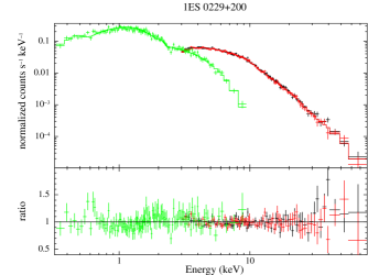
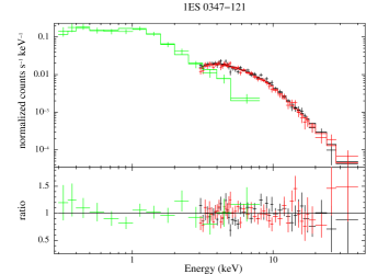
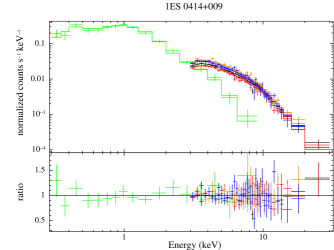
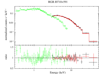
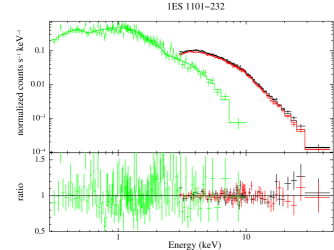
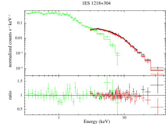
For all objects, a single power-law model does not provide a good fit, showing clear evidence of curvature in the residuals. A log-parabolic model provides a good description of the data in the 0.3–79 keV energy band, and it allows to estimate the error on the position of the synchrotron peak energy (defined as the energy where ) and flux (see e.g. Tramacere et al., 2007). The results of the fits are presented in Table 2, together with the local slopes of the spectrum in the soft (0.3-2 keV) and hard (5-50 keV) X-ray bands. The spectral fits and residuals of the best fit models are shown in Figure 1.
2.4 Fermi-LAT data
We analyzed the data from the LAT detector (Atwood et al., 2009) onboard the Fermi satellite
using the latest Pass 8 data version and the public Fermi Science Tools version v10r0p5.
Given the very low LAT countrate for these objects, we chose to integrate the LAT data over the last 4 years,
from 2013 January 1 to 2016 December 20 (MET 378691203, 503926885). This time interval encompasses
all the NuSTAR pointings of our targets (which occurred between 2013 and 2016),
and provides an homogeneous dataset and time interval over which all targets are detected.
To avoid problems with the strong background at low energies, we selected SOURCE class events in the 0.3-300 GeV range
with gtselect.
Gamma-ray events were selected from a Region of Interest (ROI) of 15°using
standard quality criteria, as recommended by the Fermi Science Support Center (FSSC).
The instrument response functions P8R2_SOURCE_V6 were used.
The Galactic and isotropic diffuse emission were accounted with the models
gll_iem_v06.fits and iso_P8R2_SOURCE_V6_v06.txt, respectively.
| Name | TS | Flux (1-100 GeV) | |
|---|---|---|---|
| [1] | [2] | [3] | [4] |
| 1ES 0229+200 | 56.7 | e-10 | |
| 1ES 0347-121 | 48.8 | e-10 | |
| 1ES 0414+009 | 125.3 | e-10 | |
| RGB J0710+591 | 96.6 | e-10 | |
| 1ES 1101-232 | 63.3 | e-10 | |
| 1ES 1218+304 | 972.1 | e-09 |
Because our time interval does not overlap with the epoch used for the 3FGL catalog,
we performed the likelihood analysis using gtlike in two steps. In the first step, using the tool
make3FGLxml.py we included in the XML model file
all sources in the 3FGL catalog, with free parameters for those within an 8-degree radius from the target or
with free normalization for any source in the ROI flagged as variable in the 3FGL.
We then checked the residual maps –in both counts and Test Statistic (TS, Mattox
et al., 1996)–
for new sources or unmodeled variations of known sources, and changed the XML file accordingly,
identifying and adding sources if TS and dropping all 3FGL sources with a TS in the time interval considered here.
We then performed a second likelihood analysis, using the new optimized XML model file.
The analysis was performed using a binned likelihood with 0.1 deg bins and 10 bins for decade in energy,
with the NEWMINUIT optimizer.
All our targets are detected above 5 in the considered interval. The spectra are well fitted with a single power-law model in the 0.3-300 GeV range. Fit parameters are reported in Table 5. For the SED, the LAT data points were obtained performing a likelihood analysis in each single energy bin, using as model the XML file of the global fit with all parameters fixed to the best-fit values. Only the normalization of the target and of the two backgrounds was left free. A binned or unbinned likelihood was used if the total number of counts in the bin was higher or lower than 1000, respectively. A Bayesian upper limit is calculated if in that bin the target has a TS or npred.
3 Results
All sources show significant curvature in their broad-band X-ray spectrum, which pins down the location of their synchrotron peak in the SED.
The peak energies calculated from the log-parabolic model are reported in Table 4, together with other SED properties constrained by the data: the slope of the spectrum between the UV and soft X-ray (0.3-1 keV) bands, the photon index of the VHE spectrum after correction for EBL absorption (with the model by Franceschini et al., 2008) and the corresponding lower limits on the energy and flux of the Compton peak in the SED.
Five objects present the synchrotron peak directly inside the observed X-ray band, revealing their extreme-synchrotron nature. The peak energy is around 10 keV for 1ES 0229+200, and in the range 1–4 keV for the other four objects. 1ES 0229+200 therefore confirms its most extreme character in the synchrotron as well as Compton emission. It is the only object in our sample detected over the entire NuSTAR band up to 79 keV, and it is also characterized by the hardest slope in the soft X-ray band (, with a systematic uncertainty of due to the uncertainty on the Galactic NH values).
1ES 0414+009 is instead the only object in our sample showing more “standard” HBL properties. Its X-ray spectrum is steep () over the whole band, locating the synchrotron peak energy below or around 0.3 keV (from the curvature of the spectrum).
In all sources there is no evidence of spectral hardening at the highest X-ray energies (see Fig. 1). The NuSTAR data above 10 keV do not show any significant excess above the spectrum determined in the 0.3-10 keV range. The synchrotron emission of the hard-TeV electrons does not seem to provide any significant contribution in the observed hard X-ray band. Therefore any additional emission component in the SED is constrained to appear well above 100 keV.
The UVOT data are generally consistent with the soft X-ray spectrum belonging to the same emission component in the SED. In other words, the slope measured in the soft X-ray band is equal or steeper than the power-law slope connecting the UV to the soft X-ray fluxes ().
However, this is not the case in two objects, namely 1ES 0229+200 and RGB J0710+591. Their soft X-ray spectrum is harder than the UV-to-X-ray slope by about , well above the statistical uncertainty. The UV data therefore remain significantly above the power-law extrapolation of the soft X-ray spectrum towards lower energies. This “UV excess” can either be due to a different synchrotron component, from a different electron population, or could be explained by unaccounted thermal emission from the host galaxy, for example because of a burst of massive star formation caused by a recent merger. However, the additional thermal UV flux required in the latter case would be large, one to two orders of magnitude above the template of a giant elliptical galaxy (Silva et al., 1998, see following section), and therefore we consider this explanation less feasable.
In the gamma-ray band, the Fermi-LAT spectrum match surprisingly well with the VHE spectrum in both flux and slope, after correction for EBL absorption (see Table 4 and 5). The photon indices are similar, in the 1.5–1.8 range. This is the case also for the hardest object, 1ES 0229+200, which shows the same photon index both in the Fermi-LAT and VHE bands. This points toward a Compton peak in the SED well in excess of 10 TeV.
The only exception is represented by 1ES 0414+009. The flat Fermi-LAT spectrum does not seem to belong to the same SED emission component of the VHE data (see Fig. 2). The VHE spectrum appears brighter and harder, though still within the statistical uncertainty. This is one of the weakest BL Lacs detected so far in the VHE band (% of the Crab Nebula flux). However, the LAT spectrum extracted at the beginning of the Fermi mission and partly overlapping with the H.E.S.S. observations (years 2008-2010, see Abramowski et al., 2012) is characterized by a slightly harder photon index and higher flux, more in line with the intrinsic VHE spectrum (Abramowski et al., 2012). We confirm this using Pass 8 data (). We conclude therefore that 1ES 0414+009 has likely changed its gamma-ray SED properties between the two epochs.
4 SED modeling
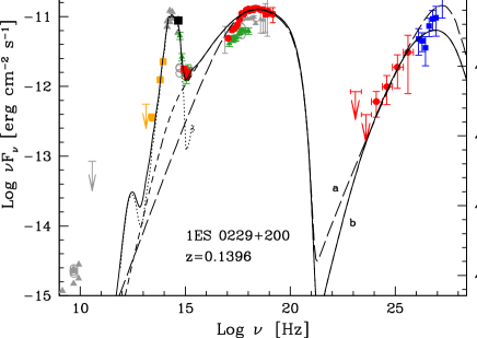
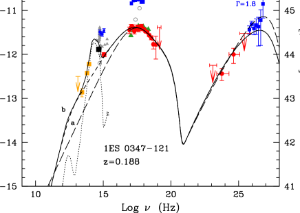
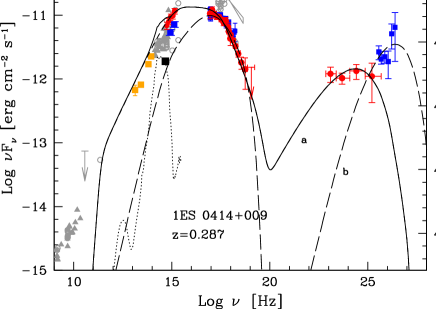
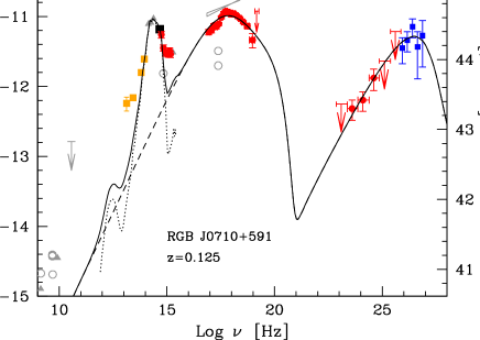
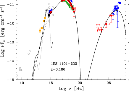
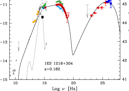
We assembled the SEDs of these BL Lacs complementing our data with archival data from the NASA/IPAC Extragalactic Database (NED), the ASI Space Science Data Center (SSDC) and the Wide-field Infrared Survey Explorer (WISE111Data retrieved from the WISE All–Sky Source Catalog: http://irsa.ipac.caltech.edu/.) satellite (Wright et al., 2010). To account for the presence of the host galaxy –which are typically ellipticals in blazars– we adopted the SED template of a giant elliptical galaxy from Silva et al. (1998), renormalized to match the magnitude of the resolved host galaxy (Scarpa et al., 2000; Falomo & Ulrich, 2000). We corrected the VHE data for the effects of EBL absorption with the model by Franceschini et al. (2008), which agrees well with all present limits and the other recent calculations between UV-Optical and mid infrared wavelengths. The EBL spectrum in its direct stellar component is now well constrained within a narrow band close to the lower limits given by galaxy counts (see e.g. Aharonian et al., 2006; Abdo et al., 2010c; Domínguez et al., 2011; Costamante, 2013). Figure 2 shows the overall SEDs.
We tested the one-zone leptonic SSC scenario using the emission model fully described in Maraschi & Tavecchio (2003). In summary, the emitting region is assumed to be a sphere of radius entangled with uniform magnetic field . The distribution of relativistic electrons is assumed isotropic and follows a smooth broken power law energy spectrum with normalization and indices from to and above the break up to . These electrons emit through synchrotron and SSC mechanisms. The SSC emission is calculated assuming the full Klein-Nishina cross section, which is important in these objects given the high electron energies. Bulk-motion relativistic amplification of the emission is described by the Doppler factor . In total, nine parameters (, , , , , , , , ) fully specify the model.
The theoretical SEDs calculated with this model are plotted in Figure 2, with the corresponding parameters reported in Table 6. To match the gamma-ray data and achieve a Compton peak in the multi-TeV range with sufficient luminosity, the SSC modeling requires extreme energies of the peak electrons, close to 106 , extremely low magnetic fields, at the milliGauss level –implying conditions out of equipartition by 3 to 5 orders of magnitude– and a low density of soft photons in the emitting region. The latter condition is essential in order to avoid efficient cooling of the TeV electrons in the Thomson regime, which would lead to much softer gamma-ray spectra in the VHE range. In a one-zone leptonic scenario, this requires electron distributions with hard low-energy spectra –or low-energy cutoffs– below the X-ray band.
This scenario seems indeed corroborated by our data in the two objects with an “UV excess” (1ES 0229+200 and RGB J0710+591). In these objects the UV flux remains above the extrapolation of the soft X-ray power-law spectrum to lower energies, indicating that they might belong to a different emission component. This is also suggested by the WISE fluxes at the lowest-frequencies, which stay above the host-galaxy emission and can be connected with the UV fluxes as a single power-law emission component (see Fig. 2). The important point is that these two components must not “see” each other: allowing the X-ray electrons to upscatter the observed IR–UV synchrotron photons, whatever their origin, would make impossible to reproduce the gamma-ray data, because of the much softer spectra as a result of the more efficient cooling.
For two other objects, 1ES 0347-121 and 1ES 1101-232, this scenario is not strictly necessary: the UV and X-ray spectra can be fitted with a single synchrotron component (though not the WISE data in 1ES 1101-232). However, the resulting gamma-ray emission tends to slightly underestimate the frequency of the Compton peak with respect to the indication of the VHE spectra (i.e. below 1 TeV instead of above it, though the statistical uncertainty is large). The Compton peak can be better reproduced allowing again for a harder synchrotron spectrum below the X-ray band (compare for example curves a and b in Fig 2).
The remaining two objects 1ES 1218+304 and 1ES 0414+009 are characterized by higher non-thermal emission at optical frequencies, with respect to the other targets. In principle their SED can be fitted using a single electron distribution with three branches (i.e. two breaks). However, as a result the Compton emission peaks at lower energies (Fig. 2). In 1ES 1218+304, it gets underestimated with respect to the best-fit index of the EBL-corrected VERITAS spectrum (, Acciari et al., 2009), by about one decade (below 200 GeV vs above 2 TeV). Given the large statistical uncertainty, a 100-GeV peak energy is still compatible with the data (since at 1), but it would imply that the source is not actually an extreme-Compton BL Lac but a more normal HBL. A Compton peak above 2 TeV would again require a harder synchrotron spectrum which would not account for the observed UV flux.
1ES 0414+009 is characterized by the lowest synchrotron-peak energy and softer X-ray spectrum in our sample. The non-thermal emission at optical frequencies swamps almost completely the host-galaxy flux, and indeed all the WISE and UVOT data appear to stay on a single power-law spectrum. As explained in Sect. 3, this source has most likely changed its Compton peak properties between the VHE and Fermi-LAT epochs. We thus simply accounted for the Fermi-LAT emission as the gamma-ray counterpart of the NuSTAR pointings, obtaining a theoretical SED more in line with standard HBL (curve a in Fig. 2).
However, if one attempts to model the hard VHE spectrum, the model parameters become similar to the ones for other sources (see e.g. curve b in Fig. 2). That is, a much weaker magnetic field and consequently a strong deviation from equipartition. Such a strong change of the magnetic field in the production site might be an important case for the verification of scenarios for the formation of gamma-ray production sites in BL LAC sources.
| Source | ||||||||||||
|---|---|---|---|---|---|---|---|---|---|---|---|---|
| [1] | [2] | [3] | [4] | [5] | [6] | [7] | [8] | [9] | [10] | [11] | [12] | [13] |
| 1ES 0229+200 a | - | - | 50 | |||||||||
| 1ES 0229+200 b | - | - | 50 | |||||||||
| 1ES 0347-121 a | - | - | 60 | |||||||||
| 1ES 0347-121 b | - | - | 60 | |||||||||
| 1ES 0414+009 a | 10 | 1.7 | 20 | 0.5 | ||||||||
| 1ES 0414+009 b | - | - | 60 | |||||||||
| RGB J0710+591 | - | - | 30 | |||||||||
| 1ES 1101-232 a | - | - | 60 | |||||||||
| 1ES 1101-232 b | - | - | 50 | |||||||||
| 1ES 1218+304 | 100 | 1.3 | 50 |
Considering the long integration times of the Fermi-LAT data (4 years) and that the VHE observations took place in general a few years before the Fermi observations, it is somewhat surprising that the LAT and VHE data match so well. There seems to be a striking lack of long-term variability in the gamma-ray emission of these extreme sources.
A likely reason for this lack of large-amplitude variability is that blazars tend to be much less variable at energies below each SED peak than above it (see e.g. Abdo et al., 2010b), the latter corresponding to radiation from freshly accelerated electrons. The flux variations seen in these sources at UV and X-ray energies have been historically much lower than in more typical HBL like Mkn 501 (e.g. Pian et al., 1998; Tavecchio et al., 2001; Aliu et al., 2016a) and Mkn 421 (e.g. Tramacere et al., 2009; Acciari et al., 2014; Kapanadze et al., 2016a; Carnerero et al., 2017), a factor vs or more. Besides, also normal HBL can spend years in low-activity states before undergoing huge flares (e.g. PKS 2155304 in summer 2006, Aharonian et al., 2007d, 2009; Abdalla et al., 2017). Variations of a factor a few in amplitude can remain hidden in the statistical uncertainty and cross-normalization of the gamma-ray datasets considered here.
4.1 Cascades ?
Another possibility is that the gamma-ray band is dominated by secondary emission, arising from the interaction of primary gamma-rays with the diffuse EBL (e.g. Jelley, 1966; Nikishov, 1962; Zdziarski, 1988; Aharonian et al., 1994; Coppi & Aharonian, 1997). The produced electron-positron pairs generate secondary gamma-rays via IC scattering of the Cosmic Microwave Background (CMB), reprocessing primary photons of energy into lower-energy photons of energy GeV (see e.g. Tavecchio et al., 2011).
This interpretation however faces several difficulties for our targets. The cascade scenario can be divided into two main cases: a) both the LAT and the VHE data are dominated by secondaries; b) only the LAT data are dominated by secondaries, while the VHE spectrum measures the primary blazar emission.
In the first case, a secondary emission peaking above 2-10 TeV requires primaries above 50-100 TeV. At such high energies, the mean free path for interactions with the cosmic infrared background is very small, of the order of 10 Mpc or less (Franceschini et al., 2008; Domínguez et al., 2011). At these distances from the AGN the magnetic field is expected to still be rather high ( Gauss) –at the cluster or supercluster level (e.g. Brüggen et al., 2005; Brüggen, 2013)– and thus the pairs are quickly isotropized. These are the typical conditions for the formation of giant pair halos (Aharonian et al., 1994; Eungwanichayapant & Aharonian, 2009). However, studies of the point spread function (PSF) in the H.E.S.S. and VERITAS images of our targets seem to exclude the presence of extended emission (Abramowski et al., 2014; Archambault et al., 2017). Furthermore, the spectrum should be softer than observed below 200 GeV and the intrinsic primary flux is required to be higher than the flux from EBL-correction alone, because of the re-isotropization (Eungwanichayapant & Aharonian, 2009). This would increase dramatically the energy requirements of the source, both in luminosity and peak energy of the primary emission, making the problem of explaining the emitted SED even worse.
The second possibility is that the LAT photons arise from the reprocessing of primary VHE gamma-rays. The intrinsic blazar emission would peak in the TeV range, as in the leptonic SSC scenario. Only one generation of pairs is produced, reprocessing all the absorbed power in the LAT band. The primary emission beam is thus broadened in solid angle by the intergalactic magnetic field (IGMF) acting on the first-generation pairs. The percentage of the absorbed primary flux reaching the observer within the LAT PSF –and thus adding to the primary flux– depends then on the intensity and filling factor of the IGMF along the line of sight (assuming the EBL isotropic). Indeed the Fermi-LAT data of our targets have already been used to put important constraints on the IGMF, at the level of depending on the assumed duration of source activity (Neronov & Vovk, 2010; Tavecchio et al., 2011; Taylor et al., 2011; Finke et al., 2015).
This possibility requires on the one hand a small IGMF (below or close to the derived lower limits) and a very small filling factor, for the secondary emission to be dominant and within the LAT PSF (Ackermann et al., 2013). Both conditions are not granted given the large scale structure of the local Universe (e.g. Costamante, 2013, and references therein). On the other hand, the total amount of absorbed power and the primary spectrum is known, from the observed VHE data and EBL density (Aharonian et al., 2006; Abdo et al., 2010c). This power must emerge in the LAT band on top of any underlying primary GeV emission. The latter therefore must be kept well below the extrapolation of the VHE spectrum into the GeV range, by one to two orders of magnitude. In order not to overproduce the observed LAT data, the primary radiation –and its corresponding electron distribution– must be very narrowly peaked around 2-10 TeV. A narrow electron distribution cannot in general reproduce the full broad-band synchrotron emission in the SED (Lefa et al., 2011). Other electrons could be responsible for different parts of the synchrotron hump, but their SSC emission would again fill the LAT band with primary radiation, unless their SSC flux is suppressed by assuming high magnetic fields in their emitting region. This possibility seems thus less likely due to the extreme fine-tuning and ad-hoc conditions required.
We conclude that, though some contribution from secondary radiation cannot be excluded, it should not be the dominant component of the observed gamma-ray flux.
5 Discussion and Conclusions
The combined NuSTAR and Swift observations provide for the first time three important information for these objects: 1) the precise location of the synchrotron peak in the SED, also for the hardest objects; 2) the relation of the UV flux with respect to the X-ray spectrum; and 3) the absence of a significant hardening of the emission towards higher X-ray energies. The latter result goes against the idea that the hard TeV spectra are produced by an additional electron population, emitting by synchrotron in the hard X-ray band. Their emission is constrained to be well below the observed flux (i.e. implying a high Compton dominance) or at energies much above 100 keV.
Using archival Fermi-LAT and VHE observations, we built the best sampled SED so far for these objects, and tested the one-zone SSC scenario. A leptonic SSC model is able to reproduce the extreme properties of both peaks in the SED quite well, from X-ray up to TeV energies, but at the cost of i) extreme acceleration and very low radiative efficiency, with conditions heavily out of equipartition (by 3 to 5 orders of magnitude); and ii) dropping the requirement to match the simultaneous UV data, which then should belong to a different zone or emission component, possibly the same as the far-IR (WISE) data.
This scenario is corroborated by direct evidence in the X-ray data of 1ES 0229+200 and RGB J0710+591. Their UV flux is in excess of the extrapolation of the soft X-ray spectrum to lower energies. The model can be made to reproduce well either the UV data (over-estimating the soft-X spectrum) or the soft-X spectrum (under-estimating the UV flux), but not both. In the other sources this scenario is not strictly necessary but becomes preferable in order to fully reproduce a Compton peak at multi-TeV energies.
The discrepancy between particle and magnetic energy density is dramatic. Considering a more accurate geometry in the number density of synchrotron photons inside a region of homogeneous emissivity (see Atoyan & Aharonian, 1996) can bring the conditions a factor 3-4 closer to equipartition, but cannot account for orders of magnitude. Remarkably, this discrepancy would not widen significantly in presence of hot protons in the jet, instead of the more common cold assumption. The reason is that the average electron energy in these sources is higher than the rest mass of the proton.
Conditions so far away from equipartition are even more puzzling since not limited to a flaring episode: the extreme nature of the SED in these BL Lacs seem to last for years. If the leptonic scenario is correct, there must be a mechanism which keep the conditions in the dissipation region persistently out of equipartition. The specific case of 1ES 0414+009 shows, however, that some sources could possibly switch closer to equipartition after some years.
In our modeling, the size of the emitting region is of the order of cm with high Doppler factors of 30-60 (see Table 6). These values can accomodate variability on a daily timescale like the one shown by 1ES 1218+304 (Acciari et al., 2010a). In principle, it would be possible to have smaller Doppler factors with larger sizes of the emitting region (for example, in 1ES 0229+200, with cm). However, this solution cannot accomodate variability much faster than a week, and it does not help in bringing the conditions much closer to equipartition (in our example, ).
These hard-TeV BL Lacs represent the extreme case of the more general problem of magnetization in BL Lacs, for which one-zone models imply particle energy and jet kinetic power largely exceeding the magnetic power (see e.g. Tavecchio & Ghisellini, 2016). In these extreme-Compton objects even the assumption of a structured jet –namely a fast spine surrounded by a slower layer– does not help in reaching equipartition. If the layer synchrotron emission is sufficiently broad-banded, the additional energy density in soft photons provided by the layer to the fast-spine electrons does allow for a larger magnetic field and higher IC luminosity, but would generate more efficient cooling of the TeV electrons, preventing a hard spectrum at TeV energies. A spine-layer scenario can thus give solutions close to equipartition for “standard" HBL with a soft TeV spectrum (e.g. Tavecchio & Ghisellini, 2016), but not for these hard-TeV BL Lacs.
The high values of the ratio between the energy density of particles and magnetic field () seems also to exclude magnetic reconnection as possible mechanism for accelerating electrons. At present, relativistic reconnection 2D models predict an upper limit of the order of in the dissipation region (Sironi et al., 2015). The presence of a guiding magnetic field should reduce this ratio even further ().
The NuSTAR and Swift observations of our targets are consistent with the blazar sequence of SED peak frequencies (e.g. Ghisellini et al., 2017), showing a correlation between synchrotron and Compton peak energies. Namely, the highest synchrotron peak frequency and hardest X-ray spectrum are reached in the object with the highest Compton peak energy (1ES 0229200), and vice-versa (1ES 0414+009), with the other four targets clustering around few keV and few TeV for the two SED peaks.
This behaviour is different from standard HBL during strong flares. Standard BL Lacs can show extreme-synchrotron properties in the X-ray band during flares, like for example Mkn 501 in 1997 (Pian et al., 1998; Aharonian et al., 1999; Krawczynski et al., 2002) and 2009 (Aliu et al., 2016b; Ahnen et al., 2016); or 1ES 1959650 in 2002 (Krawczynski et al., 2004) and 2016 (Kapanadze et al., 2016b; Buson et al., 2016). During these flares the synchrotron X-ray emission hardens significantly, shifting the synchrotron peak from below 0.1 keV to 5-10 keV up to 100 keV or more. However, that does not bring a corresponding shift of the Compton peak towards extreme values. The intrinsic VHE emission in those objects remains always steep (), locating the gamma-ray peak in the SED below or around few hundreds GeV (possibly close to TeV only in Mkn 501, in a particular episode, e.g. Ahnen et al., 2016). This might indicate the presence of stronger magnetic fields or generally more efficient cooling during strong dissipative events, as well as the result of a single zone dominating the overall emission from optical to TeV energies.
Given their puzzling emission properties, it is important to find and study more objects of this new type (see e.g. Bonnoli et al., 2015). The extreme-Compton nature is clearly revealed only through VHE observations, by measuring hard TeV spectra after correction for EBL absorption, irrespective of the X-ray or GeV spectra. This requires VHE telescopes with the largest possible collection area and sensitivity in the multi-TeV range, given the typical fluxes of at most few percent of the Crab flux. The upcoming ASTRI (Vercellone et al., 2013) and CTA (Acharya et al., 2013) air-Čerenkov arrays will provide significant progress in this respect.
Acknowledgements
We acknowledge financial support from the CaRiPLo Foundation and the regional Government of Lombardia with ERC for the project ID 2014-1980 “Science and technology at the frontiers of gamma-ray astronomy with imaging atmospheric Cherenkov Telescopes”, and from the agreement ASI-INAF I/037/12/0. We thank Gino Tosti for useful discussions. L. Costamante thanks the Japan Aerospace Exploration Agency (JAXA) for the hospitality and financial support during his visit. This work made use of data from the NuSTAR mission, a project led by the California Institute of Technology, managed by the Jet Propulsion Laboratory, and funded by the National Aeronautics and Space Administration. We thank the NuSTAR Operations, Software and Calibration teams for support with the execution and analysis of these observations. This research has made use of the NuSTAR Data Analysis Software (NuSTARDAS) jointly developed by the ASI Space Science Data Center (SSDC, Italy) and the California Institute of Technology (Caltech, USA). We are grateful to Niel Gehrels and the Swift team for executing and making possible the simultanous observations. This research has made use of the XRT Data Analysis Software (XRTDAS) developed under the responsibility of the ASI Space Science Data Center (SSDC), Italy. Part of this work is based on archival data, software or on-line services provided by SSDC. This research has made use of the NASA/IPAC Extragalactic Database (NED) which is operated by the Jet Propulsion Laboratory, California Institute of Technology, under contract with the National Aeronautics and Space Administration.
We dedicate this paper to Niel Gehrels, who passed away prematurely. His personality and leadership was an essential part of the Swift success. He will always have a special place in our memories.
References
- Abdalla et al. (2017) Abdalla H., et al., 2017, A&A, 598, A39
- Abdo et al. (2010a) Abdo A. A., et al., 2010a, ApJ, 715, 429
- Abdo et al. (2010b) Abdo A. A., et al., 2010b, ApJ, 722, 520
- Abdo et al. (2010c) Abdo A. A., et al., 2010c, ApJ, 723, 1082
- Abramowski et al. (2012) Abramowski A., et al., 2012, A&A, 538, A103
- Abramowski et al. (2014) Abramowski A., et al., 2014, A&A, 562, A145
- Acciari et al. (2009) Acciari V. A., et al., 2009, ApJ, 695, 1370
- Acciari et al. (2010a) Acciari V. A., et al., 2010a, ApJ, 709, L163
- Acciari et al. (2010b) Acciari V. A., et al., 2010b, ApJ, 715, L49
- Acciari et al. (2014) Acciari V. A., et al., 2014, Astroparticle Physics, 54, 1
- Acharya et al. (2013) Acharya B. S., et al., 2013, Astroparticle Physics, 43, 3
- Ackermann et al. (2013) Ackermann M., et al., 2013, ApJ, 765, 54
- Ackermann et al. (2015) Ackermann M., et al., 2015, ApJ, 810, 14
- Aharonian et al. (1994) Aharonian F. A., Coppi P. S., Voelk H. J., 1994, ApJ, 423, L5
- Aharonian et al. (1999) Aharonian F., et al., 1999, A&A, 349, 11
- Aharonian et al. (2006) Aharonian F., et al., 2006, Nature, 440, 1018
- Aharonian et al. (2007a) Aharonian F., et al., 2007a, A&A, 470, 475
- Aharonian et al. (2007b) Aharonian F., et al., 2007b, A&A, 473, L25
- Aharonian et al. (2007c) Aharonian F., et al., 2007c, A&A, 475, L9
- Aharonian et al. (2007d) Aharonian F., et al., 2007d, ApJ, 664, L71
- Aharonian et al. (2008) Aharonian F. A., Khangulyan D., Costamante L., 2008, MNRAS, 387, 1206
- Aharonian et al. (2009) Aharonian F., et al., 2009, A&A, 502, 749
- Ahnen et al. (2016) Ahnen M. L., et al., 2016, preprint, (arXiv:1612.09472)
- Aliu et al. (2014) Aliu E., et al., 2014, ApJ, 782, 13
- Aliu et al. (2016a) Aliu E., et al., 2016a, A&A, 594, A76
- Aliu et al. (2016b) Aliu E., et al., 2016b, A&A, 594, A76
- Archambault et al. (2017) Archambault S., et al., 2017, ApJ, 835, 288
- Atoyan & Aharonian (1996) Atoyan A. M., Aharonian F. A., 1996, MNRAS, 278, 525
- Atwood et al. (2009) Atwood W. B., et al., 2009, ApJ, 697, 1071
- Bonnoli et al. (2015) Bonnoli G., Tavecchio F., Ghisellini G., Sbarrato T., 2015, MNRAS, 451, 611
- Böttcher et al. (2008) Böttcher M., Dermer C. D., Finke J. D., 2008, ApJ, 679, L9
- Brüggen (2013) Brüggen M., 2013, Astronomische Nachrichten, 334, 543
- Brüggen et al. (2005) Brüggen M., Ruszkowski M., Simionescu A., Hoeft M., Dalla Vecchia C., 2005, ApJ, 631, L21
- Burrows et al. (2005) Burrows D. N., et al., 2005, Space Sci. Rev., 120, 165
- Buson et al. (2016) Buson S., Magill J. D., Dorner D., Biland A., Mirzoyan R., Mukherjee R., 2016, The Astronomer’s Telegram, 9010
- Carnerero et al. (2017) Carnerero M. I., et al., 2017, MNRAS, 472, 3789
- Coppi & Aharonian (1997) Coppi P. S., Aharonian F. A., 1997, ApJ, 487, L9
- Costamante (2013) Costamante L., 2013, International Journal of Modern Physics D, 22, 1330025
- Costamante et al. (2001) Costamante L., et al., 2001, A&A, 371, 512
- Dickey & Lockman (1990) Dickey J. M., Lockman F. J., 1990, ARA&A, 28, 215
- Domínguez et al. (2011) Domínguez A., et al., 2011, MNRAS, 410, 2556
- Domínguez et al. (2013) Domínguez A., Finke J. D., Prada F., Primack J. R., Kitaura F. S., Siana B., Paneque D., 2013, ApJ, 770, 77
- Essey & Kusenko (2010) Essey W., Kusenko A., 2010, Astroparticle Physics, 33, 81
- Essey et al. (2011) Essey W., Kalashev O., Kusenko A., Beacom J. F., 2011, ApJ, 731, 51
- Eungwanichayapant & Aharonian (2009) Eungwanichayapant A., Aharonian F., 2009, International Journal of Modern Physics D, 18, 911
- Falomo & Ulrich (2000) Falomo R., Ulrich M.-H., 2000, A&A, 357, 91
- Finke et al. (2015) Finke J. D., Reyes L. C., Georganopoulos M., Reynolds K., Ajello M., Fegan S. J., McCann K., 2015, ApJ, 814, 20
- Fitzpatrick (1999) Fitzpatrick E. L., 1999, PASP, 111, 63
- Fossati et al. (2008) Fossati G., et al., 2008, ApJ, 677, 906
- Franceschini et al. (2008) Franceschini A., Rodighiero G., Vaccari M., 2008, A&A, 487, 837
- Ghisellini et al. (1998) Ghisellini G., Celotti A., Fossati G., Maraschi L., Comastri A., 1998, MNRAS, 301, 451
- Ghisellini et al. (2017) Ghisellini G., Righi C., Costamante L., Tavecchio F., 2017, MNRAS, 469, 255
- Harrison et al. (2013) Harrison F. A., et al., 2013, ApJ, 770, 103
- Jelley (1966) Jelley J. V., 1966, Physical Review Letters, 16, 479
- Kalberla et al. (2005) Kalberla P. M. W., Burton W. B., Hartmann D., Arnal E. M., Bajaja E., Morras R., Pöppel W. G. L., 2005, A&A, 440, 775
- Kapanadze et al. (2016a) Kapanadze B., et al., 2016a, ApJ, 831, 102
- Kapanadze et al. (2016b) Kapanadze B., Dorner D., Kapanadze S., 2016b, The Astronomer’s Telegram, 9205
- Katarzyński et al. (2006) Katarzyński K., Ghisellini G., Tavecchio F., Gracia J., Maraschi L., 2006, MNRAS, 368, L52
- Kaufmann et al. (2011) Kaufmann S., Wagner S. J., Tibolla O., Hauser M., 2011, A&A, 534, A130
- Kraft et al. (1991) Kraft R. P., Burrows D. N., Nousek J. A., 1991, ApJ, 374, 344
- Krawczynski et al. (2002) Krawczynski H., Coppi P. S., Aharonian F., 2002, MNRAS, 336, 721
- Krawczynski et al. (2004) Krawczynski H., et al., 2004, ApJ, 601, 151
- Lefa et al. (2011) Lefa E., Rieger F. M., Aharonian F., 2011, ApJ, 740, 64
- Liszt (2014) Liszt H., 2014, ApJ, 780, 10
- Madsen et al. (2015) Madsen K. K., et al., 2015, ApJS, 220, 8
- Maraschi & Tavecchio (2003) Maraschi L., Tavecchio F., 2003, ApJ, 593, 667
- Mattox et al. (1996) Mattox J. R., et al., 1996, ApJ, 461, 396
- Neronov & Vovk (2010) Neronov A., Vovk I., 2010, Science, 328, 73
- Nikishov (1962) Nikishov A. I., 1962, Soviet Phys. JETP, 14, 393
- Padovani & Giommi (1995) Padovani P., Giommi P., 1995, ApJ, 444, 567
- Pian et al. (1998) Pian E., et al., 1998, ApJ, 492, L17
- Poole et al. (2008) Poole T. S., et al., 2008, MNRAS, 383, 627
- Prosekin et al. (2012) Prosekin A., Essey W., Kusenko A., Aharonian F., 2012, ApJ, 757, 183
- Roming et al. (2005) Roming P. W. A., et al., 2005, Space Sci. Rev., 120, 95
- Saugé & Henri (2004) Saugé L., Henri G., 2004, ApJ, 616, 136
- Scarpa et al. (2000) Scarpa R., Urry C. M., Falomo R., Pesce J. E., Treves A., 2000, ApJ, 532, 740
- Schlafly & Finkbeiner (2011) Schlafly E. F., Finkbeiner D. P., 2011, ApJ, 737, 103
- Schlegel et al. (1998) Schlegel D. J., Finkbeiner D. P., Davis M., 1998, ApJ, 500, 525
- Silva et al. (1998) Silva L., Granato G. L., Bressan A., Danese L., 1998, ApJ, 509, 103
- Sironi et al. (2015) Sironi L., Petropoulou M., Giannios D., 2015, MNRAS, 450, 183
- Tavecchio & Ghisellini (2016) Tavecchio F., Ghisellini G., 2016, MNRAS, 456, 2374
- Tavecchio et al. (2001) Tavecchio F., et al., 2001, ApJ, 554, 725
- Tavecchio et al. (2009) Tavecchio F., Ghisellini G., Ghirlanda G., Costamante L., Franceschini A., 2009, MNRAS, 399, L59
- Tavecchio et al. (2010) Tavecchio F., Ghisellini G., Ghirlanda G., Foschini L., Maraschi L., 2010, MNRAS, 401, 1570
- Tavecchio et al. (2011) Tavecchio F., Ghisellini G., Bonnoli G., Foschini L., 2011, MNRAS, 414, 3566
- Taylor et al. (2011) Taylor A. M., Vovk I., Neronov A., 2011, A&A, 529, A144
- Tramacere et al. (2007) Tramacere A., et al., 2007, A&A, 467, 501
- Tramacere et al. (2009) Tramacere A., Giommi P., Perri M., Verrecchia F., Tosti G., 2009, A&A, 501, 879
- Vercellone et al. (2013) Vercellone S., et al., 2013, preprint, (arXiv:1307.5671)
- Wright et al. (2010) Wright E. L., et al., 2010, AJ, 140, 1868
- Zdziarski (1988) Zdziarski A. A., 1988, ApJ, 335, 786
- de la Calle Pérez et al. (2003) de la Calle Pérez I., et al., 2003, ApJ, 599, 909