Stochastic sampling of quadrature grids for the evaluation of vibrational expectation values

Abstract

The thermal lines method for the evaluation of vibrational expectation values of electronic observables [B. Monserrat, Phys. Rev. B 93, 014302 (2016)] was recently proposed as a physically motivated approximation offering balance between the accuracy of direct Monte Carlo integration and the low computational cost of using local quadratic approximations. In this paper we reformulate thermal lines as a stochastic implementation of quadrature grid integration, analyze the analytical form of its bias, and extend the method to multiple point quadrature grids applicable to any factorizable harmonic or anharmonic nuclear wave function. The bias incurred by thermal lines is found to depend on the local form of the expectation value, and we demonstrate that the use of finer quadrature grids along selected modes can eliminate this bias, while still offering a $\sim 30\%$ lower computational cost than direct Monte Carlo integration in our tests.

I Introduction

First-principles studies of solid state systems typically use the Born-Oppenheimer approximation born_molecules_1929 to simplify the task of solving the Schrödinger equation of the system by separating the electronic and nuclear degrees of freedom. Density functional theory (DFT) jones_dft_2015 is the de facto standard method for solving the electronic problem in crystalline systems, allowing the numerical evaluation of a large number of relevant properties of materials at a relatively low computational cost. The approximate nature of density functionals proves problematic in some cases, and more accurate, computationally costly methods such as the $GW$ approximation Hedin_GW_1965 ; Aryasetiawan_GW_1998 or quantum Monte Carlo ceperley_qmc_1980 ; foulkes_qmc_2001 can be used instead for the evaluation of ground-state observables.

Many electronic properties can usually be evaluated accurately within the static lattice approximation, in which the electronic problem is solved neglecting the effects of nuclear motion entirely. However, zero-point quantum corrections play a crucial role in systems containing light elements, and the description of thermal effects requires the inclusion of vibrations in all systems. The harmonic approximation wallace_thermodynamics_1971 ; born_dynamical_1956 ; maradudin_harmonic_1971 enables the inclusion of nuclear motion for the calculation of the total energy at small computational cost. Although this approach is very accurate for most systems, there are notable exceptions including systems with light atoms, errea_h3s_2016 those involving weak bonding between atoms, fultz_scf3_2011 those at high temperature, Zhao_SnSe_2014 or those near structural phase transitions. trail_tio2_2017 Anharmonic approximations hooton_anharmonic_1958 ; souvatzis_stabilization_2008 ; hellman_anharmonic_2011 ; antolin_free_energy_2012 ; monserrat_anharmonic_2013 ; errea_anharmonicity_2013 exist that are able to overcome these limitations at an additional computational cost.

Vibrational corrections to electronic properties other than the energy can be calculated as the expectation value of the property of interest with respect to the vibrational harmonic or anharmonic nuclear wave function. Literature examples of such calculations include thermal averages of the electronic band structure, allen_band_structure_1981 ; allen_gap_1981 ; giustino_diamond_2010 the dielectric function, williams_1951 ; lax_1952 ; patrick_epsilon_2014 ; zacharias_epsilon_2015 the chemical shielding tensor, rossano_nmr_2005 ; dumez_nmr_2009 ; monserrat_nmr_2014 ; dracinsky_nmr_2014 ; nemausat_nmr_2015 the x-ray absorption near-edge structure, nemausat_nmr_2015 or the contact hyperfine interaction. porter_muon_1999 ; moller_muon_2013 These vibrational averages have traditionally been computed using either a quadratic expansion of the electronic observable around its equilibrium value, or Monte Carlo integration. The former approach is computationally advantageous, but neglects multi-phonon terms in the electron-phonon interaction. The latter approach is computationally costly, but multi-phonon terms are correctly captured. The recent demonstration that multi-phonon terms can be important in a number of cases monserrat_helium_2014 ; monserrat_giant_2015 ; patrick_cssni3_2015 ; saidi_mapbi3_2016 has motivated the development of the thermal lines method, monserrat_TL_2016 which can partially capture multi-phonon terms at a smaller computational cost than Monte Carlo integration.

The thermal lines method was proposed as a physically-motivated approximation to the evaluation of vibrational expectation values of electronic observables, offering faster statistical convergence than Monte Carlo integration and better accuracy than the quadratic approximation, but its bias has not yet been quantified. In the present paper we analyze the bias of the thermal lines method, and use this analysis to propose an integration method based on the stochastic sampling of quadrature grids constructed from the vibrational wave function. The bias in our proposed method is controlled by the number of grid points, reducing to thermal lines for a two-point grid and to Monte Carlo integration in the infinite-point limit. Our results indicate that thermal lines (two-point grids) are capable of accurately incorporating the effects of multi-phonon terms in most calculations of vibrational expectation values. However, we find that the bias incurred by thermal lines is not negligible for observables with a strong non-quadratic behavior, and multiple point grids are required in order to obtain accurate expectation values in these cases.

The rest of this paper is structured as follows. In section II we provide the theoretical background and describe the relevant methods for the evaluation of vibrational expectation values. The bias in the thermal lines method is analyzed in section III. In section IV we formulate and test one-dimensional quadrature grids, and in section V we discuss the use of these grids in multi-dimensional Monte Carlo sampling for realistic examples of vibrational averages of electronic observables. Finally, we summarize our findings in section VI. Hartree atomic units ($\hbar=|e|=m_{\rm e}=4\pi\epsilon_{0}=1$) are used throughout.

II Vibrational calculations

In computer simulations, crystalline solids are represented by supercells containing $N$ nuclei and $N_{e}$ electrons subject to periodic boundary conditions. Within the Born-Oppenheimer approximation, the electronic Hamiltonian ${\hat{H}}_{\rm el}({\bf R})$ parametrically depends on the nuclear positions ${\bf R}$, and the resulting electronic energy $E_{\rm el}({\bf R})$, in which we include nucleus-nucleus interactions, acts as an external potential in the vibrational Hamiltonian,

$${\hat{H}}_{\rm vib}({\bf R})=-\sum_{\alpha=1}^{N}\frac{1}{2m_{\alpha}}\nabla_{\alpha}^{2}+E_{\rm el}({\bf R})\;.$$ (1)

Without loss of generality we will assume that $E_{\rm el}({\bf R}_{0})=0$, where ${\bf R}_{0}$ is the equilibrium nuclear configuration. The nuclear motion problem has three translational degrees of freedom which can be eliminated, and $n=3N-3$ vibrational degrees of freedom.

It is convenient to work in terms of normal-mode coordinates ${\bf u}=\{u_{i}\}_{i=1}^{n}$, which are the real-valued linear combinations of nuclear displacements under which the dynamical matrix is diagonal. wallace_thermodynamics_1971 ; born_dynamical_1956 ; maradudin_harmonic_1971 We replace the phonon branch $\nu$ and wave vector ${\bf q}$, which are the standard normal mode quantum numbers, by a single index $i$ for notational convenience. Note that ${\bf u}={\bf 0}$ at the equilibrium nuclear configuration ${\bf R}_{0}$. In these coordinates, Eq. 1 reads

$${\hat{H}}_{\rm vib}({\bf u})=-\frac{1}{2}\sum_{i=1}^{n}\frac{\partial^{2}}{\partial u_{i}^{2}}+E_{\rm el}({\bf u})\;.$$ (2)

The ground-state vibrational wave function $\Phi({\bf u})$ determines the zero-temperature quantum vibrational properties of the system, and can be obtained by solving the vibrational Schrödinger equation, ${\hat{H}}_{\rm vib}({\bf u})\Phi({\bf u})=E_{\rm vib}\Phi({\bf u})$.

Under the harmonic approximation, the electronic energy is assumed to take the form $E_{\rm el}({\bf u})=\sum_{i}\frac{1}{2}\omega_{i}u_{i}^{2}$, where the harmonic frequency of the $i$th normal mode $\omega_{i}$ can be obtained by differentiating the electronic energy, either using finite differences fd_kunc_1982 ; nondiagonal_lloydwilliams_2015 or methods such as density functional perturbation theory, baroni_dfpt_2001 with respect to $u_{i}$. The harmonic approximation results in a wave function of the form $\Phi^{\rm(har)}({\bf u})=\prod_{i=1}^{n}\phi^{(\rm har)}_{i}(u_{i})$, where

$$\phi^{\rm(har)}_{i}(u_{i})=\left(\frac{\omega_{i}}{\pi}\right)^{1/4}\exp\left(-\frac{1}{2}\omega_{i}u_{i}^{2}\right)\;.$$ (3)

Various methods for dealing with anharmonic vibrational Hamiltonians exist which lift the restriction on the form of the electronic energy, souvatzis_stabilization_2008 ; hellman_anharmonic_2011 ; antolin_free_energy_2012 ; monserrat_anharmonic_2013 ; errea_anharmonicity_2013 but all these methods assume that the wave function can be factorized as a product of single-mode functions, $\Phi({\bf u})=\prod_{i=1}^{n}\phi_{i}(u_{i})$. In our analysis we assume the use of a factorizable vibrational wave function.

We focus our present discussion on the zero-temperature limit for simplicity. Thermal effects can be trivially including by replacing the ground-state vibrational density $\Phi^{2}$ with $\frac{1}{\cal Z}\sum_{\bf s}\Phi_{\bf s}^{2}e^{\beta E_{\bf s}}$, where $\beta=({k_{\rm B}T})^{-1}$ is the inverse temperature, $\bf s$ identifies the vibrational excited state corresponding to wave function $\Phi_{\bf s}$ and energy $E_{\bf s}$, and ${\cal Z}=\sum_{\bf s}e^{\beta E_{\bf s}}$ is the partition function of the system. We note that the “mean thermal line” approach for evaluating finite-temperature expectation values monserrat_TL_2016 remains applicable to our proposed method.

II.1 Vibrational expectation values

Knowledge of $\Phi({\bf u})$ enables the evaluation of the expectation value of an electronic observable $\hat{A}$ with respect to the vibrational density as

$$\langle A\rangle_{\Phi^{2}}=\int\Phi^{2}({\bf u})A({\bf u})\,{\rm d}{\bf u}\;,$$ (4)

where $A({\bf u})=\Phi^{-1}({\bf u}){\hat{A}}\Phi({\bf u})$ is the local value of the observable at nuclear configuration $\bf u$. Under the assumption that $A({\bf u})$ is a smooth function of its arguments, it is useful to express it as a power expansion,

$$A({\bf u}) = A({\bf 0})+\sum_{i}^{n}a_{i}^{(1)}u_{i}+\sum_{i\leq j}^{n}a_{ij}^{(2)}u_{i}u_{j}$$ (5)

$$+ \sum_{i\leq j\leq k}^{n}a_{ijk}^{(3)}u_{i}u_{j}u_{k}+\ldots\;,$$

where $a_{i}^{(1)}$, $a_{ij}^{(2)}$, $a_{ijk}^{(3)}$, etc., are linear expansion coefficients. It should be noted that the approximations involved in solving the vibrational Schrödinger equation are distinct from those applied to $A({\bf u})$; namely, the use of the harmonic wave function does not imply that expectation values are assumed to be quadratic functions of $\bf u$ (or vice versa), and the use of a factorizable wave function without explicit phonon-phonon correlations does not imply neglecting multi-mode contributions from Eq. 5 (or vice versa). antonius_anh_2015

II.1.1 The quadratic approximation

If $\Phi({\bf u})$ is symmetric, such as in the harmonic approximation, substituting Eq. 5 into Eq. 4 results in the cancellation of all contributions involving odd powers of a normal-mode coordinate,

$$\langle A\rangle_{\Phi^{2}} = A({\bf 0})+\sum_{i}^{n}a_{ii}^{(2)}\langle u_{i}^{2}\rangle_{\Phi^{2}}+\sum_{i\leq j}^{n}a_{iijj}^{(4)}\langle u_{i}^{2}u_{j}^{2}\rangle_{\Phi^{2}}$$

$$+ \sum_{i\leq j\leq k}^{n}a_{iijjkk}^{(6)}\langle u_{i}^{2}u_{j}^{2}u_{k}^{2}\rangle_{\Phi^{2}}+\ldots\;,$$ (6)

and since $\Phi^{2}$ is factorizable, Eq. 6 reduces to a linear combination of products of one-dimensional integrals. Neglecting fourth- and higher-order contributions to Eq. 6 yields the quadratic approximation,

$$\langle A\rangle_{\Phi^{2}}\approx A({\bf 0})+\sum_{i}^{n}a_{ii}^{(2)}\langle u_{i}^{2}\rangle_{\phi_{i}^{2}}\;,$$ (7)

where $a_{ii}^{(2)}=\frac{1}{2}\left(\frac{\partial^{2}A}{\partial u_{i}^{2}}\right)_{{\bf u}={\bf 0}}$, and the one-dimensional integrals $\langle u_{i}^{2}\rangle_{\phi_{i}^{2}}$ can easily be calculated; in the harmonic approximation, $\langle u_{i}^{2}\rangle_{\phi_{i}^{2}}=(2\omega_{i})^{-1}$.

II.1.2 Direct Monte Carlo integration

An unbiased estimate of the integral of Eq. 4 can be evaluated using Monte Carlo integration,

$$\langle A\rangle_{\Phi^{2}}\approx\frac{1}{M}\sum_{m=1}^{M}A({\bf u}_{m})\;,$$ (8)

where $\{{\bf u}_{m}\}$ are $M$ random vectors of normal-mode coordinates distributed according to $\Phi^{2}({\bf u})$. This method, which we refer to as direct Monte Carlo in what follows, is exact in the limit $M\to\infty$, and requires no assumptions about the form of $A({\bf u})$ or $\Phi({\bf u})$. However, if the wave function is symmetric about ${\bf u}={\bf 0}$, $\Phi({\bf u})=\Phi(-{\bf u})$, it is advantageous to accumulate samples in {${\bf u}$, $-{\bf u}$} pairs in order to exactly remove odd-order contributions,

$$A^{*}({\bf u}) = \frac{1}{2}[A({\bf u})+A(-{\bf u})]$$ (9)

$$= A({\bf 0})+\sum_{i\leq j}^{n}a_{ij}^{(2)}u_{i}u_{j}$$

$$+ \sum_{i\leq j\leq k\leq l}^{n}a_{ijkl}^{(4)}u_{i}u_{j}u_{k}u_{l}+\ldots\;,$$

resulting in reduced random noise and faster statistical convergence, while giving the correct expectation value since it is trivial that $\langle A({\bf u})\rangle_{\Phi^{2}}=\langle A^{*}({\bf u})\rangle_{\Phi^{2}}$. This sampling strategy, which we refer to as symmetrized sampling, was used in Ref. monserrat_TL_2016, for the “TL₂” variant of the thermal lines method, but it can be used to accelerate any Monte Carlo evaluation of the expectation value of $\hat{A}$ with a symmetric wave function.

II.1.3 Thermal lines

Inspired by the mean value theorem for integrals, the thermal lines method monserrat_TL_2016 postulates that a good approximation to the expectation value of $\hat{A}$ for a symmetric wave function is given by

$$\langle A\rangle_{\Phi^{2}}\approx\frac{1}{M}\sum_{m=1}^{M}A[{\bf u}_{\rm TL}({\bf S}_{m})]\;,$$ (10)

where $\{{\bf S}_{m}\}$ are $M$ random $n$-dimensional vectors each of whose components takes the values $+1$ and $-1$ with equal probability, and ${\bf u}_{\rm TL}({\bf S})$ is a vector whose $i$th component is $S_{i}U_{i}$, where $U_{i}=\sqrt{\langle u_{i}^{2}\rangle_{\Phi^{2}}}$.

The thermal lines method defines “special” points at which to sample the integrand, much in the spirit of special $k$-point methods for integrals over the Brillouin zone of a crystal, baldereschi_integration_1973 ; rajagopal_specialk_1994 or quadrature grids for integrals over the surface of a sphere, lebedev_quadrature_1976 ; reeger_quadrature_2015 and uses Monte Carlo sampling of these points to efficiently deal with the high dimensionality of the integration volume. Although the effectiveness of thermal lines for the calculation of vibrational averages was demonstrated in Ref. monserrat_TL_2016, , there was no formal analysis of the bias incurred by replacing Eq. 8 by Eq. 10. We present such analysis in section III.

We note that Monte Carlo sampling over thermal lines has been used to study the effects of electron-phonon coupling on the temperature dependence of the band gaps of a number of semiconductors within the $GW$ approximation Monserrat_GW_2016 and to study phonon-assisted optical absorption in BaSnO₃ using a hybrid DFT functional. Monserrat_BaSnO3_2017 It has also been shown that, in the thermodynamic limit $n\to\infty$, a single thermal line delivers the exact thermal average $\langle A\rangle_{\Phi^{2}}$ without the need of Monte Carlo sampling. This thermal line is such that the sign $S_{i}$ alternates between $+1$ and $-1$ when the coordinates $u_{i}$ are ordered by increasing value of their associated harmonic frequencies $\omega_{i}$. zacharias_one-shot_2016 Finally, we note that other methods in the same spirit as thermal lines have been used, for example in the study of superconducting hydrogen sulfides. Komelj_H3S_2015

III Analysis of thermal lines

The distribution of normal-mode configurations $\bf u$ sampled in Eq. 10 can be identified with the following probability density function,

$$\Phi^{2}_{\rm TL}({\bf u})=\frac{1}{2^{n}}\prod_{i=1}^{n}\left[\delta(u_{i}-U_{i})+\delta(u_{i}+U_{i})\right]\;,$$ (11)

where $\Phi_{\rm TL}$ is the “thermal lines wave function”. At ${\bf u}_{\rm TL}=\left\{S_{i}U_{i}\right\}$, Eq. 5 becomes

$$A({\bf u}_{\rm TL}) = A({\bf 0})+\sum_{i=1}^{n}a_{i}^{(1)}S_{i}U_{i}+\sum_{i\leq j}^{n}a_{ij}^{(2)}S_{i}S_{j}U_{i}U_{j}$$ (12)

$$+ \sum_{i\leq j\leq k}^{n}a_{ijk}^{(3)}S_{i}S_{j}S_{k}U_{i}U_{j}U_{k}$$

$$+ \sum_{i\leq j\leq k\leq l}^{n}a_{ijkl}^{(4)}S_{i}S_{j}S_{k}S_{l}U_{i}U_{j}U_{k}U_{l}+\ldots\;.$$

The expectation value of products of powers of $S$ for different modes factorizes into products of single-mode expectation values, e.g., $\langle S_{i}^{\beta}S_{j}^{\gamma}\rangle=\langle S_{i}^{\beta}\rangle\langle S_{j}^{\gamma}\rangle$ for $i\neq j$, and each of these is zero if the exponent is odd and unity if the exponent is even. The expectation value of $\hat{A}$ under the thermal lines wave function is therefore

$$\langle A\rangle_{\Phi_{\rm TL}^{2}} = A({\bf 0})+\sum_{i}^{n}a_{ii}^{(2)}U_{i}^{2}+\sum_{i\leq j}^{n}a_{iijj}^{(4)}U_{i}^{2}U_{j}^{2}$$ (13)

$$+ \sum_{i\leq j\leq k}^{n}a_{iijjkk}^{(6)}U_{i}^{2}U_{j}^{2}U_{k}^{2}+\ldots\;,$$

which agrees with the quadratic approximation to second order, but includes higher-order multi-mode contributions. Subtracting Eq. 13 from Eq. 6 and substituting $U_{i}^{2}=\langle u_{i}^{2}\rangle_{\Phi^{2}}$, the bias in the thermal lines expectation value is

$$\langle A\rangle_{\Phi^{2}}-\langle A\rangle_{\Phi_{\rm TL}^{2}} = \sum_{i}^{n}a_{iiii}^{(4)}\left(\langle u_{i}^{4}\rangle_{\Phi^{2}}-\langle u_{i}^{2}\rangle_{\Phi^{2}}^{2}\right)$$ (14)

$$+ \sum_{i}^{n}a_{iiiiii}^{(6)}\left(\langle u_{i}^{6}\rangle_{\Phi^{2}}-\langle u_{i}^{2}\rangle_{\Phi^{2}}^{3}\right)$$

$$+ \sum_{i<j}^{n}a_{iiiijj}^{(6)}\left(\langle u_{i}^{4}\rangle_{\Phi^{2}}-\langle u_{i}^{2}\rangle_{\Phi^{2}}^{2}\right)\langle u_{j}^{2}\rangle_{\Phi^{2}}$$

$$+ \sum_{i<j}^{n}a_{iijjjj}^{(6)}\langle u_{i}^{2}\rangle_{\Phi^{2}}\left(\langle u_{j}^{4}\rangle_{\Phi^{2}}-\langle u_{j}^{2}\rangle_{\Phi^{2}}^{2}\right)$$

$$+ {\cal O}(u^{8})\;.$$

It should be noted that the bias in the quadratic approximation includes all fourth- and higher-order terms in Eq. 6, while Eq. 14 shows that the bias in thermal lines arises solely from terms of fourth or higher order in which all index values appear an even number of times. Therefore the bias in thermal lines expectation values can typically be expected to be smaller than that for the quadratic approximation.

The variance of the values of $A({\bf u})$ encountered during Monte Carlo integration determines the statistical uncertainty of the result. The sample variance ${\rm var}[A]=\left\langle\left(A-\langle A\rangle\right)^{2}\right\rangle$ associated with the $\Phi^{2}$ distribution is

$${\rm var}_{\Phi^{2}}[A] = \sum_{i=1}^{n}{a_{i}^{(1)}}^{2}\langle u_{i}^{2}\rangle_{\Phi^{2}}$$ (15)

$$+ \sum_{i=1}^{n}{a_{ii}^{(2)}}^{2}\left(\langle u_{i}^{4}\rangle_{\Phi^{2}}-\langle u_{i}^{2}\rangle_{\Phi^{2}}^{2}\right)$$

$$+ \sum_{i<j}^{n}{a_{ij}^{(2)}}^{2}\langle u_{i}^{2}\rangle_{\Phi^{2}}\langle u_{j}^{2}\rangle_{\Phi^{2}}$$

$$+ \sum_{i=1}^{n}a_{i}^{(1)}a_{iii}^{(3)}\langle u_{i}^{4}\rangle_{\Phi^{2}}$$

$$+ \sum_{i<j}^{n}\left(a_{i}^{(1)}a_{iij}^{(3)}+a_{j}^{(1)}a_{ijj}^{(3)}\right)\langle u_{i}^{2}\rangle_{\Phi^{2}}^{2}\langle u_{j}^{2}\rangle_{\Phi^{2}}^{2}$$

$$+ {\cal O}(u^{6})\;.$$

The expression for ${\rm var}_{\Phi_{\rm TL}^{2}}[A]$ is similar to Eq. 15, but replacing $\langle u_{i}^{4}\rangle_{\Phi^{2}}$ with $\langle u_{i}^{2}\rangle_{\Phi^{2}}^{2}$, which eliminates the second term. The leading order contribution to both ${\rm var}_{\Phi^{2}}[A]$ and ${\rm var}_{\Phi_{\rm TL}^{2}}[A]$ is thus due to the asymmetry of the expectation value along individual modes. We note that there exist observables for which the thermal lines method gives a greater variance than direct Monte Carlo integration. For example, for a one-dimensional harmonic wave function of frequency $\omega=1$ the function $A(u)=-3u+u^{2}+u^{3}$ is sampled with greater variance with unsymmetrized-sampling thermal lines than with unsymmetrized-sampling direct Monte Carlo. However, in the absence of asymmetries, the cancellation of the second term in Eq. 15 implies that ${\rm var}_{\Phi_{\rm TL}^{2}}[A]<{\rm var}_{\Phi^{2}}[A]$ to leading order.

The variance of $A^{*}$ can be obtained from Eq. 15 by zeroing the $a$ coefficients of odd-order terms, so only the second and third terms survive in ${\rm var}_{\Phi^{2}}[A^{*}]$, and only the third term survives in ${\rm var}_{\Phi_{\rm TL}^{2}}[A^{*}]$. Thus, the variance from symmetrized-sampling thermal lines is identically zero in one dimension, and in multiple dimensions the sample variance arises solely from multi-mode contributions. By contrast, ${\rm var}_{\Phi^{2}}[A^{*}]$ contains single-mode contributions, hence ${\rm var}_{\Phi_{\rm TL}^{2}}[A^{*}]<{\rm var}_{\Phi^{2}}[A^{*}]$ to leading order.

The thermal lines method combines the construction of a one-dimensional two-point integration grid with $n$-dimensional Monte Carlo sampling, and it is useful to analyze these two aspects of the method separately. If stochastic sampling is ignored, thermal lines reduces to quadrature integration; in fact, the thermal lines grid for the harmonic wave function is a two-point Gauss-Hermite quadrature grid. Abramowitz_1965 In the following, we generalize thermal lines by formulating one-dimensional quadrature grids adapted to the single-mode wave function in Section IV, and then we separately discuss the $n$-dimensional Monte Carlo sampling of these grids in Section V.

IV One-dimensional quadrature grids

We define our quadrature grids as an approximation to the integral

$$\langle A\rangle_{\phi^{2}}=\int_{-\infty}^{\infty}\phi^{2}(u)A(u)\,{\rm d}u\approx\sum_{\alpha=1}^{p}P_{\alpha}A(U_{\alpha})\;,$$ (16)

where $p$ is the number of points in the grid, $U_{\alpha}$ is the $\alpha$th grid point, and $P_{\alpha}$ is its corresponding weight, which satisfies $\sum_{\alpha=1}^{p}P_{\alpha}=1$. This approximation is equivalent to replacing $\phi^{2}(u)$ in Eq. 16 with the discrete probability distribution

$$\psi_{p}^{2}(u)=\sum_{\alpha=1}^{p}P_{\alpha}\delta(u-U_{\alpha})\;,$$ (17)

so that the right-hand side of Eq. 16 is $\langle A\rangle_{\psi_{p}^{2}}$. Note that when $p\to\infty$ Eq. 17 must reduce to the full single-mode probability distribution, $\lim_{p\to\infty}P_{\alpha}\propto\phi^{2}(U_{\alpha})$.

A $p$-point quadrature grid has $2p$ unknowns, which we determine by imposing that the quadrature integral be exact for a polynomial of order $2p-1$. Let

$$A(u)=\sum_{\beta=0}^{2p-1}a_{\beta}u^{\beta}\;.$$ (18)

The left-hand side of Eq. 16 is then

$$\langle A\rangle_{\phi^{2}}=\sum_{\beta=0}^{2p-1}a_{\beta}\langle u^{\beta}\rangle_{\phi^{2}}=\sum_{\beta=0}^{2p-1}a_{\beta}\mu_{\beta}\;,$$ (19)

where $\mu_{\beta}=\langle u^{\beta}\rangle_{\phi^{2}}$ is the $\beta$th moment of $\phi^{2}$, and the right-hand side of Eq. 16 is

$$\langle A\rangle_{\psi_{p}^{2}}=\sum_{\beta=0}^{2p-1}a_{\beta}\langle u^{\beta}\rangle_{\psi_{p}^{2}}=\sum_{\beta=0}^{2p-1}a_{\beta}\sum_{\alpha=1}^{p}P_{\alpha}U_{\alpha}^{\beta}\;.$$ (20)

Equating each term in the right-hand sides of Eqs. 19 and 20 yields

$$\left\{\sum_{\alpha=1}^{p}P_{\alpha}U_{\alpha}^{\beta}=\mu_{\beta}\right\}_{\beta=0}^{2p-1}\;.$$ (21)

The condition that the weights be normalized corresponds to $\beta=0$ in Eq. 21. Note that, despite being derived for polynomial integrands, quadrature grid integration can also accurately approximate integrals of functions whose Taylor expansions do not converge in the integration range, as demonstrated below.

Non-symmetric wave functions require solving the full system of equations specified by Eq. 21. Grids for symmetric wave functions must be symmetric, so if $U$ is a grid point with weight $P$, then $-U$ must also be a grid point with weight $P$, and consequently if $p$ is odd then $U=0$ must be a grid point. This eliminates $p$ equations from Eq. 21 and determines $p$ unknowns. It is thus possible to obtain explicit analytical expressions for the grid parameters of denser grids for symmetric wave functions than for non-symmetric wave functions.

$\phi^{2}$	$p$	$\alpha$	$U_{\alpha}$	$P_{\alpha}$
Symmetric	2	1	$-\sqrt{\mu_{2}}$	$1/2$
		2	$\sqrt{\mu_{2}}$	$1/2$
	3	1	$-\sqrt{\frac{\mu_{4}}{\mu_{2}}}$	$\frac{\mu_{2}^{2}}{2\mu_{4}}$
		2	$0$	$1-\frac{\mu_{2}^{2}}{\mu_{4}}$
		3	$\sqrt{\frac{\mu_{4}}{\mu_{2}}}$	$\frac{\mu_{2}^{2}}{2\mu_{4}}$
	4	1	$-\sqrt{\frac{\xi_{6}+\zeta_{6}}{2\xi_{4}}}$	$\frac{1}{4}-\frac{\xi_{6}-2\mu_{2}\xi_{4}}{4\zeta_{6}}$
		2	$-\sqrt{\frac{\xi_{6}-\zeta_{6}}{2\xi_{4}}}$	$\frac{1}{4}+\frac{\xi_{6}-2\mu_{2}\xi_{4}}{4\zeta_{6}}$
		3	$\sqrt{\frac{\xi_{6}-\zeta_{6}}{2\xi_{4}}}$	$\frac{1}{4}+\frac{\xi_{6}-2\mu_{2}\xi_{4}}{4\zeta_{6}}$
		4	$\sqrt{\frac{\xi_{6}+\zeta_{6}}{2\xi_{4}}}$	$\frac{1}{4}-\frac{\xi_{6}-2\mu_{2}\xi_{4}}{4\zeta_{6}}$
		where:
			$\xi_{6}=\mu_{6}-\mu_{2}\mu_{4}$
			$\xi_{4}=\mu_{4}-\mu_{2}^{2}$
			$\zeta_{6}=\sqrt{\xi_{6}^{2}-4\xi_{4}\left(\xi_{6}\mu_{2}-\xi_{4}\mu_{4}\right)}$
Non-symmetric	2	1	$-\frac{2\mu_{2}^{2}}{\mu_{3}+\sqrt{\mu_{3}^{2}+4\mu_{2}^{3}}}$	$\frac{1}{2}+\frac{\mu_{3}}{2\sqrt{\mu_{3}^{2}+4\mu_{2}^{3}}}$
		2	$\frac{\mu_{3}+\sqrt{\mu_{3}^{2}+4\mu_{2}^{3}}}{2\mu_{2}}$	$\frac{1}{2}-\frac{\mu_{3}}{2\sqrt{\mu_{3}^{2}+4\mu_{2}^{3}}}$

Table 1: Analytical expressions for the grid parameters obtained by solving Eq. 21 for various grid sizes $p$ for symmetric and non-symmetric wave functions. Grid parameters for the harmonic wave function can be obtained by substituting $\mu_{2}=1/(2\omega)$, $\mu_{4}=3\mu_{2}^{2}$, and $\mu_{6}=15\mu_{2}^{3}$ in the expressions for symmetric grid parameters. Note that we assume $\mu_{1}=0$, which can always be accomplished by working with the shifted coordinate $u^{\prime}=u-\mu_{1}$; therefore in this table $\mu_{\beta}$ refers to the $\beta$th central moment of $\phi^{2}(u)$.

In Table 1 we give the parameters for symmetric 2-, 3- and 4-point grids, and for the non-symmetric 2-point grid. Note that the symmetric 2-point grid corresponds to thermal lines, and the non-symmetric 2-point grid reduces to the symmetric 2-point grid if $\phi^{2}(u)$ has zero skewness.

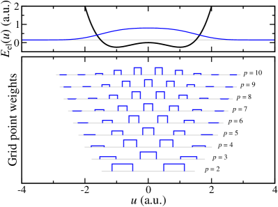
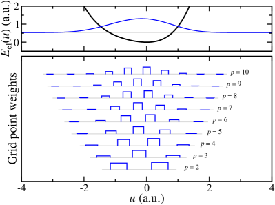
Larger grids can be constructed for any vibrational wave function by numerically solving Eq. 21. In Figs. 1 and 2 we show 2- to 10-point grids obtained for a symmetric and a non-symmetric anharmonic potential, respectively. The convergence of the grid weights to the square of the vibrational wave function can be appreciated in the plots.

Figure 1: Symmetric anharmonic potential $E_{\rm el}(u)=-\frac{1}{2}u^{2}+\frac{1}{4}u^{4}$ with its ground-state wave function (top panel), and quadrature grids constructed using this wave function (bottom panel).

Figure 2: Non-symmetric anharmonic potential $E_{\rm el}(u)=\frac{1}{2}u^{2}+\frac{1}{4}u^{3}+\frac{1}{8}u^{4}$ with its ground-state wave function (top panel), and quadrature grids constructed using this wave function (bottom panel).

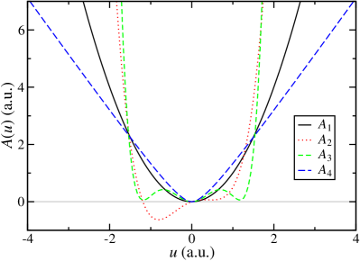
We test these numerical grids by integrating four test functions which can be regarded as models of the dependence of an electronic observable $A$ on the mode amplitude $u$. Our test functions are a pure quadratic function, $A_{1}=u^{2}$, a non-monotonic, non-symmetric quartic polynomial which takes negative values, $A_{2}=0.5u-u^{2}+u^{4}$, a non-monotonic, symmetric, non-negative sixth-order polynomial, $A_{3}=2u^{2}-2.8u^{4}+u^{6}$, and a monotonic, non-negative, non-polynomial function locally dominated by a quadratic term, $A_{4}=\frac{4u^{2}}{1+2|u|}$. These functions are plotted in Fig. 3. Functions similar to $A_{2}$ and $A_{3}$ have been used to model band gaps in some systems, Whalley_perovskites_2016 while functions with the linear asymptotic behavior of $A_{4}$ have been reported in previous studies. monserrat_giant_2015 ; antonius_anh_2015

Figure 3: Test functions $A_{1}=u^{2}$, $A_{2}=0.5u-u^{2}+u^{4}$, $A_{3}=2u^{2}-2.8u^{4}+u^{6}$, and $A_{4}=\frac{4u^{2}}{1+2|u|}$, which serve as models of the dependence of an electronic observable $A$ on mode amplitude $u$.

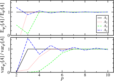
The convergence of the variance of $A$ is particularly relevant to the multi-dimensional Monte Carlo sampling of quadrature grids. By construction, the bias in any expectation value obtained with a $p$-point quadrature grid is ${\cal O}(u^{2p})$. Therefore, if $A$ is a polynomial of order $n_{A}$, its quadrature grid expectation value converges to the exact value at order $p=\lceil\frac{n_{A}+1}{2}\rceil$, while the variance of $A$ is a polynomial of order $2n_{A}$ and its quadrature grid estimate converges to the exact variance at $p=n_{A}+1$. Thus, if the variance approaches its exact value monotonically from below, it would be possible to obtain the exact expectation value of $A$ with a smaller uncertainty than with direct Monte Carlo by stochastically sampling a quadrature grid of $\lceil\frac{n_{A}+1}{2}\rceil\leq p<n_{A}+1$ points. Knowledge of $n_{A}$ for any given expectation value would then allow selecting the grid size $p=\lceil\frac{n_{A}+1}{2}\rceil$ that maximizes the efficiency of the stochastic sampling and incurs zero bias.

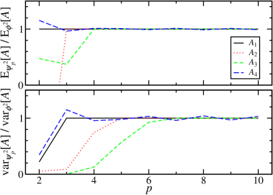
In Figs. 4 and 5 we plot the expectation value and variance of the four test functions for the symmetric and non-symmetric numerical grids, respectively. In these tests, the integrals of polynomials of order $n_{A}$ are approximated particularly poorly by grids with $p<\lceil\frac{n_{A}+1}{2}\rceil$ points. For $\lceil\frac{n_{A}+1}{2}\rceil\leq p<n_{A}+1$ the quadrature integrals are exact, as expected, while the variance approaches its exact value from below, making stochastic quadrature grid integration advantageous over direct Monte Carlo at these grid sizes.

The expectation value and variance of the non-polynomial $A_{4}$ test function converge slowly and non-monotonically to their respective exact values, but the quadrature integrals of $A_{4}$ are reasonably good approximations to the exact integral at all $p$, and two-point grids are particularly efficient since the corresponding variances are small (or indeed, zero for a symmetric wave function).

Figure 4: Quadrature-grid expectation value (top panel) and variance (bottom panel) of each of the four test functions plotted in Fig. 3 relative to the exact expectation value and variance, respectively, as a function of the number of points $p$ in the symmetric grids plotted in Fig. 1.

Figure 5: Quadrature-grid expectation value (top panel) and variance (bottom panel) of each of the four test functions plotted in Fig. 3 relative to the exact expectation value and variance, respectively, as a function of the number of points $p$ in the non-symmetric grids plotted in Fig. 2.

V $n$-dimensional Monte Carlo sampling of one-dimensional quadrature grids

We define quadrature grids for each of the $n$ normal-mode coordinates, which are stochastically sampled by choosing random grid points with probability proportional to their weights. The basic properties of expectation values of functions of $n$ variables differ from those in one dimension due to the effect of multi-mode contributions. As in the case of thermal lines, $n$-dimensional sampling of $p$-point quadrature grids correctly accounts for multi-mode contributions to the expectation value involving up to the $(2p-1)$th power of normal-mode coordinates, exceeding the order to which single-mode contributions are exact. Therefore we do not expect major differences in the behavior and convergence properties of $n$-dimensional quadrature grid expectation values with respect to the one-dimensional case.

Observables along most of the normal modes in a system are found in practice to be strongly quadratic, and therefore it is particularly interesting to investigate the use of per-mode grid sizes adapted to the specific system under consideration. We test $n$-dimensional sampling of quadrature grids by evaluating the zero-point correction to the band gap of a primitive cell of the HF and NH₃ molecular crystals using the harmonic vibrational wave function. These systems were found to be particularly problematic under the quadratic approximation in Ref. monserrat_giant_2015, , and therefore our results should be representative of the usefulness of multi-point quadrature grids in difficult cases. The band gap of HF is a markedly non-quadratic function of the highest-frequency normal mode, similar in shape to the one-dimensional test function $A_{4}$ in Section IV, see Fig. 2 of Ref. monserrat_giant_2015, , while it is found to be a strongly quadratic function of the 20 remaining normal modes. We similarly find that the non-quadratic behavior of the band gap of NH₃ arises largely from two mid-frequency normal modes, with the 43 remaining modes providing mostly quadratic contributions. This information allows us to choose which normal modes to sample using grids of $p>2$ points.

The local value of the band gap at each nuclear configuration is evaluated using the plane-wave DFT method with the PBE functional perdew_pbe_1996 as implemented in the castep code, clark_castep_2005 and vibrational calculations are performed using our own code. We use symmetrized sampling for all of our calculations, and we test (i) varying the number of grid points along all normal modes, and (ii) varying the number of grid points only along the modes for which we find the band gap to be non-quadratic, using two-point grids for the remaining modes.

Figure 6: (a) expectation value and (b) sample variance of the zero-point correction to the band gap of a primitive cell of the HF molecular crystal as a function of the grid size along all normal modes (black circles) and only along the mode for which the band gap is found to be non-quadratic, with the remaining modes using two-point grids (red diamonds). The horizontal blue lines represent the exact results evaluated by direct Monte Carlo integration, the light-colored areas represent their standard errors, and the horizontal green dotted line is the expectation value obtained with the quadratic approximation.

Figure 7: (a) expectation value and (b) sample variance of the zero-point correction to the band gap of a primitive cell of the NH₃ molecular crystal as a function of the grid size along all normal modes (black circles) and only along the two modes for which the band gap is found to be non-quadratic, with the remaining modes using two-point grids (red diamonds). The horizontal blue lines represent the exact results evaluated by direct Monte Carlo integration, the light-colored areas represent their standard errors, and the horizontal green dotted line is the expectation value obtained with the quadratic approximation.

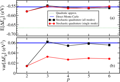
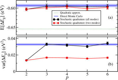
The expectation value and variance of the band gap of HF and NH₃ are plotted in Figs. 6 and 7, respectively, as a function of the number of points $p$ in the integration grid.

The results using $p$ grid points along all normal modes converge quickly towards the infinite grid limit. The sample variance is within statistical uncertainty of this limit for $p\geq 3$, implying that, while quadrature grids with $p>2$ offer excellent results for these systems, they offer no speed advantage over direct Monte Carlo integration. Only two-point grids (thermal lines) provide a significant reduction in statistical uncertainty, while still improving upon the quadratic approximation thanks to correctly accounting for multi-mode contributions.

In the case of the HF molecular crystal, limiting the use of grids with $p>2$ points to the normal mode of which the band gap is a non-quadratic function gives expectation values within statistical uncertainty of the direct Monte Carlo result, but with about half the sample variance. This implies a $\sim 30\%$ reduction in the number of samples needed to obtain the expectation value to a target statistical uncertainty. For NH₃ the uncertainty in the expectation value of the band gap prevents drawing strong conclusions regarding the selective application of multi-point grids, but the results hint at a reduced bias compared with $p=2$, and the sample variance is again about half that obtained with direct Monte Carlo.

These results reflect that, even when non-quadratic behavior is present in an observable, the overall weight of non-quadratic contributions to the result is typically small; two-point grids provide a very good approximation for quadratic contributions, and multi-point grids can be used along specific modes to avoid any bias.

VI Conclusions

We have quantified the bias incurred by the thermal lines method, which includes higher-order terms than the quadratic approximation, and we have reformulated thermal lines as a particular choice of grid size in a stochastic implementation of quadrature grid integration. We have demonstrated the construction of one-dimensional quadrature grids adapted to specific anharmonic wave functions and their application to the integration of functions modelling the dependence of electronic observables on nuclear configurations.

The accuracy of quadrature integration ultimately depends on the function being integrated. Our tests with model polynomials show that small grid sizes can incur a large bias, but knowledge of the order of the polynomial allows exploiting the slow convergence of the variance with grid size to obtain accurate expectation values with little statistical noise.

Our tests using DFT data indicate that observables of interest tend to be dominated by quadratic contributions, for which two-point grids (thermal lines) are ideally suited. However examples have been reported of observables with strong non-quadratic components along specific modes, monserrat_giant_2015 ; antonius_anh_2015 ; Whalley_perovskites_2016 and we find that selectively using quadrature grids with three or more points along these modes eliminates the bias in the expectation values.

We therefore recommend that the behavior of observables along each normal mode be determined prior to the application of stochastic quadrature grid integration in order to select the optimal grid size and avoid incurring a bias. This type of analysis can be trivially performed during the mapping of the Born-Oppenheimer energy surface $E_{\rm el}({\bf u})$ involved in solving anharmonic vibrational Hamiltonians, and can be carried out separately by direct inspection when using the harmonic approximation.