Beyond Sparsity: Tree Regularization of Deep Models for Interpretability

Abstract

The lack of interpretability remains a key barrier to the adoption of deep models in many applications. In this work, we explicitly regularize deep models so human users might step through the process behind their predictions in little time. Specifically, we train deep time-series models so their class-probability predictions have high accuracy while being closely modeled by decision trees with few nodes. Using intuitive toy examples as well as medical tasks for treating sepsis and HIV, we demonstrate that this new tree regularization yields models that are easier for humans to simulate than simpler L1 or L2 penalties without sacrificing predictive power.

1 Introduction

Deep models have become the de-facto approach for prediction in a variety of applications such as image classification (e.g. (?)) and machine translation (e.g. (?; ?)). However, many practitioners are reluctant to adopt deep models because their predictions are difficult to interpret. In this work, we seek a specific form of interpretability known as human-simulability. A human-simulatable model is one in which a human user can “take in input data together with the parameters of the model and in reasonable time step through every calculation required to produce a prediction” (?). For example, small decision trees with only a few nodes are easy for humans to simulate and thus understand and trust. In contrast, even simple deep models like multi-layer perceptrons with a few dozen units can have far too many parameters and connections for a human to easily step through. Deep models for sequences are even more challenging. Of course, decision trees with too many nodes are also hard to simulate. Our key research question is: can we create deep models that are well-approximated by compact, human-simulatable models?

The question of creating accurate yet human-simulatable models is an important one, because in many domains simulatability is paramount. For example, despite advances in deep learning for clinical decision support (e.g. (?; ?; ?)), the clinical community remains skeptical of machine learning systems (?). Simulatability allows clinicians to audit predictions easily. They can manually inspect changes to outputs under slightly-perturbed inputs, check substeps against their expert knowledge, and identify when predictions are made due to systemic bias in the data rather than real causes. Similar needs for simulatability exist in many decision-critical domains such as disaster response or recidivism prediction.

To address this need for interpretability, a number of works have been developed to assist in the interpretation of already-trained models. ? (?) train decision trees that mimic the predictions of a fixed, pretrained neural network, but do not train the network itself to be simpler. Other post-hoc interpretations typically typically evaluate the sensitivity of predictions to local perturbations of inputs or the input gradient (?; ?; ?; ?; ?). In parallel, research efforts have emphasized that simple lists of (perhaps locally) important features are not sufficient: ? (?) provide explanations in the form of programs; ? (?) learn decision sets and show benefits over other rule-based methods.

These techniques focus on understanding already learned models, rather than finding models that are more interpretable. However, it is well-known that deep models often have multiple optima of similar predictive accuracy (?), and thus one might hope to find more interpretable models with equal predictive accuracy. However, the field of optimizing deep models for interpretability remains nascent. ? (?) penalize input sensitivity to features marked as less relevant. ? (?) train deep models that make predictions from text and simultaneously highlight contiguous subsets of words, called a “rationale,” to justify each prediction. While both works optimize their deep models to expose relevant features, lists of features are not sufficient to simulate the prediction.

Contributions.

In this work, we take steps toward optimizing deep models for human-simulatability via a new model complexity penalty function we call tree regularization. Tree regularization favors models whose decision boundaries can be well-approximated by small decision-trees, thus penalizing models that would require many calculations to simulate predictions. We first demonstrate how this technique can be used to train simple multi-layer perceptrons to have tree-like decision boundaries. We then focus on time-series applications and show that gated recurrent unit (GRU) models trained with strong tree-regularization reach a high-accuracy-at-low-complexity sweet spot that is not possible with any strength of L1 or L2 regularization. Prediction quality can be further boosted by training new hybrid models – GRU-HMMs – which explain the residuals of interpretable discrete HMMs via tree-regularized GRUs. We further show that the approximate decision trees for our tree-regularized deep models are useful for human simulation and interpretability. We demonstrate our approach on a speech recognition task and two medical treatment prediction tasks for patients with sepsis in the intensive care unit (ICU) and for patients with human immunodeficiency virus (HIV). Throughout, we also show that standalone decision trees as a baseline are noticeably less accurate than our tree-regularized deep models. We have released an open-source Python toolbox to allow others to experiment with tree regularization .

Related work.

While there is little work (as mentioned above) on optimizing models for interpretability, there are some related threads. The first is model compression, which trains smaller models that perform similarly to large, black-box models (e.g. (?; ?; ?; ?)). Other efforts specifically train very sparse networks via L1 penalties (?) or even binary neural networks (?; ?) with the goal of faster computation. Edge and node regularization is commonly used to improve prediction accuracy (?; ?), and recently ? (?) improve prediction accuracy by training neural networks so that predictions match a small list of known domain-specific first-order logic rules. Sometimes, these regularizations—which all smooth or simplify decision boundaries—can have the effect of also improving interpretability. However, there is no guarantee that these regularizations will improve interpretability; we emphasize that specifically training deep models to have easily-simulatable decision boundaries is (to our knowledge) novel.

2 Background and Notation

We consider supervised learning tasks given datasets of $N$ labeled examples, where each example (indexed by $n$) has an input feature vectors $x_{n}$ and a target output vector $y_{n}$. We shall assume the targets $y_{n}$ are binary, though it is simple to extend to other types. When modeling time series, each example sequence $n$ contains $T_{n}$ timesteps indexed by $t$ which each have a feature vector $x_{nt}$ and an output $y_{nt}$. Formally, we write: $x_{n}=[x_{n1}\ldots x_{nT_{n}}]$ and $y_{n}=[y_{n1}\ldots y_{nT_{n}}]$. Each value $y_{nt}$ could be prediction about the next timestep (e.g. the character at time $t+1$) or some other task-related annotation (e.g. if the patient became septic at time $t$).

Simple neural networks.

A multi-layer perceptron (MLP) makes predictions $\hat{y}_{n}$ of the target $y_{n}$ via a function $\hat{y}_{n}(x_{n},W)$, where the vector $W$ represents all parameters of the network. Given a data set $\{(x_{n},y_{n})\}$, our goal is to learn the parameters $W$ to minimize the objective

$$\min_{W}\lambda\Psi(W)+\sum_{n=1}^{N}\mbox{loss}(y_{n},\hat{y}_{n}(x_{n},W))$$ (1)

For binary targets $y_{n}$, the logistic loss (binary cross entropy) is an effective choice. The regularization term $\Psi(W)$ can represent L1 or L2 penalties (e.g. (?; ?; ?)) or our new regularization.

Recurrent Neural Networks with Gated Recurrent Units.

A recurrent neural network (RNN) takes as input an arbitrary length sequence $x_{n}=[x_{n1}\ldots x_{nT_{n}}]$ and produces a “hidden state” sequence $h_{n}=[h_{n1}\ldots h_{nT_{n}}]$ of the same length as the input. Each hidden state vector at timestep $t$ represents a location in a (possibly low-dimensional) “state space” with $K$ dimensions: $h_{nt}\in\mathbb{R}^{K}$. RNNs perform sequential nonlinear embedding of the form $h_{nt}=f(x_{nt},h_{nt-1})$ in hope that the state space location $h_{nt}$ is a useful summary statistic for making predictions of the target $y_{nt}$ at timestep $t$.

Many different variants of the transition function architecture $f$ have been proposed to solve the challenge of capturing long-term dependencies. In this paper, we use gated recurrent units (GRUs) (?), which are simpler than other alternatives such as long short-term memory units (LSTMs) (?). While GRUs are convenient, any differentiable RNN architecture is compatible with our new tree-regularization approach.

Below we describe the evolution of a single GRU sequence, dropping the sequence index $n$ for readability. The GRU transition function $f$ produces the state vector $h_{t}=[h_{t1}\ldots h_{tK}]$ from a previous state $h_{t-1}$ and an input vector $x_{t}$, via the following feed-forward architecture:

$$\textup{output state}:h_{tk} =(1-z_{tk})h_{t-1,k}+z_{t,k}\tilde{h}_{tk}$$ (2)

$$\textup{candidate state}:\tilde{h}_{tk} =\textup{tanh}(V_{k}^{h}x_{t}+U_{k}^{h}(r_{t}\odot h_{t-1}))$$

$$\textup{update gate}:z_{tk} =\sigma(V_{k}^{z}x_{t}+U_{k}^{z}h_{t-1})$$

$$\textup{reset gate}:r_{tk} =\sigma(V_{k}^{r}x_{t}+U_{k}^{r}h_{t-1})$$

The internal network nodes include candidate state gates $\tilde{h}$, update gates $z$ and reset gates $r$ which have the same cardinalty as the state vector $h$. Reset gates allow the network to forget past state vectors when set near zero via the logistic sigmoid nonlinearity $\sigma(\cdot)$. Update gates allow the network to either pass along the previous state vector unchanged or use the new candidate state vector instead. This architecture is diagrammed in Figure 1.

Figure 1: Diagram of gated recurrent unit (GRU) used for each timestep our neural time-series model. The orange triangle indicates the predicted output $\hat{y}_{t}$ at time $t$.

The predicted probability of the binary label $y_{t}$ for time $t$ is a sigmoid transformation of the state at time $t$:

$$\hat{y}_{t}=\sigma(w^{T}h_{t})$$ (3)

Here, weight vector $w\in\mathbb{R}^{K}$ represents the parameters of this output layer. We denote the parameters for the entire GRU-RNN model as $W=(w,U,V)$, concatenating all component parameters. We can train GRU-RNN time-series models (hereafter often just called GRUs) via the following loss minimization objective:

$$\min_{W}\lambda\Psi(W)+\sum_{n=1}^{N}\sum_{n=1}^{T_{n}}\mbox{loss}(y_{nt},\hat{y}_{nt}(x_{n},W))$$ (4)

where again $\Psi(W)$ defines a regularization cost.

3 Tree Regularization for Deep Models

We now propose a novel tree regularization function $\Omega(W)$ for the parameters of a differentiable model which attempts to penalize models whose predictions are not easily simulatable. Of course, it is difficult to measure “simulatability” directly for an arbitrary network, so we take inspiration from decision trees. Our chosen method has two stages: first, find a single binary decision tree which accurately reproduces the network’s thresholded binary predictions $\hat{y}_{n}$ given input $x_{n}$. Second, measure the complexity of this decision tree as the output of $\Omega(W)$. We measure complexity as the average decision path length—the average number of decision nodes that must be touched to make a prediction for an input example $x_{n}$. We compute the average with respect to some designated reference dataset of example inputs $D=\{x_{n}\}$ from the training set. While many ways to measure complexity exist, we find average path length is most relevant to our notion of simulatability. Remember that for us, human simulation requires stepping through every calculation required to make a prediction. Average path length exactly counts the number of true-or-false boolean calculations needed to make an average prediction, assuming the model is a decision tree. Total number of nodes could be used as a metric, but might penalize more accurate trees that have short paths for most examples but need more involved logic for few outliers.

Our true-average-path-length cost function $\Omega(W)$ is detailed in Alg. 1. It requires two subroutines, TrainTree and PathLength. TrainTree trains a binary decision tree to accurately reproduce the provided labeled examples $\{x_{n},\hat{y}_{n}\}$. We use the DecisionTree module distributed in Python’s scikit-learn (?) with post-pruning to simplify the tree. These trees can give probabilistic predictions at each leaf. (Complete decision-tree training details are in the supplement.) Next, PathLength counts how many nodes are needed to make a specific input to an output node in the provided decision tree. In our evaluations, we will apply our average-decision-tree-path-length regularization, or simply “tree regularization,” to several neural models.

Algorithm 1 Average-Path-Length Cost Function

1:

2:$\hat{y}(\cdot,W)$ : binary prediction function, with parameters $W$

3:$D=\{x_{n}\}_{n=1}^{N}$ : reference dataset with $N$ examples

4:function $\Omega$($W$)

5:     $\mbox{tree}\leftarrow\textsc{TrainTree}(\{x_{n},\hat{y}(x_{n},W)\})$

6:     return $\frac{1}{N}\sum_{n}\textsc{PathLength}(\mbox{tree},x_{n})$

Alg. 1 defines our average-path-length cost function $\Omega(W)$, which can be plugged into the abstract regularization term $\Psi(W)$ in the objectives in equations 1 and 4.

Making the Decision-Tree Loss Differentiable

Training decision trees is not differentiable, and thus $\Omega(W)$ as defined in Alg. 1 is not differentiable with respect to the network parameters $W$ (unlike standard regularizers such as the L1 or L2 norm). While one could resort to derivative-free optimization techniques (?), gradient descent has been an extremely fast and robust way of training networks (?).

A key technical contribution of our work is introducing and training a surrogate regularization function $\hat{\Omega}(W):\mbox{supp}(W)\rightarrow\mathbb{R}_{+}$ to map each candidate neural model parameter vector $W$ to an estimate of the average-path-length. Our approximate function $\hat{\Omega}$ is implemented as a standalone multi-layer perceptron network and is thus differentiable. Let vector $\xi$ of size $k$ denote the parameters of this chosen MLP approximator. We can train $\hat{\Omega}$ to be a good estimator by minimizing a squared error loss function:

$$\min_{\xi}\textstyle\sum_{j=1}^{J}(\Omega(W_{j})-\hat{\Omega}(W_{j},\xi))^{2}+\epsilon||\xi||_{2}^{2}$$ (5)

where $W_{j}$ are the entire set of parameters for our model, $\epsilon>0$ is a regularization strength, and we assume we have a dataset of $J$ known parameter vectors and their associated true path-lengths: $\{W_{j},\Omega(W_{j})\}_{j=1}^{J}$. This dataset can be assembled using the candidate $W$ vectors obtained while training our target neural model $\hat{y}(\cdot,W)$, as well as by evaluating $\Omega(W)$ for randomly generated $W$. Importantly, one can train the surrogate function $\hat{\Omega}$ in parallel with our network. In the supplement, we show evidence that our surrogate predictor $\hat{\Omega}(\cdot)$ tracks the true average path length as we train the target predictor $\hat{y}(\cdot,W)$.

Training the Surrogate Loss

Even moderately-sized GRUs can have parameter vectors $W$ with thousands of dimensions. Our labeled dataset for surrogate training – $\{W_{j},\Omega(W_{j})\}_{j=1}^{J}$—will only have one $W_{j}$ example from each target network training iteration. Thus, in early iterations, we will have only few examples from which to learn a good surrogate function $\hat{\Omega}(W)$. We resolve this challenge via augmenting our training set with additional examples: We randomly sample weight vectors $W$ and calculate the true average path length $\Omega(W)$, and we also perform several random restarts on the unregularized GRU and use those weights in our training set.

A second challenge occurs later in training: as the model parameters $W$ shift away from their initial values, those early parameters may not be as relevant in characterizing the current decision function of the GRU. To address this, for each epoch, we use examples only from the past $E$ epochs (in addition to augmentation), where in practice, $E$ is empirically chosen. Using examples from a fixed window of epochs also speeds up training. The supplement shows a comparison of the importance of these heuristics for efficient and accurate training—empirically, data augmentation for stabilizing surrogate training allows us to scale to GRUs with 100s of nodes. GRUs of this size are sufficient for many real problems, such as those we encounter in healthcare domains.

Typically, we use $J=50$ labeled pairs for surrogate training for toy datasets and $J=100$ for real world datasets. Optimization of our surrogate objective is done via gradient descent. We use Autograd to compute gradients of the loss in Eq. (5) with respect to $\xi$, then use Adam to compute descent directions with step sizes set to 0.01 for toy datasets and 0.001 for real world datasets.

4 Tree-Regularized MLPs: A Demonstration

While time-series models are the main focus of this work, we first demonstrate tree regularization on a simple binary classification task to build intuition. We call this task the 2D Parabola problem, because as Fig. 2(a) shows, the training data consists of 2D input points whose two-class decision boundary is roughly shaped like a parabola. The true decision function is defined by $y=5*(x-0.5)^{2}+0.4$. We sampled 500 input points $x_{n}$ uniformly within the unit square $[0,1]\times[0,1]$ and labeled those above the decision function as positive. To make it easy for models to overfit, we flipped 10% of the points in a region near the boundary. A random 30% were held out for testing.

For the classifier $\hat{y}$, we train a 3-layer MLP with 100 first layer nodes, 100 second layer nodes, and 10 third layer nodes. This MLP is intentionally overly expressive to encourage overfitting and expose the impact of different forms of regularization: our proposed tree regularization $\Psi(W)=\hat{\Omega}(W)$ and two baselines: an L2 penalty on the weights $\Psi(W)=||W||_{2}$, and an L1 penalty on the weights $\Psi(W)=||W||_{1}$. For each regularization function, we train models at many different regularization strengths $\lambda$ chosen to explore the full range of decision boundary complexities possible under each technique.

For our tree regularization, we model our surrogate $\hat{\Omega}(W)$ with a 1-hidden layer MLP with 25 units. We find this simple architecture works well, but certainly more complex MLPs could could be used on more complex problems. The objective in equation 1 was optimized via Adam gradient descent (?) using a batch size of 100 and a learning rate of 1e-3 for 250 epochs, and hyperparameters were set via cross validation using grid search (see supplement for full experimental details).

Fig. 2 (b) shows the each trained model as a single point in a 2D fitness space: the x-axis measures model complexity via our average-path-length metric, and the y-axis measures AUC prediction performance. These results show that simple L1 or L2 regularization does not produce models with both small node count and good predictions at any value of the regularization strength $\lambda$. As expected, large $\lambda$ values for L1 and L2 only produce far-too-simple linear decision boundaries with poor accuracies. In contrast, our proposed tree regularization directly optimizes the MLP to have simple tree-like boundaries at high $\lambda$ values which can still yield good predictions.

The lower panes of Fig. 2 shows these boundaries. Our tree regularization is uniquely able to create axis-aligned functions, because decision trees prefer functions that are axis-aligned splits. These axis-aligned functions require very few nodes but are more effective than L1 and L2 counterparts. The L1 boundary is more sharp, whereas the L2 is more round.

(a) Training Data and Binary Class Labels for 2D Parabola

(b) Prediction quality and complexity as reg. strength $\lambda$ varies

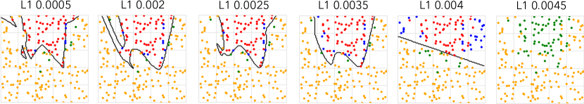
(c) Decision Boundaries with L1 regularization

(d) Decision Boundaries with L2 regularization

(e) Decision Boundaries Tree regularization

Figure 2: 2D Parabola task: (a) Each training data point in 2D space, overlaid with true parabolic class boundary. (b): Each method’s prediction quality (AUC) and complexity (path length) metrics, across range of regularization strength $\lambda$. In the small path length regime between 0 and 5, tree regularization produces models with higher AUC than L1 or L2. (c-e): Decision boundaries (black lines) have qualitatively different shapes for different regularization schemes, as regularization strength $\lambda$ increases. We color predictions as true positive (red), true negative (yellow), false negative (green), and false positive (blue).

5 Tree-Regularized Time-Series Models

We now evaluate our tree-regularization approach on time-series models. We focus on GRU-RNN models, with some later experiments on new hybrid GRU-HMM models. As with the MLP, each regularization technique (tree, L2, L1) can be applied to the output node of the GRU across a range of strength parameters $\lambda$. Importantly, Algorithm  1 can compute the average-decision-tree-path-length for any fixed deep model given its parameters, and can hence be used to measure decision boundary complexity under any regularization, including L1 or L2. This means that when training any model, we can track both the predictive performance (as measured by area-under-the-ROC-curve (AUC); higher values mean better predictions), as well as the complexity of the decision tree required to explain each model (as measured by our average path length metric; lower values mean more interpretable models). We also show results for a baseline standalone decision tree classifier without any associated deep model, sweeping a range of parameters controlling leaf size to explore how this baseline trades off path length and prediction quality. Further details of our experimental protocol are in the supplement, as well as more extensive results with additional baselines.

5.1 Tasks

Synthetic Task: Signal-and-noise HMM

We generated a toy dataset of $N=100$ sequences, each with $T=50$ timesteps. Each timestep has a data vector $x_{nt}$ of 14 binary features and a single binary output label $y_{nt}$. The data comes from two separate HMM processes. First, a “signal” HMM generates the first 7 data dimensions from 5 well-separated states. Second, an independent “noise” HMM generates the remaining 7 data dimensions from a different set of 5 states. Each timestep’s output label $y_{nt}$ is produced by a rule involving both the signal data and the signal hidden state: the target is 1 at timestep $t$ only if both the first signal state is active and the first observation is turned on. We deliberately designed the generation process so that neither logistic regression with $x$ as features nor an RNN model that makes predictions from hidden states alone can perfectly separate this data.

(a) GRU $\lambda=1$

(b) GRU $\lambda=800$

(c) GRU $\lambda=1\,000$

(d) GRU

Figure 3: Toy Signal-and-Noise HMM Task: (a)-(c) Decision trees trained to mimic predictions of GRU models with 25 hidden states at different regularization strengths $\lambda$; as expected, increasing $\lambda$ decreases the size of the learned trees (see supplement for more trees). Decision tree (c) suggests the model learns to predict positive output (blue) if and only if “x[0] == 1 and x[3] == 1 and x[4] == 0”, which is consistent with the true rule we used to generate labels: assign positive label only if first dimension is on (x[0] == 1) and first state is active (emission probabilities for this state: [.5 .5 .5 .5 0 $\ldots$]). (d) Tree-regularized GRU models reach a sweet spot of small path lengths yet high AUC predictions that alternatives cannot reach at any tested value of $\lambda$.

Real-World Tasks:

We tested our approach on several real tasks: predicting medical outcomes of hospitalized septic patients, predicting HIV therapy outcomes, and identifying stop phonemes in English speech recordings. To normalize scales, we independently standardized features $x$ via z-scoring.

• Sepsis Critical Care: We study time-series data for 11 786 septic ICU patients from the public MIMIC III dataset (?). We observe at each hour $t$ a data vector $x_{nt}$ of 35 vital signs and lab results as well as a label vector $y_{nt}$ of 5 binary outcomes. Hourly data $x_{nt}$ measures continuous features such as respiration rate (RR), blood oxygen levels (paO₂), fluid levels, and more. Hourly binary labels $y_{nt}$ include whether the patient died in hospital and if mechanical ventilation was applied. Models are trained to predict all 5 output dimensions concurrently from one shared embedding. The average sequence length is 15 hours. 7 070 patients are used in training, 1 769 for validation, and 294 for test.

  

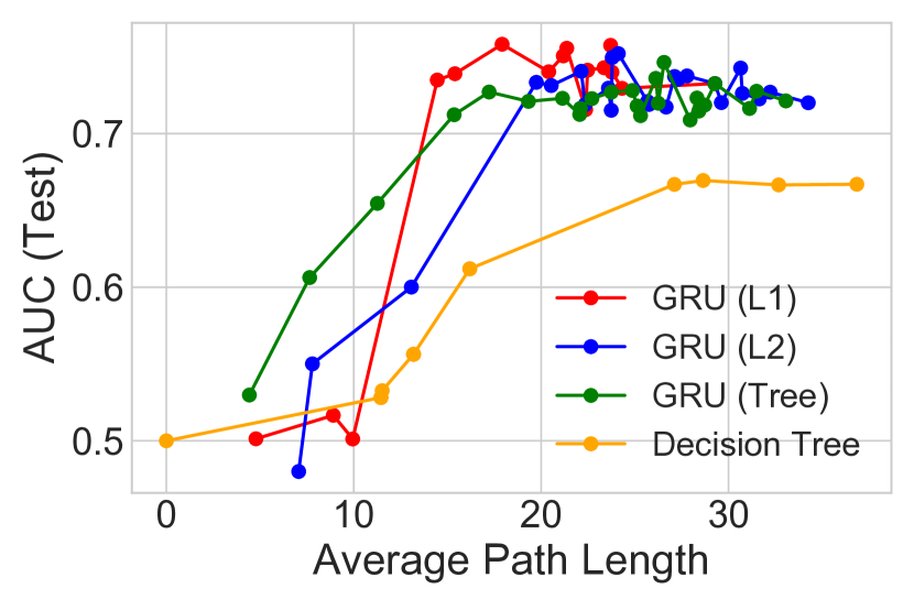
  (a) In-Hospital Mortality

  

  (b) In-Hospital Mortality

  

  (c) Mechanical Ventilation

  

  (d) Mechanical Ventilation

  Figure 4: Sepsis task: Study of different regularization techniques for GRU model with 100 states, trained to jointly predict 5 binary outcomes. Panels (a) and (c) show AUC vs. average path length for 2 of the 5 outcomes (remainder in the supplement); in both cases, tree-regularization provides higher accuracy in the target regime of low-complexity decision trees. Panels (b) and (d) show the associated decision trees for $\lambda=2\,000$; these were found by clinically interpretable by an ICU clinician (see main text).

• HIV Therapy Outcome (HIV): We use the EuResist Integrated Database (?) for 53 236 patients diagnosed with HIV. We consider 4-6 month intervals (corresponding to hospital visits) as time steps. Each data vector $x_{nt}$ has 40 features, including blood counts, viral load measurements and lab results. Each output vector $y_{nt}$ has 15 binary labels, including whether a therapy was successful in reducing viral load to below detection limits, if therapy caused CD4 blood cell counts to drop to dangerous levels (indicating AIDS), or if the patient suffered adherence issues to medication. The average sequence length is 14 steps. 37 618 patients are used for training; 7 986 for testing, and 7 632 for validation.

• Phonetic Speech (TIMIT): We have recordings of 630 speakers of eight major dialects of American English reading ten phonetically rich sentences (?). Each sentence contains time-aligned transcriptions of 60 phonemes. We focus on distinguishing stop phonemes (those that stop the flow of air, such as “b” or “g”) from non-stops. Each timestep has one binary label $y_{nt}$ indicating if a stop phoneme occurs or not. Each input $x_{nt}$ has 26 continuous features: the acoustic signal’s Mel-frequency cepstral coefficients and derivatives. There are 6 303 sequences, split into 3 697 for training, 925 for validation, and 1 681 for testing. The average length is 614.

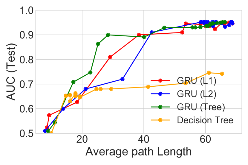
(a) TIMIT Stop Phonemes

(b) HIV: CD4⁺ $\leq$ 200 cells/ml

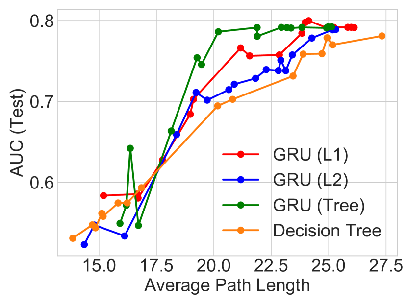
(c) HIV Therapy Adherence

(d) HIV Therapy Adherence

Figure 5: TIMIT and HIV tasks: Study of different regularization techniques for GRU model with 75 states. Panels (a)-(c) are tradeoff curves showing how AUC predictive power and decision-tree complexity evolve with increasing regularization strength under L1, L2 or tree regularization on both TIMIT and HIV tasks. The GRU is trained to jointly predict 15 binary outcomes for HIV, of which 2 are shown here in Panels (b) - (c). The GRU’s decision tree proxy for HIV Adherence is shown in (d).

5.2 Results

The major conclusions of our experiments comparing GRUs with various regularizations are outlined below.

Tree-regularized models have fewer nodes than other forms of regularization.

Across tasks, we see that in the target regime of small decision trees (low average-path lengths), our proposed tree-regularization achieves higher prediction quality (higher AUCs). In the signal-and-noise HMM task, tree regularization (green line in Fig. 3(d)) achieves AUC values near 0.9 when its trees have an average path length of 10. Similar models with L1 or L2 regularization reach this AUC only with trees that are nearly double in complexity (path length over 25). On the Sepsis task (Fig. 4) we see AUC gains of 0.05-0.1 at path lengths of 2-10. On the TIMIT task (Fig. 5(a)), we see AUC gains of 0.05-0.1 at path lengths of 20-30. Finally, on the HIV CD4 blood cell count task in Fig. 5(b), we see AUC differences of between 0.03 and 0.15 for path lengths of 10-15. The HIV adherence task in Fig. 5(d) has AUC gains of between 0.03 and 0.05 in the path length range of 19 to 25 while at smaller paths all methods are quite poor, indicating the problem’s difficulty. Overall, these AUC gains are particularly useful in determining how to administer subsequent HIV therapies.

We emphasize that our tree-regularization usually achieves a sweet spot of high AUCs at short path lengths not possible with standalone decision trees (orange lines), L1-regularized deep models (red lines) or L2-regularized deep models (blue lines). In unshown experiments, we also tested elastic net regularization (?), a linear combination of L1 and L2 penalities. We found elastic nets to follow the same trend lines as L1 and L2, with no visible differences. In domains where human-simulatability is required, increases in prediction accuracy in the small-complexity regime can mean the difference between models that provide value on a task and models that are unusable, either because performance is too poor or predictions are uninterpretable.

Our learned decision tree proxies are interpretable.

Across all tasks, the decision trees which mimic the predictions of tree-regularized deep models are small enough to simulate by hand (path length $\leq 25$) and help users grasp the model’s nonlinear prediction logic. Intuitively, the trees for our synthetic task in Fig. 3(a)-(c) decrease in size as the strength $\lambda$ increases. The logic of these trees also matches the true labeling process: even the simplest tree (c) checks a relevant subset of input dimensions necessary to verify that both the first state and the first output dimension are active.

In Fig. 4, we show decision tree proxies for our deep models on two sepsis prediction tasks: mortality and need for ventilation. We consulted a clinical expert on sepsis treatment, who noted that the trees helped him understand what the models might be doing and thus determine if he would trust the deep model. For example, he said that using FiO₂, RR, CO₂ and paO₂ to predict need for mechanical ventilation (Fig. 4(d)) was sensible, as these all measure breathing quality. In contrast, the in-hospital mortality tree (Fig. 4(b)) predicts that some young patients with no organ failure have high mortality rates while other young patients with organ failure have low mortality. These counter-intuitive results led to hypotheses about how uncaptured variables impact the training process. Such reasoning would not be possible from simple sensitivity analyses of the deep model.

Finally, we have verified that the decision tree proxies of our tree-regularized deep models of the HIV task in Fig. 5(d) are interpretable for understanding why a patient has trouble adhering to a prescription; that is, taking drugs regularly as directed. Our clinical collaborators confirm that the baseline viral load and number of prior treatment lines, which are prominent attributes for the decisions in Fig. 5(d), are useful predictors of a patient with adherence issues. Several medical studies (?; ?) suggest that patients with higher baseline viral loads tend to have faster disease progression, and hence have to take several drug cocktails to combat resistance. Juggling many drugs typically makes it difficult for these patients to adhere as directed. We hope interpretable predictive models for adherence could help assess a patient’s overall prognosis (?) and offer opportunities for intervention (e.g. with alternative single-tablet regimens).

Decision trees trained to mimic deep models make faithful predictions.

Across datasets, we find that each tree-regularized deep time-series model has predictions that agree with its corresponding decision tree proxy in about 85-90% of test examples. Table 1 shows exact fidelty scores for each dataset. Thus, the simulatable paths of the decision tree will be trustworthy in a majority of cases.

Practical runtimes for tree regularization are less than twice that of simpler L2.

While our tree-regularized GRU with 10 states takes 3977 seconds per epoch on TIMIT, a similar L2-regularized GRU takes 2116 seconds per epoch. Thus, our new method has cost less than twice the baseline even when the surrogate is serially computed. Because the surrogate $\hat{\Omega}(W)$ will in general be a much smaller model than the predictor $\hat{y}(x,W)$, we expect one could get faster per-epoch times by parallelizing the creation of $(W,\Omega(W))$ training pairs and the training of the surrogate $\hat{\Omega}(W)$. Additionally, 3977 seconds includes the time needed to train the surrogate. In practice, we do this sparingly, only once every 25 epochs, yielding an amortized per-epoch cost of 2191 seconds (more runtime results are in the supplement).

Decision trees are stable over multiple optimization runs.

When tree regularization is strong (high $\lambda$), the decision trees trained to match the predictions of deep models are stable. For both signal-and-noise and sepsis tasks, multiple runs from different random restarts have nearly identical tree shape and size, perhaps differing by a few nodes. This stability is crucial to building trust in our method. On the signal-and-noise task ($\lambda=7000$), 7 of 10 independent runs with random initializations resulted in trees of exactly the same structure, and the others closely resembled those sharing the same subtrees and features (more details in supplement).

Dataset	Fidelity
signal-and-noise HMM	0.88
SEPSIS (In-Hospital Mortality)	0.81
SEPSIS (90-Day Mortality)	0.88
SEPSIS (Mech. Vent.)	0.90
SEPSIS (Median Vaso.)	0.92
SEPSIS (Max Vaso.)	0.93
HIV (CD4+ below 200)	0.84
HIV (Therapy Success)	0.88
HIV (Mortality)	0.93
HIV (Poor Adherence)	0.90
HIV (AIDS Onset)	0.93
TIMIT	0.85

Table 1: Fidelity of predictions from our trained deep GRU-RNN and its corresponding decision tree. Fidelity is defined as the percentage of test examples on which the prediction made by a tree agrees with the deep model (?). We used 20 hidden GRU states for signal-and-noise task, 50 states for all others.

The deep residual GRU-HMM achieves high AUC with less complexity.

So far, we have focused on regularizing standard deep models, such as MLPs or GRUs. Another option is to use a deep model as a residual on another model that is already interpretable: for example, discrete HMMs partition timesteps into clusters, each of which can be inspected, but its predictions might have limited accuracy. In Fig. 6, we show the performance of jointly training a GRU-HMM, a new model which combines an HMM with a tree-regularized GRU to improve its predictions (details and further results in the supplement). Here, the ideal path length is zero, indicating only the HMM makes predictions. For small average-path-lengths, the GRU-HMM improves the original HMM’s predictions and has simulatability gains over earlier GRUs. On the mechanical ventilation task, the GRU-HMM requires an average path length of only 28 to reach AUC of 0.88, while the GRU alone with the same number of states requires a path length of 60 to reach the same AUC. This suggests that jointly-trained deep residual models may provide even better interpretability.

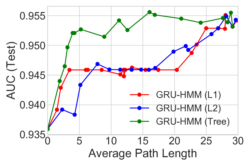
(a) Signal-and-noise 20+5

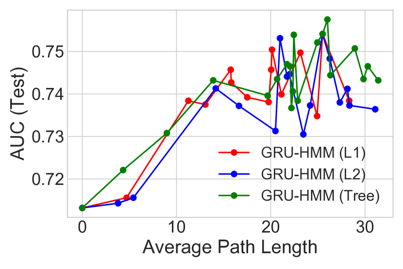
(b) In-Hosp. Mort. 50+50

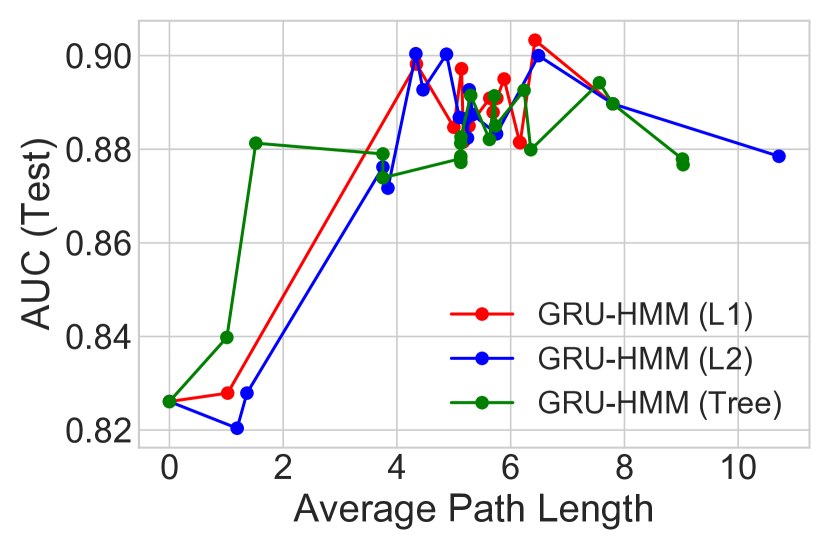
(c) Mech. Vent. 50+50

(d) Stop Phonemes 50+25

Figure 6: Fitness curves for the GRU-HMM, showing prediction quality (AUC) vs. complexity (path length) across range of regularization strengths $\lambda$. Captions show the number of HMM states plus the number of GRU states. See earlier figures to compare these GRU-HMM numbers to simpler GRU and decision tree baselines.

6 Discussion and Conclusion

We have introduced a novel tree-regularization technique that encourages the complex decision boundaries of any differentiable model to be well-approximated by human-simulatable functions, allowing domain experts to quickly understand and approximately compute what the more complex model is doing. Overall, our training procedure is robust and efficient; future work could continue to explore and increase the stability of the learned models as well as identify ways to apply our approach to situations in which the inputs are not inherently interpretable (e.g. pixels in an image).

Across three complex, real-world domains – HIV treatment, sepsis treatment, and human speech processing – our tree-regularized models provide gains in prediction accuracy in the regime of simpler, approximately human-simulatable models. Future work could apply tree regularization to local, example-specific approximations of a loss (?) or to representation learning tasks (encouraging embeddings with simple boundaries). More broadly, our general training procedure could apply tree-regularization or other procedure-regularization to a wide class of popular models, helping us move beyond sparsity toward models humans can easily simulate and thus trust.

Supplementary Material

Appendix A Details for Decision-Tree Training

Training decision trees with post-pruning.

Our average path length function $\Omega(W)$ for determining the complexity of a deep model with parameters $W$ – defined in the main paper in Alg. 1 – assumes that we have a robust, black-box way to train binary decision-trees called TrainTree given a labeled dataset $\{x_{n},\hat{y}_{n}\}$. For this we use the DecisionTree module distributed in Python’s sci-kit learn, which optimizes information gain with Gini impurity. The specific syntax we use (for reproducibility) is:

tree = DecisionTree(min_sample_count=5)
tree.fit(x_train, y_train)
tree = prune_tree(tree, x_valid, y_valid)

The provided keyword options force the tree to have at least 5 examples from the training set in every leaf. We found that tuning hyperparameters of the TrainTree subprocedure, such as the minimum size of a leaf node, to be important for making useful trees.

Generally, the runtime cost of sklearn’s fitting procedure scales superlinearly with the number of examples $N$ and linearly with the number of features $F$ – a total complexity of $O(FN\log(N))$. In practice, we found that with $N=1000$ examples, $F=10$ features, tree construction takes 15.3 microseconds.

The pruning procedure is a heuristic to create simpler trees, summarized in algorithm 2. After TrainTree delivers a working decision tree, we iterative propose removing each remaining leaf node, accepting the proposal if the squared prediction error on a validation set improves. This pruning removes sub-trees that don’t generalize to unseen data.

Algorithm 2 Post-pruning for training decision trees.

1:

2:$T$ : initial decision tree

3:$\textsc{ErrOnVal}(\cdot)$ : squared error on validation data

4:$\qquad\textsc{ErrOnVal}(T)\triangleq\sum_{n=1}^{N}(T(x_{n})-y_{n})^{2}$

5:procedure PruneTree( $T$, $err$ )

6:     $e\leftarrow\textsc{ErrOnVal}(T)$.

7:     for node $n\in\textsc{SortLeafToRoot}(T.nodes)$ do

8:         $T^{\prime}\leftarrow\textsc{RemoveNode}(T,n)$

9:         $e_{new}\leftarrow\textsc{ErrOnVal}(T^{\prime})$

10:         if $e_{new}<e$ then $T\leftarrow T^{\prime}$               

11:     Return $T$

Sanity check: Surrogate path length closely follow true path length.

Fig. A.1 shows that our surrogate predictor $\hat{\Omega}(\cdot)$ tracks the true average path length as we train the target predictor $\hat{y}(\cdot,W)$ on several different datasets.

(a) Path length estimates $\hat{\Omega}$ for 2D Parabola task

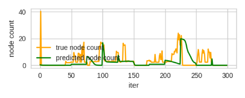
(b) Path length estimates $\hat{\Omega}$ for Signal-and-noise HMM task

Figure A.1: True average path lengths (yellow) and surrogate estimates $\hat{\Omega}$ (green) across many iterations of network parameter training iterations.

Sensitivity to different choices for surrogate training.

In Fig. A.2, we show sample learning curves for variations of methods for approximating the average path length (also called “node count”) in a decision tree. In blue is the true value. Each of the other 3 lines use the same surrogate model: an MLP with 25 hidden nodes. Increasing its capacity too much, i.e. 100 hidden nodes, leads to overfitting where the surrogate is able to predict the average path length extremely well for a small number of iterations, while the performance quickly decays. With an MLP of the right capacity, four additional tricks: (1) weight augmentation, (2) random restarts with an unregularized model, (3) fixed window of data, and (4) surrogate retraining greatly improve the accuracy of the average path length predictions.

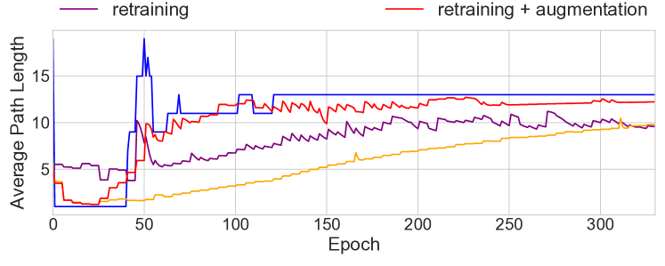
Figure A.2: This figure shows the effects of weight augmentation and retraining. The blue line is the true average path length of the decision tree at each epoch. All other lines show predicted path lengths using the surrogate MLP. By randomly sampling weights and intermittently retraining the surrogate, we significantly improve the ability of the surrogate model to track the changes in the ground truth.

Normally, if our differentiable model is a GRU, we compile examples using the GRU weights at every batch and calculate the true average path length. This dataset is used to train the surrogate model. If examples are very sparse, surrogate predictions may be unstable. Augmentation addresses this by randomly sampling weight vectors and computing the average path length to artificially create a larger dataset. Early epochs are especially problematic when it comes to lacking data. In addition to augmentation, we use random restarts to separately train unregularized GRUs (each with different weight initializations) to grow a dataset of weight vectors prior to training the regularized model.

As the GRU parameters take steps away from their initial values, our examples from those early epochs no longer describe the current state of the model. Retraining and a fixed window of data address this by re-learning the surrogate function at a fixed frequency using examples only from the last $J$ epochs. In practice, both the augmentation size, the retraining frequency, and $J$ are functions of the learning rate and the dataset size. See table B.1 for exact numbers.

Appendix B Experimental Protocol

See table B.1 for model hyperparameters for each dataset. For standard recurrent models such as HMM or GRU, the decision trees were trained on the input data and the predictions of the model’s output node. For our deep residual GRU-HMM, the decision trees were trained on the predictions on the GRU’s output node only. For both synthetic and real-world datasets, our surrogate to the tree loss is a multilayer perceptron with 1 hidden layer of 25 nodes. For each dataset, when we investigated several regularization strengths ($\lambda$), we initialize the model weights using the same random seed. We use the Adam algorithm (?) for all optimization.

Dataset	Total Num. Sequences	Avg. seq. length	Learning Rate	Batch size	Minimum Leaf Sample	Post-pruned	Epochs (Model)	Epochs (Surrogate)	Retraining Freq.	$J$
parabola	n/a	n/a	1e-2	32	0	N	250	500	100	n/a
signal-and-noise HMM	100	50	1e-2	10	25	Y	300	1000	50	50
HIV	53 236	14	1e-3	256	1 000	Y	300	5000	25	100
SEPSIS	11 786	15	1e-3	256	1 000	Y	300	5000	25	100
TIMIT	6 303	614	1e-3	256	5 000	Y	200	5000	25	100

Table B.1: Dataset summaries and training parameters used in our experiments.

B.1 2D Parabola

Dataset generation.

The training data consists of 2D input points whose two-class decision boundary is roughly shaped like a parabola. The true decision function is defined by $y=5*(x-0.5)^{2}+0.4$. We sampled all 200 input points $x_{n}$ uniformly within the unit square $[0,1]\times[0,1]$ and labeled those above the decision function as positive. To add randomness, we flipped 10% of the points in the region near the boundary between $y=5*(x-0.5)^{2}+0.2$ and $y=5*(x-0.5)^{2}+0.6$.

Regularization strengths.

Tested values of regularization strength parameter $\lambda$: 0.1, 0.5, 1, 5, 10, 25, 50, 75, 100, 250, 500, 750, 1 000, 2 500, 5 000, 7 500, 10 000, 25 000, 50 000, 75 000, 100 000

B.2 Signal-and-noise HMM

Dataset generation

The transition and emission matrices describing the generative process used to create the signal-and-noise HMM are shown in Fig. B.1. The output $y_{n}$ at every timestep is created by concatenating a one-hot vector of an emitted state and the 7-dimensional binary input vector. We emphasize that to output 1, the HMM must be in state 1 and the first input feature must be 1.

$$\begin{pmatrix}.5&.5&.5&.5&0&0&0\\ .5&.5&.5&.5&.5&0&0\\ .5&.5&.5&0&.5&0&0\\ .5&.5&.5&0&0&.5&0\\ .5&.5&.5&0&0&0&.5\end{pmatrix}$$

(a)

$$\begin{pmatrix}.7&.3&0&0&0\\ .5&.25&.25&0&0\\ 0&.25&.5&.25&0\\ 0&0&.25&.25&.5\\ 0&0&0&.5&.5\end{pmatrix}$$

(b)

$$\begin{pmatrix}.5&.5&.5&0&0&0&0\\ 0&.5&.5&.5&0&0&0\\ 0&0&.5&.5&.5&0&0\\ 0&0&0&.5&.5&.5&0\\ 0&0&0&0&.5&.5&.5\end{pmatrix}$$

(c)

$$\begin{pmatrix}.2&.2&.2&.2&.2\\ .2&.2&.2&.2&.2\\ .2&.2&.2&.2&.2\\ .2&.2&.2&.2&.2\\ .2&.2&.2&.2&.2\end{pmatrix}$$

(d)

Figure B.1: Emission (5 states vs 7 features) and transition probabilities for the signal HMM (a, b) and noise HMM (c, d).

Training Details.

With synthetic datasets, we explore (1, 5, 6, 10, 15, 20) GRU nodes, (5, 6, 20) HMM states, and GRU-HMMs with 5 HMM states and (1, 5, 10, 15) GRU nodes.

B.3 Sepsis

Training Details.

We explore (1, 5, 6, 10, 11, 15, 20, 25, 26, 30, 35, 50, 51, 55, 60, 75, 100) GRU nodes, (5, 6, 10, 11, 15, 20, 25, 26, 30, 35, 50, 51, 55, 60, 75, 100) HMM states, and GRU-HMMs with (5, 10, 25, 50) HMM states and (1, 5, 10, 25, 50) GRU nodes. The input features are z-scored prior to training.

B.4 HIV

Training Details.

We explore (1, 5, 6, 10, 11, 15, 20, 25, 26, 30, 35, 50, 51, 55, 60, 75) GRU nodes, (5, 6, 10, 11, 15, 20, 25, 26, 30, 35, 50, 51, 55, 60, 75) HMM states, and GRU-HMMs with (5, 10, 25) HMM states and (1, 5, 10, 25, 50) GRU nodes.

B.5 TIMIT

Training Details.

We explore (1, 5, 6, 10, 11, 15, 20, 25, 26, 30, 35, 50, 51, 55, 60, 75) GRU nodes, (5, 6, 10, 11, 15, 20, 25, 26, 30, 35, 50, 51, 55, 60, 75) HMM states, and GRU-HMMs with (5, 10, 25) HMM states and (1, 5, 10, 25, 50) GRU nodes. Like Sepsis, the input features are z-scored prior to training.

Appendix C Extended Results

For signal-to-noise HMM, Sepsis, and TIMIT, we first show expanded versions of the fitness trace plots and the tree visualizations. For Sepsis and HIV, we show the additional output dimensions not in the paper.

We also include tables of the test AUC performance for our synthetic and real data sets over a vast array of parameter settings (GRU node counts, HMM state counts, regularization strengths). Consistent with the common wisdom of training deep models, we found that larger models, with regularization, tended to perform the best.

C.1 Signal-and-noise HMM: Plots

(a) GRU: Signal-and-noise HMM

(b) GRUHMM: Signal-and-noise HMM

Figure C.1: Performance and complexity trade-offs using L1, L2, and Tree regularization on (a) GRU and (b) GRU-HMM performance on the Signal-and-noise HMM dataset. Note the differences in scale.

C.2 Signal-and-noise HMM: Tree Visualization

(a) GRU:0.1

(b) GRU:0.1

(c) GRU:1.0

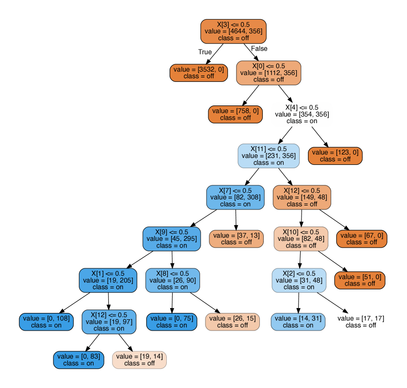
(d) GRU:10

(e) GRU:20

(f) GRU:100

(g) GRU::400

(h) GRU:800

(i) GRU:1 000

(j) GRU:10 000

Figure C.2: Decision trees trained under varying tree regularization strengths for GRU models on the signal-and-noise HMM dataset dataset. As the tree regularization increases, the number of nodes collapses to a single one. If we focus on (h), we see that the tree resembles the ground truth data-generating function quite closely.

C.3 Signal-and-noise HMM: AUCs

Model	AUC (Test)	Average Path Length	Parameter Count
logreg	0.91832	17.302	6
decision tree	0.92050	29.4424	-
hmm (5)	0.93591	25.5736	71
hmm (20)	0.94177	27.2784	581
gru (1)	0.65049	1.8876	29
gru (5)	0.94812	26.304	205
gru (6)	0.94883	27.2118	264
gru (10)	0.94962	28.563	560
gru (15)	0.93982	30.7172	1 065
gru (20)	0.93368	37.0844	1 720
grutree (20/10.0)	0.94226	28.1850	1 720
grutree (20/200.0)	0.94806	26.8140	1 720
grutree (20/7 000.0)	0.94431	22.4646	1 720
grutree (20/9 000.0)	0.90555	9.1127	1 720
grutree (20/10 000.0)	0.82770	3.4400	1 720
gruhmm (5/1)	0.95146	18.2202	100
gruhmm (5/5)	0.95584	27.258	276
gruhmm (5/10)	0.95773	30.9624	631
gruhmm (5/15)	0.94857	36.7188	1 136
gruhmmtree (5/15/1.0)	0.95382	24.115	1 136
gruhmmtree (5/15/10.0)	0.95180	16.883	1 136
gruhmmtree (5/15/50.0)	0.95258	12.573	1 136
gruhmmtree (5/15/200.0)	0.95145	8.926	1 136
gruhmmtree (5/15/500.0)	0.95769	5.231	1 136
gruhmmtree (5/15/900.0)	0.95708	3.942	1 136
gruhmmtree (5/15/2 000.0)	0.95648	2.694	1 136
gruhmmtree (5/15/5 000.0)	0.95399	1.896	1 136
gruhmmtree (5/15/7 000.0)	0.93591	0.000	1 136

Table C.1: Performance metrics across models on the signal-and-noise HMM dataset. The parameter count is included as a measure of the model capacity.

C.4 Sepsis: Plots

(a) In-Hospital Mortality

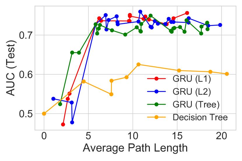
(b) 90-Day Mortality

(c) Mechanical Ventilation

(d) Median Vasopressor

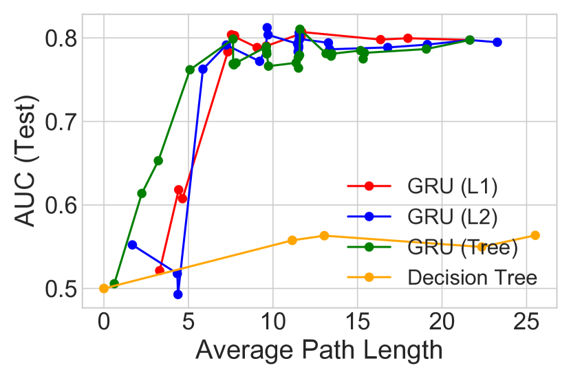
(e) Max Vasopressor

Figure C.3: Performance and complexity trade-offs using L1, L2, and Tree regularization on GRU performance on the Sepsis dataset.

C.5 Sepsis: Tree Visualization

(a) In-Hospital Mortality

(b) 90-Day Mortality

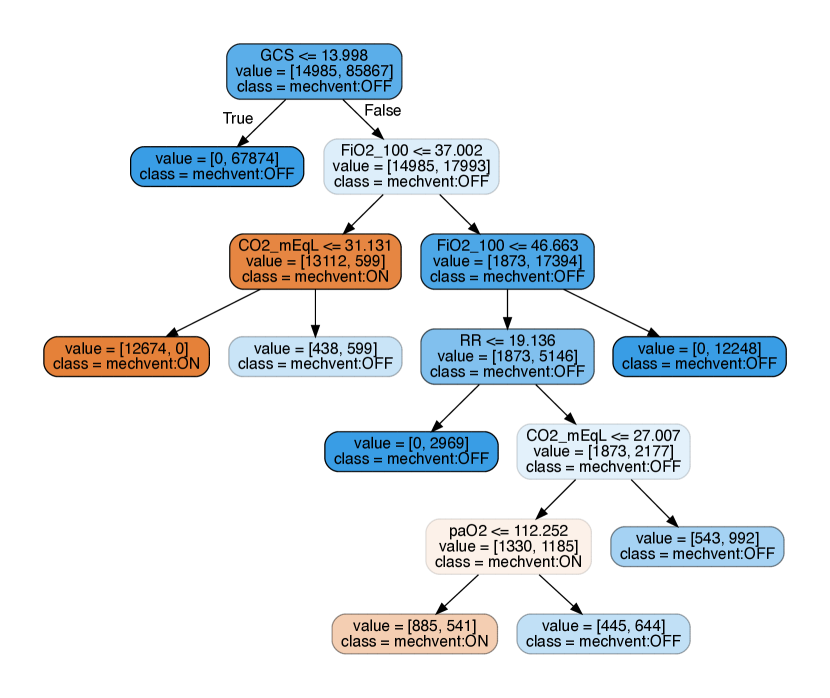
(c) Mechanical Ventilation

(d) Median Vasopressor

(e) Max Vasopressor

Figure C.4: Decision trees trained using $\lambda=800.0$ for a GRU model using Sepsis. The 5 output dimensions are jointly trained.

C.6 Sepsis: AUCs

Model	In-Hospital Mortality	90-Day Mortality	Mechanical Ventilation	Median Vasopressor	Max Vasopressor	Total Average Path Length	Parameter Count
logreg	0.6980	0.6986	0.8242	0.7392	0.7392	32.489	180
decision tree	0.7017	0.7016	0.8509	0.7439	0.7427	76.242	-
hmm (5)	0.7128	0.7095	0.6979	0.7295	0.7290	35.125	405
hmm (10)	0.7227	0.7297	0.8237	0.7409	0.7405	57.629	860
hmm (15)	0.7216	0.7282	0.8188	0.7346	0.7341	61.832	1 365
hmm (20)	0.7233	0.7350	0.8218	0.7371	0.7364	62.353	1 920
hmm (25)	0.7147	0.7321	0.8089	0.7313	0.7310	63.415	2 525
hmm (30)	0.7164	0.7297	0.8099	0.7316	0.7311	65.164	3 180
hmm (35)	0.7177	0.7237	0.8095	0.7201	0.7195	65.474	3 885
hmm (50)	0.7267	0.7357	0.8373	0.7335	0.7328	66.317	6 300
hmm (75)	0.7254	0.7361	0.8059	0.7434	0.7430	72.553	11 325
hmm (100)	0.7294	0.7354	0.8129	0.7408	0.7403	80.415	17 600
gru (1)	0.3897	0.6400	0.4761	0.7414	0.7411	31.816	117
gru (5)	0.7357	0.7296	0.8795	0.7866	0.7862	45.395	645
gru (10)	0.7488	0.7445	0.8892	0.7983	0.7979	58.102	1 440
gru (15)	0.7529	0.7450	0.8912	0.8020	0.8021	61.025	2 385
gru (20)	0.7535	0.7497	0.8887	0.8018	0.8017	61.214	3 480
gru (25)	0.7578	0.7486	0.8902	0.8113	0.8114	62.029	4 725
gru (30)	0.7602	0.7508	0.8927	0.8063	0.8061	72.854	6 120
gru (35)	0.7522	0.7483	0.8900	0.8095	0.8091	74.091	7 665
gru (50)	0.7431	0.7390	0.8895	0.8054	0.8051	76.543	13 200
gru (75)	0.7408	0.7239	0.8837	0.8006	0.8000	87.422	25 425
gru (100)	0.7325	0.7273	0.8781	0.7977	0.7975	94.161	41 400
grutree (100/0.01)	0.7276	0.7314	0.8776	0.7873	0.7867	91.797	41 400
grutree (100/1.0)	0.7147	0.7040	0.8741	0.7812	0.7810	82.019	41 400
grutree (100/8.0)	0.7232	0.7203	0.8763	0.7845	0.7840	73.767	41 400
grutree (100/20.0)	0.7123	0.7085	0.8733	0.7813	0.7813	65.035	41 400
grutree (100/70.0)	0.7360	0.7376	0.8813	0.7988	0.7986	61.012	41 400
grutree (100/300.0)	0.7210	0.7197	0.8681	0.7676	0.7678	54.177	41 400
grutree (100/2 000.0)	0.7230	0.7167	0.8335	0.7616	0.7619	48.206	41 400
grutree (100/5 000.0)	0.6546	0.6552	0.6752	0.6668	0.6530	26.085	41 400
grutree (100/7 000.0)	0.6063	0.6554	0.6565	0.6230	0.6138	20.214	41 400
grutree (100/8 000.0)	0.5298	0.5242	0.5025	0.5026	0.5057	13.383	41 400
gruhmm (1/5)	0.4222	0.6472	0.4678	0.7478	0.7477	41.583	722
gruhmm (1/10)	0.4007	0.6295	0.4730	0.7418	0.7419	61.041	1 517
gruhmm (1/25)	0.4019	0.6207	0.4773	0.7353	0.7352	65.955	4 802
gruhmm (1/50)	0.3999	0.6162	0.4772	0.7120	0.7121	70.534	13 277
gruhmm (5/5)	0.7430	0.7372	0.8798	0.8009	0.8006	47.639	1 050
gruhmm (5/10)	0.7408	0.7320	0.8819	0.7991	0.7988	63.627	1 845
gruhmm (5/25)	0.7365	0.7279	0.8776	0.7955	0.7952	68.215	5 130
gruhmm (5/50)	0.7222	0.7107	0.8660	0.7814	0.7811	71.572	13 605
gruhmm (10/5)	0.7468	0.7467	0.8949	0.8098	0.8097	50.902	1 505
gruhmm (10/10)	0.7490	0.7478	0.8958	0.8098	0.8096	63.522	2 300
gruhmm (10/25)	0.7422	0.7407	0.8916	0.8055	0.8054	70.919	5 585
gruhmm (10/50)	0.7254	0.7221	0.8824	0.7903	0.7903	71.297	14 060
gruhmm (25/5)	0.7580	0.7568	0.8941	0.8236	0.8235	51.794	3 170
gruhmm (25/10)	0.7592	0.7563	0.8945	0.8225	0.8225	64.223	3 965
gruhmm (25/25)	0.7525	0.7508	0.8912	0.8186	0.8184	72.480	7 250
gruhmm (25/50)	0.7604	0.7583	0.8954	0.8106	0.8103	79.127	11 025
gruhmm (50/5)	0.7655	0.7592	0.9006	0.8228	0.8226	64.229	6 945
gruhmm (50/10)	0.7648	0.7568	0.9003	0.8220	0.8219	69.281	7 740
gruhmm (50/25)	0.7600	0.7555	0.8981	0.8205	0.8203	85.503	11 025
gruhmm (50/50)	0.7412	0.7373	0.8910	0.8056	0.8055	101.637	19 500
gruhmmtree (50/50/0.5)	0.7432	0.7492	0.879	0.7854	0.7849	84.188	19 500
gruhmmtree (50/50/20.0)	0.7435	0.747	0.8826	0.7914	0.7906	77.815	19 500
gruhmmtree (50/50/50.0)	0.7384	0.7548	0.8914	0.7922	0.7918	71.719	19 500
gruhmmtree (50/50/200.0	0.747	0.7502	0.8767	0.7832	0.7824	69.715	19 500
gruhmmtree (50/50/300.0)	0.7539	0.7623	0.8942	0.8092	0.8091	66.9	19 500
gruhmmtree (50/50/600.0	0.7435	0.7453	0.8821	0.7909	0.7905	63.703	19 500
gruhmmtree (50/50/1 000.0)	0.7575	0.7502	0.8739	0.7882	0.7873	60.949	19 500
gruhmmtree (50/50/3 000.0)	0.7396	0.7484	0.8926	0.8013	0.8011	54.751	19 500
gruhmmtree (50/50/4 000.0)	0.7432	0.7511	0.8915	0.802	0.8024	44.868	19 500
gruhmmtree (50/50/7 000.0)	0.7308	0.7477	0.8813	0.7881	0.7882	27.836	19 500
gruhmmtree (50/50/9 000.0)	0.7132	0.7319	0.8261	0.7301	0.7299	0.0	19 500

Table C.2: Performance metrics for multi-dimensional classification on a held-out portion of the Sepsis dataset. Total Average Path Length refers to the summed average path lengths across the 5 output dimensions. Refer to Fig.  C.3 for average-path-lengths split across dimensions.

C.7 HIV:Plots

(a) Therapy Success

(b) CD4⁺ $\leq$ 200 cells/ml

(c) Adherence

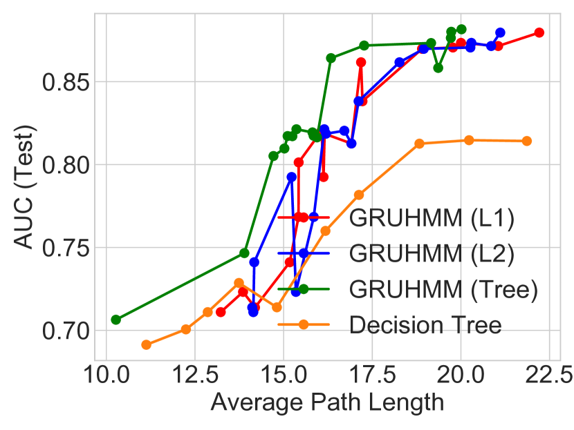
(d) Mortality

(e) Onset of AIDS

Figure C.5: Performance and complexity trade-offs using L1, L2, and Tree regularization on GRU for the HIV dataset. The 5 outputs shown here were trained jointly.

C.8 HIV: AUCs

Model	Poor Adherence	Mortality	CD4+ Count $\leq$ 200	Therapy Success	Total Average Path Length	Parameter Count
logreg	0.6884	0.7031	0.5741	0.6092	38.942	1155
decision tree	0.7100	0.7601	0.5937	0.6286	62.150	-
hmm (5)	0.7106	0.7611	0.6012	0.6265	41.864	865
hmm (10)	0.7287	0.7627	0.6237	0.6409	46.309	1780
hmm (25)	0.7243	0.7627	0.6327	0.6384	56.159	4825
hmm (50)	0.7181	0.7639	0.6412	0.6370	69.014	10900
hmm (75)	0.7244	0.7661	0.6294	0.6518	70.476	18225
hmm (100)	0.7261	0.7657	0.6287	0.6524	71.159	26800
gru (5)	0.6457	0.6814	0.6695	0.6834	58.347	1310
gru (25)	0.7516	0.7986	0.7073	0.6991	60.072	8050
gru (50)	0.7011	0.8290	0.6995	0.7054	67.513	19850
gru (75)	0.7623	0.8514	0.7117	0.7490	64.870	35400
gru (100)	0.7340	0.8216	0.6981	0.7235	67.183	54700
grutree (100/0.01)	0.7176	0.7948	0.7046	0.6803	91.020	54700
grutree (100/1.0)	0.7134	0.7997	0.7138	0.6892	86.774	54700
grutree (100/20.0)	0.7157	0.8066	0.7216	0.7114	76.025	54700
grutree (100/70.0)	0.7485	0.8210	0.7413	0.7060	68.952	54700
grutree (100/300.0)	0.7251	0.8178	0.7264	0.6746	54.058	54700
grutree (100/2 000.0)	0.7030	0.8169	0.6342	0.6627	49.839	54700
grutree (100/5 000.0)	0.6549	0.7582	0.6142	0.6352	23.895	54700
grutree (100/7 000.0)	0.6167	0.7524	0.5740	0.5634	15.283	54700
grutree (100/8 000.0)	0.5874	0.7412	0.5003	0.5027	7.391	54700
gruhmm (5/5)	0.6430	0.6647	0.5418	0.6479	67.619	2175
gruhmm (5/10)	0.6708	0.6720	0.5879	0.6517	72.137	3090
gruhmm (5/25)	0.6951	0.6981	0.6476	0.6955	68.200	6135
gruhmm (5/50)	0.6810	0.7002	0.6760	0.7114	71.518	12210
gruhmm (10/5)	0.7018	0.7147	0.7049	0.7208	64.852	3635
gruhmm (10/10)	0.7190	0.7378	0.7136	0.7578	73.252	4550
gruhmm (10/25)	0.7264	0.7457	0.7217	0.7951	70.884	7595
gruhmm (10/50)	0.7570	0.7522	0.7224	0.8234	69.726	13670
gruhmm (25/10)	0.7462	0.7861	0.7152	0.8217	68.241	9830
gruhmm (25/25)	0.7435	0.8102	0.7425	0.8186	79.261	12875
gruhmm (25/50)	0.7484	0.7714	0.7501	0.8006	76.174	18950
gruhmm (50/10)	0.7437	0.7668	0.7813	0.8260	70.081	21630
gruhmm (50/25)	0.7380	0.7557	0.7824	0.8215	88.617	24675
gruhmm (50/50)	0.7317	0.7684	0.7920	0.8007	97.864	30750
gruhmmtree (50/50/0.5)	0.7432	0.7692	0.8790	0.7804	73.168	30750
gruhmmtree (50/50/50.0)	0.7426	0.8152	0.8914	0.7979	67.729	30750
gruhmmtree (50/50/200.0	0.7461	0.8308	0.8767	0.8032	59.025	30750
gruhmmtree (50/50/600.0	0.7467	0.8820	0.8821	0.8293	52.128	30750
gruhmmtree (50/50/1 000.0)	0.7375	0.8951	0.8739	0.7882	48.247	30750
gruhmmtree (50/50/4 000.0)	0.7242	0.8461	0.8515	0.8030	14.868	30750
gruhmmtree (50/50/7 000.0)	0.7280	0.8462	0.8313	0.7484	1.836	30750

Table C.3: Performance metrics for multi-dimensional classification on a held-out portion of the HIV dataset. Total Average Path Length refers to the summed average path lengths across the output dimensions.

C.9 TIMIT:Plots/Tree Visualization

(a) TIMIT Stop Phonemes

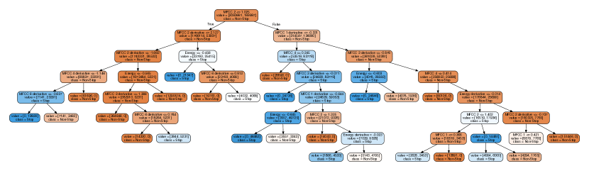
(b) GRU:500

Figure C.6: (a) Performance and complexity trade-offs using L1, L2, and Tree regularization for GRU models on TIMIT. (b) Decision tree trained using $\lambda=500.0$ tree regularization on GRU.

C.10 TIMIT:AUCs

Model	AUC	Average Path Length	Parameter Count
logreg	0.7747	23.460	27
decision tree	0.8668	59.2061	-
hmm (5)	0.8900	51.911	295
hmm (10)	0.8981	56.273	640
hmm (25)	0.9129	57.602	1 975
hmm (50)	0.9189	63.752	5 200
hmm (75)	0.9251	71.473	9 675
gru (1)	0.9169	42.602	86
gru (5)	0.9451	49.275	490
gru (10)	0.9509	60.079	1 130
gru (25)	0.9547	62.051	3 950
gru (50)	0.9578	64.957	11 650
gru (75)	0.9620	68.998	23 100
gruhmm (1/5)	0.9419	54.9723	381
gruhmm (1/10)	0.9535	53.5642	726
gruhmm (1/25)	0.9636	57.3290	2601
gruhmm (5/5)	0.9569	55.9531	785
gruhmm (5/10)	0.9575	57.6199	1 130
gruhmm (5/25)	0.9603	59.9925	2 465
gruhmm (10/5)	0.9626	57.0652	1 425
gruhmm (10/10)	0.9641	60.7877	1 770
gruhmm (10/25)	0.9651	61.0018	3 105
gruhmm (25/5)	0.9635	57.5288	4 245
gruhmm (25/10)	0.9657	60.5212	4 590
gruhmm (25/25)	0.9663	65.0161	5 925
gruhmm (50/5)	0.9676	62.2378	11 945
gruhmm (50/10)	0.9679	65.1191	12 290
gruhmm (50/25)	0.9685	67.4301	13 625
grutree (75/0.01)	0.9517	66.2801	23 100
grutree (75/0.1)	0.9466	62.4316	23 100
grutree (75/0.5)	0.9367	60.8764	23 100
grutree (75/2.0)	0.9311	58.3659	23 100
grutree (75/5.0)	0.9302	55.7588	23 100
grutree (75/10.0)	0.9288	46.6616	23 100
grutree (75/100.0)	0.8911	40.1123	23 100
grutree (75/500.0)	0.8998	28.4240	23 100
grutree (75/700.0)	0.8628	25.136	23 100
grutree (75/800.0)	0.7471	22.6671	23 100
grutree (75/1 000.0)	0.7082	17.1523	23 100
grutree (75/6 000.0)	0.5441	11.1108	23 100
grutree (75/7 000.0)	0.5088	8.9910	23 100
gruhmmtree (50/25/0.1)	0.9507	69.1110	13 625
gruhmmtree (50/25/1.0)	0.9465	67.5773	13 625
gruhmmtree (50/25/6.0)	0.9515	65.1494	13 625
gruhmmtree (50/25/20.0)	0.9449	64.0072	13 625
gruhmmtree (50/25/30.0)	0.9482	62.5406	13 625
gruhmmtree (50/25/70.0)	0.9460	58.0111	13 625
gruhmmtree (50/25/100.0)	0.9470	51.2417	13 625
gruhmmtree (50/25/500.0)	0.9401	42.1882	13 625
gruhmmtree (50/25/700.0)	0.9352	40.1281	13 625
gruhmmtree (50/25/1 000.0)	0.9390	38.0072	13 625
gruhmmtree (50/25/3 000.0)	0.9280	25.9120	13 625
gruhmmtree (50/25/4 000.0)	0.9311	21.7170	13 625
gruhmmtree (50/25/7 000.0)	0.9290	10.1122	13 625
gruhmmtree (50/25/9 000.0)	0.9134	1.0563	13 625
gruhmmtree (50/25/10 000.0)	0.9125	0.0000	13 625

Table C.4: Performance metrics across models on a held-out portion of the TIMIT dataset.

Appendix D GRU-HMM: Deep Residual Timeseries Model

Hidden Markov Model

For our purposes, Hidden Markov Models (HMMs) can be viewed as stochastic RNNs which can be interpreted as probabilistic generative models. In this work, we consider an HMM to generate a latent variable sequence $\textbf{z}=[z_{1},\ldots z_{T}]$ via a Markov chain, where each latent indicates one of $K$ possible discrete states: $z_{t}\in\left\{1,...,K\right\}$. This state sequence is then used to jointly produce the “data” $x_{t}$ and “outcomes” $y_{t}$ observed at each timestep. The joint distribution over $\textbf{z},\textbf{x},\textbf{y}$ factorizes as:

$$p(\textbf{z},\textbf{y})=\pi_{0}(z_{0})\prod_{t=1}^{T}p(z_{t}|z_{t-1},A)\cdot p(x_{t}|z_{t},\phi)\mbox{Bern}(y_{t}|\sigma(\sum_{k}w_{k}\delta_{k}(z_{t}))),$$ (6)

where $A$ is a transition matrix such that $A_{i,j}=\textup{Pr}(z_{t}=i|z_{t-1}=j)$, $\pi_{0}=p(z_{0})$ is the initial state distribution, $\left\{\phi_{k}\right\}_{k=1}^{K}$ are the emission parameters that generate data. We can then apply the same objective as above for training.

GRU-HMM: Modeling the residuals of an HMM.

We now consider an additional model, the GRU-HMM, designed for interpretability. The idea is to use a GRU to to model the residual errors when predicting the binary target via the HMM belief states. We can further penalize the complexity of the GRU predictions via our tree regularization, so that higher-quality predictions do not come at the price of a much less interpretable model.

Figure D.1: Deep residual model: GRU-HMM. The orange triangle indicates the output used in surrogate training for tree regularization.

We train the deep residual model on the same suite of synthetic and real world datasets. See Tables C.1, C.2, C.4 for a comparison of GRU-HMM with vanilla GRU and HMM models under different regularization and expressiveness parameters. We can see that across the datasets, deep residual models perform around 1% better than their vanilla equivalents with roughly the same number of model parameters.

By nature of being a residual model, decision trees were trained only on the GRU output node, leaving the HMM unconstrained. See Figure D.1 for a pictoral representation. Similar to what we did for GRU models, figures 1(b), D.2 compare model performance as the $\lambda$ parameter for L1, L2, and Tree regularization increase. We can see a similar albeit less pronounced effect where Tree regularization dominates other methods in low node count regions. It is important to notice the range of the AUC axis in these figures, where the worst the residual model can performance is the HMM-only AUC. Figure D.3 show the regularized trees produced by the GRU-HMM. Although they share some structure with Figure C.4, there are important distinctions that encourage us to conclude that the GRU in a residual models performs a different role than when trained alone.

D.1 GRU-HMM: Sepsis Plots

(a) In-Hospital Mortality

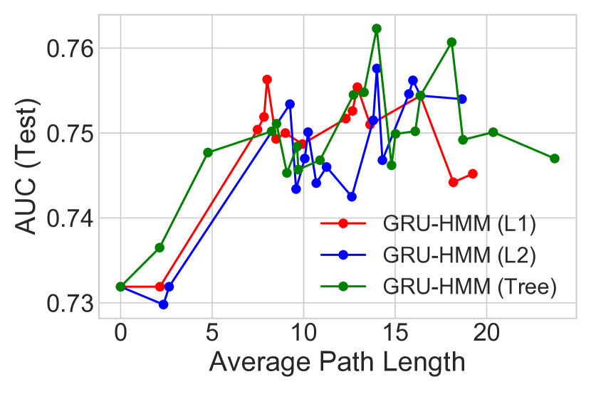
(b) 90-Day Mortality

(c) Mechanical Ventilation

(d) Median Vasopressor

(e) Max Vasopressor

Figure D.2: Performance and complexity trade-offs using L1, L2, and Tree regularization on GRU-HMM performance on the Sepsis dataset.

D.2 GRU-HMM: Sepsis Tree Visualization

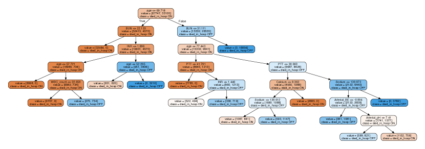
(a) In-Hospital Mortality

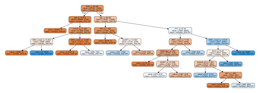
(b) 90-Day Mortality

(c) Mechanical Ventilation

(d) Median Vasopressor

(e) Max Vasopressor

Figure D.3: Decision trees trained using Tree regularization ($\lambda=2000.0$) from GRU-HMM predictions on the Sepsis dataset.

D.3 GRU-HMM: HIV Plots/Tree Visualization

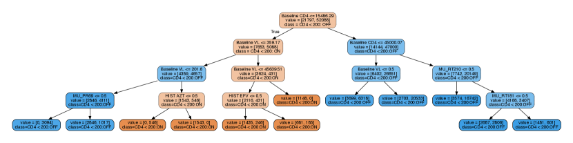
(a) GRU-HMM: CD4⁺ $\leq$ 200 cells/ml

(b) GRU-HMM: CD4⁺ $\leq$ 200 cells/ml

Figure D.4: HIV task: Study of different regularization techniques for GRU-HMM model with 75 GRU nodes and 25 HMM states, trained to predict whether CD4${+}$ $\leq$ 200 cells/ml. (a) Example decision tree for $\lambda=1000.0$. (b) Example decision tree for $\lambda=3000.0$. The tree in (b) is slightly smaller than the tree in (a) as a result of the regularisation.

D.4 GRU-HMM: TIMIT Plots/Tree Visualization

(a) GRU-HMM: Stop vs Non-Stop

(b) GRU-HMM: Stop vs Non-Stop

(c) GRU-HMM: Stop vs Non-Stop

Figure D.5: TIMIT task: Study of different regularization techniques for GRU-HMM model with 75 GRU nodes and 25 HMM states, trained to predict STOP phonemes. (a) Tradeoff curves showing how AUC predictive power and decision-tree complexity evolve with increasing regularization strength under L1, L2, or Tree regularization. (b) Example decision tree for $\lambda=3000.0$. (c) Example decision tree for $\lambda=7000.0$. When comparing with figure 6(b), this tree is significantly smaller, suggesting that the GRU performs a different role in the residual model.

Appendix E Runtime comparisons

Training Time for Tree-Regularized Models.

Table E.1 shows the wall time for training one epoch of each of the models presented in this paper using each of the datasets. Please note that the wall times for GRU-TREE and GRU-HMM-TREE include the cost of surrogate training. If the retraining frequency is small, then the amortized cost should be small.

Dataset	Model	Epoch Time (Sec.)
Signal-and-noise HMM	HMM	$16.66\pm 2.53$
Signal-and-noise HMM	GRU	$30.48\pm 1.92$
Signal-and-noise HMM	GRU-HMM	$50.40\pm 5.56$
Signal-and-noise HMM	GRU-TREE	$43.83\pm 3.84$
Signal-and-noise HMM	GRU-HMM-TREE	$73.24\pm 7.86$
SEPSIS	HMM	$589.80\pm 24.11$
SEPSIS	GRU	$822.27\pm 11.17$
SEPSIS	GRU-HMM	$1\,666.98\pm 147.00$
SEPSIS	GRU-TREE	$2\,015.15\pm 388.12$
SEPSIS	GRU-HMM-TREE	$2\,443.66\pm 351.22$
TIMIT	HMM	$1\,668.96\pm 126.96$
TIMIT	GRU	$2\,116.83\pm 438.83$
TIMIT	GRU-HMM	$3207.16\pm 651.85$
TIMIT	GRU-TREE	$3\,977.01\pm 812.11$
TIMIT	GRU-HMM-TREE	$4\,601.44\pm 805.88$

Table E.1: Training time for recurrent models measured against all datasets used in this paper. Epoch time denotes the number of seconds it took for a single pass through all the training data. The epoch times for GRU-TREE and GRU-HMM-TREE include surrogate training expenses. If we retrain sparsely, then the cost of surrogate training is amortized and the epoch time for GRU and GRU-TREE, GRU-HMM and GRU-HMM-TREE are approximately the same. To measure epoch time, we used 10 HMM states, 10 GRU states, and 5 of each for GRU-HMM models. We trained the surrogate model for 5000 epochs. These tests were run on a single Intel Core i5 CPU.

Appendix F Extended Stability Tests

In the paper, we noted that decision trees are stable over multiple run. Here, we show that using the signal-and-noise HMM dataset, 10 independent runs with random initializations and $\lambda=1000.0$ produce either the same or comparable trees. Additionally, we show that with weak regularization ($\lambda=0.01$), the variability of the learned decision trees is high. Figures F.1, F.2 include examples of such trees on the signal-and-noise dataset. Similar results are found for real-world datasets.

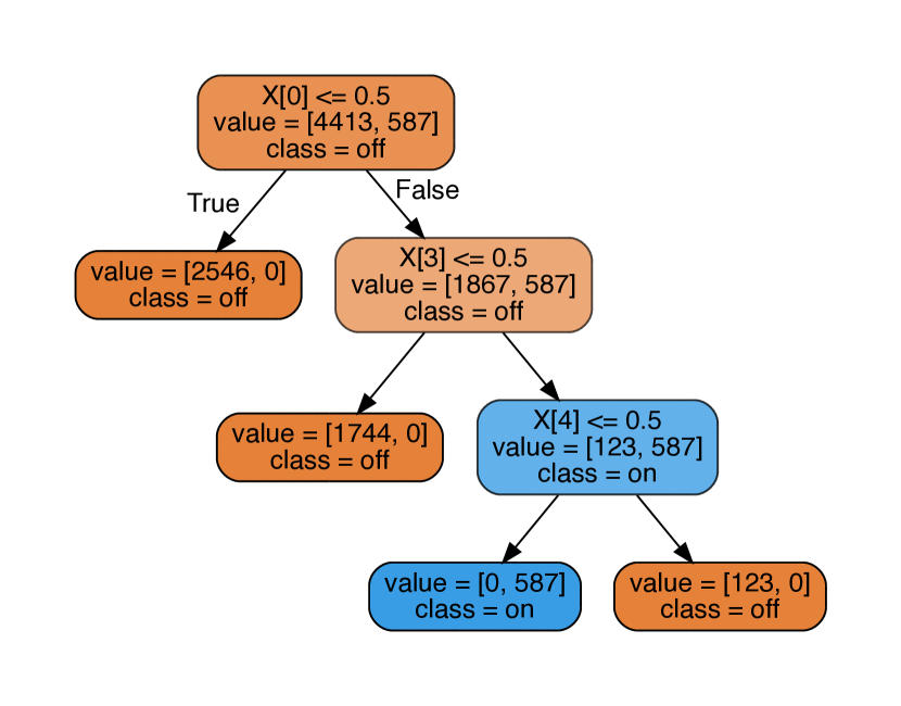
(a) 7/10 Runs

(b) 2/10 Runs

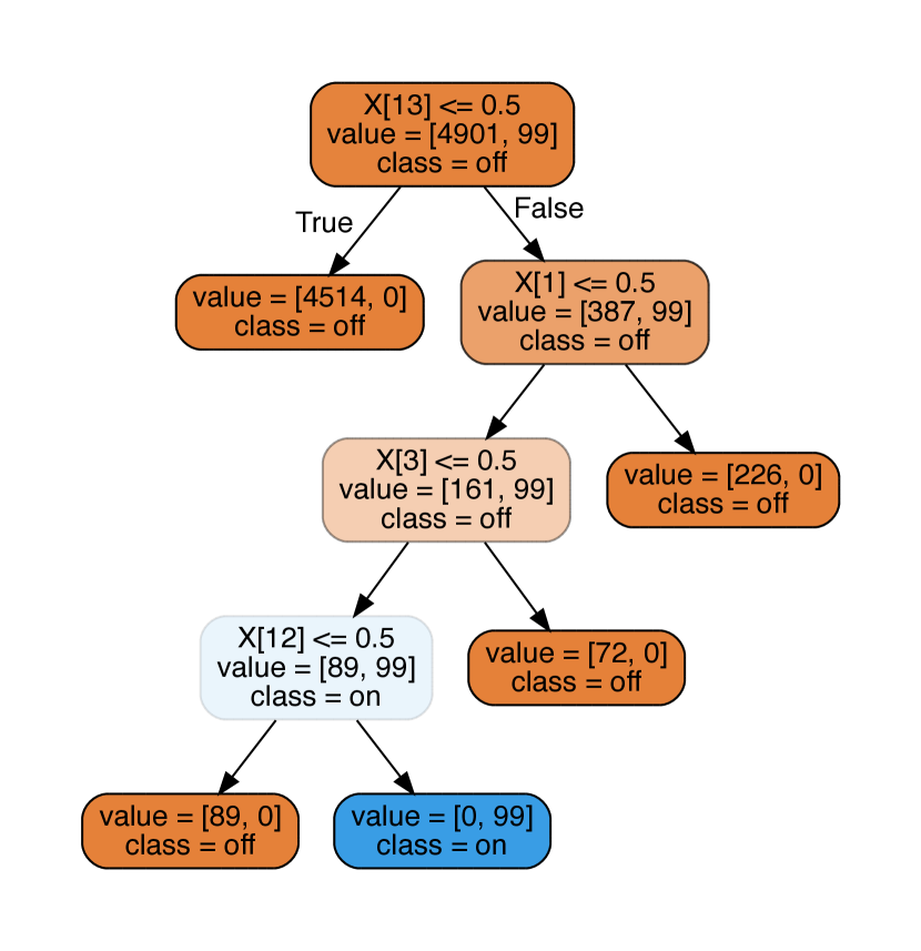
(c) 1/10 Runs

Figure F.1: Decision trees from 10 independent runs on the signal-and-noise HMM dataset with $\lambda=1000.0$. Seven of the ten runs resulted in a tree of the same structure. The other three trees are similar, often having additional subtrees but sharing the same splits and features.

(a)

(b)

(c)

(d)

Figure F.2: Decision trees from 10 independent runs on the signal-and-noise HMM dataset with $\lambda=0.01$. With low regularization, the variance in tree size and shape is high.

References

- [Adler et al. 2016] Adler, P.; Falk, C.; Friedler, S. A.; Rybeck, G.; Scheidegger, C.; Smith, B.; and Venkatasubramanian, S. 2016. Auditing black-box models for indirect influence. In ICDM.
- [Audet and Kokkolaras 2016] Audet, C., and Kokkolaras, M. 2016. Blackbox and derivative-free optimization: theory, algorithms and applications. Springer.
- [Bahdanau, Cho, and Bengio 2014] Bahdanau, D.; Cho, K.; and Bengio, Y. 2014. Neural machine translation by jointly learning to align and translate. arXiv preprint arXiv:1409.0473.
- [Balan et al. 2015] Balan, A. K.; Rathod, V.; Murphy, K. P.; and Welling, M. 2015. Bayesian dark knowledge. In NIPS.
- [Che et al. 2015] Che, Z.; Kale, D.; Li, W.; Bahadori, M. T.; and Liu, Y. 2015. Deep computational phenotyping. In KDD.
- [Chen and Asch 2017] Chen, J. H., and Asch, S. M. 2017. Machine learning and prediction in medicineâbeyond the peak of inflated expectations. N Engl J Med 376(26):2507–2509.
- [Cho et al. 2014] Cho, K.; Gulcehre, B. v. M. C.; Bahdanau, D.; Schwenk, F. B. H.; and Bengio, Y. 2014. Learning phrase representations using RNN encoder–decoder for statistical machine translation. In EMLNP.
- [Choi et al. 2016] Choi, E.; Bahadori, M. T.; Schuetz, A.; Stewart, W. F.; and Sun, J. 2016. Doctor AI: Predicting clinical events via recurrent neural networks. In Machine Learning for Healthcare Conference.
- [Craven and Shavlik 1996] Craven, M., and Shavlik, J. W. 1996. Extracting tree-structured representations of trained networks. In NIPS.
- [Drucker and Le Cun 1992] Drucker, H., and Le Cun, Y. 1992. Improving generalization performance using double backpropagation. IEEE Transactions on Neural Networks 3(6):991–997.
- [Erhan et al. 2009] Erhan, D.; Bengio, Y.; Courville, A.; and Vincent, P. 2009. Visualizing higher-layer features of a deep network. Technical Report 1341, Department of Computer Science and Operations Research, University of Montreal.
- [Garofolo et al. 1993] Garofolo, J. S.; Lamel, L. F.; Fisher, W. M.; Fiscus, J. G.; Pallett, D. S.; Dahlgren, N. L.; and Zue, V. 1993. Timit acoustic-phonetic continuous speech corpus. Linguistic data consortium 10(5).
- [Goodfellow, Bengio, and Courville 2016] Goodfellow, I.; Bengio, Y.; and Courville, A. 2016. Deep Learning. MIT Press. http://www.deeplearningbook.org.
- [Han et al. 2015] Han, S.; Pool, J.; Tran, J.; and Dally, W. 2015. Learning both weights and connections for efficient neural network. In NIPS.
- [Hinton, Vinyals, and Dean 2015] Hinton, G.; Vinyals, O.; and Dean, J. 2015. Distilling the knowledge in a neural network. arXiv preprint arXiv:1503.02531.
- [Hochreiter and Schmidhuber 1997] Hochreiter, S., and Schmidhuber, J. 1997. Long short-term memory. Neural computation 9(8):1735–1780.
- [Hu et al. 2016] Hu, Z.; Ma, X.; Liu, Z.; Hovy, E.; and Xing, E. 2016. Harnessing deep neural networks with logic rules. In ACL.
- [Johnson et al. 2016] Johnson, A. E.; Pollard, T. J.; Shen, L.; Lehman, L. H.; Feng, M.; Ghassemi, M.; Moody, B.; Szolovits, P.; Celi, L. A.; and Mark, R. G. 2016. MIMIC-III, a freely accessible critical care database. Scientific Data 3.
- [Kingma and Ba 2014] Kingma, D., and Ba, J. 2014. Adam: A method for stochastic optimization. arXiv preprint arXiv:1412.6980.
- [Krizhevsky, Sutskever, and Hinton 2012] Krizhevsky, A.; Sutskever, I.; and Hinton, G. E. 2012. ImageNet classification with deep convolutional neural networks. In NIPS.
- [Lakkaraju, Bach, and Leskovec 2016] Lakkaraju, H.; Bach, S. H.; and Leskovec, J. 2016. Interpretable decision sets: A joint framework for description and prediction. In KDD.
- [Langford, Ananworanich, and Cooper 2007] Langford, S. E.; Ananworanich, J.; and Cooper, D. A. 2007. Predictors of disease progression in hiv infection: a review. AIDS Research and Therapy 4(1):11.
- [Lei, Barzilay, and Jaakkola 2016] Lei, T.; Barzilay, R.; and Jaakkola, T. 2016. Rationalizing neural predictions. arXiv preprint arXiv:1606.04155.
- [Lipton 2016] Lipton, Z. C. 2016. The mythos of model interpretability. In ICML Workshop on Human Interpretability in Machine Learning.
- [Lundberg and Lee 2016] Lundberg, S., and Lee, S.-I. 2016. An unexpected unity among methods for interpreting model predictions. arXiv preprint arXiv:1611.07478.
- [Miotto et al. 2016] Miotto, R.; Li, L.; Kidd, B. A.; and Dudley, J. T. 2016. Deep patient: An unsupervised representation to predict the future of patients from the electronic health records. Scientific Reports 6:26094.
- [Ochiai et al. 2017] Ochiai, T.; Matsuda, S.; Watanabe, H.; and Katagiri, S. 2017. Automatic node selection for deep neural networks using group lasso regularization. In ICASSP.
- [Paterson et al. 2000] Paterson, D. L.; Swindells, S.; Mohr, J.; Brester, M.; Vergis, E. N.; Squier, C.; Wagener, M. M.; and Singh, N. 2000. Adherence to protease inhibitor therapy and outcomes in patients with hiv infection. Annals of internal medicine 133(1):21–30.
- [Pedregosa et al. 2011] Pedregosa, F.; Varoquaux, G.; Gramfort, A.; Michel, V.; et al. 2011. Scikit-learn: Machine learning in Python. Journal of Machine Learning Research 12:2825–2830.
- [Raghu et al. 2017] Raghu, A.; Komorowski, M.; Celi, L. A.; Szolovits, P.; and Ghassemi, M. 2017. Continuous state-space models for optimal sepsis treatment-a deep reinforcement learning approach. In Machine Learning for Healthcare Conference.
- [Rastegari et al. 2016] Rastegari, M.; Ordonez, V.; Redmon, J.; and Farhadi, A. 2016. XNOR-Net: ImageNet classification using binary convolutional neural networks. In ECCV.
- [Ribeiro, Singh, and Guestrin 2016] Ribeiro, M. T.; Singh, S.; and Guestrin, C. 2016. Why should I trust you?: Explaining the predictions of any classifier. In KDD.
- [Ross, Hughes, and Doshi-Velez 2017] Ross, A.; Hughes, M. C.; and Doshi-Velez, F. 2017. Right for the right reasons: Training differentiable models by constraining their explanations. In IJCAI.
- [Selvaraju et al. 2016] Selvaraju, R. R.; Das, A.; Vedantam, R.; Cogswell, M.; Parikh, D.; and Batra, D. 2016. Grad-cam: Why did you say that? visual explanations from deep networks via gradient-based localization. arXiv preprint arXiv:1610.02391.
- [Singh, Ribeiro, and Guestrin 2016] Singh, S.; Ribeiro, M. T.; and Guestrin, C. 2016. Programs as black-box explanations. arXiv preprint arXiv:1611.07579.
- [Socías et al. 2011] Socías, M. E.; Sued, O.; Laufer, N.; Lázaro, M. E.; Mingrone, H.; Pryluka, D.; Remondegui, C.; Figueroa, M. I.; Cesar, C.; Gun, A.; Turk, G.; Bouzas, M. B.; Kavasery, R.; Krolewiecki, A.; Pérez, H.; Salomón, H.; Cahn, P.; and de Seroconversión Study Group, G. A. 2011. Acute retroviral syndrome and high baseline viral load are predictors of rapid hiv progression among untreated argentinean seroconverters. Journal of the International AIDS Society 14(1):40–40.
- [Sutskever, Vinyals, and Le 2014] Sutskever, I.; Vinyals, O.; and Le, Q. V. 2014. Sequence to sequence learning with neural networks. In NIPS.
- [Tang, Hua, and Wang 2017] Tang, W.; Hua, G.; and Wang, L. 2017. How to train a compact binary neural network with high accuracy? In AAAI.
- [Zazzi et al. 2012] Zazzi, M.; Incardona, F.; Rosen-Zvi, M.; Prosperi, M.; Lengauer, T.; Altmann, A.; Sonnerborg, A.; Lavee, T.; Schülter, E.; and Kaiser, R. 2012. Predicting response to antiretroviral treatment by machine learning: the euresist project. Intervirology 55(2):123–127.
- [Zhang, Lee, and Jordan 2016] Zhang, Y.; Lee, J. D.; and Jordan, M. I. 2016. l1-regularized neural networks are improperly learnable in polynomial time. In ICML.
- [Zou and Hastie 2005] Zou, H., and Hastie, T. 2005. Regularization and variable selection via the elastic net. Journal of the Royal Statistical Society: Series B (Statistical Methodology) 67(2):301–320.