Generalized speed and cost rate in transitionless quantum driving

Abstract

Transitionless quantum driving, also known as counterdiabatic driving, is a unique shortcut technique to adiabaticity, enabling a fast-forward evolution to the same target quantum states as those in the adiabatic case. However, as nothing is free, the fast evolution is obtained at the cost of stronger driving fields. Here, given the system initially get prepared in equilibrium states, we construct relations between the dynamical evolution speed and the cost rate of transitionless quantum driving in two scenarios: one that preserves the transitionless evolution for a single energy eigenstate (individual driving), and the other that maintains all energy eigenstates evolving transitionlessly (collective driving). Remarkably, we find that individual driving may cost as much as collective driving, in contrast to the common belief that individual driving is more economical than collective driving in multilevel systems. We then present a potentially practical proposal to demonstrate the above phenomena in a three-level Landau-Zener model using the electronic spin system of a single nitrogen-vacancy center in diamond.

I Introduction

The interpretation of the energy-time uncertainty relation experienced a long period of friendly debate after the birth of quantum mechanics. It has now widely accepted that this uncertainty relation is not a statement about simultaneous events but rather about the intrinsic time scale of a quantum system in a given process to evolve to a target state MT ; ML . The minimum period of time for the dynamical process is usually specified as the quantum speed limit time (see recent reviews in Refs. QSL-review0 ; QSL-Review ). Since any realistic quantum system is subject to environmental noise Book Open , the research on the energy-time uncertainty relation has recently been extended to general open systems QSL-review0 ; QSL-Review ; QSLopen1 ; QSLopen2 ; QSLopen3 ; QSLopen4 ; QSLopen5 . This uncertainty relation between energy and time has a large variety of applications in quantum physics, such as exploration of the ultimate speed of quantum computers QC-1 ; QC-2 , the mechanism for quantum dynamical speedup speedup1 ; speedup2 ; speedup3 ; Xu1 ; speedup-exp ; Xu2 ; speedup4 ; speedup5 ; speedup6 , the ultimate bound for parameter estimation in quantum metrology metrology1 ; metrology2 , and the efficiency of charging power in quantum batteries QB .

In particular, the energy-time uncertainty relation plays a key role in understanding the principle of counterdiabatic driving Rice , or transitionless quantum driving Berry , in the realization of shortcuts to adiabaticity STA-review . This nonadiabatic (fast) protocol, which reproduces the same target state as an adiabatic (slow) process, enjoys wide applications in quantum computation and quantum thermodynamics STA-review ; STA10 ; STA11 ; STA-exp1 ; STA21 ; STA31 ; shortcuts-NV ; STA32 ; STA40 ; STA41 ; santos ; STA50 ; STA60 ; song1 ; cost ; STA61 ; NX ; speedcost ; work ; santos2 ; song2 ; STA70 . However, there is no such thing as free speedup, e.g., the superadiabatic route to the implementation of universal quantum computation is founded to be bounded by the quantum speed limit santos . Recently, a rigorous relation between the speed of quantum evolution ($v$) and the cost rate of the driving field ($\partial_{t}C$) has been constructed speedcost , indicating that instantaneous manipulation is impossible as it requires an infinite cost rate. In fact, this relation is roughly demonstrated by the energy-time uncertainty relation ($\Delta E\sim\hbar/\tau$) since the variance of energy $\Delta E$ is related to the cost rate of the driving field and $\hbar/\tau\propto v$. However, this relation is obtained in a particular case, where the driving is restricted to a particular eigenstate (individual driving). Then questions naturally arise: Will a similar relation still exist in a more general case where all energy eigenstates are simultaneously driven in a transitionless way (collective driving)? Does the cost rate of individual driving always take less consumption than the collective case? What is the relationship of the dynamical speed between individual and collective driving? The answer to these questions are of great importance and may provide deeper insight into the mechanisms of counterdiabatic driving for complex quantum systems STA-review ; STA21 ; STA32 ; STA40 .

In this work, given the system initially get prepared in equilibrium states, i.e., $\partial_{t}\rho|_{t=0}=0$ book-quantum , we construct general and concise relations (or inequality) for the speed of quantum evolution and the cost rate both in collective and individual driving cases. As a by-product, we find that the cost rate of individual driving may become as large as that of collective driving, which is contrary to the common belief that collective driving costs more than individual driving in multilevel systems. As an example, we analyze the presented theory with a three-level Landau-Zener (LZ) model and design a protocol to test the above phenomena in an electronic spin of a single nitrogen-vacancy (NV) center in diamond under current experimental conditions.

The rest of this paper is organized as follows. In Section II, we present the generalized cost-cost (Sec. IIA), speed-speed (Sec. IIB), and speed-cost (Sec. IIC) relations under individual/collective counterdiabatic driving cases. Section III is dedicated to the three-level LZ model with the theory introduced in Section II. An experimental analysis is performed in Section IV with a NV center in diamond. Finally, we close with a discussion and summary in Section V.

II Generalized speed and cost rate during transitionless driving

Consider a time-dependent Hamiltonian H$(t)$ with instantaneous eigenstates {$\left|n_{t}\right\rangle$} and eigenvalues {$E_{n}(t)$}. When $H(t)$ varies sufficiently slowly, the dynamics for the $n$th eigenstate $\left|n_{t}\right\rangle$ in the adiabatic approximation is $\left|\Psi_{n}(t)\right\rangle=\exp${$-(i/\hbar)\int_{0}^{t}dt^{\prime}E_{n}(t^{\prime})-\int_{0}^{t}dt^{\prime}\left\langle n_{t^{\prime}}|\partial_{t^{\prime}}n_{t^{\prime}}\right\rangle$}$\left|n_{t}\right\rangle$. The central goal of transitionless driving is to find an auxiliary Hamiltonian $H^{A}(t)$ such that $\left|\Psi_{n}(t)\right\rangle$ becomes the exact dynamical solution of the Schrödinger equation $i\hbar\partial_{t}\left|\Psi_{n}(t)\right\rangle=\mathcal{H}(t)\left|\Psi_{n}(t)\right\rangle$, where $\mathcal{H}(t)=H(t)+H^{A}(t)$. According to the transitionless tracking algorithm, $H^{A}(t)$ can be constructed as follows Berry ,

$$H^{A}(t)=i\hbar\sum_{n}\partial_{t}(\left|n_{t}\right\rangle\left\langle n_{t}\right|)\cdot\left|n_{t}\right\rangle\left\langle n_{t}\right|.$$ (1)

We remark that the driving in Eq. (1) guarantees that all energy eigenstates evolve transitionlessly. For convenience, we call Eq. (1) collective driving. However, this strong requirement can be relaxed when we focus on a single particular eigenstate, e.g., the $n$th eigenstate $\left|n_{t}\right\rangle$, to ensure that only this eigenstate is driven transitionlessly. In other words, we may decouple the $n$th eigenstate from the rest eigenstates, and the corresponding auxiliary driving Hamiltonian is modified as Rice ; cost ; speedcost

$$H_{n}^{A}(t)=i\hbar\left[\partial_{t}(\left|n_{t}\right\rangle\left\langle n_{t}\right|),\left|n_{t}\right\rangle\left\langle n_{t}\right|\right],$$ (2)

which is hereinafter called individual driving for simplicity Note . Here the notation $[\cdot,\cdot]$ denotes the commutator and the subscript $n$ represents the individual driving for the $n$th eigenstate.

II.1 Cost rate

A series of cost functions for transitionless driving have recently been introduced, among which the simplest member, ignoring the set-up constant, possesses the following form speedcost ; cost

$$C_{(n)}=\int_{0}^{t}dt^{\prime}\left\|H_{(n)}^{A}(t^{\prime})\right\|^{\alpha},$$ (3)

where $\left\|X\right\|=\sqrt{\text{tr}\left(X^{{\dagger}}X\right)}$ is the Frobenius norm of operator $X$, and the superscript $\alpha$ depends on the nature of the driving field. For simplicity, we focus on the cost rate of transitionless driving, i.e., $\partial_{t}C_{(n)}=\left\|H_{(n)}^{A}(t)\right\|^{\alpha}$. Through straightforward calculations with Eq. (3), we obtain the cost rate for driving all energy eigenstates as

$$\partial_{t}C=\hbar^{\alpha}\left[\sum_{n}(\langle\partial_{t}n_{t}|\partial_{t}n_{t}\rangle+\langle n_{t}|\partial_{t}n_{t}\rangle^{2})\right]^{\alpha/2}$$ (4)

and for driving a particular single eigenstate as

$$\partial_{t}C_{n}=\hbar^{\alpha}\left[2\left(\langle\partial_{t}n_{t}|\partial_{t}n_{t}\rangle+\langle n_{t}|\partial_{t}n_{t}\rangle^{2}\right)\right]^{\alpha/2}.$$ (5)

Thus, it is easy to see that the relation between the collective cost rate and the individual cost rate is given by

$$\partial_{t}C=\left[\frac{1}{2}\sum_{n}(\partial_{t}C_{n})^{2/\alpha}\right]^{\alpha/2}.$$ (6)

This relation implies that the individual driving cost rate may become as large as the collective case. For instance, we have $\partial_{t}C_{k}=\partial_{t}C$ when the condition

$$\partial_{t}C_{k}=\left[\sum_{n\neq k}\left(\partial_{t}C_{n}\right)^{2/\alpha}\right]^{\alpha/2}$$ (7)

is satisfied Note2 . Note that for $n=2$, the above condition $\partial_{t}C_{1}=\partial_{t}C_{2}$ is met automatically Note , i.e., the cost rate of individual driving is equivalent to the collective case ($\partial_{t}C=\partial_{t}C_{1}=\partial_{t}C_{2}$) for any two energy level systems.

II.2 Dynamical speed from the perspective of geometry

Characterizing the dynamical speed from the perspective of geometry is intuitionistic. Before we introduce the geometric method to define the dynamical speed of quantum evolution, it is beneficial to recall the definition of the instantaneous speed $v$ of an object in three-dimensional Euclidean space with Cartesian coordinate system $v=\partial_{t}s$, where $s$ is the length of the trajectory with the line element $ds^{2}=dx^{2}+dy^{2}+dz^{2}$. Analogous to the above definition, it is very natural to define the “speed” of quantum evolution in the space of quantum states (parameterized by $\{\sigma^{\mu}\}$) as

$$v=\partial_{t}s=\sqrt{g_{\rho}},\text{ }$$ (8)

where the line element $ds^{2}=g_{\mu\nu}d\sigma^{\mu}d\sigma^{\nu}$ and $g_{\rho}=g_{\mu\nu}\partial_{t}\sigma^{\mu}\partial_{t}\sigma^{\nu}$ book-dg ; book-gs . The repeated Greek indices represent summation and $g_{\mu\nu}$ is the corresponding metric. In this paper, we adopt the quantum Fisher information metric Note3 , which is related to the distance between quantum states $\rho_{t}$ and $\rho_{t+dt}$ measured by fidelity: $F\left(\rho_{t},\rho_{t+dt}\right)=$tr$\left[\sqrt{\sqrt{\rho_{t}}\rho_{t+dt}\sqrt{\rho_{t}}}\right]\simeq 1-(1/2)g_{\rho}dt^{2}$ fidelity ; Caves . By employing the spectral decomposition of quantum state $\rho_{t}=\sum_{j}p_{j}\left|j\right\rangle\left\langle j\right|,$ $g_{\rho}$ can be written in an explicit form book-gs ; fidelity ; Caves

$$g_{\rho}=\frac{1}{4}\sum_{j}\frac{(\partial_{t}p_{j})^{2}}{p_{j}}+\frac{1}{2}\sum_{j\neq l}\frac{(p_{j}-p_{l})^{2}}{p_{j}+p_{l}}\left|\left\langle j_{t}|\partial_{t}l_{t}\right\rangle\right|^{2}.$$ (9)

It is easy to check that if the state is pure, e.g., $\rho_{t}=\left|\Phi_{t}\right\rangle\left\langle\Phi_{t}\right|,$ Eq. (9) reduces to

$$g_{\Phi}=\frac{\left|\left\langle\partial_{t}\Phi_{\perp}|\partial_{t}\Phi_{t}\right\rangle\right|^{2}}{\left\langle\partial_{t}\Phi_{\perp}|\partial_{t}\Phi_{\perp}\right\rangle},$$ (10)

where the unnormalized state $\left|\partial_{t}\Phi_{\perp}\right\rangle=\left|\partial_{t}\Phi_{t}\right\rangle-\left\langle\Phi_{t}|\partial_{t}\Phi_{t}\right\rangle\left|\Phi_{t}\right\rangle$ is the component of $\left|\partial_{t}\Phi_{t}\right\rangle$ orthogonal to $\left|\Phi_{t}\right\rangle$ Caves ; Xu .

For simplicity, we consider the initial states get prepared in equilibrium, i.e., $\partial_{t}\rho|_{t=0}=0$ book-quantum . Therefore, $\rho_{0}$ and $H$ can be simultaneously diagonalized, thus providing the possibilities to establish a link between cost rate and speed of evolution. We first consider an initial state in the form of canonical ensemble $\rho_{0}=\exp[-H(0)/(kT)]/Z=\sum_{n}p_{n}\left|n_{0}\right\rangle\left\langle n_{0}\right|$, where $Z=$tr$[e^{-H(0)/(kT)}]$ is the partition function with temperature $T$, $k$ is the Boltzmann constant, and $p_{n}=\exp[-E_{n}(0)/(kT)]/Z$ book-quantum . We remark that under transitionless driving, $p_{n}$ is time-independent, i.e., $\partial_{t}p_{n}=0$. Therefore, Eq. (9) reduces to

$$g_{\rho}=\frac{1}{2}\sum_{m\neq n}\frac{\left(p_{m}-p_{n}\right)^{2}}{p_{m}+p_{n}}|\left\langle m_{t}|\partial_{t}n_{t}\right\rangle|^{2}.$$ (11)

As a special case when the system is initially in the $n$th eigenstate $\left|n_{0}\right\rangle$, according to Eq. (10), the quantum Fisher information metric continuously reduces to the well-known Fubini–Study metric as follows:

$$g_{n} = \frac{\left|\langle\partial_{t}n_{\perp}|\partial_{t}n_{t}\rangle\right|^{2}}{\langle\partial_{t}n_{\perp}|\partial_{t}n_{\perp}\rangle},$$ (12)

$$= \langle\partial_{t}n_{t}|\partial_{t}n_{t}\rangle+\langle n_{t}|\partial_{t}n_{t}\rangle^{2},$$

where $\left|\partial_{t}n_{\perp}\right\rangle=\left|\partial_{t}n_{t}\right\rangle-\left\langle n_{t}|\partial_{t}n_{t}\right\rangle|n_{t}\rangle$.

Here, it is convenient to establish a relation of quantum speed between the collective and the individual driving. According to Eqs. (8), (11), and (12) we have

$$v = \sqrt{\frac{1}{2}\sum_{m\neq n}\frac{\left(p_{m}-p_{n}\right)^{2}}{p_{m}+p_{n}}|\left\langle m_{t}|\partial_{t}n_{t}\right\rangle|^{2}},$$ (13)

$$\leq \sqrt{\frac{1}{2}\sum_{m\neq n}(p_{m}+p_{n})|\left\langle m_{t}|\partial_{t}n_{t}\right\rangle|^{2}},$$

$$= \sqrt{\sum_{m\neq n}p_{n}|\left\langle m_{t}|\partial_{t}n_{t}\right\rangle|^{2}},$$

$$= \sqrt{\sum_{n}p_{n}\left(\langle\partial_{t}n_{t}|\partial_{t}n_{t}\rangle+\langle n_{t}|\partial_{t}n_{t}\rangle^{2}\right)},$$

$$= \sqrt{\sum_{n}p_{n}(v_{n})^{2}},$$

where $v_{n}=\sqrt{\langle\partial_{t}n_{t}|\partial_{t}n_{t}\rangle+\langle n_{t}|\partial_{t}n_{t}\rangle^{2}}$. Note that $\left(p_{m}-p_{n}\right)^{2}\leq\left(p_{m}+p_{n}\right)^{2}$ is employed in the second line of Eq. (13), and the equality in the second line is achieved when the system is initially prepared in a single eigenstate.

II.3 Relationship between cost rate and dynamical speed

Clearly, with Eqs. (5), (8), and (12), the cost rate and the dynamical speed of transitionless quantum driving for a single eigenstate $\left|n_{t}\right\rangle$ is obtained as

$$v_{n}=\frac{\sqrt[\alpha]{\partial_{t}C_{n}}}{\sqrt{2}\hbar}.$$ (14)

We note that the above relation bears resemblance to the speed and the cost rate relation first presented in Ref. speedcost but in a more concise form. However, the relation between the cost rate and the dynamical speed by collective transitionless driving is not as concise as Eq. (14). For the collective transitionless driving case ($n\geq 2$), with Eqs. (4) and (13), we have

$$v < \sqrt{\sum_{n}(\langle\partial_{t}n_{t}|\partial_{t}n_{t}\rangle+\langle n_{t}|\partial_{t}n_{t}\rangle^{2})}$$ (15)

$$= \frac{\sqrt[\alpha]{\partial_{t}C}}{\hbar}.$$

Equations (6), (13), (14), and (15), which reflect the general relations between the dynamical speed and the cost rate in shortcuts to adiabaticity for both collective and individual transitionless driving, are the main contributions in this paper. The properties of these relations are explored in the following pedagogical nontrivial example.

III Three-level Landau-Zener tunneling model

In this section, we consider the Landau-Zener tunneling model in the simplest multilevel system, i.e., the three-level system, with the following Hamiltonian

$$H(t)=\gamma_{e}\mathbf{B}(t)\cdot\mathbf{S},$$ (16)

where $\gamma_{e}$ is the electronic gyromagnetic ratio, $\mathbf{B}(t)=\{\Delta,0,\lambda(t)\}/\gamma_{e}$ is the magnetic field applied along the $x$ and $z$ directions, and $\mathbf{S}=${$S_{x},S_{y},S_{z}$} is the $S=1$ electron spin operator spin . Here $\Delta$ denotes the minimum energy separation and $\lambda(t)$ characterizes the strength of a controllable driving field.

According to the method introduced in Ref. Berry , it is convenient to validate that the collective transitionless driving for Eq. (16) is given by

$$H^{A}(t)=V(t)S_{y},$$ (17)

with $V(t)=-\Delta\partial_{t}\lambda(t)/[\Delta^{2}+\lambda^{2}(t)]$, which is similar to the two-level case Berry ; shortcuts-NV . The given control field is scanned linearly within $t\in[0,\tau],$ i.e., $\lambda(t)=\kappa(2t/\tau-1),$ where $\kappa$ is related to the strength of the driving field. Considering the nature of the applied fields, we adopt the parameter $\alpha=2$ cost for evaluating the cost rate of transitionless driving.

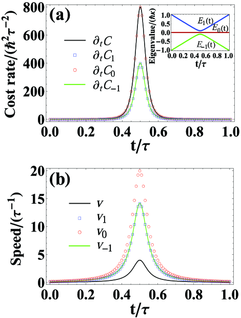
Figure 1: (Color online) (a) The cost rate (divided by $\hbar^{2}\tau^{-2}$) of collective ($\partial_{t}C$) and individual ($\partial_{t}C_{1},\partial_{t}C_{0},\partial_{t}C_{-1}$) transitionless quantum driving for the three-level LZ model evolved through the avoided crossing by $\lambda(t)=\kappa(2t/\tau-1)$, and $\Delta/\kappa=0.1$. The inset shows the energy eigenvalues (divided by $\hbar\kappa$) of the LZ model of Eq. (16) with the above parameters. (b) The corresponding speed (divided by $\tau^{-1}$) of states under collective and individual transitionless driving. For collective driving, we have set $\hbar\kappa/(kT)=1/2$ for the initial canonical ensemble state as an example.

We first employ the above driving protocol to analyze the collective and individual cost rates during transitionless quantum driving. The results are shown in Fig. 1(a) with $\Delta/\kappa=0.1$ as an example. In general, the peaks in Fig. 1(a) illustrate that more resources or higher cost rates are required to realize transitionless driving in the neighborhood of an avoided crossing. Obviously, the individual driving of eigenstates $E_{\pm 1}(t)$ costs less than the collective driving, which can easily be understood in terms of Eqs. (4) and (5) as $\partial_{t}C_{+1}=\partial_{t}C_{-1}=(1/2)\partial_{t}C_{0}<\partial_{t}C$. However, an interesting phenomenon occurs. The individual driving for eigenstate $E_{0}(t)$ (red circle) costs as much as the collective driving (black curve), in contrast to the common belief that the individual transitionless driving leads to less consumption for multilevel quantum systems. In fact, since $\partial_{t}C_{0}=2\partial_{t}C_{\pm 1}=\partial_{t}C_{+1}+\partial_{t}C_{-1}$, which is just the condition of Eq. (7) in the three level case. Therefore, we have $\partial_{t}C=\partial_{t}C_{0}$. Physically, this can be interpreted by means of the configuration of eigenstates in Eq. (16) shown in the insets of Fig. 1(a). In order to achieve the individual driving of $E_{0}(t)$, transitions from $E_{0}(t)$ to both $E_{-1}(t)$ and $E_{1}(t)$ should be avoided. In turn, the eigenstates $E_{\pm}(t)$ will not transit to $E_{0}(t)$, and their mutual transitions are prohibited, which is the principle of collective driving.

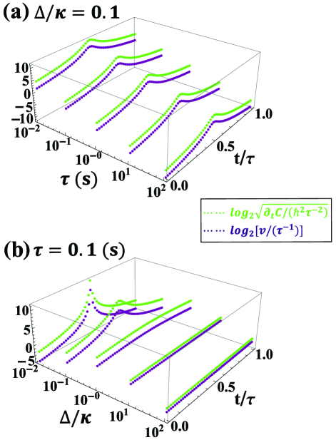
Figure 2: (Color online) Time dependence of the dimensionless cost rate log${}_{2}\sqrt{\partial_{t}C/(\hbar^{2}\tau^{-2})}$ and speed log${}_{2}[v/(\tau^{-1})]$ during collective transitionless quantum driving for the three-level LZ model. (a) Different choices of time duration $\tau$ with fixed energy splitting $\Delta/\kappa=0.1$. (b) Various energy splitting $\Delta$ with fixed time duration $\tau=0.1$ $(s)$. All other parameters are the same as in Fig. 1.

In addition, the tendency between the cost rate and the speed can be seen by comparison with Fig. 1(b), where the instantaneous speed of states for the above two scenarios is depicted. We note that although the cost rates for the collective driving ($\partial_{t}C$) and the individual driving ($\partial_{t}C_{0}$) are equal in this model, the corresponding dynamical speed does not possess such a property, i.e., $v<v_{0}$ [see in Fig. 1(b)].

We then examine the instantaneous cost rate and the speed under transitionless driving with different driving time durations $\tau$ and energy splittings $\Delta$. For convenience, we focus on the collective driving, and the values are reported in the form of base-2 logarithm. As clearly shown in Fig. 2(a), if the energy splitting is fixed, e.g., $\Delta/\kappa=0.1$, a higher cost rate is required to rapidly go through the avoided crossing with a faster dynamical speed to realize the transitionless driving, which is in agreement with Eq. (15). When approaching the adiabatic limit, e.g., $\tau=100$ (s), almost no transitionless driving is needed ($\partial_{t}C\rightarrow 0$). On the other hand, if the energy splitting $\Delta$ is sufficiently large, e.g., $\Delta/\kappa=100$ in Fig. 2(b), only a little cost is required to achieve the transitionless driving.

IV Possible experimental realization using NV centers in diamond

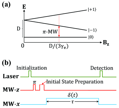
Figure 3: (Color online) (a) The energy-level diagram for the electronic spin ground triplet state of a single NV center with a zerofield splitting $D$. A polarized $\pi-$MW pulse is performed on $\left|0\right\rangle$ and $\left|-1\right\rangle$ at $B_{z}=D/(3\gamma_{e})$ to achieve the required Hamiltonian $H_{NV}(t)=\omega_{0}S_{z}$ with $\omega_{0}=2D/3$. (b) Diagram of the schematic experimental pulse sequences employed to realize the three level LZ model under tranistionless driving. The electronic spin state is initialized by 532 nm laser. The initial equilibrium states can be prepared by a serial of MW pulses. Then a microwave field $B_{x}(t)=\delta(t)/\gamma_{e}$ with $\delta(t)=2[\Delta\cos\varepsilon(t)-V(t)\sin\varepsilon(t)]$ and $\partial_{t}\varepsilon(t)=\omega_{0}-$ $\lambda(t)$, is performed along the $x$-axis of the NV center. Tomography is then performed if we would like to detect the instantaneous speed and cost rate ($\tau$ is short enough). We may also roughly estimate the average speed $\bar{v}$ by only record the time duration $\tau$ (relatively long) of the $B_{x}(t)$ performed on the electronic spin, since $\tau\varpropto 1/\bar{v}$, where $\bar{v}=(1/\tau)\int_{0}^{\tau}dt^{\prime}v.$

The NV center spins in diamond possess long coherence time at room temperature and high sensitivity to external signals. These properties make the NV center a promising candidate for quantum computation NV-Review1 and quantum sensors NV-Review2 . Here, we first outline a possible implementation of detecting the collective cost rate of transitionless driving and the dynamical speed for the three-level LZ model by using the electron spin of a single NV center in diamond. The key procedures includes the preparation of initial states, the realization of the three-level LZ Hamiltonian under transitionless driving, i.e., Eqs. (16) and (17), and the detection of speed and cost rate.

We first apply a static magnetic field to the [111] axis (taken as the $z$-axis) of the NV center and employ the ground electronic spin state $\left|-1\right\rangle,$ $\left|0\right\rangle,$ and $\left|+1\right\rangle$ as the qutrit. According to Eq. (16), it is convenient to check that the energy eigenstates of the initial three-level LZ Hamiltonian are just $\left|-1\right\rangle,$ $\left|0\right\rangle,$ and $\left|+1\right\rangle$. Therefore, preparation of an initial single energy eigenstate is achievable by microwave (MW) pulses LZS-NV ; LZS-NV2 . For an initial canonical ensemble, it can be prepared by waiting for a certain time for the dephasing from a superposition state ion . On the other hand, the Hamiltonian describing the electronic spin of the NV center takes the form NV-Review1 ; NV-Review2

$$H_{NV}(t)=DS_{z}^{2}/\hbar+\gamma_{e}B_{z}S_{z},$$ (18)

where the zero-field splitting $D=2.870$ (GHz), and the electronic gyromagnetic ratio $\gamma_{e}=28.02$ (GHz/T). We select $B_{z}=D/(3\gamma_{e})$ and apply a polarized $\pi-$MW pulse on $\left|0\right\rangle$ and $\left|-1\right\rangle$ after biasing all three energy levels by $2\hbar D/3$. Then, Eq. (18) reduces to $H_{NV}(t)=\omega_{0}S_{z}$ with $\omega_{0}=2D/3$ [see Fig. 3(a)]. According to Eqs. (16) and (17), as long as we select appropriate $\lambda(t)$ and $V(t)$, the collective transitionless driving is immediately achievable. However, the LZ avoided crossing cannot be realized directly by electron spin resonance because it requires the microwave strength approaching $4D/(3\gamma_{e})\simeq 0.137$ (T), far beyond the current experimental conditions LZS-NV ; LZS-NV2 ; shortcuts-NV . In light of the method introduced in Refs. LZS-NV ; LZS-NV2 ; shortcuts-NV , our collective transitionless driving for a three-level LZ model can also be realized in a rotating frame if we apply a microwave field $B_{x}(t)=\delta(t)/\gamma_{e}$, where $\delta(t)=2[\Delta\cos\varepsilon(t)-V(t)\sin\varepsilon(t)]$ and $\partial_{t}\varepsilon(t)=\omega_{0}-$ $\lambda(t)$, along the $x$-axis of the NV center. Thus, the total Hamiltonian in the laboratory frame is $\mathcal{H}(t)=\gamma_{e}B_{x}(t)S_{x}+\omega_{0}S_{z}$. By transferring to the rotating frame with $U=$exp$[i\varepsilon(t)S_{z}/\hbar]$, we obtain

$$\mathcal{\tilde{H}}(t) = UH(t)U^{{\dagger}}+i\hbar(\partial_{t}U)U^{{\dagger}},$$ (19)

$$= \lambda(t)S_{z}+U\delta(t)S_{x}U^{{\dagger}},$$

$$\simeq \Delta S_{x}+V(t)S_{y}+\lambda(t)S_{z},$$

where a rotating wave approximation, ignoring the fast-oscillating items exp[$\pm 2i\varepsilon(t)$], is employed in the deduction of the third line. Clearly, the above equation yields the exact Hamiltonian presented in Eqs. (16) and (17). In this rotating frame, $\Delta$ and $\lambda(t)$ are, respectively, controlled by the power and frequency of the microwave field in the $x$-axis, which in turn determines the corresponding counterdiabatic field $V(t)$. Thus, the cost rate of the transitionless quantum driving field and the speed of evolution can be completely controlled the microwave field $B_{x}(t)$. According to Eqs. (4) and (13), the detection of the speed and cost rate in experiment is flexible, which can be realized by the tomography of instantaneous density matrix. In addition, even with no tomography, we can also roughly estimate the average speed of quantum evolution by detecting the duration of the evolved time $\tau$, since $\tau\varpropto 1/\bar{v}$, where $\bar{v}=(1/\tau)\int_{0}^{\tau}dt^{\prime}v$. A diagram of the above schematic experimental pulse sequences is depicted in Fig. 3(b).

Because the individual transitionless driving is equivalent to a collectively driving two-level system cost ; Note ; thus, the corresponding experimental methods can refer to the two-level case in Ref. shortcuts-NV . Together with above analysis, the phenomenon that cost rate of individual driving may be as large as collective driving can also be verified with above three-level LZ model in NV centers.

V DISCUSSIONS AND CONCLUSIONS

Though our present example mainly focuses on a three-level LZ model, the cost rate and speed relations of collective driving and individual driving presented in Sec. II are applicable to any multilevel systems. Therefore, further study on more complicated multilevel ($n\geq 4$) physical systems will be of great interest and importance in the field of shortcuts to adiabaticity. On the other hand, quantum thermodynamics processes of experimental implementation at the fundamental level of a single spin is now emerging, e.g., a single-spin test with a single ultracold ⁴⁰Ca⁺ trapped ion has been employed to verify the Jarzynski-Related information equality ion . Therefore, in addition to NV centers, it would also be desirable and interesting to further investigate our theory with trapped ion systems in experiment.

In summary, general relations between the dynamical speed and the cost rate of individual/collective transitionless driving have been constructed, which provide a unified way to explore the cost-cost, speed-speed, and speed-cost relations under individual/collective counterdiabatic driving. In particular, the counterintuitive phenomenon that the cost rate of individual driving can be as large as the corresponding collective driving in multilevel systems has been discovered and illustrated in a three-level LZ model. We have also proposed a possible experimental verification of this phenomenon in the electron spin of a single NV center in diamond. We expect these studies to contribute to the identification of the physical mechanisms for the costs of shortcuts to adiabaticity and its experimental examination in simple/complex quantum systems.

References

- (1) L. Mandelstam and I. Tamm, J. Phys. (USSR) 9, 249 (1945).
- (2) N. Margolus and L. B. Levitin, Phys. D 120, 188(1998).
- (3) M. R. Frey, Quantum Inf. Process. 15, 3919 (2016).
- (4) S. Deffner and S. Campbell, J. Phys. A, 50, 453001 (2017).
- (5) H.-P. Breuer and F. Petruccione, The Theory of Open Quantum Systems (Oxford University Press, Oxford, 2007).
- (6) M. M. Taddei, B. M. Escher, L. Davidovich, and R. L. de Matos-Filho, Phys. Rev. Lett. 110, 050402 (2013).
- (7) A. del Campo, I. L. Egusquiza, M. B. Plenio, and S. F. Huelga, Phys. Rev. Lett. 110, 050403 (2013).
- (8) S. Deffner and E. Lutz, Phys. Rev. Lett. 111, 010402 (2013).
- (9) I. Marvian and D. A. Lidar, Phys. Rev. Lett. 115, 210402 (2015).
- (10) D. P. Pires, M. Cianciaruso, L. C. Céleri, G. Adesso, D. O. Soares-Pinto, Phys. Rev. X 6, 021031 (2016).
- (11) S. Lloyd, Nature (London) 406, 1047 (2000).
- (12) I. L. Markov, Nature (London) 512, 147 (2014).
- (13) V. Giovannetti, S. Lloyd, and L. Maccone, Phys. Rev. A 67, 052109 (2003).
- (14) J. Batle, M. Casas, A. Plastino, and A. R. Plastino, Phys. Rev. A 72, 032337 (2005).
- (15) A. Borras, M. Casas, A. R. Plastino, and A. Plastino, Phys Rev. A 74, 022326 (2006).
- (16) Z.-Y. Xu, S. Luo, W. L. Yang, C. Liu, and S. Zhu, Phys. Rev. A 89, 012307 (2014).
- (17) A. D. Cimmarusti, Z. Yan, B. D. Patterson, L. P. Corcos, L. A. Orozco, and S. Deffner, Phys. Rev. Lett. 114, 233602 (2015).
- (18) C. Liu, Z.-Y. Xu, and S. Zhu, Phys. Rev. A 91, 022102 (2015).
- (19) Y.-J. Zhang, W. Han, Y.-J. Xia, J.-P. Cao, and H. Fan, Phys. Rev. A 91, 032112 (2015).
- (20) H.-B. Liu, W. L. Yang, J.-H. An, and Z.-Y. Xu, Phys. Rev. A 93, 020105(R) (2016).
- (21) X. Cai and Y. Zheng, Phys. Rev. A 95, 052104 (2017).
- (22) V. Giovanetti, S. Lloyd, and L. Maccone, Nat. Photon. 5, 222 (2011).
- (23) A. W. Chin, S. F. Huelga, and M. B. Plenio, Phys. Rev. Lett. 109, 233601 (2012).
- (24) F. Campaioli, F. A. Pollock, F. C. Binder, L. Céleri, J. Goold, S. Vinjanampathy, and K. Modi, Phys. Rev. Lett. 118, 150601 (2017).
- (25) M. Demirplack and S. A. Rice, J. Chem. Phys. 129, 154111 (2008).
- (26) M. Berry, J. Phys. A 42, 365303 (2009).
- (27) E. Torrontegui, S. S. Ibáñez,, S. Martínez-Garaot, M. Modugno, A. del Campo, D. Guéry-Odelin, A. Ruschhaupt, X. Chen, and J. G. Muga, Adv. At. Mol. Opt. Phys. 62, 117 (2013).
- (28) X. Chen, I. Lizuain, A. Ruschhaupt, D. Guéry-Odelin, and J. G. Muga, Phys. Rev. Lett. 105, 123003 (2010).
- (29) J. G. Muga, X. Chen, S. Ibáñez, I. Lizuain, and A. Ruschhaupt, J. Phys. B 43, 085509 (2010).
- (30) M. G. Bason, M. Viteau, N. Malossi, P. Huillery, E. Arimondo, D. Ciampini, R. Fazio, V. Giovannetti, R. Mannella, and O. Morsch, Nat. Phys. 8, 147 (2011).
- (31) A. del Campo, M. M. Rams, and W. H. Zurek, Phys. Rev. Lett. 109, 115703 (2012).
- (32) C. Jarzynski, Phys. Rev. A 88, 040101(R) (2013).
- (33) J. Zhang, J. H. Shim, I. Niemeyer, T. Taniguchi, T. Teraji, H. Abe, S. Onoda, T. Yamamoto, T. Ohshima, J. Isoya, and D. Suter, Phys. Rev. Lett. 110, 240501 (2013).
- (34) A. del Campo, Phys. Rev. Lett. 111, 100502 (2013).
- (35) S. Deffner, C. Jarzynski, and A. del Campo, Phys. Rev. X 4, 021013 (2014).
- (36) G. Vacanti, R. Fazio, S. Montangero, G. M. Palma, M. Paternostro, and V. Vedral, New J. Phys. 16, 053017 (2014).
- (37) A. C. Santos and M. S. Sarandy, Sci. Rep. 5, 15775 (2015).
- (38) S. Deffner, New J. Phys. 18, 012001 (2015).
- (39) S. An, D. Lv, A. del Campo, and K. Kim, Nat. Commun. 7, 12999 (2016).
- (40) A. C. Santos, R. D. Silva, and M. S. Sarandy, Phys. Rev. A 93, 012311 (2016).
- (41) X.-K. Song, Q. Ai, J. Qiu, and F.-G. Deng, Phys. Rev. A 93, 052324 (2016).
- (42) Y. Zheng, S. Campbell, G. De Chiara, and D. Poletti, Phys. Rev. A 94, 042132 (2016).
- (43) Y.-H. Chen, Y. Xia, Q.-C. Wu, B.-H. Huang, and J. Song, Phys. Rev. A 93, 052109 (2016).
- (44) B. B. Zhou, A. Baksic, H. Ribeiro, C. G. Yale, F. J. Heremans, P. C. Jerger, A. Auer, G. Burkard, A. A. Clerk, and D. D. Awschalom, Nat. Phys. 13, 330 (2017).
- (45) S. Campbell and S. Deffner, Phys. Rev. Lett. 118, 100601 (2017).
- (46) K. Funo, J.-N. Zhang, C. Chatou, K. Kim, M. Ueda, and A. del Campo, Phys. Rev. Lett. 118, 100602 (2017).
- (47) X.-K. Song, F.-G. Deng, L. Lamata, and J. G. Muga, Phys. Rev. A 95, 022332 (2017).
- (48) E. Torrontegui, I. Lizuain, S. González-Resines, A. Tobalina, A. Ruschhaupt, R. Kosloff, J. G. Muga, Phys. Rev. A 96, 022133 (2017).
- (49) J. J. Sakurai and J. J. Napolitano, Modern Quantum Mechanics (New York, Addison-Wesley, 2010).
- (50) Note that the individual driving is equivalent to the collective driving, i.e., , for a quantum system with only two energy eigenstates {}. The proof is straightforward by using .
- (51) The proof is straightforward with Eqs. (6) and (7):
- (52) M. Fecko, Differential Geometry and Lie Groups for Physicists, (Cambridge University Press, 2006).
- (53) I. Bengtsson and K. Życzkowski, Geometry of Quantum States: An Introduction of Entanglement, (Cambridge University Press, 2017).
- (54) There exist many monotone Riemannian metrics for mixed states book-gs . However, only quantum Fisher information metric can exactly reproduce the Fubini–Study metric in pure state case book-gs . In our paper, we will consider both canonical ensemble state (mixed state) and single energy eigenstate (pure state) as the initial states, therefore, the quantum Fisher information metric becomes the most appropriate choice.
- (55) M. Hübner, Phys. Lett. A 163, 239 (1992).
- (56) S. L. Braunstein and C. M. Caves, Phys. Rev. Lett. 72, 3439 (1994).
- (57) Z.-Y. Xu, New J. Phys. 18, 073005 (2016).
- (58) In this paper, we adopt , , and as the components of the spin- operator.
- (59) M. W. Doherty, N. B. Manson, P. Delaneyc, F. Jelezko, J. Wrachtrup, L. Hollenberg, Phys. Rep. 528, 1 (2013).
- (60) D. Suter and F. Jelezko, Prog. Nucl. Magn. Reson. Spectrosc. 98-99, 50 (2017).
- (61) P. Huang, J. Zhou, F. Fang, X. Kong, X. Xu, C. Ju, and J. Du, Phys. Rev. X 1, 011003 (2011).
- (62) J. Zhou, P. Huang, Q. Zhang, Z. Wang, T. Tan, X. Xu, F. Shi, X. Rong, S. Ashhab, and J. Du, Phys. Rev. Lett. 112, 010503 (2014).
- (63) T. P. Xiong, L. L. Yan, F. Zhou, K. Rehan, D. F. Liang, L. Chen, W. L. Yang, Z. H. Ma, M. Feng, and V. Vedral, Phys. Rev. Lett. 120, 010601 (2018).