¹Department of Physics, Princeton University,
Princeton, NJ 08540, USA
²School of Natural Sciences, Institute for Advanced Study,
Princeton, NJ 08540, USA

We study general properties of the conformal basis, the space of wavefunctions in $(d+2)$-dimensional Minkowski space that are primaries of the Lorentz group $SO(1,d+1)$. Scattering amplitudes written in this basis have the same symmetry as $d$-dimensional conformal correlators. We translate the optical theorem, which is a direct consequence of unitarity, into the conformal basis. In the particular case of a tree-level exchange diagram, the optical theorem takes the form of a conformal block decomposition on the principal continuous series, with OPE coefficients being the three-point coupling written in the same basis. We further discuss the relation between the massless conformal basis and the bulk point singularity in AdS/CFT. Some three- and four-point amplitudes in (2+1) dimensions are explicitly computed in this basis to demonstrate these results.

1 Introduction

The Lorentz group of $(d+2)$-dimensional Minkowski space is the same as the Euclidean conformal group in $d$ dimensions. This makes it possible to interpret a $(d+2)$-dimensional scattering amplitude as a conformal correlator in $d$ dimensions. Recently, building on the earlier work of [1], a basis of flat space wavefunctions has been constructed in [2, 3, 4], where scattering amplitudes in $\mathbb{R}^{1,d+1}$ take the form of $d$-dimensional conformal correlators. This basis, called the conformal primary basis, or simply the conformal basis, serves as a natural basis for the study of two-dimensional conformal symmetries in four-dimensional flat space scattering amplitudes [5, 6, 7, 8, 9, 10, 11, 12, 13, 2, 14, 15, 16, 17] (see [18] for discussions in general dimensions).

More explicitly, we consider scalar wavefunctions in $\mathbb{R}^{1,d+1}$ that transform as $d$-dimensional conformal primaries under $SO(1,d+1)$ constructed in [1, 2, 3, 4]. These wavefunctions, called the conformal primary wavefunctions, are labeled by a conformal dimension $\Delta$ and a point $\vec{x}\in\mathbb{R}^{d}$, rather than an on-shell momentum in $\mathbb{R}^{1,d+1}$. Consequently, scattering amplitudes of these wavefunctions are functions of $\Delta_{i},\vec{x}_{i}$ and transform covariantly as $d$ dimensional conformal correlators under $SO(1,d+1)$. Through the study of their inner products, it was further shown in [4] that the continuum of conformal primary wavefunctions with $\Delta\in\frac{d}{2}+i\mathbb{R}$ forms a basis of normalizable solutions to the wave equation. This range of the conformal dimension is known as the principal continuous series of unitary irreducible representations of $SO(1,d+1)$, which plays an important role in the study of conformal field theory (CFT) (see, for example, [19, 20, 21, 22, 23]).

In this paper we further explore general properties of scattering amplitudes in the conformal basis. One interesting question is the implication of unitarity of the $\mathcal{S}$-matrix in this basis. We approach this question by translating the optical theorem, which is a direct consequence of unitarity, into the conformal basis. In the case of a tree-level massive scalar exchange diagram, the optical theorem in the conformal basis takes the form of a conformal block decomposition on the principal continuous series:

$$\text{Im}\,f(z,\bar{z})=\pi m^{d}\,\int_{-\infty}^{\infty}d\nu\mu(\nu)\,C\left(\Delta_{1},\Delta_{2};\frac{d}{2}+i\nu\right)C\left(\Delta_{3},\Delta_{4};\frac{d}{2}-i\nu\right)\Psi_{\frac{d}{2}+i\nu}(z,\bar{z})\,,$$ (1.1)

where $f(z,\bar{z})$ is the four-point amplitude in the conformal basis and $z,\bar{z}$ are the cross ratios. $m$ is the mass of the intermediate particle. $C(\Delta_{1},\Delta_{2};\Delta)$ is the coefficient of the three-point amplitude written in the conformal basis. $\mu(\nu)$ is a measure factor given in (4.4). Finally, $\Psi_{\Delta}(z,\bar{z})$ is the shadow-symmetric conformal partial wave [24, 25, 26, 27]. The derivation of this conformal block decomposition follows from the completeness relation of the conformal primary wavefunctions on the principal continuous series $\Delta\in\frac{d}{2}+i\mathbb{R}$. The final expression is very reminiscent of the split representation for Witten diagrams in AdS [28, 29].

To verify the above optical theorem in concrete examples, we consider scalar scattering amplitudes in (2+1) spacetime dimensions with a cubic coupling. The corresponding conformal correlators are one-dimensional with $SL(2,\mathbb{R})$ covariance. The three-point function takes the form of a standard CFT three-point function with coefficient $C(\Delta_{1},\Delta_{2};\Delta_{3})$ given in terms of the gamma functions:

$$g\frac{m^{\Delta_{1}+\Delta_{2}-3}}{2^{\Delta_{1}+\Delta_{2}}}\frac{\Gamma\left(\frac{\Delta_{1}+\Delta_{3}-\Delta_{2}}{2}\right)\Gamma\left(\frac{\Delta_{2}+\Delta_{3}-\Delta_{1}}{2}\right)}{\Gamma(\Delta_{3})}\frac{1}{|x_{12}|^{\Delta_{1}+\Delta_{2}-\Delta_{3}}|x_{13}|^{\Delta_{1}+\Delta_{3}-\Delta_{2}}|x_{23}|^{\Delta_{2}+\Delta_{3}-\Delta_{1}}}\,.$$ (1.2)

The four-point function with identical external dimension $\Delta_{\phi}$ also takes a particularly simple form

$$f(z)=\mathcal{N}_{\Delta_{\phi}}\,{z\over\sqrt{z-1}}\left[\,e^{i\pi(2\Delta_{\phi}-\frac{3}{2})}+z^{2\Delta_{\phi}-\frac{3}{2}}+\left({z\over z-1}\right)^{2\Delta_{\phi}-\frac{3}{2}}\,\right]\,,$$ (1.3)

where $z>1$ is the real cross ratio parametrizing the scattering angle and $\Delta_{\phi}$ is the conformal dimension we assign to the four external particles. $\mathcal{N}_{\Delta_{\phi}}$ is a normalization constant given in the main text. We show that the imaginary part of this four-point function can indeed be expanded on the conformal partial waves with coefficients being $C(\Delta_{\phi},\Delta_{\phi};d/2+i\nu)C(\Delta_{\phi},\Delta_{\phi};d/2-i\nu)$. We further discuss the implication of crossing symmetry of the two-to-two scattering amplitudes in the conformal basis.

Various properties of the conformal basis have been explored recently. In [2] the soft photon and graviton theorems are studied in the conformal basis in $(3+1)$ spacetime dimensions. The massive scalar three-point amplitude is shown to be equal to the standard scalar CFT three-point function in the special mass limit in [3]. The tree-level gluon low-point amplitudes in the conformal basis have been computed in [30]. The BCFW relation [31, 32] in this basis and its potential interpretation as the conformal block decomposition were explored in [30, 33]. The factorization singularity has also been investigated in [34, 35].

We then turn to the relation between the massless conformal basis in $\mathbb{R}^{1,d+1}$ and the bulk point singularity in $AdS_{d+2}/CFT_{d+1}$ [36, 37, 28, 38, 39]. The bulk point singularity is a singularity of perturbative holographic correlators in AdS/CFT that arises from Landau diagrams in the bulk. It has been used to probe the flat space limit of AdS/CFT [40, 41, 42, 43, 44, 45, 46] and diagnose bulk locality. We discuss how the bulk point singularity of a Witten diagram in $AdS_{d+2}$, under certain assumptions, is computed by the same amplitude in the massless conformal basis in $\mathbb{R}^{1,d+1}$.

In the example of scalar four-point amplitudes in (2+1) dimensions, the relation to the bulk point singularity in $AdS_{3}/CFT_{2}$ suggests that the one-dimensional correlators in the conformal basis should be interpreted as two-dimensional Lorentzian correlators, restricted to the configuration with real cross ratio. In Appendix A we present such a candidate $2d$ Euclidean four-point function whose Lorentzian versions, when restricted to the bulk point singularity configuration, reproduce these one-dimensional correlators from different crossing channels. We further show that this $2d$ correlator satisfies the crossing equation and has a positive $SL(2,\mathbb{C})$ block decomposition with a simple spectrum of single-trace and double-trace intermediate operators. The physical origin of this $2d$ extension remains to be understood.

This paper is organized as follows. In Section 2 we review both the massive and massless conformal bases. In Section 3 we present explicit results for the three- and four-point correlators in a simple scalar (2+1)-dimensional model. In Section 4 we translate the optical theorem into the conformal basis in general spacetime dimensions, and verify it explicitly for the scalar model in (2+1) dimensions. In Section 5 we discuss the relation between the massless conformal basis and the bulk point singularity in AdS/CFT. In Appendix A, we consider a $2d$ extension of the $1d$ correlators for the scalar model considered above.

2 Conformal Primary Bases

In this section we review scalar conformal primary wavefunctions introduced in [1, 2, 3, 4]. The construction of these wavefunctions in flat space proceeds naturally through the embedding space formalism in CFT [47, 48, 49, 50, 51, 52, 29].

The flat space coordinates of $\mathbb{R}^{1,d+1}$ will be denotes by $X^{\mu}$ with $\mu=0,1,\cdots,d+1$. Our convention on the spacetime signature is $(-+\cdots+)$. We will parametrize an outgoing/incoming null momentum $k^{\mu}$ in $\mathbb{R}^{1,d+1}$ as

$$k^{\mu}=\pm\omega\,q^{\mu}(\vec{x})\equiv\pm\omega\,(1+|\vec{x}|^{2}\,,\,2\vec{x}\,,\,1-|\vec{x}|^{2})\,,$$ (2.1)

where $\vec{x}\in\mathbb{R}^{d}$ labels the direction of the null momentum and $\omega>0$ is a scale. On the other hand, an outgoing/incoming timelike momentum will be parametrized in terms of $y>0$ and $\vec{z}\in\mathbb{R}^{d}$ as

$$p^{\mu}=\pm m\hat{p}(y,\vec{z})\equiv\pm m\left({1+y^{2}+|\vec{z}|^{2}\over 2y}\,,\,{\vec{z}\over y}\,,\,{1-y^{2}-|\vec{z}|^{2}\over 2y}\right)\,.$$ (2.2)

Note that $\hat{p}^{2}=-1$.

Scattering amplitudes are usually written in the basis of plane waves $e^{\pm ik^{\mu}X_{\mu}}$ which are eigenfunctions of translations. In this paper we consider an alternative basis of wavefunctions $\varphi^{\pm}_{\Delta}(X^{\mu};\vec{x})$ that are labeled by a “conformal dimension” $\Delta$ and a point $\vec{x}\in\mathbb{R}^{d}$, instead of an on-shell momentum in $\mathbb{R}^{1,d+1}$. The $\pm$ superscript distinguishes an outgoing ($+$) wavefunction from an incoming ($-$) one. Conformal primary wavefunctions are defined such that, under a Lorentz group $SO(1,d+1)$ transformation, the wavefunction $\varphi^{\pm}_{\Delta}(X^{\mu};\vec{x})$ transforms covariantly as a scalar conformal primary operator in $d$ spacetime dimension:

$$\varphi_{\Delta}\left(\Lambda^{\mu}_{~{}\nu}X^{\nu};\vec{x}\,^{\prime}(\vec{x})\right)=\left|{\partial\vec{x}\,^{\prime}\over\partial\vec{x}}\right|^{-\Delta/d}\,\varphi_{\Delta}(X^{\mu};\vec{x})\,,$$ (2.3)

where $\vec{x}\,^{\prime}(\vec{x})$ is a non-linear $SO(1,d+1)$ transformation on $\vec{x}\in\mathbb{R}^{d}$ and $\Lambda^{\mu}_{~{}\nu}$ is the associated group element in the $(d+2)$-dimensional representation.

In the massless case, the conformal primary wavefunction $\varphi^{\pm}_{\Delta}(X^{\mu};\vec{x})$ can be easily written down [1, 2, 3, 4, 53, 54]:

$$\varphi^{\pm}_{\Delta}(X^{\mu};\vec{x})=\mathcal{N}\,{1\over(-q(\vec{x})\cdot X\mp i\epsilon)^{\Delta}}\,,$$ (2.4)

where we have introduced an $i\epsilon$ prescription to circumvent the singularity on the lightsheet $q\cdot X=0$. Here $\mathcal{N}={(\mp i)^{\Delta}\Gamma(\Delta)}$ is a normalization constant we choose for later convenience. The massless conformal primary wavefunction can be expanded on the plane waves via a Mellin transform of the scale $\omega$ in (2.1):

$$\varphi_{\Delta}^{\pm}(X^{\mu};\vec{x})=\int_{0}^{\infty}d\omega\,\omega^{\Delta-1}\,e^{\pm i\omega q\cdot X-\epsilon\omega}\,.$$ (2.5)

In [4] it was shown that the continuum of conformal primary wavefunctions on the $\Delta\in\frac{d}{2}+i\mathbb{R}$ spans a complete set of delta-function-normalizable solutions (with respect to the Klein-Gordon inner product) to the massless Klein-Gordon equation. This range of $\Delta$ is known as the principal continuous series of $SO(1,d+1)$.

Let us now proceed to the massive case. Similar to the massless case, we define a massive scalar conformal primary wavefunction $\phi_{\Delta}^{\pm}(X^{\mu};\vec{x})$ as a solution to the massive Klein-Gordon equation of mass $m$ in $\mathbb{R}^{1,d+1}$ that transforms covariantly as (2.3) under the Lorentz group $SO(1,d+1)$. We can always expand an outgoing/incoming solution $\phi_{\Delta}^{\pm}(X^{\mu};\vec{x})$ to the massive Klein-Gordon equation on the plane waves as [3]:

$$\phi_{\Delta}^{\pm}(X^{\mu};\vec{x})=\int[d\hat{p}]\,G_{\Delta}(\hat{p};\vec{x})\,e^{\pm im\hat{p}\cdot X}\,,$$ (2.6)

with some Fourier coefficient $G_{\Delta}(\hat{p};\vec{x})$. Here $\int[d\hat{p}]$ is a Lorentz invariant integral over all the outgoing unit timelike vectors, which form a copy of two-dimensional hyperbolic space $H_{d+1}$:

$$H_{d+1}:~{}-(\hat{p}^{0})^{2}+\sum_{i=1}^{d+1}(\hat{p}^{i})^{2}=-1\,,~{}~{}\hat{p}^{0}>0\,.$$ (2.7)

We can write this measure $[d\hat{p}]$ more explicitly in terms of the hyperbolic coordinates $(y,\vec{x})$ in (2.2) as

$$\int[d\hat{p}]=\int_{0}^{\infty}{dy\over y^{d+1}}\int_{\mathbb{R}^{d}}d^{d}\vec{z}=\int{d^{d+1}\hat{p}\over\hat{p}^{0}}\,.$$ (2.8)

It now remains to determine the Fourier coefficient $G_{\Delta}(\hat{p};\vec{x})$. Requiring the conformal covariance (2.3) of $\phi^{\pm}_{\Delta}(X^{\mu};\vec{x})$, the Fourier coefficient is determined to be the scalar bulk-to-boundary propagator in the $(d+1)$-dimensional hyperbolic space $H_{d+1}$ [55]:

$$G_{\Delta}(y,\vec{z};\vec{x})=\left({y\over y^{2}+|\vec{z}-\vec{x}|^{2}}\right)^{\Delta}\,.$$ (2.9)

Similar to the massless case, it was shown in [4] that the continuum of massive conformal primary wavefunctions on $\Delta\in\frac{d}{2}+i\mathbb{R}_{\geq 0}$ spans a complete set of normalizable solutions to the massive Klein-Gordon equation.

So far we have been talking about the wavefunction, but the above discussion can be immediately carried over to arbitrary scattering amplitudes in $\mathbb{R}^{1,d+1}$. Consider an $n$-point scattering amplitude $\mathcal{T}(k_{\ell},p_{j})\delta^{(d+2)}(\sum_{\ell}k_{\ell}+\sum_{j}p_{j})$ of scalars in momentum space where $k_{\ell}$ and $p_{j}$ are the null and timelike momenta, respectively, for the external particles. This amplitude can be transformed into the conformal primary basis via a Mellin transform for each massless external null momentum and an integral over $H_{d+1}$ (2.6) for each massive external momentum:

$$\mathcal{\widetilde{A}}(\Delta_{i},\vec{x}_{i})\equiv$$ (2.10)

$$\left(\prod_{\ell:\,\text{massless}}\int_{0}^{\infty}d\omega_{\ell}\,\omega_{\ell}^{\Delta_{\ell}-1}\,\right)\left(\prod_{j:\,\text{massive}}\int[d\hat{p}_{j}]G_{\Delta_{j}}(\hat{p}_{j};\vec{x}_{j})\,\right)\mathcal{T}(k_{\ell},p_{j})\delta^{(d+2)}(\sum_{\ell}k_{\ell}+\sum_{j}p_{j})\,,$$

where $k^{\mu}=\pm\omega q^{\mu}(\vec{x})$ and $p^{\mu}=\pm m\hat{p}^{\mu}$. Due to the conformal covariance of the conformal primary wavefunctions (2.3), the amplitude $\mathcal{\widetilde{A}}(\Delta_{i},\vec{x}_{i})$ in the conformal basis is guaranteed to transform like a $d$-dimensional conformal correlator of scalar primaries with conformal dimensions $\Delta_{i}$ under $SO(1,d+1)$:

$$\mathcal{\widetilde{A}}\left(\Delta_{i},\vec{x}\,^{\prime}_{i}(\vec{x}_{i})\right)=\left(\prod_{k=1}^{n}\left|{\partial\vec{x}\,^{\prime}_{k}\over\partial\vec{x}_{k}}\right|^{-\Delta_{k}/d}\right)\,\mathcal{\widetilde{A}}(\Delta_{i},\vec{x}_{i})\,.$$ (2.11)

3 One-Dimensional Conformal Correlators

In this section we consider conformal bases in (2+1) spacetime dimensions. The amplitudes in the conformal basis take the form of one-dimensional conformal correlators with $SL(2,\mathbb{R})$ symmetry. This is the simplest nontrivial spacetime dimension where the resulting correlators are simple to analyze.

3.1 Three-Point Function

Consider a perturbative theory in (2+1) dimensions consisting of one real massless scalar field $\Phi$ and one real massive scalar $\Phi_{m}$ of mass $m$, interacting through a cubic vertex $g\Phi^{2}\Phi_{m}$. In momentum space, the tree-level three-point amplitude of a massive scalar with momentum $p^{\mu}=-m\hat{p}^{\mu}$ decaying into a pair of massless scalar with momenta $k_{\ell}^{\mu}=\omega_{\ell}q^{\mu}(x_{\ell})$ ($\ell=1,2$) is

$$i\mathcal{T}_{3}=ig\,,$$ (3.1)

where $g$ is the three-point coupling. Using (2.10), the three-point amplitude written in the conformal basis is

$$\mathcal{\widetilde{A}}_{3}(\Delta_{i},x_{i}) =g\prod_{\ell=1}^{2}\int_{0}^{\infty}\omega_{\ell}^{\Delta_{\ell}-1}d\omega_{\ell}\int_{0}^{\infty}\frac{dy}{y^{2}}\int_{-\infty}^{\infty}dz\ \left(\frac{y}{y^{2}+|z-x_{3}|^{2}}\right)^{\Delta_{3}}$$

$$\times\,\delta^{(3)}(\omega_{1}q^{\mu}(x_{1})+\omega_{2}q^{\mu}(x_{2})-m\hat{p}^{\mu})\,.$$

The $\delta$-function can be used to localized the integrals in $y$, $z$ and $\omega_{2}$:

$$\delta^{(3)}(\omega_{1}q^{\mu}(x_{1})+\omega_{2}q^{\mu}(x_{2})-m\hat{p}^{\mu})=\frac{y^{3}(\omega_{1}+\omega_{2})}{m^{2}\omega_{1}|x_{1}-x_{2}|^{2}}\delta\left(z-z^{*}\right)\delta\left(y-y^{*}\right)\delta\left(\omega_{2}-\omega_{2}^{*}\right)\,,$$ (3.2)

where

$$z^{*}=\frac{\omega_{1}x_{1}+\omega_{2}x_{2}}{\omega_{1}+\omega_{2}},\quad y^{*}=\frac{m}{2(\omega_{1}+\omega_{2})},\quad\omega_{2}^{*}=\frac{m^{2}}{4\omega_{1}|x_{1}-x_{2}|^{2}}\,.$$ (3.3)

The remaining integration in $\omega_{1}$ is

$$\widetilde{\mathcal{A}}_{3}(\Delta_{i},x_{i})=\frac{gm^{2\Delta_{2}+\Delta_{3}-3}}{2^{2\Delta_{2}-\Delta_{3}-1}|x_{1}-x_{2}|^{2\Delta_{2}-2\Delta_{3}}}\int_{0}^{\infty}\mathrm{d}\omega_{1}\ \frac{\omega_{1}^{\Delta_{1}-\Delta_{2}+\Delta_{3}-1}}{\left(m^{2}|x_{2}-x_{3}|^{2}+4|x_{1}-x_{2}|^{2}|x_{1}-x_{3}|^{2}\omega_{1}^{2}\right)^{\Delta_{3}}}\,.$$ (3.4)

The integration converges if Re$\left(\Delta_{1}-\Delta_{2}-\Delta_{3}\right)<0$ and Re$\left(\Delta_{1}-\Delta_{2}+\Delta_{3}\right)>0$. The final three-point function takes the form of a standard three-point function in an one-dimensional conformal theory

$$\widetilde{\mathcal{A}}_{3}(\Delta_{i},x_{i})=\frac{C(\Delta_{1},\Delta_{2};\Delta_{3})}{|x_{1}-x_{2}|^{\Delta_{1}+\Delta_{2}-\Delta_{3}}|x_{1}-x_{3}|^{\Delta_{1}+\Delta_{3}-\Delta_{2}}|x_{2}-x_{3}|^{\Delta_{2}+\Delta_{3}-\Delta_{1}}}\,,$$ (3.5)

where the three-point function coefficient is,

$$C(\Delta_{1},\Delta_{2};\Delta_{3})=g\frac{m^{\Delta_{1}+\Delta_{2}-3}}{2^{\Delta_{1}+\Delta_{2}}}\frac{\Gamma\left(\frac{\Delta_{1}+\Delta_{3}-\Delta_{2}}{2}\right)\Gamma\left(\frac{\Delta_{2}+\Delta_{3}-\Delta_{1}}{2}\right)}{\Gamma(\Delta_{3})}\,.$$ (3.7)

Recall that $\Delta_{3}$ is the conformal dimension we assign to the massive particle.

3.2 Four-Point Function

Let us now move on to a general discussion of four-point amplitudes written in the massless conformal basis in $\mathbb{R}^{1,2}$. Consider a massless scalar two-to-two scattering amplitude

$$\mathcal{T}(s,t)\delta^{(3)}(\sum_{i}\epsilon_{i}\omega_{i}q^{\mu}(x_{i}))$$ (3.8)

in (2+1) dimensions. Here we parametrize the null momenta $k^{\mu}_{i}=\epsilon_{i}\omega_{i}q^{\mu}(x_{i})$ as in (2.1) and $\epsilon_{i}=\pm 1$ for an outgoing/incoming particle. $s,t,u$ are the Mandelstam variables defined as $s=-(k_{1}+k_{2})^{2},t=-(k_{1}+k_{3})^{2},u=-(k_{1}+k_{4})^{2}$. Constrained by the massless kinematics, nontrivial scattering process only exists if two of the $\epsilon_{i}$’s have the opposite signs than the other two. Depending on which two of the particles are incoming and which two are outgoing, we have six different crossing channels for the two-to-two scattering process. Using CPT, the six crossing channels reduce to three, which will be denoted as $12\leftrightarrow 34$, $13\leftrightarrow 24$, and $14\leftrightarrow 23$. The Mandelstam variables $s,t,u$ have fixed signs in a given crossing channel. For example, $s>0$ and $t,u<0$ in the $12\leftrightarrow 34$ channel.

Importantly, the amplitudes in the conformal basis depend on the choice of the crossing channels. We will specify the crossing channel under consideration in the following discussion. The crossing relations between these amplitudes will be discussed in Section 3.3.

In the massless conformal basis, the amplitude takes the form

$$\widetilde{\mathcal{A}}(\Delta_{i},x_{i})=\prod_{i=1}^{4}\int_{0}^{\infty}d\omega_{i}\omega_{i}^{\Delta_{i}-1}\,\mathcal{T}(s,t)\delta^{(3)}(\sum_{i}\epsilon_{i}\omega_{i}q_{i}^{\mu}(x_{i}))\,.$$ (3.9)

Three of the four integrals can be done by solving the delta functions:

$$\omega_{2}=-\epsilon_{1}\epsilon_{2}{x_{13}x_{14}\over x_{23}x_{24}}\omega_{1}\,,~{}~{}~{}~{}~{}\omega_{3}=\epsilon_{1}\epsilon_{3}{x_{12}x_{14}\over x_{23}x_{34}}\omega_{1}\,,~{}~{}~{}~{}~{}\omega_{4}=-\epsilon_{1}\epsilon_{4}{x_{12}x_{13}\over x_{24}x_{34}}\omega_{1}\,,$$ (3.10)

where $x_{ij}=x_{i}-x_{j}$. On the support of the delta function, the Mandelstam variables are

$$\begin{split}&s=-4{x_{12}^{2}x_{13}x_{14}\over x_{23}x_{24}}\omega_{1}^{2}\,,~{}~{}~{}~{}t=-{1\over z}s\,,~{}~{}~{}~{}u={1-z\over z}s\,,\end{split}$$ (3.11)

where the real cross ratio is

$$z={x_{12}x_{34}\over x_{13}x_{24}}\in\mathbb{R}\,.$$ (3.12)

The delta functions only have support when all the $\omega_{i}$’s are positive. This constrains the real cross-ratio $z$ in the following way

$$\begin{split}&12\leftrightarrow 34\text{ channel}:~{}z\in(1,\infty)\,,\\ &13\leftrightarrow 24\text{ channel}:~{}z\in(0,1)\,,\\ &14\leftrightarrow 23\text{ channel}:~{}z\in(-\infty,0)\,.\end{split}$$ (3.13)

Indeed, for example in the $12\leftrightarrow 34$ channel, the scattering angle $\theta$ is related to the cross ratio $z$ as $z^{-1}=\sin^{2}(\theta/2)<1$.

Let $\epsilon_{s}\equiv\epsilon_{1}\epsilon_{2}$, which is $+1$ in the $12\leftrightarrow 34$ channel and $-1$ in the other two channels. Define $\omega$ as

$$\omega\equiv\sqrt{\epsilon_{s}s}=\sqrt{|s|}\,.$$ (3.14)

We then obtain

$$\widetilde{\mathcal{A}}(\Delta_{i},x_{i})=\frac{2^{-\sum_{i}\Delta_{i}+1}}{|x_{23}x_{24}x_{34}|}\left|{x_{13}x_{14}\over x_{23}x_{24}}\right|^{\Delta_{2}-1}\left|{x_{12}x_{14}\over x_{23}x_{34}}\right|^{\Delta_{3}-1}\left|{x_{12}x_{13}\over x_{24}x_{34}}\right|^{\Delta_{4}-1}\left|{x_{23}x_{24}\over x_{12}^{2}x_{13}x_{14}}\right|^{\frac{1}{2}\sum_{i}\Delta_{i}-\frac{3}{2}}$$

$$\times\int_{0}^{\infty}d\omega\,\omega^{\sum_{i}\Delta_{i}-4}\,\mathcal{T}\left(\epsilon_{s}\omega^{2},-\epsilon_{s}\frac{1}{z}\omega^{2}\right)\,.$$ (3.15)

For simplicity, let us consider the case when all four conformal dimensions are the same $\Delta_{i}=\Delta_{\phi}$. Then we have

$$\widetilde{\mathcal{A}}(\Delta_{\phi},x_{i})={1\over|x_{12}|^{2\Delta_{\phi}}|x_{34}|^{2\Delta_{\phi}}}\,f(z)\,,$$ (3.16)

where $f(z)$ is

$$\,f(z)=2^{-4\Delta_{\phi}+1}{|z|\over\sqrt{|z-1|}}\int_{0}^{\infty}d\omega\,\omega^{4\Delta_{\phi}-4}\,\mathcal{T}\left(\epsilon_{s}\omega^{2},-\epsilon_{s}\frac{1}{z}\omega^{2}\right)\,\,.$$ (3.17)

Recall that $\epsilon_{s}=+1$ in the $12\leftrightarrow 34$ channel and $\epsilon_{s}=-1$ in the $13\leftrightarrow 24$ and $14\leftrightarrow 23$ channels.

Let us present an alternative formula in the case of tree-level scattering amplitudes. We will focus on the $12\leftrightarrow 34$ channel but the discussion can be easily generalized to other channels. The four-point function in this channel is

$$f_{12\leftrightarrow 34}(z)=2^{-4\Delta_{\phi}+1}{z\over\sqrt{z-1}}\int_{0}^{\infty}d\omega\,\omega^{4\Delta_{\phi}-4}\,\mathcal{T}\left(\omega^{2},-\frac{1}{z}\omega^{2}\right)\,,~{}~{}~{}~{}z>1$$ (3.18)

Let us discuss the analytic property of this integral. For tree-level amplitudes, $\mathcal{T}$ only has poles in $\omega^{2}$. In addition, the integrand has a branch cut emitting from $\omega=0$. We can choose the branch cut to be almost aligned with the negative real line, but slightly below it. With this choice of the branch cut, we can extend the integral to be over the full real line

$$f_{12\leftrightarrow 34}(z)={2^{-4\Delta_{\phi}+1}\over 1+e^{4\pi i\Delta_{\phi}}}{z\over\sqrt{z-1}}\int_{-\infty}^{\infty}d\omega\,\omega^{4\Delta_{\phi}-4}\,\mathcal{T}\left(\omega^{2},-\frac{1}{z}\omega^{2}\right)\,,~{}~{}~{}z>1\,.$$ (3.19)

See Figure 1 for the example of exchange diagrams (3.26). If we further assume the following fall-off condition on the upper half plane of $\omega$,

$$\lim_{|\omega|\to\infty}\omega^{4\Delta_{\phi}-3}\mathcal{T}\left(\omega^{2},-\frac{1}{z}\omega^{2}\right)\to 0\,,$$ (3.20)

and that there is no singularity at $\omega=0$, then the contour can be closed from above. We obtain

$${f}^{tree}_{12\leftrightarrow 34}(z)=2^{-4\Delta_{\phi}+1}{2\pi i\over 1+e^{4\pi i\Delta_{\phi}}}{z\over\sqrt{z-1}}\sum_{\omega^{*}}\text{Res}_{\omega=\omega^{*}}\,\omega^{4\Delta_{\phi}-4}\,\mathcal{T}\left(\omega^{2},-\frac{1}{z}\omega^{2}\right)\,,~{}~{}~{}z>1\,,$$ (3.21)

where the sum is over all poles on the upper half $\omega$-plane.

3.3 Crossing Symmetry

In (3.16) we have presented a general formula for the two-to-two massless scalar amplitude in the conformal basis. The resulting correlator depends explicitly on the crossing channel, i.e. it depends on which particles we take to be outgoing and incoming. Thus given a single amplitude in momentum space $\mathcal{T}(s,t)$, we end up with three correlators in the conformal basis $f_{12\leftrightarrow 34}(z),f_{13\leftrightarrow 24}(z),f_{14\leftrightarrow 23}(z)$.

Let us study what crossing symmetry in momentum space implies on these three four-point functions in the conformal basis. We will consider scattering amplitudes of identical particles and assume the amplitude in momentum space has the $s\leftrightarrow t\leftrightarrow u$ crossing symmetry,

$$\mathcal{T}(s,t)=\mathcal{T}(t,s)=\mathcal{T}(-s-t,t)\,.$$ (3.22)

The amplitude crossing symmetry implies that of the correlator in the conformal basis. Indeed,

$$f_{13\leftrightarrow 24}(1-z) =2^{-4\Delta_{\phi}+1}{1-z\over\sqrt{z}}\int_{0}^{\infty}d\omega\omega^{4\Delta_{\phi}-4}\mathcal{T}\left(-{z\over 1-z}\omega^{2},{1\over 1-z}\omega^{2}\right)$$

$$=2^{-4\Delta_{\phi}+1}\left({1-z\over z}\right)^{2\Delta_{\phi}}{z\over\sqrt{1-z}}\int_{0}^{\infty}d\omega^{\prime}\omega^{\prime 4\Delta_{\phi}-4}\mathcal{T}\left(-\omega^{\prime 2},\frac{1}{z}\omega^{\prime 2}\right)\,,$$ (3.23)

where in the first line we have used $\mathcal{T}(s,t)=\mathcal{T}(-s-t,t)$, and in the second line we have rescaled $\omega^{\prime}=\sqrt{z\over 1-z}\omega$. Hence we conclude that $f_{13\leftrightarrow 24}$ satisfies the crossing equation:

$$f_{13\leftrightarrow 24}(1-z)=\left(\frac{1-z}{z}\right)^{2\Delta_{\phi}}f_{13\leftrightarrow 24}(z)\,,~{}~{}~{}~{}~{}0<z<1\,.$$ (3.24)

Using a similar argument, crossing symmetry also relates the three correlators from different crossing channels:

$$f_{13\leftrightarrow 24}(z)={z^{2\Delta_{\phi}}}f_{12\leftrightarrow 34}(1/z)=f_{14\leftrightarrow 23}\left({z\over z-1}\right)\,,~{}~{}~{}~{}~{}0<z<1\,.$$ (3.25)

There is one caveat regarding the relation between $f_{14\leftrightarrow 23}$ and $f_{13\leftrightarrow 24}$. In both the $14\leftrightarrow 23$ and $13\leftrightarrow 24$ channels, we have $\epsilon_{s}=-1$ in (3.16). One might then naively equate $f_{13\leftrightarrow 24}(z)$ with $-f_{14\leftrightarrow 23}(z)$, with the latter extended to $0<z<1$. This is generally ambiguous because the latter was originally defined only for $z<0$ in (3.16), and the extension to $0<z<1$ requires a choice of the $i\epsilon$ prescription. More explicitly, the $i\epsilon$ prescription should be such that both $t=\frac{1}{z}\omega^{2}$ and $u={z-1\over z}\omega^{2}$ get shifted by $+i\epsilon$, which is the standard $i\epsilon$ prescription in momentum space. However, one can easily see that there is no such $i\epsilon$ prescription for $z$ such that $t(z)\to t(z)+i\epsilon$ and $u(z)\to u(z)+i\epsilon$. In other words, $f_{13\leftrightarrow 24}(z)$ with $-f_{14\leftrightarrow 23}(z)$ are not related by an analytic continuation in the real cross ratio $z$. One can verify this explicitly in the examples of tree-level exchange amplitude in (3.29) and (3.30) below.

3.4 Tree-Level Exchange Amplitude

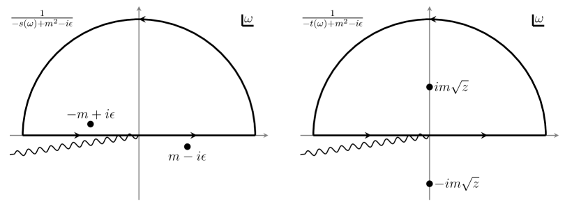
Figure 1: The analytic structure of the integral (3.19) for the tree-level exchange four-point function $f_{12\leftrightarrow 34}(z)$. Left: the $s$-channel contribution. Right: the $t$-channel contribution.

Let us return to the scalar theory considered in Section 3.1. The tree-level amplitude with massless external scalar particles exchanging a massive scalar is

$$\mathcal{T}(s,t)={g^{2}\over-s+m^{2}-i\epsilon}+{g^{2}\over-t+m^{2}-i\epsilon}+{g^{2}\over-u+m^{2}-i\epsilon}\,.$$ (3.26)

The massive scalar exchange amplitude is in some sense simpler than other tree-level amplitudes, for example the contact four-point or the massless exchange amplitudes. Indeed, the latter two suffer from either the UV or IR divergence for positive $\Delta_{\phi}$ in the change of basis integral (3.17). On the other hand, for the massive exchange amplitude, the mass $m$ of the intermediate particle provides an IR cut-off so that there is range of $\Delta_{\phi}$ where the amplitude in the conformal basis is well-defined. In fact, for sufficiently positive $\Delta_{\phi}$, there is a good physical reason for the divergence of the contact four-point and the massless exchange amplitudes in the conformal basis: they are exactly the bulk point singularity in $AdS_{3}/CFT_{2}$ of the corresponding Witten diagrams. We will come back to this point in Section 5.

Let us start with the $12\leftrightarrow 34$ channel where we take particles 1 and 2 to be incoming while 3 and 4 to be outgoing. Assuming $3/4<\text{Re}\,\Delta_{\phi}<5/4$, this amplitude (3.26) satisfies the fall-off condition (3.20), we can directly apply the residue formula (3.21) to obtain the amplitude in the $12\leftrightarrow 34$ channel:

$$f_{12\leftrightarrow 34}(z)=\mathcal{N}_{\Delta_{\phi}}\,{z\over\sqrt{z-1}}\left[\,e^{i\pi\alpha}+z^{\alpha}+\left({z\over z-1}\right)^{\alpha}\,\right]\,,~{}~{}~{}z>1\,,$$ (3.27)

where $\mathcal{N}_{\Delta_{\phi}}=g^{2}{\pi m^{4\Delta_{\phi}-5}\over 2^{4\Delta_{\phi}}\cos(2\pi\Delta_{\phi})}$ and

$$\alpha\equiv 2\Delta_{\phi}-\frac{3}{2}\,.$$ (3.28)

Similarly, in the $13\leftrightarrow 24$ channel, the four-point function is given by

$$f_{13\leftrightarrow 24}(z)=\mathcal{N}_{\Delta_{\phi}}\,{z\over\sqrt{1-z}}\left[\,1+e^{i\pi\alpha}z^{\alpha}+\left({z\over 1-z}\right)^{\alpha}\,\right]\,,~{}~{}0<z<1\,.$$ (3.29)

Finally in the $14\leftrightarrow 23$ channel, the four-point function is given by

$$f_{14\leftrightarrow 23}(z)=\mathcal{N}_{\Delta_{\phi}}\,{(-z)\over\sqrt{1-z}}\left[\,1+(-z)^{\alpha}+e^{i\pi\alpha}\left({-z\over 1-z}\right)^{\alpha}\,\right]\,,~{}~{}z<0\,.$$ (3.30)

Even though the change of basis integral only converges for $3/4<\text{Re}\,\Delta_{\phi}<5/4$, we can analytically continue the final expression to all complex $\Delta_{\phi}$ except for $\Delta_{\phi}\in\frac{1}{4}+\mathbb{Z}$.

One feature of these correlators is that they are complex even if we assume $\Delta_{\phi}$ to be real. This is of course expected because the amplitude is already complex in momentum space because of the $i\epsilon$ prescription. It follows that the imaginary part of these correlators should obey the optical theorem in the conformal basis, which we will discuss in Section 4.

4 Optical Theorem and Conformal Block Decomposition

In this section we translate the optical theorem into the conformal basis. In the case of the tree-level exchange amplitude, the optical theorem takes the form of a conformal block decomposition on the principal continuous series, with coefficients being the three-point amplitude in the conformal basis. We then verify this explicitly in a scalar theory in (2+1) dimensions.

4.1 Conformal Optical Theorem

Let us start with the simplest example of a tree-level massive scalar exchange amplitude $\mathcal{T}(s,t)$ in (3.26) in $\mathbb{R}^{1,d+1}$. The optical theorem relates the imaginary part of the four-point amplitudes to the product of two three-point amplitudes

$$2\,\text{Im}\,\mathcal{A}_{k_{1},k_{2}\rightarrow k_{3},k_{4}}=\pi\int{d^{d+1}\vec{p}\over\sqrt{\vec{p}^{2}+m^{2}}}\mathcal{A}_{k_{1},k_{2}\rightarrow p}\mathcal{A}_{k_{3},k_{4}\rightarrow p}\,.$$ (4.1)

where $\mathcal{A}_{k_{1},k_{2}\rightarrow k_{3},k_{4}}=\mathcal{T}(s,t)\delta^{(d+2)}(k_{1}+k_{2}-k_{3}-k_{4})$ and $\mathcal{A}_{k_{1},k_{2}\rightarrow p}=g\delta^{(d+2)}(k_{1}+k_{2}-p)$. Note that this simplest optical theorem follows from the identity:

$$\text{Im}\frac{1}{-s+m^{2}-i\epsilon}=\pi\delta(s-m^{2})\,.$$ (4.2)

Since we take particles 1 and 2 to be incoming while 3 and 4 to be outgoing, only the $s$-channel can go on-shell and contribute to the imaginary part of the amplitude.

To go to the conformal basis, we use the following orthogonality condition of the AdS bulk-to-boundary propagator [29] (see also [4]):

$$\int^{\infty}_{-\infty}d\nu\mu(\nu)\int d^{d}\vec{x}\,G_{\frac{d}{2}+i\nu}(\hat{p}_{1};\vec{x})G_{\frac{d}{2}-i\nu}(\hat{p}_{2};\vec{x})=(\hat{p}_{1})^{0}\,\delta^{(d+1)}(\hat{p}_{1}-\hat{p}_{2})\,,$$ (4.3)

where $\hat{p}_{i}$ are unit timelike vectors in $\mathbb{R}^{1,d+1}$ and the right-hand side is the $SO(1,d+1)$ invariant delta-function. The measure $\mu(\nu)$ is

$$\mu(\nu)=\frac{\Gamma\left(\frac{d}{2}+i\nu\right)\Gamma\left(\frac{d}{2}-i\nu\right)}{4\pi^{d+1}\Gamma(i\nu)\Gamma(-i\nu)}\,.$$ (4.4)

We can then insert $1=\int{d^{d+1}\hat{\ell}\over\hat{\ell}^{0}}\hat{\ell}^{0}\,\delta^{(d+1)}(\hat{\ell}-\hat{p})$ into the right-hand side of (4.1) and use (4.3) to obtain

$$2\,\text{Im}\,\mathcal{A}_{k_{1},k_{2}\rightarrow k_{3},k_{4}}$$ (4.5)

$$= \pi m^{d}\int^{\infty}_{-\infty}d\nu\mu(\nu)\int d^{d}\vec{x}\,\int\frac{d^{d+1}\hat{p}}{\hat{p}^{0}}\mathcal{A}_{k_{1},k_{2}\rightarrow p}G_{\frac{d}{2}+i\nu}(\hat{p};\vec{x})\int\frac{d^{d+1}\hat{\ell}}{\hat{\ell}^{0}}\mathcal{A}_{k_{3},k_{4}\rightarrow\ell}G_{\frac{d}{2}-i\nu}(\hat{\ell};\vec{x})\,.$$

Now we perform the change of basis integral (2.10) on the external particles $k_{1},\cdots,k_{4}$. In the conformal basis, the optical theorem is then translated into

$$2\,\text{Im}\,\widetilde{\mathcal{A}}_{4}(\Delta_{i},\vec{x}_{i})$$ (4.6)

$$=\pi m^{d}\int^{\infty}_{-\infty}d\nu\mu(\nu)\int d^{d}\vec{x}\,\widetilde{\mathcal{A}}_{3}\left(\Delta_{1},\Delta_{2},{d\over 2}+i\nu;\vec{x}_{1},\vec{x}_{2},\vec{x}\right)\widetilde{\mathcal{A}}_{3}\left({d\over 2}-i\nu,\Delta_{3},\Delta_{4},;\vec{x},\vec{x}_{3},\vec{x}_{4}\right)\,,$$

where we have assigned conformal dimension $\Delta_{i}$ to the $i$-th external particle. The optical theorem can be further simplified by using the explicit positions dependence of the three-point functions:

$$\widetilde{\mathcal{A}}_{3}(\Delta_{i},\vec{x}_{i})={C(\Delta_{1},\Delta_{2};\Delta_{3})\over|\vec{x}_{12}|^{\Delta_{1}+\Delta_{2}-\Delta_{3}}|\vec{x}_{13}|^{\Delta_{1}+\Delta_{3}-\Delta_{2}}|\vec{x}_{23}|^{\Delta_{2}+\Delta_{3}-\Delta_{1}}}\,.$$ (4.7)

The integral over $\vec{x}$ gives the shadow representation of the conformal partial wave $\Psi_{\Delta}(z,\bar{z})$ [24, 25, 26, 27]:

$$\frac{\Psi_{\Delta}(z,\bar{z})}{|\vec{x}_{12}|^{\Delta_{1}+\Delta_{2}}|\vec{x}_{34}|^{\Delta_{3}+\Delta_{4}}}\left|\frac{\vec{x}_{24}}{\vec{x}_{14}}\right|^{\Delta_{12}}\left|\frac{\vec{x}_{14}}{\vec{x}_{13}}\right|^{\Delta_{34}}$$ (4.8)

$$= \frac{1}{2}\int d^{d}\vec{w}\frac{|\vec{x}_{12}|^{\Delta-\Delta_{1}-\Delta_{2}}|\vec{x}_{34}|^{d-\Delta-\Delta_{3}-\Delta_{4}}}{|\vec{w}-\vec{x}_{1}|^{\Delta_{12}+\Delta}|\vec{w}-\vec{x}_{2}|^{\Delta_{21}+\Delta}|\vec{w}-\vec{x}_{3}|^{\Delta_{34}+d-\Delta}|\vec{w}-\vec{x}_{4}|^{\Delta_{43}+d-\Delta}}\,,$$

where $\vec{x}_{ij}=\vec{x}_{i}-\vec{x}_{j}$ and $\Delta_{ij}=\Delta_{i}-\Delta_{j}$. $z,\bar{z}$ are the cross ratios:

$$\begin{gathered}z\bar{z}=\frac{|\vec{x}_{12}|^{2}|\vec{x}_{34}|^{2}}{|\vec{x}_{13}|^{2}|\vec{x}_{24}|^{2}}\,,\quad(1-z)(1-\bar{z})=\frac{|\vec{x}_{14}|^{2}|\vec{x}_{23}|^{2}}{|\vec{x}_{13}|^{2}|\vec{x}_{24}|^{2}}\,.\end{gathered}$$ (4.9)

$\Psi_{\Delta}(z,\bar{z})$ is an eigenfunction of the conformal Casimir operator that is shadow symmetric, i.e. $\Psi_{\Delta}=\Psi_{d-\Delta}$. It is related to the scalar conformal blocks $G_{\Delta}^{(\ell=0)}(z,\bar{z})$ with intermediate scalar primaries as [26],

$$\Psi_{\Delta}(z,\bar{z})=\frac{c_{\Delta}G_{\Delta}^{(\ell=0)}(z,\bar{z})+c_{d-\Delta}G^{(\ell=0)}_{d-\Delta}(z,\bar{z})}{2\Gamma\left(\frac{\Delta+\Delta_{21}}{2}\right)\Gamma\left(\frac{\Delta-\Delta_{21}}{2}\right)\Gamma\left(\frac{d-\Delta+\Delta_{34}}{2}\right)\Gamma\left(\frac{d-\Delta-\Delta_{34}}{2}\right)}\,,$$ (4.10)

where the coefficient $c_{\Delta}$ is

$$c_{\Delta}=\pi^{d/2}\frac{\Gamma\left(\frac{d}{2}-\Delta\right)\Gamma\left(\frac{\Delta+\Delta_{34}}{2}\right)\Gamma\left(\frac{\Delta-\Delta_{34}}{2}\right)\Gamma\left(\frac{\Delta+\Delta_{21}}{2}\right)\Gamma\left(\frac{\Delta-\Delta_{21}}{2}\right)}{\Gamma\left(\Delta\right)}\,.$$ (4.11)

If we write the four-point function as

$$\widetilde{\mathcal{A}}_{4}(\Delta_{i},\vec{x}_{i})={|\vec{x}_{12}|^{\Delta_{1}+\Delta_{2}}|\vec{x}_{34}|^{\Delta_{3}+\Delta_{4}}}\left|\frac{\vec{x}_{24}}{\vec{x}_{14}}\right|^{\Delta_{12}}\left|\frac{\vec{x}_{14}}{\vec{x}_{13}}\right|^{\Delta_{34}}f(z,\bar{z})\,,$$ (4.12)

then the optical theorem gives the conformal block decomposition for the imaginary part of $f(z,\bar{z})$ on the principal continuous series

$$\boxed{\,\text{Im}f(z,\bar{z})=\pi m^{d}\int^{\infty}_{-\infty}d\nu\mu(\nu)C\left(\Delta_{1},\Delta_{2};\frac{d}{2}+i\nu\right)C\left(\Delta_{3},\Delta_{4};\frac{d}{2}-i\nu\right)\Psi_{\frac{d}{2}+i\nu}(z,\bar{z})\,,}$$ (4.13)

with coefficient being the three-point amplitude written in the conformal basis (4.7).

The derivation can be extended to the general optical theorem straightforwardly,

$$2\text{Im}\mathcal{T}_{\{p\}\rightarrow\{q\}}=\sum_{\{k\}}\prod_{j}\left(\int\frac{d^{d+1}\vec{k}_{j}}{(2\pi)^{d+1}2k^{0}_{j}}\right)\mathcal{T}_{\{p\}\rightarrow\{k\}}\mathcal{T}_{\{q\}\rightarrow\{k\}}(2\pi)^{d+2}\delta^{(d+2)}\left(\sum p-\sum k\right)\,,$$ (4.14)

where $p,q,k$ are the sets of momenta of the initial, final and intermediate particles. The sum in $\{k\}$ is over all possible intermediate particle states. The general optical theorem when translated into the conformal basis is

$$2\text{Im}\widetilde{\mathcal{A}}(\Delta_{I},\Delta_{F},\vec{x}_{i})= (2\pi)^{d+2}\sum_{\{k\}}\prod_{j}\left(\frac{m_{j}^{d}}{2(2\pi)^{d+1}}\int^{\infty}_{-\infty}d\nu_{j}\mu(\nu_{j})\int d^{d}\vec{w}_{j}\right)$$ (4.15)

$$~{}~{}~{}~{}~{}~{}~{}~{}~{}~{}\times\widetilde{\mathcal{A}}\left(\Delta_{I},{d\over 2}+i\nu_{j};\vec{x}_{I},\vec{w}_{j}\right)\widetilde{\mathcal{A}}\left({d\over 2}-i\nu_{j},\Delta_{F};\vec{w}_{j},\vec{x}_{F}\right)\,.$$

where $I$ and $F$ are the subscripts for the conformal dimensions and the positions of the initial and final conformal primary wave functions, respectively.

4.2 Example: Tree-Level Exchange Amplitude

We now explicitly show that, in the case of the exchange diagram in (2+1) dimensions, the conformal block decomposition of the four-point function in (3.27) reproduces the three-point function coefficient in (3.7). In one dimension, the conformal partial wave $\Psi_{\frac{d}{2}+i\nu}(z)$, defined for $z>0$, has been worked out in [56] (see also [21])

$$\Psi_{\Delta}(z)=\begin{dcases}\frac{\tan\pi\Delta}{2\tan\frac{\pi\Delta}{2}}\frac{\Gamma(\Delta)^{2}}{\Gamma(2\Delta)}z^{\Delta}{}_{2}F_{1}(\Delta,\Delta;2\Delta;z)+(\Delta\leftrightarrow 1-\Delta),\quad&0<z<1\,,\\ {\Gamma(\frac{1}{2}-\frac{\Delta}{2})\Gamma(\frac{\Delta}{2})\over\sqrt{\pi}}\,_{2}F_{1}\left(\frac{\Delta}{2},\frac{1}{2}-\frac{\Delta}{2};\frac{1}{2};{(2-z)^{2}\over z^{2}}\right),\quad&1<z<2\,,\\ \Psi_{\Delta}\left(\frac{z}{z-1}\right),\quad&2<z\,.\end{dcases}$$ (4.16)

$\Psi_{\Delta}(z)$’s on the principal discrete series $\Delta\in 2\mathbb{N}$ together with the principal continuous series $\Delta\in\frac{1}{2}+i\mathbb{R}_{\geq 0}$ form an orthogonal basis for the space of functions with the following boundary conditions (1) $f(z)=f(\frac{z}{z-1})$ for $z\in(1,\infty)$ which in particular implies $f^{\prime}(2)=0$, and (2) $f(z)$ vanishes no slower than $z^{1/2}$ as $z\rightarrow 0$. The inner product on this space of functions is

$$\langle g,f\rangle=\int^{2}_{0}\frac{dz}{z^{2}}g^{*}(z)f(z)=\left(\int^{1}_{0}+\frac{1}{2}\int_{1}^{\infty}\right)\frac{dz}{z^{2}}g^{*}(z)f(z)\,,$$ (4.17)

where the integral between $(1,2)$ is replaced by an integral between $(1,\infty)$ using the symmetry $f(z)=f(\frac{z}{z-1})$. The inner products of $\Psi_{\Delta}$ are

$$\langle\Psi_{\Delta},\Psi_{\Delta^{\prime}}\rangle =\frac{\pi^{2}}{4\Delta-2}\delta_{\Delta,\Delta^{\prime}},~{}~{}~{}~{}~{}~{}~{}~{}~{}~{}~{}~{}~{}~{}~{}~{}~{}~{}\,\Delta,\Delta^{\prime}\in 2\mathbb{N}$$ (4.18)

$$\langle\Psi_{\Delta},\Psi_{\Delta^{\prime}}\rangle =\frac{\pi^{2}\tan\pi\Delta}{2\Delta-1}\delta(\Delta-\Delta^{\prime}),\quad~{}~{}~{}~{}~{}\Delta,\Delta^{\prime}\in\frac{1}{2}+i\mathbb{R}_{\geq 0}\,.\,$$

Let us decompose the four-point function $f_{12\leftrightarrow 34}(z)$ in (3.27) on this basis. The imaginary part of $f_{12\leftrightarrow 34}$ can be written as

$$2\text{Im}{f}_{12\leftrightarrow 34}(z)=2\mathcal{N}_{\Delta_{\phi}}\sin\left(2\pi\Delta_{\phi}-\frac{3\pi}{2}\right)F(z),\quad F(z)=\begin{dcases}\frac{z}{\sqrt{z-1}},&1<z\\ 0,&0<z<1\,.\end{dcases}$$ (4.19)

Recall that the real cross ratio $z$ in $12\leftrightarrow 34$ channel is constrained by the flat space kinematics to be $z>1$. This function satisfies the two boundary conditions: $F(z)=F(\frac{z}{z-1})$ for $z\in(1,\infty)$ and $\lim_{z\rightarrow 0}F^{\prime}(z)/z^{1/2}=0$. Thus it can be expanded on the basis with the coefficients proportional to the inner product

$$\langle F,\Psi_{\Delta}\rangle=\frac{1}{2}\int^{\infty}_{1}\frac{dz}{z^{2}}\frac{z}{\sqrt{z-1}}\Psi_{\Delta}(z)=\frac{\pi^{3}}{\sin(\pi\Delta)\Gamma(\frac{2-\Delta}{2})^{2}\Gamma(\frac{\Delta+1}{2})^{2}}\,.$$ (4.20)

Since the inner products vanishes on the principal discrete series $h\in 2\mathbb{N}$, $F(z)$ can be expanded just on the principal continuous series,

$$F(z)=\int^{\frac{1}{2}+i\infty}_{\frac{1}{2}-i\infty}\frac{d\Delta}{2\pi i}\frac{2\Delta-1}{\pi\tan(\pi\Delta)}\frac{\pi^{3}}{\sin(\pi\Delta)\Gamma(\frac{2-\Delta}{2})^{2}\Gamma(\frac{\Delta+1}{2})^{2}}\Psi_{\Delta}(z)\,,$$ (4.21)

where we have used the symmetry $\Delta\leftrightarrow 1-\Delta$ of the integrand to extend the integration from $\frac{1}{2}+i\mathbb{R}_{\geq 0}$ to $\frac{1}{2}+i\mathbb{R}$. The coefficient of the above decomposition can be written in terms of the three-point function coefficient (3.7) as

$$\text{Im}f_{12\leftrightarrow 34}(z) =\pi m\int^{\infty}_{-\infty}d\nu\mu(\nu)C\left(\Delta_{1},\Delta_{2};\frac{d}{2}+i\nu\right)C\left(\Delta_{1},\Delta_{2};\frac{d}{2}-i\nu\right)\Psi_{\frac{d}{2}+i\nu}(z,\bar{z})\,,$$ (4.22)

where $C(\Delta_{\phi},\Delta_{\phi};\Delta)=g\frac{m^{2\Delta_{\phi}-3}}{2^{2\Delta_{\phi}}}\frac{\Gamma\left(\Delta/2\right)^{2}}{\Gamma(\Delta)}$. Hence we have checked the conformal block decomposition (4.13) in the (2+1)-dimensional scalar theory with cubic coupling.

5 The Bulk Point Singularity in AdS/CFT

In this section we discuss the relation between the massless conformal basis in $\mathbb{R}^{1,d+1}$ and the bulk point singularity in $AdS_{d+2}/CFT_{d+1}$ in Lorentzian signature. In particular we argue that scalar exchange amplitudes in the conformal basis discussed in Section 3.4 arise from approaching the bulk point singularity at the same time scaling the intermediate conformal dimension to infinite in the exchange Witten diagram.

Let us begin with a general review on the bulk point singularity in $AdS/CFT$ and its relation to the flat space limit [41, 42, 36, 37, 28, 38, 39]. Consider $AdS_{d+2}$ embedded in $\mathbb{R}^{2,d+1}$ as the locus $Y^{I}Y_{I}=-R^{2}$, where $R$ is the AdS radius. Here we use $Y^{I}$ with $I=-1,0,1,\cdots,d+1$ as the flat coordinates of the embedding space $\mathbb{R}^{2,d+1}$ and the index $I$ is raised and lowered by the flat metric $\eta_{IJ}=\text{diag}(-1,-1,+1,\cdots,+1)$. On the other hand, a point on the boundary of $AdS_{d+2}$ is represented by a null ray $P^{I}\sim\lambda P^{I}$ with $P^{I}P_{I}=0$.

Consider an $n$-point Witten diagram with boundary operators located at $P^{I}_{a}$, $a=1,\cdots,n$. We will restrict ourselves to the case $n=d+3$ so that in this case the vertex of the Landau diagram is only a point in $AdS_{d+2}$. The conditions for the bulk point singularity are that there exists a bulk point $Y_{0}$ such that

1. $Y_{0}$ is lightlike separated from all the boundary points $P_{a}$,

   $$\eta_{IJ}\,Y^{I}_{0}P^{J}_{a}=0\,,~{}~{}~{}~{}\forall\,a=1,2,\cdots,n\,.$$ (5.1)

2. There exist $n$ “frequencies” $\omega_{a}>0$ such that the momentum is conserved at $Y_{0}$:

   $$\sum_{a=1}^{n}\omega_{a}P^{I}_{a}=0\,.$$ (5.2)

In general such a bulk point $Y_{0}$ does not exist for generic boundary points $P_{a}$. In other words, the bulk point singularity only arises when we place the boundary points at some specific configuration. For example, in the case of four-point functions, the second condition (5.2) implies that the 4$\times 4$ matrix $P_{a}\cdot P_{b}$ has a zero eigenvector $\omega_{a}$, and hence it has vanishing determinant. This in turns implies the cross ratios are real at the bulk point singularity configuration, i.e. $z=\bar{z}$.

The bulk point singularity configuration is related to the flat space scattering kinematics in $\mathbb{R}^{1,d+1}$. Let us take our reference bulk point to be at $Y_{0}=(R,0,\cdots,0).$ Then the first condition (5.1) constrains the boundary points $P^{I}_{a}$ to be

$$P^{I}_{a}=(0,\pm q^{\mu}_{a})\,,$$ (5.3)

where $q^{\mu}_{a}$ is a null ray in $\mathbb{R}^{1,d+1}$ with $\mu=0,1,\cdots,d+1$. Here we take the time component of $q^{\mu}$ to be positive, so that the plus/minus sign above corresponds to a null vector in the future/past lightcone of $\mathbb{R}^{1,d+1}$ in the embedding space, respectively. In other words, the boundary points are restricted to two constant time slices in $AdS_{d+2}$ at the bulk point singularity configuration (see Figure 2). The null vectors $q^{\mu}_{a}$ are later identified as the directions of null momenta in the flat space scattering process. Now the second condition (5.2) states that there exists $n$ frequencies $\omega_{a}$ such that the flat space momentum conservation $\sum_{a}\pm\omega_{a}q^{\mu}_{a}=0$ holds true. In the case of the bulk point singularity for four-point functions, the real cross ratio $z=\bar{z}$ parametrizes the scattering angle.

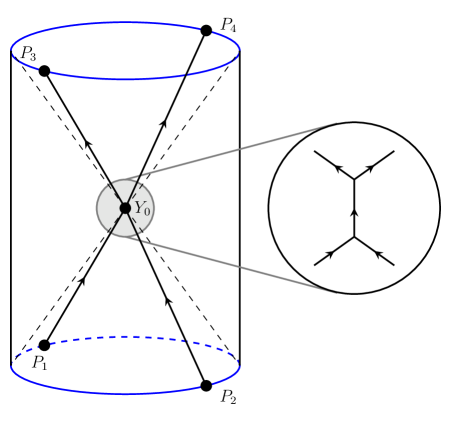
Figure 2: The bulk point singularity in $AdS_{3}$. At the bulk point singularity configuration for a four-point function in $AdS_{3}/CFT_{2}$, the boundary points are restricted to two constant time slices in $AdS_{3}$, which are the future and past celestial circles (shown in blue) in the flat space limit to $\mathbb{R}^{1,2}$. The contribution to the Witten diagram is dominated by the integral around the bulk point $Y_{0}$, which can then be approximated by the flat space scattering process in the massless conformal basis.

We now argue that perturbative scattering amplitudes in the massless conformal basis in $\mathbb{R}^{1,d+1}$ can be embedded into the $AdS_{d+2}$ Witten diagram with the same interaction at the bulk point singularity. The scalar bulk-to-boundary propagator in $AdS_{d+2}$ between a bulk point $Y$ and a boundary point $P$ with conformal dimension $\Delta_{\phi}$ is

$$G_{\Delta_{\phi}}(Y,P)={\mathcal{C}_{\Delta}\over R^{d\over 2}}{1\over(-2P\cdot Y/R+i\epsilon)^{\Delta_{\phi}}}\,,$$ (5.4)

where $\mathcal{C}_{\Delta}=\Gamma(\Delta)/(2\pi^{d+1\over 2}\Gamma(\Delta-\frac{d-1}{2}))$. At the bulk point singularity configuration, from (5.3), the null ray $P_{a}^{I}$ in $\mathbb{R}^{2,d+1}$ is restricted to a null ray $q_{a}^{\mu}$ in $\mathbb{R}^{1,d+1}$. Furthermore, the contribution to the Witten diagram receives dominant contributions from around $Y_{0}$, and we can approximate the bulk point integral in $Y$ by a flat space integral in $X^{\mu}\in\mathbb{R}^{1,d+1}$ around $Y_{0}$. In this limit, the $AdS_{d+2}$ bulk-to-boundary propagator becomes proportional to the massless conformal primary wavefunction $\varphi^{\pm}_{\Delta_{\phi}}$ (2.4) in $\mathbb{R}^{1,d+1}$:

$$G_{\Delta_{\phi}}(Y,P)\,\underset{\text{bulk point singularity}}{\longrightarrow}\,\varphi_{\Delta_{\phi}}^{\pm}(X,q)\,.$$ (5.5)

Whether the corresponding conformal primary wavefunction is incoming or outgoing is determined by which of the past and future time slices the boundary point $P^{I}_{a}$ is located at (i.e. the sign in (5.3)).

Following the same argument in [36, 39], let us see how this works explicitly for the tree-level scalar exchange Witten diagram in $AdS_{3}/CFT_{2}$. We will focus only on the $s$-channel diagram, while the other two follow identically.

The scalar bulk-to-bulk propagator with intermediate conformal dimension $\Delta$ is (see, for example, [57])

$$\Pi_{\Delta}(Y_{1},Y_{2})={1\over 2\pi R}{e^{-\Delta\sigma}\over 1-e^{-2\sigma}}\,,$$ (5.6)

where $\sigma$ is the geodesic distance between $Y_{1},Y_{2}$:

$$\sigma(Y_{1},Y_{2})=\log\left({1+\sqrt{1-\xi^{2}+i\epsilon}\over\xi}\right)\,,~{}~{}~{}~{}~{}~{}\xi=-{R^{2}\over Y_{1}\cdot Y_{2}}\,.$$ (5.7)

The $s$-channel tree-level scalar Witten diagram with internal dimension $\Delta$ and identical external operator dimension $\Delta_{\phi}$ is

$$I_{4} =g^{2}\int_{AdS_{3}}dY_{1}\int_{AdS_{3}}dY_{2}\,G_{\Delta_{\phi}}(Y,P_{1})G_{\Delta_{\phi}}(Y,P_{2})\Pi_{\Delta}(Y_{1},Y_{2})G_{\Delta_{\phi}}(Y,P_{3})G_{\Delta_{\phi}}(Y,P_{4})$$

$$=g^{2}\left({e^{-i\pi\Delta_{\phi}/2}\over 2^{\Delta_{\phi}+1}\pi R^{1/2}\Gamma(\Delta_{\phi})}\right)^{4}\int_{AdS_{3}}dY_{1}\int_{AdS_{3}}dY_{2}\,$$

$$\times\left(\prod_{a=1}^{4}\int_{0}^{\infty}d\omega_{a}\omega_{a}^{\Delta_{\phi}-1}\right)e^{-iY_{1}\cdot(\omega_{1}P_{1}+\omega_{2}P_{2})-iY_{2}\cdot(\omega_{3}P_{3}+\omega_{4}P_{4})-\epsilon\sum_{a}\omega_{a}}\Pi_{\Delta}(Y_{1},Y_{2})\,.$$ (5.8)

Let us now approach the bulk point singularity by tuning the boundary points to be close to the configuration (5.1) and (5.2). We will choose $P_{1,2}$ to be $(0,-q_{1,2}^{\mu})$ and while $P_{3,4}$ to be $(\delta,q_{3,4}^{\mu})$. If we also choose $q_{a}^{\mu}$ to be such that (5.2) is obeyed, then we reach the bulk point singularity configuration as $\delta\to 0$. In this limit we expect the contribution of the integral in (5) to be dominated by $Y_{1},Y_{2}$ close to $Y_{0}=(R,0,0,0)$, which can then be approximated by integrals over $\mathbb{R}^{1,d}$. To be more explicit, near $Y_{0}$, we can parametrize a bulk point $Y$ as $Y^{I}\simeq(R+{X^{\mu}X_{\mu}\over 2R},X^{\mu})$, where every component of $X^{\mu}$ is much less that $R$. Equivalently, we can take $R\to\infty$ and allow $X^{\mu}\in\mathbb{R}^{1,2}$ to be integrated to infinity in (5).

In this limit, the Witten diagram becomes

$$I_{4} \simeq g^{2}\left({e^{-i\pi\Delta_{\phi}/2}\over 2^{\Delta_{\phi}+1}\pi R^{1/2}\Gamma(\Delta_{\phi})}\right)^{4}\left(\prod_{a=1}^{4}\int_{0}^{\infty}d\omega_{a}\omega_{a}^{\Delta_{\phi}-1}\right)$$

$$\times\int_{\mathbb{R}^{1,2}}d^{3}X_{1}\int_{\mathbb{R}^{1,2}}d^{3}X_{2}e^{iX_{1}\cdot(\omega_{1}q_{1}+\omega_{2}q_{2})-iX_{2}\cdot(\omega_{3}q_{3}+\omega_{4}q_{4})+iR(\omega_{3}+\omega_{4})\delta-\epsilon\sum_{a}\omega_{a}}\Pi_{\Delta}(Y_{1},Y_{2})\,.$$ (5.9)

If we keep the intermediate conformal dimension $\Delta$ finite as taking $R\to\infty$, then the bulk-to-bulk propagator $\Pi_{\Delta}(Y_{1},Y_{2})$ is approximated by the massless Feynman scalar propagator in $\mathbb{R}^{1,2}$, i.e. $\Pi_{\Delta}\simeq{1\over 4\pi}{1\over\sqrt{(X_{1}-X_{2})^{2}+i\epsilon}}$. The $\omega_{a}$ integrals then give rise to a singularity $1/\delta^{4\Delta_{\phi}-5}$ as $\delta\to 0$. This is indeed the singularity computed in [36] using the explicit expression for $I_{4}$ in terms of the $D$-function for special values of $\Delta$. In the strict $\delta=0$ case, the above integral is identical to the massless scalar exchange amplitude in $\mathbb{R}^{1,2}$ written in the massless conformal basis. As discussed in Section 3.4, the change of basis integral (3.17) to the conformal basis suffers from an UV divergence (for sufficiently positive $\Delta_{\phi}$). Now we have an alternative understanding of this singularity: it comes from the bulk point singularity of the same interaction in $AdS_{3}$.

If instead we scale the intermediate conformal dimension $\Delta$ to infinite at the same rate as sending $R\to\infty$, while holding the ratio $m\equiv\Delta/R$ fixed, then the $AdS_{3}$ bulk-to-bulk propagator is approximated by the massive scalar Feynman propagator in $\mathbb{R}^{1,2}$:

$$\Pi_{\Delta}(Y_{1},Y_{2})\simeq{1\over 4\pi}{1\over\sqrt{(X_{1}-X_{2})^{2}+i\epsilon}}e^{-m\sqrt{(X_{1}-X_{2})^{2}+i\epsilon}}\,.$$ (5.10)

The second line of (5) is nothing but the Fourier transform from position space to momentum space for the flat space amplitude ${1\over s-m^{2}+i\epsilon}\delta^{(3)}(\sum_{a}k_{a})$ with null momenta $k_{a}=\pm\omega_{a}q_{a}$. Thus the scalar exchange Witten diagram (5) in this double scaling limit exactly reproduces the same Feynman diagram in $\mathbb{R}^{1,2}$ written in the massless conformal basis, which we computed in Section 3.4:

$$I_{4}\propto\left(\prod_{a=1}^{4}\int_{0}^{\infty}d\omega_{a}\omega_{a}^{\Delta_{\phi}-1}\right){\delta^{(3)}(\omega_{1}q_{1}^{\mu}+\omega_{2}q_{2}^{\mu}-\omega_{3}q_{3}^{\mu}-\omega_{4}q_{4}^{\mu})\over s-m^{2}+i\epsilon}\,,~{}~{}~{}~{}s=-(\omega_{1}q_{1}+\omega_{2}q_{2})^{2}\,.$$ (5.11)

The infinite intermediate conformal dimension $\Delta$ limit regulates the $\omega_{a}$ integrals near the would-be bulk point singularity, while it damps the contribution from the $AdS$ integrals away from the point $Y_{0}$.

From this perspective, the (2+1)-dimensional flat space amplitudes written in the massless conformal basis $f(z)$ should perhaps be interpreted as two-dimensional Lorentzian conformal correlators, restricted to the bulk point singularity configuration $z=\bar{z}$. In Appendix A, we present a $2d$ Euclidean correlator whose Lorentzian versions, when restricted to $z=\bar{z}$, are exactly the (2+1)-dimensional tree-level exchange amplitudes in the conformal basis $f_{12\leftrightarrow 34}(z),f_{13\leftrightarrow 24}(z),f_{14\leftrightarrow 23}(z)$. We leave the physical origin of this $2d$ Euclidean correlator for future investigation.

Appendix A Two-Dimensional Crossing Symmetric Four-Point Functions with Positive Block Decompositions

In this appendix we present a $2d$ Euclidean correlator $f^{2d}(z,\bar{z})$ whose Lorentzian versions, obtained via different analytic continuations in $z,\bar{z}$, are the (2+1)-dimensional amplitudes from three crossing channels $f_{12\leftrightarrow 34}(z),f_{13\leftrightarrow 24}(z),f_{14\leftrightarrow 23}(z)$. We checked to high orders that this $2d$ correlator admits a positive $SL(2,\mathbb{C})$ block decomposition. For a special value of the external conformal dimension $\Delta_{\phi}$, $f^{2d}(z,\bar{z})$ reduces to the four-point function in the $2d$ free boson theory.

A.1 A Two-Dimensional Extension

We now present an observation that in the example of tree-level exchange diagram, the correlators in the three crossing channels $f_{12\leftrightarrow 34},f_{13\leftrightarrow 24},f_{14\leftrightarrow 23}$ are restrictions of different analytic continuations of a single 2$d$ Euclidean correlator $f^{2d}(z,\bar{z})$.

Let the two cross ratios $z,\bar{z}$ of a $2d$ four-point function bedefined as

$$z={z_{12}z_{34}\over z_{13}z_{24}}\,,~{}~{}~{}~{}\bar{z}={\bar{z}_{12}\bar{z}_{34}\over\bar{z}_{13}\bar{z}_{24}}\,.$$ (A.1)

In the Euclidean signature, $z,\bar{z}$ are complex conjugated to each other, i.e. $\bar{z}=z^{*}$. On the other hand, in the Lorentzian signature, $z,\bar{z}$ are two independent real variables. Starting from an Euclidean $2d$ four-point function, its Lorentzian version can be obtained by analytic continuing the cross ratios $z,\bar{z}$ independently. The precise analytic continuation depends on the time ordering between the four operators in the Lorentzian spacetime.

If we place operators 1 and 2 in the past while 3 and 4 in the future, this corresponds to the following analytic continuation in $z,\bar{z}$ (see, for example, [59, 39] for explanations of this analytic continuation):

$$12\to 34:~{}(z-1)\to e^{2\pi i}(z-1)\,,~{}~{}~{}~{}{1\over\bar{z}}\to e^{2\pi i}{1\over\bar{z}}\,.$$ (A.2)

If instead we want to have 1 and 3 in the past while 2 and 4 in the future, we should analytically continue the cross ratios as

$$13\to 24:~{}z\to e^{2\pi i}z\,,~{}~{}~{}~{}(\bar{z}-1)\to e^{2\pi i}(\bar{z}-1)\,.$$ (A.3)

In addition, due to the overall factor ${1\over|z_{12}|^{2\Delta_{\phi}}|z_{34}|^{2\Delta_{\phi}}}$, one needs to further multiply the four-point function $f(z,\bar{z})$ by $e^{-2\pi i\Delta_{\phi}}$. This is because $|z_{12}|^{2}$ crosses the lightcone in the analytic continuation. Finally, if we place 1 and 4 in the past, 2 and 3 in the future, we analytically continue the cross ratios as

$$14\to 23:~{}\frac{1}{z}\to e^{2\pi i}\frac{1}{z}\,,~{}~{}~{}~{}\bar{z}\to e^{2\pi i}\bar{z}\,.$$ (A.4)

In addition, we need to multiply the four-point function by a phase $e^{-2\pi i\Delta_{\phi}}$.

Now consider the following two-dimensional Euclidean four-point function

$${\mathcal{A}}(z,\bar{z})={1\over|z_{12}|^{2\Delta_{\phi}}|z_{34}|^{2\Delta_{\phi}}}f^{2d}(z,\bar{z})\,,$$ (A.5)

$$f^{2d}(z,\bar{z})=\mathcal{N}_{\Delta_{\phi}}e^{i\pi(2\Delta_{\phi}-\frac{1}{2})}{(z\bar{z})^{\frac{1}{2}}\over[(1-z)(1-\bar{z})]^{\frac{1}{4}}}\left[1+(z\bar{z})^{\Delta_{\phi}-\frac{3}{4}}+\left({z\bar{z}\over(1-z)(1-\bar{z})}\right)^{\Delta_{\phi}-\frac{3}{4}}\right]\,.$$ (A.6)

This $2d$ Euclidean correlator satisfies the crossing equation (A.9) and admits a positive $SL(2,\mathbb{C})$ block decomposition as discussed in the next subsection. If we first analytically continue $f^{2d}(z,\bar{z})$ to the Lorentzian regime as (A.2), (A.3), (A.4), and then restrict to $z=\bar{z}$, we exactly reproduce the (2+1)-dimensional tree-level exchange amplitudes $f_{12\leftrightarrow 34},f_{13\leftrightarrow 24},f_{14\leftrightarrow 23}$ (3.27), (3.29), (3.30) in three different crossing channels, respectively:

$$\begin{split}&f_{12\leftrightarrow 34}(z)=f^{2d}(z,\bar{z})\Big{|}_{(z-1)\to e^{2\pi i}(z-1),\frac{1}{\bar{z}}\to e^{2\pi i}{1\over\bar{z}}}\,\Big{|}_{z=\bar{z}}\,,\\ &f_{13\leftrightarrow 24}(z)=e^{-2\pi i\Delta_{\phi}}f^{2d}(z,\bar{z})\Big{|}_{z\to e^{2\pi i}z,(\bar{z}-1)\to e^{2\pi i}(\bar{z}-1)}\,\Big{|}_{z=\bar{z}}\,,\\ &f_{14\leftrightarrow 23}(z)=e^{-2\pi i\Delta_{\phi}}f^{2d}(z,\bar{z})\Big{|}_{\frac{1}{z}\to e^{2\pi i}\frac{1}{z},\bar{z}\to e^{2\pi i}\bar{z}}\,\Big{|}_{z=\bar{z}}\,,\end{split}$$ (A.7)

where the phase $e^{-2\pi i\Delta_{\phi}}$ comes from the prefactor ${1\over|z_{12}|^{2\Delta_{\phi}}|z_{34}|^{2\Delta_{\phi}}}$ in our definition of $\tilde{f}(z,\bar{z})$ in relation to the full four-point function. This implies that the one-dimensional four-point functions are restrictions of $f(z,\bar{z})$ to the Lorentzian configurations similar to Figure 2.

A.2 Positive Conformal Block Decompositions

In fact, the Euclidean $2d$ four-point function $f^{2d}(z,\bar{z})$ (A.5) belongs to a larger family of solutions to the crossing equation. In this section we provide numerical evidence that this family of crossing solutions have positive conformal block decompositions.

Let us consider a generalization of the $2d$ scalar four-point function (A.5) considered above:

$$f_{\Delta_{\phi},b}(z,\bar{z})={(z\bar{z})^{\Delta_{\phi}-\frac{b}{2}}\over((1-z)(1-\bar{z}))^{b\over 2}}\left[\,(z\bar{z})^{-\Delta_{\phi}+{3b\over 2}}+1+((1-z)(1-\bar{z}))^{-\Delta_{\phi}+{3b\over 2}}\,\right]\,.$$ (A.8)

This four-point function comes with a two-parameter family, labeled by the external operator dimension $\Delta_{\phi}$ (which will be taken to be positive in this appendix) and a real parameter $b$. The four-point function $f_{\Delta_{\phi},b}$ is crossing symmetric for all $\Delta_{\phi},b$:

$$f_{\Delta_{\phi},b}(z,\bar{z})=\left({z\bar{z}\over(1-z)(1-\bar{z})}\right)^{\Delta_{\phi}}f_{\Delta_{\phi},b}(1-z,1-\bar{z})=(z\bar{z})^{\Delta_{\phi}}f_{\Delta_{\phi},b}(1/z,1/\bar{z})\,.$$ (A.9)

For general $\Delta_{\phi}$ and $b$, the operator spectrum in the OPE channel $z,\bar{z}\to 0$ can be separated into towers of “single-trace” and the “double-trace” operators:

$$\begin{split}&\text{Single-trace}:\,~{}~{}\Delta=2b+\ell+4m\,,~{}~{}~{}~{}~{}~{}\,~{}~{}~{}~{}m\in\mathbb{Z}_{\geq 0}\,,\\ &\text{Double-trace}:~{}\Delta=2\Delta_{\phi}-b+\ell+2m\,,~{}~{}~{}m\in\mathbb{Z}_{\geq 0}\,,\end{split}$$ (A.10)

where $\ell\in 2\mathbb{Z}_{\geq 0}$ is the spin. We distinguish a double-trace operator from a single-trace one by the dependence of their conformal dimensions on $\Delta_{\phi}$. The conformal block expansion of the four-point function can be separated into single- and double-trace operators:

$$f_{\Delta_{\phi},b}(z,\bar{z})=\sum_{\begin{subarray}{c}\ell=0,\\ \text{even}\end{subarray}}^{\infty}\sum_{m=0}^{\infty}c_{\ell+4m,\ell}\,G_{2b+\ell+4m}^{(\ell)}(z,\bar{z})+\sum_{\begin{subarray}{c}\ell=0,\\ \text{even}\end{subarray}}^{\infty}\sum_{m=0}^{\infty}c^{d}_{\ell+2m,\ell}\,G_{2\Delta_{\phi}-b+\ell+2m}^{(\ell)}(z,\bar{z})\,,$$ (A.11)

where the $SL(2,\mathbb{C})$ block with identical external scalar primaries of dimension $\Delta_{\phi}$ and intermediate conformal dimension $\Delta$ and spin $\ell\geq 0$ is [60, 25, 61, 26]

$$G^{(\ell)}_{\Delta}(z,\bar{z})= {1\over 1+\delta_{\ell,0}}\Big{[}z^{\frac{1}{2}(\Delta+\ell)}\,\bar{z}^{\frac{1}{2}(\Delta-\ell)}\,\,_{2}F_{1}\left({\Delta+\ell\over 2},{\Delta+\ell\over 2};\Delta+\ell;z\right)$$

$$\times\,_{2}F_{1}\left({\Delta-\ell\over 2},{\Delta-\ell\over 2};\Delta-\ell;\bar{z}\right)+(z\leftrightarrow\bar{z})\,\Big{]}\,.$$ (A.12)

The first few coefficients are

$$c_{0,0}=1\,,~{}~{}c_{4,0}={b^{4}\over 64(1+2b)^{2}}\,,~{}~{}c_{2,2}={b^{2}\over 8(2b+1)}\,,~{}~{}c_{6,2}={b^{4}(b+2)^{2}\over 1024(2b+1)(2b+3)(2b+5)}\,,~{}~{}$$

$$c_{8,0}={b^{4}(b+2)^{4}\over 16384(2b+3)^{2}(2b+5)^{2}}\,,~{}~{}c_{4,4}={b^{2}(b+2)^{2}\over 128(2b+3)(2b+5)}\,,\cdots\,,$$ (A.13)

$$c^{d}_{0,0}=2\,,~{}~{}c^{d}_{2,0}=\frac{1}{8}(3b-2\Delta_{\phi})^{2}\,,~{}~{}c^{d}_{4,0}=\frac{\left(9b^{3}-10b^{2}(3\Delta_{\phi}+1)+4b\Delta_{\phi}(7\Delta_{\phi}+4)-8\Delta_{\phi}^{2}(\Delta_{\phi}+1)\right)^{2}}{512(b-2\Delta_{\phi}-1)^{2}}\,,$$

$$c^{d}_{2,2}=\frac{9b^{3}-10b^{2}(3\Delta_{\phi}+1)+4b\Delta_{\phi}(7\Delta_{\phi}+4)-8\Delta_{\phi}^{2}(\Delta_{\phi}+1)}{16(b-2\Delta_{\phi}-1)}\,,\cdots.$$ (A.14)

We numerically checked that these conformal block coefficients are non-negative if

$$2\Delta_{\phi}\geq b\geq 0\,.$$ (A.15)

Note that this constraint also arises from requiring the leading single-trace and double-trace operators (A.10) to have positive conformal dimensions.

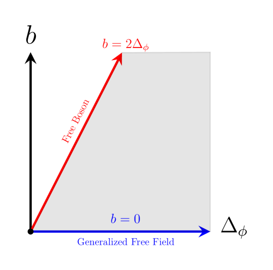
Figure 3: The two-parameter space for the solution $f_{\Delta_{\phi},b}(z,\bar{z})$ to the $2d$ crossing equation. In the shaded region between $0\leq b\leq 2\Delta_{\phi}$ we find numerical evidence that the four-point function $f_{\Delta_{\phi},b}(z,\bar{z})$ has a non-negative expansion on the $SL(2,\mathbb{C})$ blocks. At the two boundaries $b=0$ and $b=2\Delta_{\phi}$, $f_{\Delta_{\phi},b}(z,\bar{z})$ reduces to the four-point functions in the $2d$ generalized free field theory and that in the free boson theory, respectively.

The intermediate spectrum contains the identity operator only if $b=0$ or $b=2\Delta_{\phi}$, which are the lower and upper bounds of $b$ (A.15). In fact, at these values of $b$ the four-point function $f_{\Delta_{\phi},b}(z,\bar{z})$ reduces to known examples:

• $b=0$. In this case $f_{\Delta_{\phi},b=0}(z,\bar{z})$ reduces to the four-point function in the $2d$ generalized free field theory:

  $$f_{\Delta_{\phi},b=0}(z,\bar{z})=1+(z\bar{z})^{\Delta_{\phi}}+\left({z\bar{z}\over(1-z)(1-\bar{z})}\right)^{\Delta_{\phi}}\,.$$ (A.16)

• $b=2\Delta_{\phi}$. In this case $f_{\Delta_{\phi},b=2\Delta_{\phi}}$ reduces to the four-point function of scalar primaries $\cos(\sqrt{\Delta_{\phi}}X)$ in the $2d$ free boson theory:

  $$f_{\Delta_{\phi},b=2\Delta_{\phi}}(z,\bar{z})={1\over 2((1-z)(1-\bar{z}))^{\Delta_{\phi}}}\Big{[}\,(z\bar{z})^{2\Delta_{\phi}}+1+((1-z)(1-\bar{z}))^{2\Delta_{\phi}}\,\Big{]}\,.$$ (A.17)

  Here we have normalized the four-point function by a factor of $1/2$ so that the identity channel comes with unit OPE coefficient. The radius of the free boson does not affect the four-point function as long as the operator $\cos(\sqrt{\Delta_{\phi}}X)$ exists in the spectrum of primaries.

To conclude, $f_{\Delta_{\phi},b}$ provides an interpolation between the four-point function in the $2d$ generalized free field theory and that in the free boson theory (see Figure 3). Even though $f_{\Delta_{\phi},b}$ has no identity channel away from the two limiting cases, we find numerical evidence that it admits a non-negative $SL(2,\mathbb{C})$ block decomposition.

References

• [1] J. de Boer and S. N. Solodukhin, “A Holographic reduction of Minkowski space-time,” Nucl. Phys. B665 (2003) 545–593, hep-th/0303006.
• [2] C. Cheung, A. de la Fuente, and R. Sundrum, “4D scattering amplitudes and asymptotic symmetries from 2D CFT,” JHEP 01 (2017) 112, 1609.00732.
• [3] S. Pasterski, S.-H. Shao, and A. Strominger, “Flat Space Amplitudes and Conformal Symmetry of the Celestial Sphere,” Phys. Rev. D96 (2017), no. 6, 065026, 1701.00049.
• [4] S. Pasterski and S.-H. Shao, “A Conformal Basis for Flat Space Amplitudes,” Phys. Rev. D96 (2017), no. 6, 065022, 1705.01027.
• [5] T. Banks, “A Critique of pure string theory: Heterodox opinions of diverse dimensions,” hep-th/0306074.
• [6] G. Barnich and C. Troessaert, “Symmetries of asymptotically flat 4 dimensional spacetimes at null infinity revisited,” Phys. Rev. Lett. 105 (2010) 111103, 0909.2617.
• [7] G. Barnich and C. Troessaert, “Aspects of the BMS/CFT correspondence,” JHEP 05 (2010) 062, 1001.1541.
• [8] G. Barnich and C. Troessaert, “Supertranslations call for superrotations,” PoS (2010) 010, 1102.4632. [Ann. U. Craiova Phys.21,S11(2011)].
• [9] A. Strominger, “Asymptotic Symmetries of Yang-Mills Theory,” JHEP 07 (2014) 151, 1308.0589.
• [10] D. Kapec, V. Lysov, S. Pasterski, and A. Strominger, “Semiclassical Virasoro symmetry of the quantum gravity $\mathcal{S}$-matrix,” JHEP 08 (2014) 058, 1406.3312.
• [11] T. He, P. Mitra, and A. Strominger, “2D Kac-Moody Symmetry of 4D Yang-Mills Theory,” JHEP 10 (2016) 137, 1503.02663.
• [12] A. E. Lipstein, “Soft Theorems from Conformal Field Theory,” JHEP 06 (2015) 166, 1504.01364.
• [13] C. Cardona, “Asymptotic Symmetries of Yang-Mills with Theta Term and Monopoles,” 1504.05542.
• [14] D. Kapec, P. Mitra, A.-M. Raclariu, and A. Strominger, “A 2D Stress Tensor for 4D Gravity,” 1609.00282.
• [15] T. He, D. Kapec, A.-M. Raclariu, and A. Strominger, “Loop-Corrected Virasoro Symmetry of 4D Quantum Gravity,” 1701.00496.
• [16] A. Strominger, “Lectures on the Infrared Structure of Gravity and Gauge Theory,” 1703.05448.
• [17] A. Nande, M. Pate, and A. Strominger, “Soft Factorization in QED from 2D Kac-Moody Symmetry,” 1705.00608.
• [18] D. Kapec and P. Mitra, “A $d$-Dimensional Stress Tensor for Minkd+2 Gravity,” 1711.04371.
• [19] M. S. Costa, V. Goncalves, and J. Penedones, “Conformal Regge theory,” JHEP 12 (2012) 091, 1209.4355.
• [20] A. Gadde, “In search of conformal theories,” 1702.07362.
• [21] M. Hogervorst and B. C. van Rees, “Crossing Symmetry in Alpha Space,” 1702.08471.
• [22] S. Caron-Huot, “Analyticity in Spin in Conformal Theories,” JHEP 09 (2017) 078, 1703.00278.
• [23] D. Simmons-Duffin, D. Stanford, and E. Witten, “A spacetime derivation of the Lorentzian OPE inversion formula,” 1711.03816.
• [24] S. Ferrara, A. F. Grillo, G. Parisi, and R. Gatto, “The shadow operator formalism for conformal algebra. vacuum expectation values and operator products,” Lett. Nuovo Cim. 4S2 (1972) 115–120. [Lett. Nuovo Cim.4,115(1972)].
• [25] F. A. Dolan and H. Osborn, “Conformal four point functions and the operator product expansion,” Nucl. Phys. B599 (2001) 459–496, hep-th/0011040.
• [26] F. A. Dolan and H. Osborn, “Conformal Partial Waves: Further Mathematical Results,” 1108.6194.
• [27] D. Simmons-Duffin, “Projectors, Shadows, and Conformal Blocks,” JHEP 04 (2014) 146, 1204.3894.
• [28] J. Penedones, “Writing CFT correlation functions as AdS scattering amplitudes,” JHEP 03 (2011) 025, 1011.1485.
• [29] M. S. Costa, V. Gon alves, and J. Penedones, “Spinning AdS Propagators,” JHEP 09 (2014) 064, 1404.5625.
• [30] S. Pasterski, S.-H. Shao, and A. Strominger, “Gluon Amplitudes as 2d Conformal Correlators,” Phys. Rev. D96 (2017) 085006, 1706.03917.
• [31] R. Britto, F. Cachazo, and B. Feng, “New recursion relations for tree amplitudes of gluons,” Nucl. Phys. B715 (2005) 499–522, hep-th/0412308.
• [32] R. Britto, F. Cachazo, B. Feng, and E. Witten, “Direct proof of tree-level recursion relation in Yang-Mills theory,” Phys. Rev. Lett. 94 (2005) 181602, hep-th/0501052.
• [33] S. Pasterski, S.-H. Shao, and A. Strominger , unpublished notes.
• [34] C. Cardona and Y.-t. Huang, “S-matrix singularities and CFT correlation functions,” JHEP 08 (2017) 133, 1702.03283.
• [35] D. Nandan, A. Volovich, C. Wen, and M. Zlotnikov, work in progress.
• [36] M. Gary, S. B. Giddings, and J. Penedones, “Local bulk S-matrix elements and CFT singularities,” Phys. Rev. D80 (2009) 085005, 0903.4437.
• [37] I. Heemskerk, J. Penedones, J. Polchinski, and J. Sully, “Holography from Conformal Field Theory,” JHEP 10 (2009) 079, 0907.0151.
• [38] T. Okuda and J. Penedones, “String scattering in flat space and a scaling limit of Yang-Mills correlators,” Phys. Rev. D83 (2011) 086001, 1002.2641.
• [39] J. Maldacena, D. Simmons-Duffin, and A. Zhiboedov, “Looking for a bulk point,” JHEP 01 (2017) 013, 1509.03612.
• [40] L. Susskind, “Holography in the flat space limit,” hep-th/9901079. [AIP Conf. Proc.493,98(1999)].
• [41] J. Polchinski, “S matrices from AdS space-time,” hep-th/9901076.
• [42] S. B. Giddings, “Flat space scattering and bulk locality in the AdS / CFT correspondence,” Phys. Rev. D61 (2000) 106008, hep-th/9907129.
• [43] A. L. Fitzpatrick, J. Kaplan, J. Penedones, S. Raju, and B. C. van Rees, “A Natural Language for AdS/CFT Correlators,” JHEP 11 (2011) 095, 1107.1499.
• [44] A. L. Fitzpatrick and J. Kaplan, “Scattering States in AdS/CFT,” 1104.2597.
• [45] A. L. Fitzpatrick and J. Kaplan, “Analyticity and the Holographic S-Matrix,” JHEP 10 (2012) 127, 1111.6972.
• [46] A. L. Fitzpatrick and J. Kaplan, “Unitarity and the Holographic S-Matrix,” JHEP 10 (2012) 032, 1112.4845.
• [47] P. A. M. Dirac, “Wave equations in conformal space,” Annals Math. 37 (1936) 429–442.
• [48] G. Mack and A. Salam, “Finite component field representations of the conformal group,” Annals Phys. 53 (1969) 174–202.
• [49] L. Cornalba, M. S. Costa, and J. Penedones, “Deep Inelastic Scattering in Conformal QCD,” JHEP 03 (2010) 133, 0911.0043.
• [50] S. Weinberg, “Six-dimensional Methods for Four-dimensional Conformal Field Theories,” Phys. Rev. D82 (2010) 045031, 1006.3480.
• [51] M. S. Costa, J. Penedones, D. Poland, and S. Rychkov, “Spinning Conformal Correlators,” JHEP 11 (2011) 071, 1107.3554.
• [52] M. S. Costa, J. Penedones, D. Poland, and S. Rychkov, “Spinning Conformal Blocks,” JHEP 11 (2011) 154, 1109.6321.
• [53] M. Campiglia, “Null to time-like infinity Green’s functions for asymptotic symmetries in Minkowski spacetime,” JHEP 11 (2015) 160, 1509.01408.
• [54] M. Campiglia, L. Coito, and S. Mizera, “Can scalars have asymptotic symmetries?,” 1703.07885.
• [55] E. Witten, “Anti-de Sitter space and holography,” Adv. Theor. Math. Phys. 2 (1998) 253–291, hep-th/9802150.
• [56] J. Maldacena and D. Stanford, “Remarks on the Sachdev-Ye-Kitaev model,” Phys. Rev. D94 (2016), no. 10, 106002, 1604.07818.
• [57] E. Hijano, P. Kraus, E. Perlmutter, and R. Snively, “Witten Diagrams Revisited: The AdS Geometry of Conformal Blocks,” JHEP 01 (2016) 146, 1508.00501.
• [58] M. F. Paulos, J. Penedones, J. Toledo, B. C. van Rees, and P. Vieira, “The S-matrix Bootstrap I: QFT in AdS,” 1607.06109.
• [59] T. Hartman, S. Jain, and S. Kundu, “Causality Constraints in Conformal Field Theory,” JHEP 05 (2016) 099, 1509.00014.
• [60] S. Ferrara, R. Gatto, and A. F. Grillo, “Properties of Partial Wave Amplitudes in Conformal Invariant Field Theories,” Nuovo Cim. A26 (1975) 226.
• [61] F. A. Dolan and H. Osborn, “Conformal partial waves and the operator product expansion,” Nucl. Phys. B678 (2004) 491–507, hep-th/0309180.