Galaxy And Mass Assembly: Automatic Morphological Classification of Galaxies Using Statistical Learning

Abstract

We apply four statistical learning methods to a sample of $7941$ galaxies ($z<0.06$) from the Galaxy and Mass Assembly (GAMA) survey to test the feasibility of using automated algorithms to classify galaxies. Using $10$ features measured for each galaxy (sizes, colours, shape parameters & stellar mass) we apply the techniques of Support Vector Machines (SVM), Classification Trees (CT), Classification Trees with Random Forest (CTRF) and Neural Networks (NN), returning True Prediction Ratios (TPRs) of $75.8\%$, $69.0\%$, $76.2\%$ and $76.0\%$ respectively. Those occasions whereby all four algorithms agree with each other yet disagree with the visual classification (‘unanimous disagreement’) serves as a potential indicator of human error in classification, occurring in $\sim 9\%$ of ellipticals, $\sim 9\%$ of Little Blue Spheroids, $\sim 14\%$ of early-type spirals, $\sim 21\%$ of intermediate-type spirals and $\sim 4\%$ of late-type spirals & irregulars. We observe that the choice of parameters rather than that of algorithms is more crucial in determining classification accuracy. Due to its simplicity in formulation and implementation, we recommend the CTRF algorithm for classifying future galaxy datasets. Adopting the CTRF algorithm, the TPRs of the 5 galaxy types are : E, $70.1\%$; LBS, $75.6\%$; S0-Sa, $63.6\%$; Sab-Scd, $56.4\%$ and Sd-Irr, $88.9\%$. Further, we train a binary classifier using this CTRF algorithm that divides galaxies into spheroid-dominated (E, LBS & S0-Sa) and disk-dominated (Sab-Scd & Sd-Irr), achieving an overall accuracy of $89.8\%$. This translates into an accuracy of $84.9\%$ for spheroid-dominated systems and $92.5\%$ for disk-dominated systems.

Keywords: galaxies, automated morphological classification, statistical learning, machine learning algorithms.

1 Introduction

Galaxies are observed to have a wide variety of forms, from bright massive ellipticals to extended late-type spirals and faint compact dwarfs. One of the first attempts in categorising galaxies by their visual appearance was proposed by Wolf (1908). These so-called ‘galactic nebulae’ were arranged according to their shape, size and distinguishing features. No continuity or transition between these groupings was suggested. As imaging technology improved over the course of the next decade and available datasets grew, new systems for galaxy classification were proposed by many authors (e.g.: Jeans, 1919; Reynolds, 1920). This culminated in the development of the Hubble (1936) sequence or tuning fork. The Hubble tuning fork divides galaxies into early type: typically red and smooth ellipticals; late type: typically blue extended disk-like spirals, both barred and unbarred, and; a bridging population of lenticulars: systems with both a smooth bulge component and an extended yet smooth disk component. Subsequent extensions to the Hubble tuning fork have addressed a number of shortcomings in the initial classification methodology. These include the inclusion of bulge-less spirals (Shapley & Paraskevopoulos, 1940), transition lenticulars (Holmberg, 1958), rings (de Vaucouleurs, 1959), barred lenticulars (Sandage, 1961; Sandage et al., 1975) and dwarfs/irregulars (Sandage & Binggeli, 1984). The success of this relatively simple and extensible schema for morphological classification of galaxies has ensured that the Hubble tuning fork remains relevant almost a century later.

Hubble type classifications have been used to explore a number of astrophysical phenomena. It was initially noted by Hubble & Humason (1931) that elliptical and lenticular galaxies preferentially favour galaxy cluster environments, indicating a potential environmental dependence on galaxy morphology. Oemler (1974) built upon this work some decades later, showing that the early type galaxy fraction increases in dense regions. Dressler (1980) conclusively showed how the fractions of elliptical, lenticular and spiral+irregular galaxies varied as a function of projected galaxy density: the morphology-density relation. He found that dense regions such as galaxy groups and clusters preferentially harbour elliptical galaxies, whilst less dense ‘field’ regions host lenticular, spiral and irregular galaxies (See also Smith et al. 2005). This apparent relation between morphology and environment has been further explored in recent years to encompass, amongst others, galaxy mass (van der Wel, 2008), star formation (Welikala et al., 2008, 2009), colour (Bamford et al., 2009), the galaxy luminosity function (Kelvin et al., 2014a, see also Baldry et al., 2006), the galaxy stellar mass function (Kelvin et al., 2014b) and galaxy structure (Hiemer et al., 2014).

Precisely how galaxies form and evolve into their various morphological configurations, and the dependence of this on environment, has been the subject of much investigation. Spitzer & Baade (1951) first suggested that merging events between galaxies, more common in dense cluster environments, may be responsible for their transition from a spiral to a lenticular morphology. Toomre (1977) went further, suggesting that elliptical galaxies may also be formed via this merging mechanism (see also White & Rees, 1978). In addition to merging, a number of supplementary processes which act to modify the morphology of a galaxy have been proposed, including ram pressure stripping of spiral gas as a galaxy travels through a hot dense intracluster medium (Gunn & Gott, 1972), the rapid decline of star-formation due to a loss of its hot gas resevoir (strangulation: Larson et al., 1980; Kauffmann et al., 1993; Balogh et al., 2000; Diaferio et al., 2001), heating of the galaxy caused by rapid encounters with other nearby systems (harassment: Moore et al., 1996) and tidal interations (Moss & Whittle, 2000; Gnedin, 2003b, a; Park et al., 2008). Obtaining an accurate estimate of galaxy morphology is therefore essential in order to facilitate exploration of the formation and evolution of galaxies.

Contemporary catalogues of galaxy morphology vary in size and classification methodology. Kelvin et al. (2014a) (also Moffett et al., 2016) morphologically classify a local volume-limited sample of galaxies taken from the Galaxy And Mass Assembly (GAMA, Driver et al., 2009) survey. Classification is performed via majority observer consensus based on visual inspection of a composite three-colour optical-NIR image. Three independent expert classifiers are asked a series of questions for each galaxy: is the galaxy spheroid or disk dominated, is the galaxy a single or multi-component system, and is the galaxy barred or unbarred. This allows for the galaxy sample to be principally divided into elliptical (E), early-type spiral (S0-Sa), intermediate-type spiral (Sab-Scd) and late-type spiral/irregular (Sd-Irr). Additional barred classes for early-type and intermediate-type spirals (SB0-SBa and SBab-SBcd, respectively) are also present. A small subset of ‘little blue spheroid’ (LBS) galaxies, blue compact systems ($\sim 7.4$%), did not fit into this classification hierarchy and were excluded at the top level. This methodology produces accurate classifications yet remains a time consuming exercise, a problem which will only become more acute as future datasets increase in size.

A novel alternative is to enlist the support of the wider astronomy community. The Galaxy Zoo project (Lintott et al., 2008) allows for volunteer ‘citizen scientists’ to visually classify galaxies via a web interface. The simple and effective design of the website allows for a large number of classifiers to visit each galaxy (typically of the order $\sim 60$), enabling rapid classification of large datasets. However, future facilities such as the Euclid space telescope and Large Synoptic Survey Telescope (LSST) will probe much larger volumes, providing datasets for several billion galaxies. For these future facilities, morphological classification via visual inspection becomes increasingly prohibitive.

The concept of using automated techniques to quantify galaxy morphologies stem from this ‘big data overload’ scenario. Moore et al. (2006) demonstrated the use of an automated Mathematical Morphology algorithm to achieve classification into ellipticals and late-type spirals using the images from Smail et al. (1997). Their approach was unique in that it had fewer free parameters and that it didn’t require a classifier to be trained with a machine learning algorithm. Another widely used approach to classify galaxies is by the application of statistical machine learning algorithms. Those that have been used previously used include artificial neural networks, Support Vector Machines (SVM), decision trees and random forests. They are applied to either galaxy images or to parameters extracted from imaging and spectroscopic data. As part of the Kaggle challenge conducted by the Galaxy Zoo team, Dieleman et al. (2015) presented a convolutional neural network approach (ConvNets) to classify galaxy images. Their algorithm was designed to operate with a training set of $55,420$ galaxy images, real time evaluation set of $6158$ images and a test set of $79,975$ images. Huertas-Company et al. (2015) applied this algorithm to $58,000$ (47,700 training, 5300 validation and 5000 testing) high redshift galaxy images(median redshift $z\sim 1.25$) from 5 Cosmic Assembly Near-infrared Deep Extragalactic Legacy Survey (CANDELS) fields with a result of $<1\%$ misclassifications.

Abraham et al. (1996) introduced a new method of discerning between early, late and irregular type galaxies, the C-A plane, where C stands for the central concentration and A for the rotational asymmetry of the galaxy. This was based on Okamura et al. (1984) and Doi et al. (1993), both of whom proposed a strong correlation between the mean concentration index and galaxy morphology. The logged values of these two parameters are plotted in a 2-D plane and the separation between the different galaxy populations are obtained by applying linear boundaries. Conselice (2003) expanded upon this method by adding a third dimension, smoothness or clumpiness of the galaxy (represented by S). He was also among the first groups to consider additional morphological types such as dwarf ellipticals, dwarf irregulars and mergers. For more than three dimensions , this method becomes difficult. Also, it presents some problems when it comes to ground based, high redshift data. Graham et al. (2001) revealed that the concentration parameter, C was unstable in nature due to its high sensitivity to the image exposure depth. Conselice (2003) explains that while it is possible to obtain average values for CAS parameters for data from space-based telescopes (deep Hubble Space Telescope data being the example in the paper) up to a redshift $z\sim 3$, the same values for single galaxies will have such high uncertainties that their usage will be quite limited until such a time when deeper and high resolution imaging can be taken.

Huertas-Company et al. (2007) offered a generalisation of the CAS method using SVM. Other examples from literature where a statistical learning technique was used to classify galaxies include Banerji et al. (2010) (artificial neural networks), Owens et al. (1996) (oblique decision trees) and Gauci et al. (2010) (three decision tree algorithms including a random forest approach). All these methods use measured parameters as inputs to the classifying algorithms.

The goal of this paper is to explore the viability in using statistical learning methods to produce robust automated Hubble-type morphology catalogues for datasets with a greater variety in galaxy types. We have attempted to formulate a general method that will be applicable to small data sets and surveys that do not have access to such a wide variety of parameters as we do. Section 2 details the GAMA (Driver et al., 2009) dataset used in this study. Section 3 describes the various statistical learning algorithms under consideration and the application of these algorithms to the dataset. Results are shown in Section 4 and the conclusions and future prospects are presented in Section 5. Unless otherwise stated, a standard cosmology of $\left(H_{0},\Omega_{m},\Omega_{\Lambda}\right)=\left(70\mathrm{\,km\,s^{-1}\,Mpc^{-1}},0.3,0.7\right)$ is assumed throughout this paper.

2 Data

In this section we briefly describe the GAMA survey from which our data sample is taken, the parameters that we have chosen and the justifications for choosing these specific parameters.

2.1 Galaxy And Mass Assembly (GAMA)

GAMA is a project designed to study the low redshift galaxy population, combining data from eight ground-based and four space-based facilities. It involves both spectroscopic and multi-wavelength imaging programmes which are designed to study structures along the scales from 1 kiloparsec (kpc) to 1 megaparsec (Mpc) in the nearby Universe ($z\mathrel{\hbox{\hbox to0.0pt{\hbox{\lower 4.0pt\hbox{$\sim$}}\hss}\hbox{$<$}}}0.25$). The main goal of the GAMA survey is to test and verify the hierarchical structure formation scenario that emerges from the $\Lambda$CDM cosmological model by measuring the structure growth rate, halo mass function and star forming efficiency of galaxies in groups.

The GAMA spectroscopic survey was carried out on the AAOmega multi-object spectrograph on the Anglo-Australian Telesecope (AAT). It includes $\sim 300,000$ galaxies with magnitudes down to r $\sim 19.8$ mag (r being the Galactic extinction corrected Petrosian magnitude in the r-band from SDSS DR6; Adelman-McCarthy et al. 2008) spanning an area of $\sim 286$ deg². The GAMA imaging programme compiles and reprocesses data from a number of other contemporary imaging surveys (see Driver et al. 2009 for details). The reprocessed optical and near-infrared imaging has a pixel-scale resolution of $0.339$ arcseconds/pixel. The master GAMA input catalogue, InputCatAv07, is primarily based on SDSS DR7 (Abazajian et al., 2009) photometry. The majority of the redshifts have been attained as part of the GAMA spectroscopic campaign on the AAT (Hopkins et al., 2013). Additional redshifts are obtained from a number of surveys including the SDSS (Smee et al., 2013), 2dFGRS (Colless et al., 2001), MGC (Driver et al., 2005) and others. Full details may be found in Driver et al. (2009) and Baldry et al. (2014).

Table 1: Hubble type classifications in the GAMA Catalogue and their distribution in our data set. The complete data set consists of 7941 objects from which we remove 374 objects that are visually classified as a ‘star’ or ‘artefact’ (GAMA Hubble types 50 and 60) and 39 objects that do not have valid values for the parameters we have chosen. Of the remaining 7528 objects, we combine the unbarred (11) and barred (12) early type spirals as well as the unbarred (13) and barred (14) intermediate-type spirals to form two new composite data types 1112 and 1314 (henceforth combinedly referred to as S0-Sa and Sab-Scd respectively).

GAMA Hubble type code	Galaxy type	Abbreviation	Number of objects (% in final 7528 sample)	Of which in training set	Of which in test set
1	Elliptical	E	856 ($11.4\%\pm 3.3$)	682 (11.3%)	174 (11.6%)
2	Little Blue Spheroid	LBS	869 ($11.5\%\pm 2.0$)	689 (11.4%)	180 (12.0%)
11	Early-type spirals	S0-Sa    }312pt	833 ($11.1\%\pm 0.7$)	657 (10.9%)	176 (11.7%)
12	Early-type spirals (barred)	SB0-SBa
13	Intermediate-type spirals	Sab-Scd    }312pt	1432 ($19.0\%\pm 6.2$)	1152 (19.1%)	280 (18.6%)
14	Intermediate-type spirals (barred)	SBab-SBcd
15	Late-type spirals & Irregulars	Sd-Irr	3538 ($47.0\%\pm 5.9$)	2842 (47.2%)	696 (46.2%)
50	Artefact	Artefact    }312pt	374	-	-
60	Star	Star
-	Incomplete features	-	39	-	-

Note: Additional Hubble types of Not Elliptical ($10$) and Uncertain ($70$) Morphologies are available in the GAMA VisualMorphology DMU, though these were derived for a different sample via a different method and as such are not used in this study (see Driver et al. 2012 for further details).

Table 2: Parameters chosen from the GAMA catalogues and the derived parameters used for training and testing our algorithms. The parameters in the top panel are those given to the machine learning algorithms as input. Those in the bottom panel are used to derive those in the top panel (with the exception of visual Hubble type), but were not used directly.

Parameter Name	Catalogue column name	Notes	Units	Table	Reference
Stellar mass	logmstar	logged in catalogue	$\log_{10}(M_{\odot})$	StellarMassesv18	Taylor et al. (2011)
Mass-to-light ratio	logmoverl_i	logged in catalogue	$\log_{10}(M_{\odot}/L_{\odot,i})$	StellarMassesv18	Taylor et al. (2011)
$g-i$ colour	gminusi	not logged	mag	StellarMassesv18	Taylor et al. (2011)
$u-r$ colour	uminusr	not logged	mag	StellarMassesv18	Taylor et al. (2011)
Absolute magnitude	absmag_r	not logged	mag	StellarMassesv18	Taylor et al. (2011)
Ellipticity	GALELLIP_r	not logged	no unit	SersicCatSDSSv09	Kelvin et al. (2012)
Sérsic index	GALINDEX_r	logged	no unit	SersicCatSDSSv09	Kelvin et al. (2012)
Half-light radius in kpc	-	logged	$\log_{10}(kpc)$	-	-
Kron radius in kpc (semi-major axis)	-	logged	$\log_{10}(kpc)$	-	-
Kron radius in kpc (semi-minor axis)	-	logged	$\log_{10}(kpc)$	-	-
Half-light radius	GALRE_r	-	arcsec	SersicCatSDSSv09	Kelvin et al. (2012)
Kron radius	KRON_RADIUS	-	units of A_IMAGE or B_IMAGE	ApMatchedCatv06	Hill et al. (2011)
Angular size (semi-major axis)	A_IMAGE	used to calculate Kron radius in kpc	pixels	ApMatchedCatv06	Hill et al. (2011)
Angular size (semi-minor axis)	B_IMAGE	used to calculate Kron radius in kpc	pixels	ApMatchedCatv06	Hill et al. (2011)
Redshift	Z_TONRY	used to calculate Kron and half-light radii in kpc	no unit	DistancesFramesv14	Baldry et al. (2012)
Hubble type	HUBBLE_TYPE_CODE	barred and unbarred counterparts merged for training the algorithms	no unit	VisualMorphologyv02	Kelvin et al. (2014a) Moffett et al. (2016)

2.2 Galaxy Sample

The galaxy sample used in this paper is from Data Release 2 of the GAMA survey (Liske et al., 2015) which gives spectra, redshifts and supplementary information regarding $72,225$ objects from GAMA Data Release 1 (Driver et al., 2011). Our primary sample consists of $7941$ galaxies which have been visually classified into $11$ Hubble types (Kelvin et al. 2014a, Moffett et al. 2016 ; see Table 1; refer to the VisualMorphologyv02 catalogue in the VisualMorphology DMU for further details), spanning a redshift range of $0.002\leq z\leq 0.06$.

From our intial sample of $7941$ galaxies, we have excluded those objects that are classified as a ‘star’ or ‘artefact’ (GAMA Hubble type codes $50$ and $60$; 374 in number) in the VisualMorphology02 catalogue. We have also excluded an additional $39$ objects for which the values were missing for one or more of our chosen parameters. Therefore the final sample that we apply our statistical learning methods to consists of $7528$ objects. Of these, the number of objects of each morphological type are : ellipticals - 856 ($11.4\%\pm 3.3$), LBS - 869 ($11.5\%\pm 2.0$), early-type spirals - 833 ($11.1\%\pm 0.7$), intermediate-type spirals - 1432 ($19.0\%\pm 6.0$) and late-type spirals & irregulars - 3538 ($47.0\%\pm 5.9$). We computed uncertainties in the sample based on standard deviations of the classifications by the three human classifiers.

2.3 Chosen Parameters

The choice of input parameters is crucial for the effectiveness of statistical learning algorithms. We want to recreate the classification process that the human eye would perform upon seeing an image, using parameters extracted from such an image. Ideally we would choose parameters that clearly demarcate the different classes of galaxies. Table 2 lists the parameters that we have chosen from the GAMA database for each galaxy, the tables they have been taken from and the relevant references.

It is decidedly non-trivial to differentiate between galaxies using only parameters that give similar information, for example, galaxy colour. In Lange et al. (2015), the separation between early and late type galaxies in the GAMA catalogue are defined as $u-r=1.5$ mag and $g-i=0.65$ mag. Values greater than these would represent the redder (early-type) galaxies while values less than these would represent bluer (late-type) galaxies. Using only colour to ascribe morphology of a galaxy gives a good general picture of the apparent bimodality of the local galaxy population, but neglects the fact that colour traces star formation while morphology reflects the dynamic evolution of the galaxy. While they are related, they are not the same. The colour information alone may bias against certain morphological types such as blue ellipticals and red spirals (see Figure 20 of Kelvin et al. 2012). The addition of extra features such as Sérsic index undoubtedly helps provide a more accurate separation of early and late type galaxies (Driver et al. 2006; Cameron et al. 2009).

Our objective has been to choose a broad range of parameters that will allow us to successfully morphologically classify galaxies with minimal failures. We have been careful to select astrophysically meaningful parameters that denote different aspects of the physicality of a galaxy. As listed in Table 2, we have parameters that are known to directly trace galaxy morphology (Sérsic index, stellar mass, colour), parameters that trace galaxy morphology indirectly (mass-to-light ratio) and parameters that are based on galaxy structure (Kron radius, ellipticity, half-light radius and absolute magnitude). We have attempted to remove the effects of redshift on all the chosen parameters. We also note that in this work, we haven’t accounted for the errors in the chosen set of parameters.

The total stellar mass, mass-to-light ratio, absolute magnitude, $g-i$ and $u-r$ colours are taken from the table StellarMassesv18 in the GAMA Data Management Unit (DMU) Stellar Masses (Taylor et al., 2011). Total stellar masses have been derived using Stellar Population Synthesis (SPS) modelling using Bruzual and Charlot models (Bruzual & Charlot, 2003) assuming a Chabrier initial mass function (Chabrier, 2005). SDSS and VISTA-VIKING photometry have been used for this calculation (roughly equivalent to restframe $u-Y$). The mass-to-light ratio has been calculated using the SDSS restframe i-band. The $g-i$ and $u-r$ colours are restframe colours using AB photometry that has been k-corrected to redshift $z=0$ calculated from the Spectral Energy Distribution fit. Together, these colours provide a wide wavelength baseline. Absolute magnitude has been calculated using the restframe r-band from the best SPS SED fit.

Ellipticity, Sérsic index and half-light radius have been taken from the table SersicCatSDSSv09 in the DMU Sérsic Photometry (Kelvin et al., 2012). These are based on 2-D single Sérsic function fits to SDSS r-band images.

We obtained Kron radii in arcseconds by multiplying the Kron radius with the angular sizes in semi-major and minor axes and the angular resolution of the main GAMA imaging dataset (0.339"/pixel). These values were converted into kpcs using flow-corrected spectroscopic redshifts from the catalogue DistancesFramesv14 (Baldry et al., 2012).

We use morphology for training purposes and to test the robustness of our algorithms. We also note that our parent sample (Kelvin et al. 2014a; Moffett et al. 2016) is magnitude limited ($M_{r}<-17.4$ mag) and we do not expect it to be overly sensitive to dwarf galaxy populations. The complete list of parameters that we have used for training and testing are given in Table 2.

2.4 Principal Component Analysis

We perform Principal Component Analysis (PCA, Pearson 1901) on the parameters that we have chosen from the GAMA catalogues (see Section 2.3, Table 2). PCA is one of the methods by which parameters are generally chosen for functions such as classification. In our case, we had already defined the criterion for choice of parameters as their distance independence or the possibility of removal of their distance dependence. Therefore, our PCA is a secondary method, to see statistically, the impact each parameter has on the classification process. It was done using the MATLAB function pca. Approximately $86\%$ of the variability in our parameters is contained in Components $1-3$ of PCA. For visualisation convenience, we have plotted the first two components in Figure 1.

Of the two plotted components, Component 1 contains $\sim 57\%$ of the variance of the parameters and Component 2 contains $\sim 17\%$. Both stellar mass (logmstar) and absolute magnitude (absmag) have a significant impact on Component 1, but a smaller contribution towards Component 2. The parameters $g-i$ (g-i) and $u-r$ (u-r) colours and mass-to-light ratio (m/l) have very similar contributions to both the components, and are therefore redundant to a great extent.

Of the other parameters that we have chosen, Sérsic index (n), Kron radii ($Kron_{A}$ and $Kron_{B}$) and half-light radius ($R_{e}$) seem to have significant contributions toward both Components 1 & 2, thereby representing sizeable variability in the data set. Ellipticity (ell) seems to be the one with the least variance among our parameters. A detailed analysis of how much each parameter affects the classification process is given in Section 4.

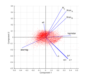
Figure 1: Results of Principal Component Analysis (PCA) performed on the selected parameters to determine their impacts on the classification process. The component labels correspond to the parameters given in Table 2 in the following manner: ell = ellipticity; $R_{e}$ = half-light radius in kpc; $Kron_{A}$ = Kron radius in kpc (major axis); $Kron_{B}$ = Kron radius in kpc (minor axis); logmstar = stellar mass; g-i = $g-i$ colour; u-r = $u-r$ colour; $m/l$ = mass-to-light ratio; n = Sérsic index; absmag = absolute magnitude. Please see Table 2 for more details. The analysis was performed using the MATLAB function pca.

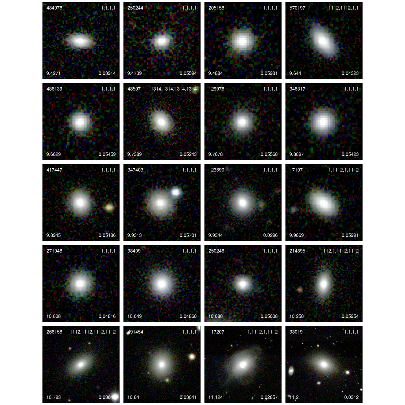
Figure 2: A sample of galaxies classified as elliptical (type 1, E) in the GAMA visual morphology catalogue. Postage stamps are log scaled, span an area of 3 $\times$ Kron radius of each galaxy, and are ordered from top-left to bottom-right by increasing stellar mass. Overlaid on each galaxy image are: (top left) the GAMA CATAID of the galaxy; (top right) the numeric Hubble type codes indicating the predicted classification as determined by the SVM, CT, CTRF and NN classifiers, respectively; (bottom left) the total stellar mass in units of $\log_{10}(M_{\odot})$, and; (bottom right) the flow corrected spectroscopic redshift of the galaxy. The row-wise median physical scales for these galaxies in kiloparsecs are 5.5, 5.4, 7.4, 7.5 and 2.9.

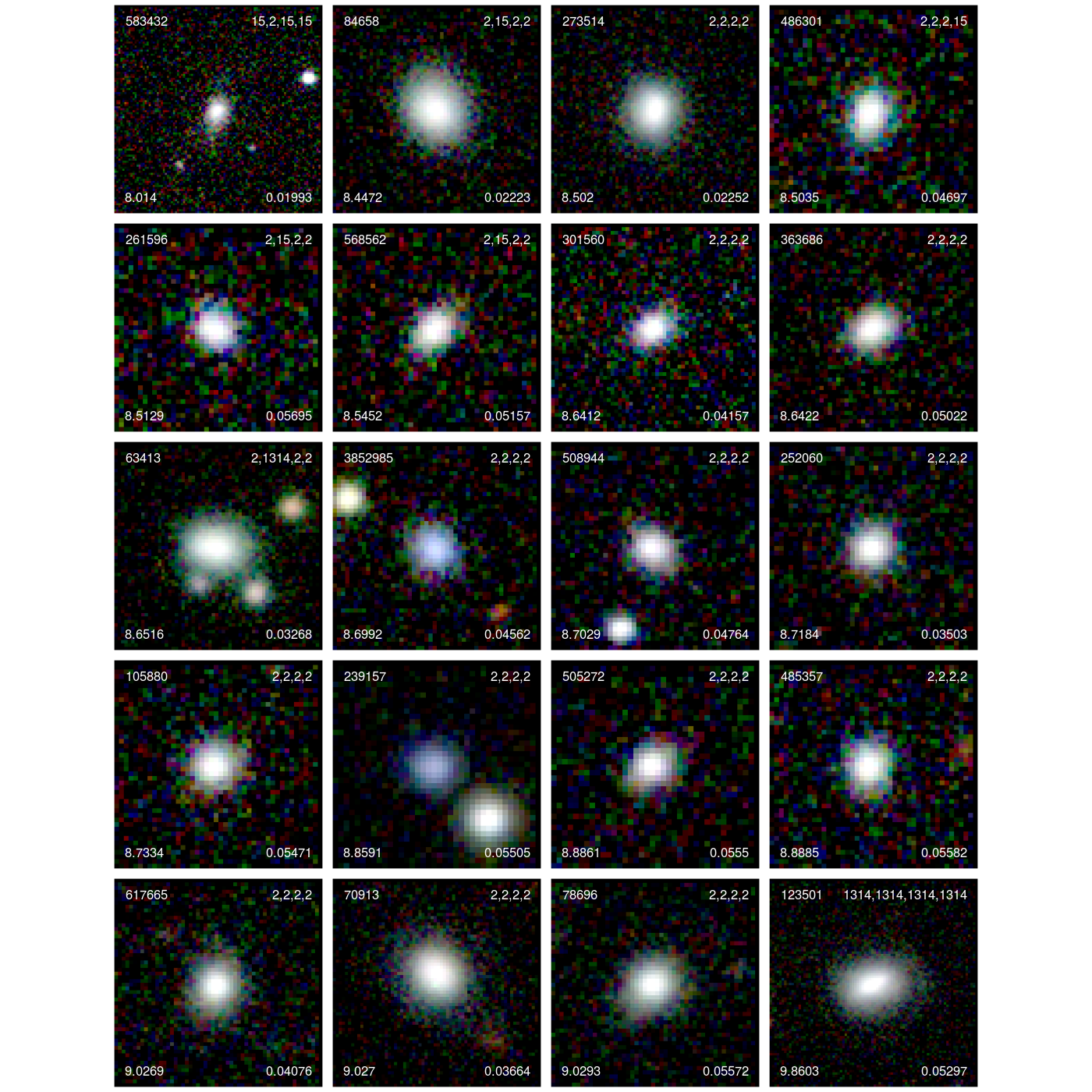
Figure 3: As Figure 2, but for Little Blue Spheroid (type 2, LBS) galaxies. The row-wise median physical scales for these galaxies in kiloparsecs are 4.6, 5.1, 4.0, 5.0 and 19.0.

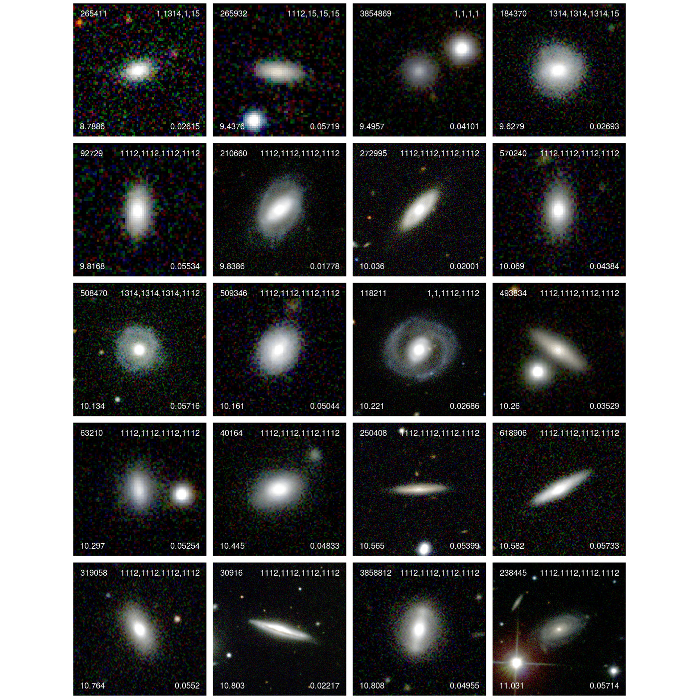
Figure 4: As Figure 2, but for early-type spiral (type 1112, S0-Sa) galaxies. The row-wise median physical scales for these galaxies in kiloparsecs are 15.9, 24.3, 17.4, 13.5 and 11.8.

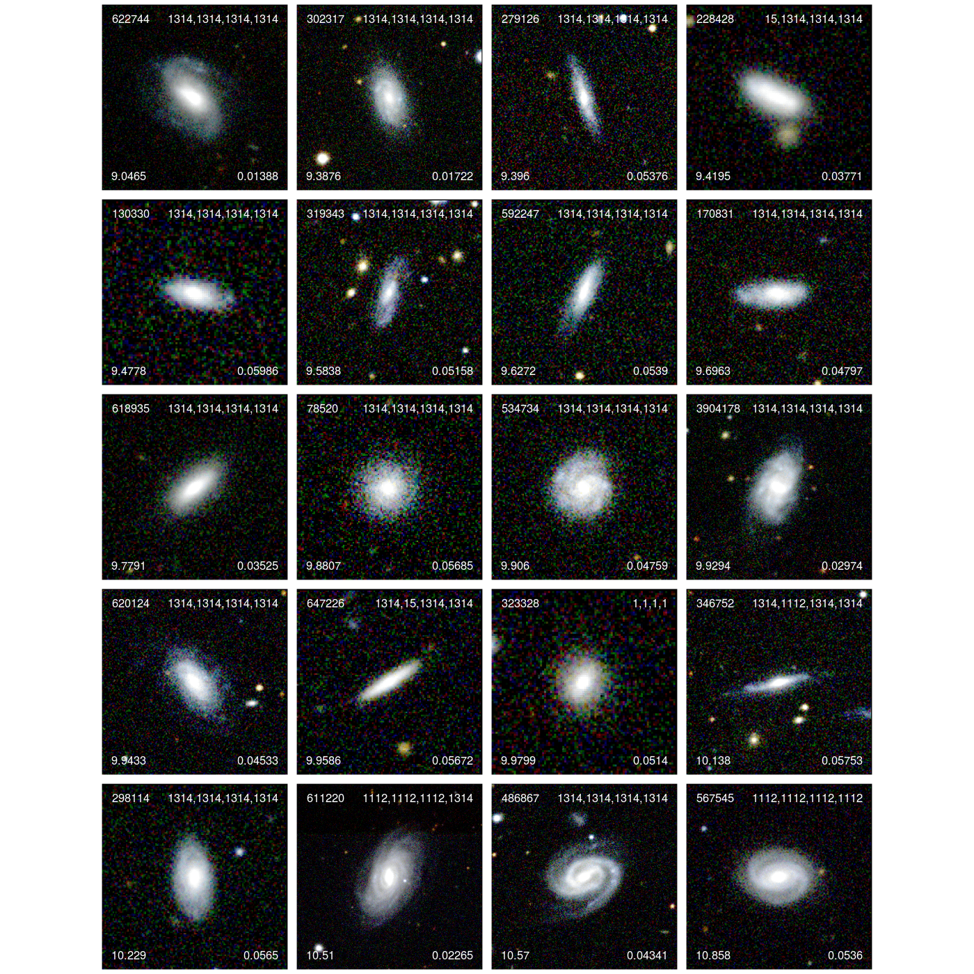
Figure 5: As Figure 2, but for intermediate-type spiral (type 1314, Sab-Scd) galaxies. The row-wise median physical scales for these galaxies in kiloparsecs are 12.5, 21.8, 12.4, 17.5 and 18.1.

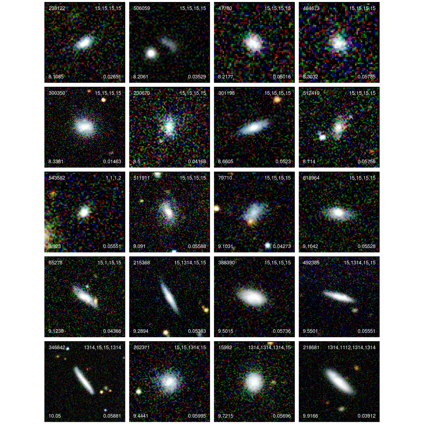
Figure 6: As Figure 2, but for late-type spiral & irregular (type 15, Sd-Irr) galaxies. The row-wise median physical scales for these galaxies in kiloparsecs are 28.9, 9.6, 8.1, 12.4 and 17.0.

2.5 Data preprocessing

Classes $12$ and $14$ are the barred counterparts of classes $11$ and $13$. Their numbers are low in our sample, at $80$ and $195$ respectively. A potential reason for this, as noted in Kelvin et al. (2014a) is that there were noticeable disagreements among the classifiers about the presence of bars in these systems. Another reason could be that, for edge-on systems, it is impossible to verify the presence of bars and therefore they would be classified as unbarred. Due to the relatively low numbers of galaxy systems hosting bars in our sample, we opt to merge the barred classes with their unbarred counterparts. We merge the classes $11$ and $12$ (S0-Sa & SB0-SBa) to form a new class $1112$. Likewise, we merge classes $13$ and $14$ (Sab-Scd & SBab-SBcd) to form a new class $1314$. This simplifies the classification problem, albeit marginally. The machine learning classifier that we formulate concentrates on predicting the GAMA Hubble Types $1$, $2$, $1112$, $1314$ and $15$. Figures 2-6 show examples of each galaxy type from our final sample. They are created using SDSS g, r, and i band imaging by the GAMA Panchromatic Swarp Imager (PSI) tool. Each image spans a diameter equivalent to 3 $\times$ Kron radius of the galaxy in arcseconds, and is log scaled.

To construct and evaluate classifiers using statistical learning methods, the data sample is randomly split into training and test sets. The training set is used for constructing classifiers, containing $80\%$ of the data sample. The test set is used for the evaluation of the classifiers’ prediction abilities, containing the remaining $20\%$ of galaxies. In our case the training and test sets contain $6022$ and $1506$ galaxies respectively. We consistently use the same training and test sets for all considered statistical learning methods described in Section 3. The data are normalised before training, i.e. we centre each parameter at its mean value, and scale it to have unit standard deviation. The distribution of Hubble types for the full data sample, training and test subsets are presented in Table 1.

3 Methods

In this section, we outline the galaxy classification problem in the context of statistical learning. We also describe the methods that we apply to solve this classification problem.

3.1 The classification problem

We consider the parameters of a galaxy to be components of a multidimensional vector $\mathbf{x}=\left(x_{1},x_{2},\dots,x_{p}\right)^{\top}\in{\mathbb{R}}^{p}$, where $\left(\cdot\right)^{\top}$ denotes the transpose of a vector or matrix. Thus, $\mathbf{x}$ is a $p\times 1$ column vector. In our case $p=10$, and we use the parameters described in Table 2.

In the context of statistical learning, the vector space ${\mathbb{R}}^{p}$ is often called feature space, the elements $\mathbf{x}\in{\mathbb{R}}^{p}$ are called feature vectors, and the components $x_{i}$ of the feature vectors are called features. The feature vector $\mathbf{x}$ belongs to one of the $T$ classes. For convenience, we label the classes as $1,2,\dots,T$. In our case $T=5$, and the classes correspond to the considered Hubble Types (HT) as $\Set{1,2,1112,1314,15}\widehat{=}\Set{1,2,3,4,5}$. Let $y\in\Set{1,2,\dots,T}$ denote the class label of $\mathbf{x}$.

Suppose that there is an ideal classifier $f^{*}\colon\mathbf{x}\mapsto y$ that for each feature vector $\mathbf{x}$ assigns its true classification $y$. A statistical learning method aims to construct a classifier $f\colon\mathbf{x}\mapsto y$ that approximates $f^{*}$. For this purpose, statistical learning methods use observational data of the pairs $\left(\mathbf{x}_{i},y_{i}\right)$ that contain feature vectors $\mathbf{x}_{i}$ for which the corresponding class $y_{i}$ is known. A set made up of such pairs $\left(\mathbf{x}_{i},y_{i}\right)$ is called the training set, and we denote it as $\mathcal{Z}=\Set{\left(\mathbf{x}_{i},y_{i}\right),\;i=1,2,\dots,N}$.

Every statistical learning method consists of a family of classifiers $f$ that depends on certain parameters. Using a learning procedure, a particular classifier is chosen from this family based on the classifier’s behaviour on the training data set. The selection is typically done such that the classification is well predicted on the training set, i.e. $f\left(\mathbf{x}_{i}\right)\approx y_{i}$, so as to give low training errors. The quality of the classifier is then evaluated on the test set, where the classification is known. The data of the test set is not used for constructing the classifier. Thus, the performance of the classifier on the test set can be seen as an estimation of its performance on sets with unknown classification.

The methods that we consider here for classifying galaxies are: Support Vector Machines (SVM), Classification Trees (CT), Classification Trees with Random Forest (CTRF) and Neural Networks (NN). We have used the realisation of these methods in MATLAB R2014b. The outputs provided by the algorithms that we have formulated are multi-class labels, denoting which galaxy type the algorithms deem the galaxy to be of. They are described in detail in the following subsections.

3.2 Support Vector Machines (SVM)

The SVM method was originally designed for binary classification (Cristianini & Shawe-Taylor 2000; Hastie et al. 2009, Chapter 12). In this method, for each feature vector $\mathbf{x}$ there is a class label $z\in\Set{-1,1}$. Therefore for each $\mathbf{x}_{i}$ in the training set, the corresponding class is $z_{i}$. The details of the structure and definitions of the SVM classifier that we employ are given in Appendix A.1.

We use the MATLAB function svmtrain for constructing SVM classifiers. For computing the result $f\left(\mathbf{x}\right)$ of the SVM classifier $f$, function svmclassify has been used.

In order to use SVM for multi-class classification, the multi-class classification problem is reduced into a series of binary classification problems. For this purpose, we consider a tree structure approach (Campbell, 2001). We propose a tree formed by the binary classifiers $C_{\mathrm{15}}$, $C_{\mathrm{sp}}$, $C_{\mathrm{E}}$, $C_{\mathrm{a}}$ as depicted in Figure 7. This tree structure is inspired by the distribution of Hubble types in our dataset represented in Table 1. Here, $C_{\mathrm{15}}$ is the binary classifier that classifies a galaxy as HT 15 or not. $C_{\mathrm{sp}}$ then classifies into spirals and not spirals. Further classification is done by $C_{\mathrm{E}}$ into HT 1 (E) or HT 2 (LBS). $C_{\mathrm{a}}$ splits the output of the $C_{\mathrm{sp}}$ binary classifier into HTs 1112 and 1314. All the binary classifiers in this tree structure are constructed with the SVM method. At each binary classifier, the data is split by roughly $50\%$.

Figure 7: The binary classification tree determined for the SVM method. The classifier $C_{\mathrm{15}}$ classifies a galaxy as HT 15 or not. Then, $C_{\mathrm{sp}}$ classifies into spirals and not spirals. Further classification is done by $C_{\mathrm{E}}$ into HT 1 (E) or HT 2 (LBS). $C_{\mathrm{a}}$ splits the output of the $C_{\mathrm{sp}}$ classifier into HTs 1112 and 1314. All the binary classifiers in this tree structure are constructed with the SVM method.

3.3 Classification Trees with hyper-rectangular partitions (CT)

In the CT method the feature space is partitioned into a set of hyper-rectangular regions $R_{m}$ (Breiman et al. 1984, Hastie et al. 2009, Chapter 9). An example of such a partition is presented in Figure 8.

The goal of this method is to make the partitions such that each region $R_{m}$ contains training feature vectors that belong only to one class, say $k_{m}\in\Set{1,2,\dots,T}$, or at least the majority of the training feature vectors in $R_{m}$ is from one class $k_{m}$. Then, for each feature vector $\mathbf{x}$, the CT classifier identifies a region $R_{m}$ that contains $\mathbf{x}$, and then assigns $k_{m}$ as the predicted class for $\mathbf{x}$. The method is discussed in detail in Appendix A.2.

The CT partitioning can also be represented by a binary tree, i.e., the partition presented in Figure 8 can be represented by the tree in Figure 9. The top node of the tree, which is called root, represents the complete feature space. Feature vectors that satisfy the condition $x_{1}<s_{1}$ are assigned to the next lower node on the left, while the other feature vectors are assigned to the next lower node on the right, and so on. The nodes at the bottom of the tree, which are called terminal nodes or leaves, correspond to the regions of the final partition of the feature space: $R_{1}$, $R_{2}$, $\dots,$$R_{5}$.

The node splitting is recursively repeated for the new nodes. The node is not split if any of the following conditions is satisfied:

• The node is pure.

• The node contains less than a certain number (standard value adopted here is 10) of training feature vectors.

• Any node splitting gives new nodes that contain less or equal to a certain number (standard value adopted here is 0) of training feature vectors.

• If a certain number of nodes (the default value for the MATLAB function that generates the node splitting is N-1) are created.

Figure 8: Illustrative example CT method using hyper-rectangular partitions. This unit square is successively split ($s_{1}-s_{4}$) into five nodes R using the two features $x_{1}$ and $x_{2}$.

Figure 9: A binary classification tree determined for the CT method as applied to the example unit square shown in Figure 8.

For our work, we constructed the CT classifier using the MATLAB function fitctree and the function predict was used for computing the result of the CT classifier. In the constructed CT classifier for our dataset a full description of the derived nodal splits becomes increasingly complex beyond the first leaf. Therefore we describe the splits which were determined up to and including the first leaf only. The splitting feature in the top node (i.e., at the root of the constructed tree) is $x_{1}$ which corresponds to the stellar mass of a galaxy. The split point for this feature was determined to be $\log M=9.276$. The next leaf node (in the regime $x_{1}<9.276$) has the splitting feature $x_{6}$, which is the half-light radius, with the split point determined to be $\log R_{e}=0.0514$. The alternative node (i.e., the galaxies in the regime $\log M\geq 9.276$) has the splitting feature $x_{8}$, which is $u-r$ colour, with the split point $u-r=1.842$.

The structure of the classifier in the CT method is quite simple. Notably, no arithmetic operation is used for estimating the class of the feature vector $\mathbf{x}$. Only a comparison between numbers is used. Therefore, the evaluation of the result of the CT classifiers is very fast, which is a distinct advantage of this method.

However, CT classifiers are known to have the following drawback. $f\left(\mathbf{x}_{i}\right)$ can be in a good agreement with $y_{i}$, but outside the training set, the predictive performance of the CT classifier may be rather poor. This phenomenon is called overfitting. To overcome this drawback, the idea of Random Forest has been proposed (Hastie et al. 2009, Chapter 15; Breiman 2001). This leads to the CTRF method that we explore in the next subsection.

3.4 Classification Trees with Random Forest (CTRF)

The essential idea of the CTRF method is to improve the performance of a single CT by averaging over several differently trained CTs. In order to achieve this, a certain number of samples are created by random sampling with replacement from the training set. The sampling is done using uniform distribution, where each sample is of the same size as the original training set. By using sampling with replacement, any element of the training set can be selected more than once for the same random sample. More details on this process are given in Appendix A.3.

Each CT classifier in a Random Forest is trained on a different sample of the training data. Moreover, the use of the modified CT learning algorithm, namely the use of random subsets of the features, ensures the de-correlation between the constructed CT classifiers. This means that the tree structure of the involved CT classifiers differ from one CT to another. These two properties allow the combination via majority vote of the CTs in the Random Forest to correct the overfitting of each CT classifier. For building our CTRF classifier, we used the MATLAB class TreeBagger, and the function predict was used for calculating the outcome of the CTRF classifier.

The choice of the number of samples $B$ in Random Forests can be done by observing the out-of-bag error. This error is the mean prediction error on each training example using only the CT classifiers that did not have this example in their training sample (Hastie et al., 2009, p. 593). In our case, we observed that this error stabilises for $B=100$, and therefore, we used this number for our CTRF classifier.

3.5 Single hidden layer feed forward Neural Networks (NN)

The last statistical learning method that we consider is Neural Networks (NN) (Hastie et al. 2009, Chapter 11). This is a classification method inspired by the central nervous system or biological neural networks of animals. In comparison to the other mentioned methods, NN constructs classifiers with a more complicated mathematical structure, and the algorithms for constructing NN classifiers are more complex. However, a typically good performance of the NN classifiers outside the training sets makes them very popular.

A neural network consists of units that are organized in layers. Typically, a network diagram, such as in Figure 10, is used to represent a neural network. In this work, we implement the most widely used neural network ensemble called the single hidden layer feed-forward neural network. It consists of three layers, the input layer, hidden layer, and output layer.

Figure 10: A network diagram for the single hidden layer feed-forward neural network.

The units in the input layer correspond to the features $x_{i}$. The $k$th unit $v_{k}$ in the output layer models the probability for the feature vector to belong to class $k$. The units in the hidden layer $w_{m}$, $m=1,2,\dots,M$, can be seen as additional features that are derived from the features $x_{i}$. The structure of the neural network that we have considered is explained in more detail in Appendix A.4.

For defining our NN classifier, we used the MATLAB function patternnet. Then, the weights of the NN classifier were determined using the function train, and the evaluation of the result of the classifier was performed. We consider values for the number of units in the hidden layer $M$ in the interval [10,500] and examine the performance of the corresponding NN classifiers on the so-called validation set. For this set, we randomly sample 15% of the elements in the training set. These elements were not used for training the NN classifiers. We find that the True Prediction Ratio (TPR) for the validation set increases as a function of $M$; however, the relative increase in TPR significantly diminishes as we tend towards larger values of $M$. We therefore adopt $M=500$ as the optimal trade-off between classification accuracy and computational complexity of the NN classifier.

4 Results

Table 3: True Prediction Ratios (TPRs) in percentages for the classifiers obtained by the methods considered in Section 3 on the test set are given in panel 1. Panel 2 represents the results of binary classification using CTRF method. The galaxy types E, LBS & S0-Sa are collectively considered as spheroid-dominated systems and Sab-Scd & Sd-Irr as disk-dominated systems.

HT	E 1	LBS 2	S0-Sa 1112	Sab-Scd 1314	Sd-Irr 15	All
CT	$61.5^{+3.5}_{-3.8}$	$63.3^{+3.4}_{-3.7}$	$56.3^{+3.7}_{-3.8}$	$52.9^{+3.0}_{-3.0}$	$82.0^{+1.4}_{-1.6}$	$69.0^{+1.2}_{-1.2}$
CTRF	$70.7^{+3.2}_{-3.7}$	$75.6^{+2.9}_{-3.5}$	$63.6^{+3.5}_{-3.8}$	$56.4^{+2.9}_{-3.0}$	$88.9^{+1.1}_{-1.3}$	$76.2^{+1.1}_{-1.1}$
SVM	$70.1^{+3.2}_{-3.7}$	$76.7^{+2.9}_{-3.4}$	$63.6^{+3.5}_{-3.8}$	$53.2^{+3.0}_{-3.0}$	$89.2^{+1.1}_{-1.3}$	$75.8^{+1.1}_{-1.1}$
NN	$67.2^{+3.4}_{-3.7}$	$72.2^{+3.1}_{-3.6}$	$62.5^{+3.5}_{-3.8}$	$57.9^{+2.9}_{-3.0}$	$89.8^{+1.0}_{-1.3}$	$76.0^{+1.1}_{-1.1}$
	$\underbrace{\hskip 108.79999pt\hphantom{012}}$			$\underbrace{\hskip 90.0pt\hphantom{3}}$
	Spheroid-dominated			Disk-dominated		All
CTRF	$84.9^{+1.4}_{-1.7}$			$92.5^{+0.8}_{-0.9}$		$89.8^{+0.7}_{-0.8}$

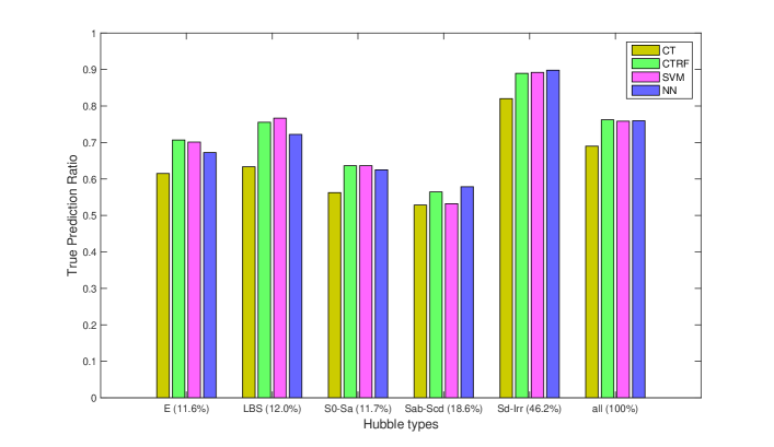
Figure 11: Histograms showing the True Prediction Ratios from panel 1 of Table 3. The different Hubble types in our sample are represented on the x-axis and the TPR values for each type as obtained by the four statistical learning algorithms are shown on the y-axis. The percentage of galaxies of a certain type are shown in brackets next to the Hubble type codes.

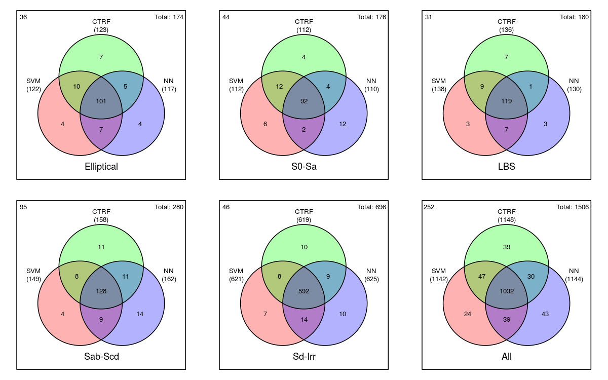
Figure 12: Venn diagrams representing the effectiveness of classification by CTRF, SVM and NN methods for each GAMA Hubble type and over all types. The number of objects ‘correctly’ classified by each method is shown in brackets next to the algorithm labels. The number of objects which were not classified ‘correctly’ by any method is shown in the top left corner while the total number of objects is given in the top right corner.

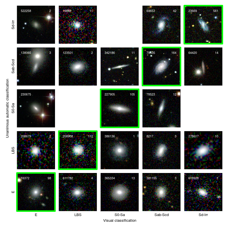
Figure 13: Figure illustrating unanimous disagreement. The x-axis represents the visual classification of the objects while the y-axis shows the unanimous automatic classifications. For example, the galaxy in the bottom most row with ID 611782 has been visually classified as LBS while all four algorithms used in this study classify it as type E. The prime diagonal represents objects for which the visual classification and the four algorithms are in agreement (highlighted in green). The number of objects in each bin is noted in the top right corner of each postage stamp. The other blank spaces denote the absence of objects of x-axis type unanimously classified by the four algorithms as the y-axis type.

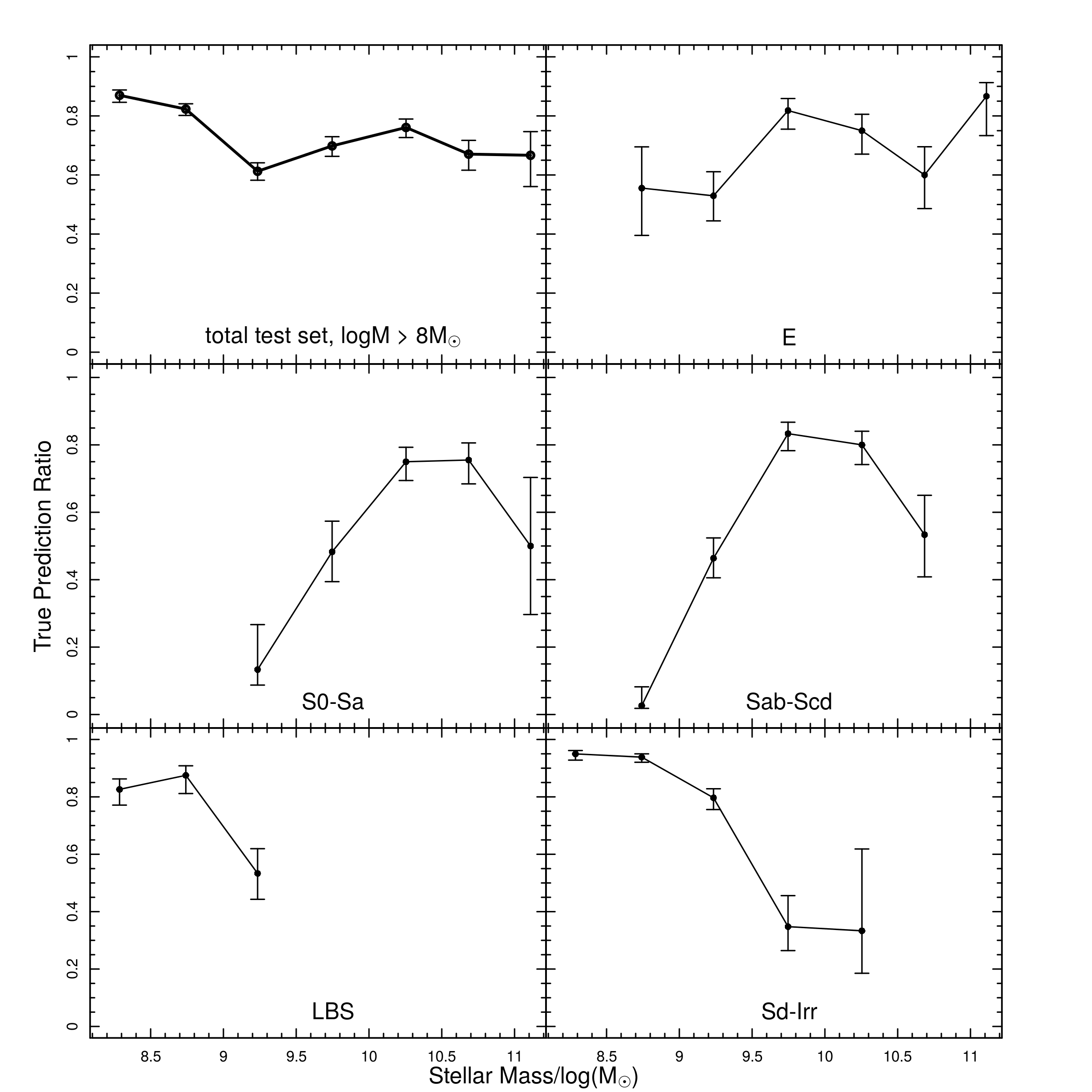
Figure 14: Representation of the TPR as a function of total stellar mass (log) for the method that we recommend, CTRF. The distribution over the total test set is represented in the first panel. The individual contributions of the different GAMA Hubble types are plotted in the subsequent panels as indicated. The lower and upper boundary fractional errors for the data set are calculated by using the aqbeta function from the astro library in R (Cameron, 2011).

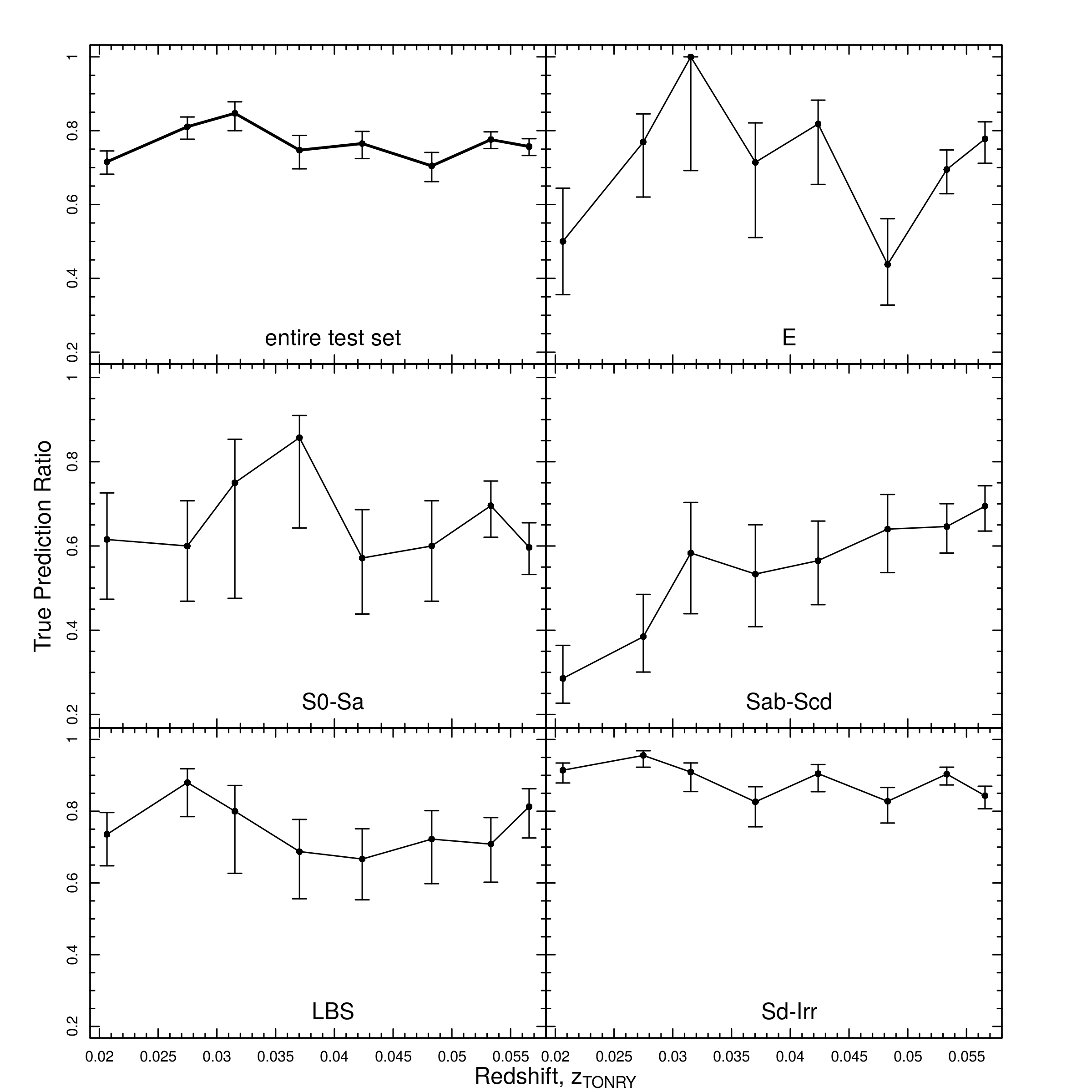
Figure 15: As Figure 14, but as a function of redshift.

The CT, CTRF, SVM and NN codes are run using the parameters shown in Table 2. Figure 11 shows the classification success rate for each morphological type considered in addition to the total sample (‘all’). Galaxy populations are arranged along the x-axis, as indicated. Classification success rate is characterised by the parameter True Prediction Ratio (TPR) shown on the y-axis. TPR (y-axis) represents the quality measure of the classifiers. It is defined as the ratio of the number of correctly classified galaxies to the total number of galaxies considered. The TPR for the machine learning algorithms CT, CTRF, SVM and NN are represented by the colours yellow, green, pink and blue, respectively, for each morphological type. As can be seen, the morphological type Sd-Irr (Type 15) typically returns the highest success ratio at $\sim 90\%$. The morphological type Sab-Scd (Type 1314) returns the lowest average success ratio, typically in the range $\sim 55\%$. Potential reasons for this are discussed in detail in Section 5, but principally revolve around the idea that our algorithms in their current configuration may be more suited to classify single component rather than more complex multi-component systems. The overall average success rate across all morphological types is found to be $\sim 76\%$, with the notable exception of the CT method (see Table 3).

Classification errors can be also characterised using a confusion matrix, $\left(a_{ij}\right)_{i,j=1}^{T}$. The entry of this matrix $a_{ij}$ in the $i$-th row and $j$-th column is the number of galaxies from the class $j$ that are classified as the class $i$ by the classifier.

Note that the above considered quality measure TPR of a classifier for the class $j$ can be calculated using the confusion matrix $\left(a_{ij}\right)_{i,j=1}^{T}$ of this classifier :

$$\mathrm{TPR}_{j}=\frac{a_{jj}}{\sum_{i=1}^{T}a_{ij}}.$$

This quality measure is also known under the names true positive rate or recall.

The TPR of a classifier for all classes is calculated as

$$\mathrm{TPR}_{\mathrm{all}}=\frac{\sum_{j=1}^{T}a_{jj}}{\sum_{i,j=1}^{T}a_{ij}}.$$

In addition to the TPR, another useful characteristic of the classifier performance is the Positive Predictive Value (PPV) or precision. It is calculated for the class $j$ using the confusion matrix $\left(a_{ij}\right)_{i,j=1}^{T}$ :

$$\mathrm{PPV}_{j}=\frac{a_{jj}}{\sum_{i=1}^{T}a_{ji}}.$$

Another important characteristic is the F-score of the classifier. For the class $j$ it is defined as the harmonic mean of $\mathrm{TPR}_{j}$ and $\mathrm{PPV}_{j}$:

$$\mathrm{F}_{j}=\frac{2\cdot\mathrm{TPR}_{j}\cdot\mathrm{PPV}_{j}}{\mathrm{TPR}_{j}+\mathrm{PPV}_{j}}.$$

The confusion matrices and the mentioned performance characteristics of the considered classifiers are presented in Tables 4–8. The actual classification is given in the columns and the classification predicted by the classifiers in rows. The rows and columns represent the five galaxy types.

Visual classification

			E	LBS	S0-Sa	Sab-Scd	Sd-Irr
		E	122	12	35	9	7
		LBS	13	138	3	12	30
		S0-Sa	22	0	112	30	2
		Sab-Scd	10	3	24	149	36
SVM classification		Sd-Irr	7	27	2	80	621

performance characteristics

	E	LBS	S0-Sa	Sab-Scd	Sd-Irr
TPR	70.1	76.7	63.6	53.2	89.2
PPV	66.0	70.4	67.5	67.1	84.3
F	68.0	73.4	65.5	59.4	86.7

Table 4: Confusion matrix and performance characteristics for 5 galaxy classes for the SVM classifier.

Visual classification

			E	LBS	S0-Sa	Sab-Scd	Sd-Irr
		E	107	21	38	11	17
		LBS	4	114	3	8	41
		S0-Sa	37	3	99	34	9
		Sab-Scd	15	9	31	148	58
CT classification		Sd-Irr	11	33	5	79	571

performance characteristics

	E	LBS	S0-Sa	Sab-Scd	Sd-Irr
TPR	61.5	63.3	56.3	52.9	82.0
PPV	55.2	67.1	54.4	56.7	81.7
F	58.2	65.1	55.3	54.7	81.9

Table 5: As for Table 4, but for the CT classifier.

Visual classification

			E	LBS	S0-Sa	Sab-Scd	Sd-Irr
		E	123	15	31	5	11
		LBS	8	136	4	10	31
		S0-Sa	24	1	112	25	2
		Sab-Scd	8	2	26	158	33
CTRF classification		Sd-Irr	11	26	3	82	619

performance characteristics

	E	LBS	S0-Sa	Sab-Scd	Sd-Irr
TPR	70.7	75.6	63.6	56.4	88.9
PPV	66.5	72.0	68.3	69.6	83.5
F	68.5	73.7	65.9	62.3	86.2

Table 6: As for Table 4, but for the CTRF classifier.

Visual classification

			E	LBS	S0-Sa	Sab-Scd	Sd-Irr
		E	117	13	28	7	4
		LBS	9	130	3	11	27
		S0-Sa	27	0	110	23	2
		Sab-Scd	12	3	27	162	38
NN classification		Sd-Irr	9	34	8	77	625

performance characteristics

	E	LBS	S0-Sa	Sab-Scd	Sd-Irr
TPR	67.2	72.2	62.5	57.9	89.8
PPV	69.2	72.2	67.9	66.9	83.0
F	68.2	72.2	65.1	62.1	86.3

Table 7: As for Table 4, but for the NN classifier.

Visual classification

			Spheroid	Disk
		Spheroid	450	73
		Disk	80	903
binary CTRF classification

performance characteristics

	Spheroid	Disk
TPR	84.9	92.5
PPV	86.0	91.9
F	85.5	92.2

Table 8: As for Table 4, but for the binary CTRF classifier.

For Tables 4–7, the left diagonal represents the objects that are correctly classified by the respective classifiers. For.eg., in Table 4, 122, 138, 112, 149 and 621 objects which were visually classified as E, LBS, S0-Sa, Sab-Scd and Sd-Irr were correctly classified by the SVM classifier. The other columns show how many of the objects were classified into which other galaxy types. The same format is followed in all the confusion matrices.

A general trend that is observed for all classifiers is that the ’misclassifications’ by the classifiers are mostly from neighbouring classes. For e.g., in table 4, most of the misclassifications by the SVM classifier of the visual E galaxies are as type S0-Sa. Another interesting inference is that galaxies visually classified as classes LBS and Sd-Irr are frequently confused with each other by all four classifiers. This hints at a possible similarity in properties between these galaxy types.

The confusion matrix of the binary CTRF classifier shown in Table 8 is similar to that of the multi-class classifiers. The actual and predicted classifications are represented by the columns and rows respectively. 450 spheroid-dominated and 903 disk-dominated objects are classified correctly by the binary classifier while the misclassifications are for 80 and 73 objects respectively.

The PPV for the corresponding classes gives a measure of classification error by showing how exact the classifier is. For e.g. in Table 4, in the case of type Sab-Scd, while the SVM classifier only positively classifies $53.2\%$ of the time, there is a probability that when it does, it is $67.1\%$ correct. This measure depends heavily on how balanced the data set is, i.e., if there are more objects of a certain galaxy class in the data sample, that particular galaxy type will have a higher value of PPV. This can be seen clearly in the case of galaxy type Sd-Irr for all the classifiers. It can also be observed in the case of the binary CTRF classifier, for which the data set is more balanced than for multi-class classification, there is a subsequent increase in the PPV of spheroid-dominated objects (which is still the minority class).

The F-score represents the balance between the precision and recall for the classifier. For an unbalanced data set such as ours, the classifier could, in theory, get a higher accuracy rate just by choosing a majority class. In such cases, an F-score is often used to choose an optimum classifier, by choosing one that has consistently high F-scores for all the classes. In the case of the four algorithms considered in this study, that classifier is CTRF as can be seen for both the binary and multi-class classifications.

The CT algorithm is observed to be the lowest grossing method over the entire sample, with an average accuracy of 69.0%. The other three methods, CTRF, SVM and NN have comparable values for classification accuracy at 76.2%, 75.8% and 76.0% respectively. This leads us to conclude that perhaps the choice of parameters is a more important factor in classification accuracy rather than the choice of algorithms. Figure 12 represents the classification efficiencies of these three methods by GAMA Hubble type and for the entire test set. Here, CTRF, SVM and NN algorithms are represented by green, pink and blue respectively. The number of objects that are classified ‘correctly’ by each method is shown in brackets next to the algorithm labels. The number of objects not classified ‘correctly’ by any of the three algorithms is given in the top left corner while the total number of visual Hubble types is given in the top right corner. As can be seen in the case of each individual visual Hubble type and in the total test set (panel 6), the overall performance of the CTRF classifier is slightly better than the other two. Based on these results, we recommend the CTRF classifier for further use in astrophysical practice. Even though the improvement in classification accuracy is marginal, CTRF has a simpler mathematical structure. The CTRF machine learnt classifications will be our primary automatic classifications used for further analysis below.

Figures 2-6 show several example postage stamp images of different galaxy types from our test set. The postage stamps span an area of $3\times$Kron radius of each galaxy and are ordered according to their stellar masses (low-mass galaxies at the top, high-mass galaxies at the bottom). Classifications for different statistical learning algorithms are overlaid on the top right corner of these images in the order SVM, CT, CTRF and NN. As can be seen, the majority of machine learnt classifications agree well with their visual Hubble type, however, there are instances where one or more algorithms classify a galaxy as something different from its visual classification. All four algorithms are in agreement with each other in 1040 out of the 1506 galaxies in our test set. And out of these 1040 objects, 143 (i.e. $\sim 10\%$ of the total test set) differ from the respective visual classification. This ‘unanimous disagreement’ occurs with varying frequency for the different morphological types: $\sim 9\%$ for type E, $\sim 9\%$ for type LBS, $\sim 14\%$ for type S0-Sa, $\sim 21\%$ for type Sab-Scd and $\sim 4\%$ for type Sd-Irr. This phenomenon could be due to two reasons, (1) the visual classification might be inaccurate and, based on the parameters that were used for training, the galaxy belongs to a different class, or, (2) some vital information to classify this galaxy is missing, i.e., the given parameters are not sufficient. Figure 13 shows a few examples of galaxies that exhibit this phenomenon. Further analysis of this interesting occurrence is required to explore why a host of machine learning algorithms may consistently agree with one another yet disagree with the human eye.

4.1 Analysis : CTRF classifier

Figures 14 and 15 represent the TPRs obtained by the CTRF classifier as a function of the total stellar mass and redshift respectively for the galaxies in our test set. In both cases the errors are calculated using the aqbeta function from the astro library in R (Cameron, 2011). This estimates the confidence intervals from quantiles of a beta distribution fit to the data, and is especially suited for small to intermediate data samples.

In Figure 14, the TPRs obtained by the CTRF classifier are plotted against the total stellar masses of the galaxies from our test set. The first panel represents all galaxies while the distributions of distinct GAMA HTs are plotted in the subsequent panels (see legend). We find that the accuracy in classification decreases as the total stellar mass increases. This becomes evident in the extreme mass trends observed for HTs S0-Sa and Sab-Scd. In the case of elliptical galaxies (type 1, E), the TPR values seem to be increasing after a dip at $\log_{10}M_{\odot}\sim 10.5$. This seems to be a real rather than a statistical effect, as the bin centred at $log_{10}M_{\odot}=10.5$ has more objects in it than the one centred at $log_{10}M_{\odot}=11$. For type Sd-Irr, the success rate drops significantly from $\sim 90\%$ at low mass to $\sim 30\%$ at $\log_{10}M_{\odot}>10$. It seems that the algorithm finds it increasingly difficult to classify type Sd-Irr at higher masses, however, we note that the very low number statistics for this population in this mass regime (both in training and test sets), as evidenced by the relatively large error bars could also be a contributing factor. This trend holds true for type LBS as well. Moffett et al. (2016) notes that types LBS and Sd-Irr together account for only about 10% of the total stellar mass density of the parent sample, and that their frequencies drop to nearly zero above the mass range $log_{10}M_{\odot}=10.0$. The reason for the decrease in TPR values in the case of early and intermediate-type spirals isn’t clear at this time, but may be related to the increasingly apparent complexity of structure in galaxies of these types at higher mass regimes.

Figure 15 is a similar representation of the TPRs with the redshifts of all the galaxies in the test set along the x-axis. The first panel represents all the galaxies in our test set while the succeeding panels represent the different HTs (see legend). For the total sample, the trend is to be expected, considering that we have attempted to choose redshift independent parameters. However, we observe varying trends along the sub-populations. The trend for each HT sub-population is similarly consistent with a flat relation with redshift, with the notable exception of type Sab-Scd, for which the TPR is lower at low redshifts and goes on to increase at higher redshifts. This may be due to the fact that local galaxies are better resolved than distant galaxies, and therefore the automated algorithms may be having a harder time processing the extra structural data. The apparent angular scale from $z=0.02$ to $z=0.06$ decreases by a factor of $\sim 3$, which has the effect of blurring stellar populations within the galaxies.

Figures 16-20 show the location of galaxies in the Sérsic index — $g-i$ colour plane with each figure representing a different visual Hubble type morphology. Data point types and colours represent the morphological types assigned to each galaxy by the CTRF classifier. The marginal histograms represent the distributions of $g-i$ colour (top) and Sérsic index (right) for the visual and CTRF classifications. The efficiency of classification by the CTRF classifier for different Hubble types can be visually inspected from these histograms.

Figure 16 shows all visually classified elliptical galaxies in the Sérsic index vs $g-i$ colour plane. Most of the objects for which the classifier is unable reproduce the visual classification are determined to be early-type spirals (S0-Sa). The objects that have been classified by the CTRF classifier as S0-Sa are all redward of the main population, whilst other types are scattered in the blue low Sérsic index tail of the E distribution. One reason for this could be the potential systematic misclassification of face-on red S0 galaxies as ellipticals. If true, our machine learning algorithm may provide a robust automated means by which we could apply corrections to currently existing visual morphological datasets to address the issue of E/S0 confusion. Another reason for this ‘spheroid-disk tension’ between the human eye and the automated algorithms could be the presence of disky elliptical ‘ES’ (Liller 1966; Graham et al. 2016; Savorgnan & Graham 2016) class with intermediate-disks in our sample. It could also be a wider ‘red disk detection’ issue, however, we note that the Sérsic indices for many of these objects are of the order of $n\sim 4$ which indicates spheroid-dominated systems.

Figure 17 shows objects that are visually classified as little blue spheroids (type 2, LBS, represented as green squares). The instances where the CTRF classifier is not in agreement with the visual classifications are represented by the other colours and points in the scatter plot. In general, most of the objects which were not found to be LBS by the CTRF method have been classified as late-type spirals & irregulars, except towards the redder end of the scatter plot, where they have been classified as elliptical galaxies. We note that in the visual classification of this particular type, the ‘blue colour’ was a secondary characteristic, the objects were primarily classified on the basis of their shape and size.

Figure 18 shows objects visually classified as early-type spiral galaxies (type 1112, S0-Sa, barred and unbarred, represented as black diamonds). The CTRF classifier’s classifications that do not agree with the visual morphology are almost equally divided between ellipticals (red circles) and intermediate-type spirals (purple triangles). They seem to be uniformly distributed in Sersic index space, while there appears to be some dependence in $g-i$ colour, with the objects classified as ellipticals clustered in an area redder than the objects that are classified as intermediate-type spirals. Classification as intermediate-type spiral follows a trend observed by Owens et al. (1996), in that differentiating between neighbouring classes of galaxies such as these is more difficult than differentiating between non-neighbouring classes. The population of elliptical galaxies we find might be an indicator that the human eye is fallible when classifying this type of galaxy. Very few objects are classified as late-type spirals & irregulars or little blue spheroids (mostly at the bluer end).

Figure 19 shows objects that are visually classified as intermediate-type spirals (type 1314, Sab-Scd, purple triangles). In most instances where the CTRF classifier disagrees with the visual classification, it classifies objects as late-type spirals & irregulars. However, at the redder and higher Sérsic index end, some objects are classified as early-type spirals. This is also the galaxy type for which the classifiers of the machine learning algorithms that we have applied disagree the most with visual classifications.

Figure 20 shows objects that are visually classified as late-type spirals & irregulars (type 15, Sd-Irr, represented as blue triangles pointing down). For this particular galaxy type, all four machine learning algorithms have a high agreement rate with the visual classifications ($>80\%$). As is shown, the disagreements are evenly divided between types LBS and intermediate-type spirals, while there are a few objects classified as ellipticals. The classifications as LBS and ellipticals could be an indication that these objects may have more in common with early-type galaxies than is currently conceived. The classifications as intermediate-type spirals are likely due to the Owens et al. (1996) observations mentioned previously.

4.2 Impact of chosen parameters on the CTRF classifier

Table 9: Results of parameter sensitivity test on the CTRF algorithm in percentages are shown in panel 1. In panel 2 similar results for redundant parameters according to the PCA performed in Section 2.4 (Figure 1) are shown. The results for the CTRF classifier from the original run are shown in panel 3.

Parameter removed	E 1	LBS 2	S0-Sa 1112	Sab-Scd 1314	Sd-Irr 15	All
Sérsic index	67.8	76.7	58.5	55.7	87.9	74.8
Kron radius in kpc (semi-minor axis)	69.0	71.7	62.5	55.7	88.7	75.2
Half-light radius in kpc	65.5	68.9	60.8	56.8	90.5	75.3
Kron radius in kpc (semi-major axis)	67.8	70.6	61.4	56.8	89.8	75.5
Ellipticity	66.7	74.4	63.1	57.1	88.8	75.6
Mass-to-light ratio	69.5	71.7	62.5	57.5	89.1	75.8
$g-i$ colour	67.2	76.7	63.6	56.4	88.8	76.0
Stellar mass	70.7	71.7	64.2	57.5	88.8	76.0
$u-r$ colour	70.7	74.4	62.5	56.8	89.0	76.0
Absolute magnitude	71.8	73.3	61.4	58.2	90.0	76.5
Mass-to-light ratio & $g-i$ colour	68.4	75.0	63.7	60.0	89.1	76.6
Mass-to-light ratio & $u-r$ colour	67.8	75.6	60.8	57.9	89.7	76.2
$u-r$ colour & $g-i$ colour	69.5	76.1	61.4	60.4	89.4	76.8
All chosen parameters	$70.7^{+3.2}_{-3.7}$	$75.6^{+2.9}_{-3.5}$	$63.6^{+3.5}_{-3.8}$	$56.4^{+2.9}_{-3.0}$	$88.9^{+1.1}_{-1.3}$	$76.2^{+1.1}_{-1.1}$

We perform a sensitivity test to ascertain the impact of each parameter on the classification process of our CTRF algorithm. In order to achieve this, we remove all the parameters mentioned in the upper panel of Table 2 one by one, and obtain the TPRs, re-training the CTRF classifier in each instance. The results of this are shown in Table 9.

The removal of Sérsic index lowers the overall rate of accuracy the most, by almost $1.4\%$. All other increases and decreases from the overall TPR caused by the removal of parameters are within the error limits defined in Table 3. The only parameter whose removal causes an increase in the overall TPR is absolute magnitude, by $0.3\%$. This indicates that for the total data sample, Sérsic index is the parameter that contributes most to the classification process by the CTRF algorithm. This, however, does not hold true for the individual Hubble types.

Removal of $u-r$ colour and stellar mass does not affect the classification in the case of elliptical galaxies. Absolute magnitude and mass-to-light ratio have an almost similar effect on the TPR values, albeit in different directions. When absolute magnitude is removed, the TPR value increases by $1.1\%$ and when mass-to-light ratio is removed, the value decreases by $1.2\%$. The parameters for which the accuracy falls outside the error bars are ellipticity and half-light radius.

In the case of LBS galaxies, the parameters that affect the classification process the most are half-light radius, Kron radius (semi-major and semi-minor), mass-to-light ratio and stellar mass. The parameters that have a similar effect on the classification rate are Kron radius (semi-minor axis), mass-to-light ratio and stellar mass, a decrease by $\sim 4\%$. The decrease in TPR values is drastic in the case of both half-light radius and Kron radius (semi-major axis), $\sim 7\%$ and $\sim 5\%$ respectively.

For early-type spiral galaxies, the changes in TPR are within the error bars except in the case of Sérsic index. When Sérsic index is removed prior to training the classifier, the accuracy drops by $\sim 5\%$. The effects caused by the absence of Kron radius (semi-minor), mass-to-light ratio and $u-r$ colour are analogous, a decrease of $\sim 1\%$. Same is the case with Kron radius (semi-major) and absolute magnitude, by $\sim 2\%$. When $g-i$ colour is excluded from the process, the TPR values remain the same as that from the original run.

The change in accuracy for intermediate-type spirals after removing the parameters one by one, are all within the error limits of the values from Table 3. As in the case of early-type spirals, removing $g-i$ colour has no effect on the original TPR values. Sérsic index and Kron radius (semi-minor) contribute to a decrease in TPR values by $\sim 0.7\%$ each; Kron radius (semi-major), half-light radius and $u-r$ colour to an increase by $\sim 0.4\%$ each; and mass-to-light ratio and stellar mass to an increase by $\sim 1\%$ each. Removing absolute magnitude seems to matter the most, by increasing the accuracy by $\sim 2\%$.

The changes in TPR in the case of late-type spirals & irregulars are mostly within the error bars of the original results, except in the case of half-light radius where it increases by $\sim 2\%$, which seems to have the most impact on classification accuracy as well. Ellipticity, $g-i$ colour and stellar mass have a similar effect on the TPR values (decrease by $0.1\%$). $u-r$ colour seems to have a similar impact on the classifier’s performance for this galaxy class, an increase of the TPR by $0.1\%$.

In the PCA we performed (represented in Figure 1), ellipticity was found to be the parameter which contained the least variability. But as can be seen from Table 9, while it might not be the most important parameter overall, it has a significant impact in the classification accuracies of individual Hubble types, especially elliptical galaxies. The TPR of ellipticals fall by $4\%$ when this parameter is removed.

Also represented in Figure 1 is the redundancy of the parameters, mass-to-light ratio, $g-i$ and $u-r$ colours. We also explore here, the impact on the classification accuracies when these parameters are removed two at a time.These results are represented in the second panel of Table 9.

When mass-to-light ratio and $g-i$ colour are removed, there is a marginal increase in the overall TPR value, to $76.6\%$. This increase is reflected in the individual Hubble types, S0-Sa, Sab-Scd and Sd-Irr. The accuracies take a consequent dip in the case of types E and LBS.

The removal of mass-to-light ratio and $u-r$ colour does not make a significant overall impact, with the TPR value remaining the same as that of the original run, at $76.2\%$. Among the individual Hubble types, the accuracy of LBS remains unchanged while that of types E and S0-Sa decrease. The individual TPRs of types Sab-Scd and Sd-Irr reflect marginal increases.

Removing $g-i$ and $u-r$ colours resulted in an increase in the overall TPR value, to $76.8\%$. This increase was contributed by the increases in the TPRs of galaxy types LBS, Sab-Scd and Sd-Irr. The accuracies of types E and S0-Sa was found to drop marginally.

The slight increases and decreases in the TPR values when the parameters are removed one by one are largely within the error margins defined for the TPRs from the original run and therefore are not deemed significant. Similar is the case when redundancies in parameters are removed. Therefore we conclude that, while the individual Hubble types might be sensitive to certain parameters more than the others, all parameters contribute to some extent in the overall classification process of the CTRF algorithm.

4.3 CTRF classifier for binary classification

Table 10: Panel 1 shows the results of parameter sensitivity test performed with the binary CTRF classifier. The results with all chosen parameters (Table 2) are shown in panel 2.

Parameter removed	Spheroid -dominated	Disk -dominated	All
Half-light radius in kpc	78.7	92.1	87.4
Sérsic index	82.5	90.4	87.6
Kron radius in kpc (semi-major axis)	82.6	91.4	88.3
Kron radius in kpc (semi-minor axis)	83.8	91.2	88.6
Mass-to-light ratio	83.6	91.4	88.7
Stellar mass	83.0	92.0	88.8
Ellipticity	84.9	91.3	89.0
$g-i$ colour	84.3	91.6	89.0
Absolute magnitude	84.8	91.6	89.2
$u-r$ colour	83.8	92.1	89.2
All chosen parameters	$84.9^{+1.4}_{-1.7}$	$92.5^{+0.8}_{-0.9}$	$89.8^{+0.7}_{-0.8}$

With the same training, test and parameter sets that we have employed in multi-class classification, we constructed a binary CTRF classifier with two classes, spheroid-dominated and disk-dominated. The galaxies which were visually classified as ellipticals (type 1, E), little blue spheroids (type 2, LBS) and early-type spirals (type 1112, S0-Sa) were considered as spheroid-dominated while the intermediate-type spirals (type 1314, Sab-Scd) and late-type spirals & irregulars (type 15, Sd-Irr) were considered as disk-dominated.

This binary CTRF classifier returned a total success ratio of $89.8\%^{+0.7}_{-0.8}$ with individual TPRs of $84.9\%^{+1.4}_{-1.7}$ and $92.5\%^{+0.8}_{-0.9}$ for the spheroid-dominated and disk-dominated classes respectively. This significant increase from the original CTRF classifier’s TPRs proves that as the number of classes into which classification is made increases, the classification accuracy decreases. This might also be directly related to the size of the data set, and how well each class is represented in the training set.

Similar to the analysis in Section 4.2, we also explored the impact the different parameters might have on the classification performance of the classifier constructed by the CTRF algorithm. The results of this are given in Table 10.

Removing half-light radius from the parameter set used for training and testing the CTRF algorithm seems to be the have the most impact on the performance of the binary CTRF classifier. While the overall success rate drops by $2.46\%$, the values for spheroid-dominated and disk-dominated systems fall by $\sim 6\%$ and $\sim 0.4\%$ respectively. This points at the greater significance of half-light radius in the classification of spheroid-dominated galaxies rather than the disk-dominated ones. This is in agreement with the results represented in Table 9 in which the classification accuracies fall consistently for these three classes (E, LBS and S0-Sa) in the case of multi-class classification.

Ellipticity & $g-i$ colour and absolute magnitude & $u-r$ colour seem to have similar overall effect on the classification process, drops by $\sim 0.8\%$ and $\sim 0.6\%$ for the respective pairs. The fluctuations in the TPR values are most significant in the case of ellipticity for disk-dominated systems. The entire contribution to the change in TPR while ellipticity is removed as a classifying criterion comes from disk dominated systems. This is a very interesting development because, in the case of multi-class CTRF classification discussed in Section 4.2, ellipticity is one of the parameters that cause the TPR to decrease for all three galaxy types collectively called as spheroid-dominated. This might indicate cross-contamination between these three galaxy types in the visually classified sample which confuses the classifier.

The accuracy rates (both overall and individual) fall beyond the error margins when parameters such as Sérsic index, Kron radii (major and minor axes), mass-to-light ratios and stellar mass are removed. According to this study, the parameters that influence our CTRF algorithm the most are half-light radius, Sérsic index, Kron radii, mass-to-light ratio and stellar mass.

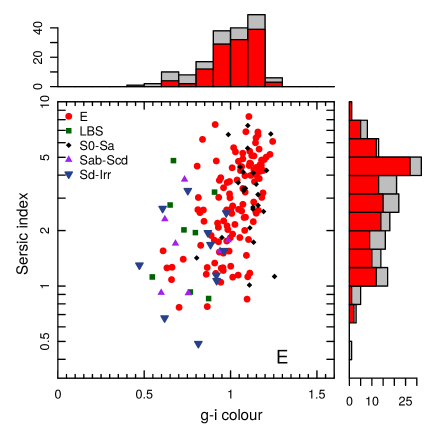
Figure 16: Scatter plot with marginal histograms showing all visually classified elliptical (type 1 , E) galaxies in Sérsic index and $g-i$ colour space. Data point colours and types vary according to their CTRF classification, as indicated by the inset legend. Marginal histograms show the distribution for all (grey) and visually classified elliptical (red) galaxies.

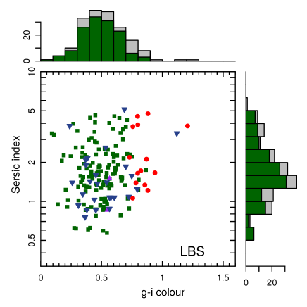
Figure 17: As Figure 16, for Little Blue Spheroids (type 2, LBS).

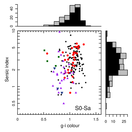
Figure 18: As Figure 16, for early type spirals (type 1112, S0-Sa, barred and unbarred).

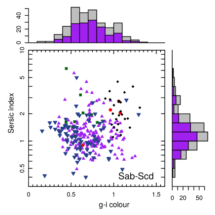
Figure 19: As Figure 16, for intermediate type spirals (type 1314, Sab-Scd, barred and unbarred).

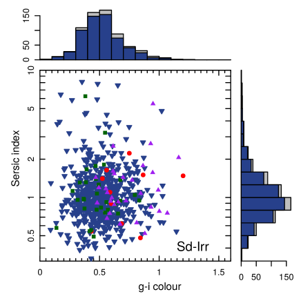
Figure 20: As Figure 16, for late type spirals & irregulars (type 15, Sd-Irr).

5 Discussion

Table 11: Summary of the results from this study (top) alongside results from several other studies from the literature using a variety of statistical learning methods (bottom).

Statistical Learning Method	Total sample	Training set	Test set	Number of classes	Dimensions	Accuracy	Reference
}1020pt					{1020pt
SVM						75.8%
	7528	6022 (80%)	1506 (20%)	5	10
NN						76.0%	Results from our work
CT						69.0%
CTRF						76.2%
SVM	$\sim 1500$	500 (33%)	1000 (67%)	2 (early-type, late-type)	12	80%	Huertas-Company et al. (2007)
NN	$\sim$1,000,000	$\sim$75,000 (7.5%)	$\sim$925,000 (92.5%)	3 (early-type, spirals, point sources/artefacts)	12	90%	Banerji et al. (2010)
Oblique CT	5217	$\sim$4174 (80%)	$\sim$1043 (20%)	5 (E, S0, Sa+Sb, Sc+Sd, Irr)	13	63%	Owens et al. (1996)
Three CT algorithms including CTRF	75,000	67,500 (90%)	7500 (10%)	3 (ellipticals, spirals, unknown)	13	96.2%	Gauci et al. (2010)
ConvNet	58,000	47,700 ($\sim 82\%$)	5000 ($\sim 9\%$)	5 (probablities†)	run on images	$\sim$99%	Huertas-Company et al. (2015)
			5300 ($\sim$9%) used for real-time evaluation during training				Dieleman et al. (2015)

^†Probabilities for each galaxy having a disk or a spheroid, being a point source, having an irregularity or being unclassifiable are the outputs.

In this section, we discuss in greater detail our previously recovered results. To begin, we note that type 15 (Sd-Irr galaxies), account for almost 50% of our test set, and the associated TPR success values are above 80% for all considered automated classification methods. This could indicate one of three scenarios; (1) As the percentage of objects in a certain class increases, the accuracy of classification increases as well, (2) the algorithms that we tested are more effective in classifying a particular Hubble type (type 15 in our case) using the parameters that we have prescribed or (3) the human classifications may be biased towards being able to more accurately classify Sd-Irr type galaxies.

The first scenario is not generally supported by our own results. The TPR values for type 1314 are consistently low across all 4 considered methods and yet it is the second most populous type in both our training and test sets. This warrants additional analysis in future works; by testing the codes on larger data samples and by fine-tuning the classification algorithms by introducing techniques such as cross-validation.

As to the second scenario, the successful utilisation of our adopted functions are directly linked to our choice of parameters. It may be that one or more of the parameters that we have chosen are more effective in classifying certain Hubble types while falling short in others. For example, the complexity in the structure of the galaxy might not be well defined by the parameters that we have chosen. As can be seen in Table 3, the TPR values are considerably higher for single component systems such as ellipticals (type 1, E) and late-type spirals/Irregulars (type 15, Sd-Irr) compared to multi-component systems such as early and intermediate type spirals (types 1112, S0-Sa and 1314, Sab-Scd respectively).

All four algorithms are in agreement with each other in 1040 out of the 1506 galaxies in our test set. And out of these 1040 objects, 143 (i.e. $\sim 10\%$ of the total test set) disagree with the classification by visual inspection. Of these, $\sim 9\%$ are ellipticals, $\sim 9\%$ are LBS, $\sim 14\%$ are early-type spirals, $\sim 21\%$ are intermediate-type spirals and $\sim 4\%$ are late-type spirals & irregulars. These are illustrated in Figure 13. There seems to be an element of symmetry in this occurrence. For instance, as can be seen from the figure, no objects that have been visually classified as S0-Sa are machine classified unanimously as Sd-Irr, this pattern holds true in converse as well. But this isn’t always the case. No visual LBS galaxies have been unanimously machine classified as S0-Sa objects but one visual S0-Sa galaxy has been machine classified unanimously as LBS. This, along with the possibility of unanimous disagreement being a potential indicator of human error in classification by visual inspection are interesting paths to follow in future works that extend this study.

When we train a machine, for e.g., to classify galaxies (our case) based on visual classifications, what we essentially do is train it to reproduce our classification strategy, replete with our human biases. For instance, if, beyond a certain redshift, the human eye is ineffective in distinguishing between certain classes of galaxies, the data set that we apply to the algorithms will reflect the same bias. Therefore, we propose that the disagreement between the machine and the visual classifications could be due to one of two reasons, (1) the visual classification is inaccurate, and based on the values of the parameters used to train and test the algorithms, the galaxy belongs to one of the other classes, or (2) the parameters do not sufficiently characterise what we see while classifying by eye.

In Figures 16, 17 and 20 it can be seen that the CTRF method replicates the visual classification to a greater extent than in Figures 18 and 19. This leads us to speculate that our algorithms in their present configuration might be more effective in classifying single component systems such as ellipticals and late-type spirals rather than multi-component systems like early and intermediate-type spirals.

One of the methods that we have used in our work is SVM with a tree structure. With this approach, the accuracy obtained on our entire test set is 75.8%. The accuracies for the different HTs are represented in Table 3. This value seems encouraging when we compare our results to Huertas-Company et al. (2007), who also used an SVM approach in their work to obtain morphological classification to a sample of 1500 galaxies from the SDSS (500 to train, 1000 to test). Their method was a generalisation of C-A system using non linear SVM boundaries with 12 dimensions. The mean accuracy of the method was $\sim 80$%. We note that the Huertas-Company et al. (2007) method only classifies galaxies into early and late types while our algorithm classifies galaxies into five distinct morphological types, which may explain why their success ratio is $\sim 4\%$ higher than ours.

In our NN method, we reproduce the classifications learned on the training set to an accuracy of 76.0% on the test set. Banerji et al. (2010) applied artificial neural networks to a sample of almost one million objects from the SDSS previously classified by human eye by volunteers as part of the Galaxy Zoo project. Their training set consisted of 75000 objects, classifying the test set into three morphological classes (early-types, spirals and point sources/artefacts) with 12 parameters. The accuracy of their approach was close to 90%. Considering that our training set and test sets are much smaller compared to Banerji et al. (2010) and that we use a larger range of classification types, our value of 76.0% is highly promising.

Our CT algorithm uses classification (decision) trees to attain morphological classification with an accuracy of 69.0% on our entire test set. The size of the data set and the number of classification types for the method of Owens et al. (1996) is comparable to our own. They use a sample of 5217 galaxies from the ESO-LV catalogue (Lauberts & Valentijn, 1989) using 13 parameters to discern between five morphological types (ellipticals, lenticulars, early-type spirals, late-type spirals and Irregulars). With a five-fold cross validation on their approach they achieved an average accuracy of 63% on a test set which amounted to 1/5th of the whole set. They have compared their results with Storrie-Lombardi et al. (1992) which applied an artificial neural network approach to the same data with an accuracy of 64.1% and Lauberts & Valentijn (1989) whose automated classifier reproduced classifications to an accuracy of 56.3%. We note however, that Storrie-Lombardi et al. (1992) have used $\sim 30\%$ of their total data sample as the training set and  70% as the test set in contrast to our method of adopting a larger training set and smaller test set as detailed in Section 2.5. The improvement of 69.0% accuracy that we observe is undoubtedly due to this reason. Furthermore, we have  2000 more objects in the data sample which will influence the classification accuracy.

Among our methods the CTRF algorithm which employs a random forest of 100 trees was found to have an accuracy of 76.2%. This method has a marginal but encouraging higher accuracy among all four methods that we have tested. Gauci et al. (2010) performed a comparison of different classification tree algorithms to a data set of 75000 objects from the SDSS previously classified by the Galaxy Zoo project. The algorithms of CART, C4.5 and Random Forest (RF) are tested with a ten-fold cross validation technique where, in each run, nine subsets of the data are used for training and one for testing. The success rate was 97.33% for an RF algorithm with 50 trees and 96.2% over all the methods. However, Gauci et al. (2010) have only 3 classification types (elliptical, spiral and unknown morphology) compared with 5 in this study.

We trained a binary CTRF classifier that classifies our data sample to spheroid-dominated and disk-dominated systems. For this, we consider galaxy types E, LBS and S0-Sa as spheroid-dominated and galaxy types Sab-Scd and Sd-Irr as disk-dominated. The overall accuracy rate for this classifier is $\sim 90\%$ with individual TPRs for spheroid-dominated and disk-dominated systems to be $\sim 85\%$ and $\sim 93\%$ respectively.

The results from our binary CTRF classifier has clarified certain aspects about the effectiveness of our overall study. The results indicate that the number of data types into which the classification is done is a very important criterion for accuracy. There is an increase of almost $14\%$ overall accuracy when the number of types changed from 5 to 2. It is conceivable that the size of the data set and how comprehensively the different galaxy types are represented in the training and test sets play a role in the performance accuracy as well. This can be seen in the higher accuracy of the disk-dominated galaxies which make up $\sim 67\%$ of the total data set. So a way to address the decrease in accuracy as the galaxy types increase might be to increase the size of the data set accordingly.

To facilitate future studies and to aid in comparison with other works (see Table 11), the machine learning algorithms employed in this study have not been significantly modified beyond their default setups as detailed in Section 3. There are several avenues that could be pursued in order to make them more precise. Applying the SVM method for multi-class classification using error-correcting output codes is one such approach (Dietterich & Bakiri 1995). There are indications in literature that this technique could be more accurate than the tree structure that we have considered in this work. Assigning probabilities to our classifications rather than binary values may be a useful tool to see the effectiveness of the classification process. Owens et al. (1996) posits that differentiating between neighbouring classes of galaxies (for e.g., types 1112 and 1314 in our sample) is more complicated than differentiating between non-neighbouring classes of galaxies. By analysing the probabilities assigned to each class by the classification algorithms and manual examination, it might be possible to define criteria or introduce parameters that provide a more robust delineation between neighbouring galaxy types. Introducing Principal Component Analysis (PCA) as a means to choose a robust set of parameters and extensive error analysis of the parameters that we have chosen are other interesting prospects, allowing for the introduction (e.g. some measure of asymmetry) or elimination of parameters (e.g. ellipticity) which do not seem to be vital in predicting morphology. The methods that we have chosen construct classifiers with different mathematical structures.Therefore each constructed classifier may capture different aspects of the ideal classifier effectively. Using a combination of classifiers constructed using different statistical learning methods may give rise to a new classifier with better accuracy (and closer to an ideal classifier) than each classifier taken individually (Chen et al. 2015; Kriukova et al. 2016). The design of appropriate combination strategies is another avenue that we may explore in the future.

6 Conclusion

In this study, we have used the statistical machine learning algorithms of Support Vector Machines (SVM), Classification Trees (CT), Classification Trees with Random Forests (CTRF) and Neural Networks (NN) to carry out morphological classifications for 7528 galaxies from the Galaxy and Mass Assembly (GAMA) survey. These galaxies were previously visually classified independently by three classifier teams and the majority vote has been included in the GAMA catalogue. The algorithms are trained on a set of 6022 objects (80% of the data set) using 10 distance independent parameters. These algorithms are subsequently tested on the remaining 20% of the data set (1506 objects) to classify them into five galaxy types: elliptical (type 1, E), little blue spheroid (type 2, LBS), early-type spirals (type 1112, S0-SBa), intermediate-type spirals (type 1314, Sab-SBcd) and late-type spirals & irregulars (type 15, Sd-Irr). We draw the following conclusions from our study.

1. [i]

2. The success rates on the entire test set are 69.0%, 76.2%, 75.8% and 76.0% for the CT, CTRF, SVM and NN algorithms respectively. While the performance of the SVM, CTRF and NN algorithms are very similar, the CTRF algorithm has a marginally better success rate and a simpler mathematical structure. We therefore recommend this algorithm to provide robust, automated Hubble type classifications when applied to future extragalactic surveys.

3. Our algorithms have a greater success rate in the case of single component systems such as ellipticals, late-type spirals & irregular galaxies. This is especially clear when we look at the success rate of type 15 galaxies (Sd-Irr). They form 47% of our entire sample. The success rates of all four algorithms are above 80% for this galaxy type and close to 90% for CTRF, SVM and NN algorithms.

4. We find that the success rates decrease with increasing stellar mass. This trend seems drastic in the case of HTs S0-Sa, Sab-Scd and Sd-Irr. This apparent phenomenon warrants further investigation.

5. We do not find a universal trend in the success rates with respect to redshift, however, we find that there is some redshift dependence within each galaxy type. This is especially apparent in the case of type Sab-Scd, for which, the success rates are lower at lower redshifts and increase towards higher redshifts.

6. In the cases where all 4 machine learning algorithms agree with each other, they disagree with the visual classification $\sim 10\%$ of the time, with $\sim 9\%$ being ellipticals, $\sim 9\%$ LBS, $\sim 14\%$ S0-Sa, $\sim 21\%$ Sab-Scd and $\sim 4\%$ Sd-Irr. These unanimous disagreement fractions could be a potential indicator for human error in visual classifications. Further exploration of this is an interesting path to investigate for future work.

7. When we decrease the number of galaxy types into which classification is done, the accuracy of classification increases considerably. Our binary CTRF classifier achieved an overall accuracy of $89.8\%$ with the spheroid-dominated and disk-dominated classes achieving accuracies of $84.9\%$ and $92.5\%$ respectively. This hints that a way to cope with the decrease in classification accuracy as the galaxy types increase might be to use larger data sets.

8. There are many possible avenues to pursue following from this study. These include introducing analysis methods such as PCA or cross-validation to create a robust dataset of input features, foregoing the SVM tree structure in favour of error-correcting codes, and using an ensemble of classifiers constructed using different statistical learning methods.

Appendix A Appendix : Methods in detail

A.1 Support Vector Machines

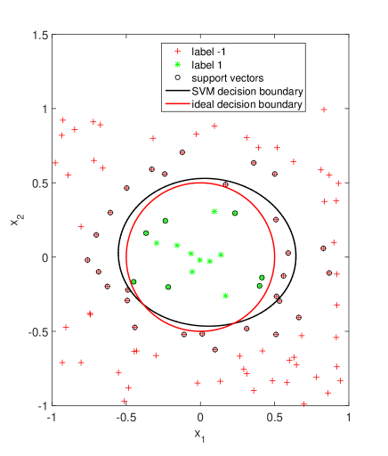
Figure 21: Illustrative example for the SVM method in the case of two features $x_{1},x_{2}$. The feature vector belongs to the class $1$ if it is inside the red curve, which is the ideal decision boundary. Otherwise, the feature vector is in the class $-1$. The black curve is the decision boundary constructed by the SVM method using the training data in the picture. The corresponding constructed SVM classifier assigns the feature vectors inside this black curve to class $1$, and outside the black curve to class $-1$. The training feature vectors that are additionally marked by a small surrounding circle are the support vectors.

In SVM, the constructed classifier $f$ is of the following form:

$$f\left(\mathbf{x}\right)=\operatorname{sign}\left(g\left(\mathbf{x}\right)\right)=\operatorname{sign}\left(b+\sum\limits_{i=1}^{N}\alpha_{i}K\left(\mathbf{x},\mathbf{x}_{i}\right)\right)$$ (1)

where $K$ is a positive definite kernel, and $b,\alpha_{i},\;i=1,2,\dots,N$ are certain coefficients from ${\mathbb{R}}$. We set $\boldsymbol{\alpha}:=\left(\alpha_{1},\alpha_{2},\dots,\alpha_{N}\right)^{\top}$.

The coefficients $b$, $\boldsymbol{\alpha}$ are chosen as the solution of the following minimisation problem:

$$\sum\limits_{i=1}^{N}\left(1-z_{i}g\left(\mathbf{x}_{i}\right)\right)_{+}+\frac{\lambda}{2}\boldsymbol{\alpha}^{\top}\mathbf{K}\boldsymbol{\alpha}\longrightarrow\min\limits_{b,\boldsymbol{\alpha}},$$ (2)

where $(a)_{+}:=\max(0,a)$, $\mathbf{K}$ is the $N\times N$ kernel matrix with entries $\mathbf{K}_{ij}=K\left(\mathbf{x}_{i},\mathbf{x}_{j}\right)$, and $\lambda>0$ is a penalty parameter. Note that the minimisation problem in Equation (2) is convex, and therefore, various methods of convex optimisation (e.g., Boyd & Vandenberghe 2004) can be used to solve it. We employ the sequential minimal optimisation method, which is suggested in MATLAB as the standard method to solve this. The first term in Equation (2) measures the closeness of $f\left(\mathbf{x}_{i}\right)=\operatorname{sign}\left(g\left(\mathbf{x}_{i}\right)\right)$ to $z_{i}$, i.e. it tells us how well the classification is predicted on the training set, while the second term penalises coefficients in $\boldsymbol{\alpha}$, and $\lambda$ gives a tradeoff between the two terms. We take the default value for $\lambda$, which is $\lambda=1$.

Due to the nature of the function $(\cdot)_{+}$ in Equation (2), many values of $\alpha_{i}$ are equal to $0$. Therefore, in the representation in Equation (1), the linear combination involves functions from a subset of $\Set{K\left(\cdot,\mathbf{x}_{i}\right),\;i=1,2,\dots,N}$, and the corresponding $\mathbf{x}_{i}$ are called support vectors.

The kernel that we have chosen is the Gaussian Radial Basis Function given as:

$$K\left(\mathbf{x},\mathbf{x}^{\prime}\right)=\exp\left(-\frac{\left\|\mathbf{x}-\mathbf{x}^{\prime}\right\|^{2}}{2\sigma^{2}}\right),$$ (3)

where $\sigma$ is the scaling factor, whose default value we have retained as $\sigma=1$.

The SVM method is illustrated by an example in Figure 21. In this example, the feature vector is $\left(x_{1},x_{2}\right)\in[-1,1]\times[-1,1]$ and $D:=\Set{\left(x_{1},x_{2}\right)}{x_{1}^{2}+x_{2}^{2}\leq\left(1/2\right)^{2}}$ is a disk with its centre as $(0,0)$ and radius $1/2$. The ideal classifier $f^{*}$ assigns the feature vector to class $1$ if it belongs to $D$, and to class $-1$ otherwise. We generate a training set $\mathcal{Z}$ that consists of $100$ feature vectors $\mathbf{x}_{i}=\left(x_{1,i},x_{2,i}\right)$. Features $x_{1,i}$, $x_{2,i}$ are randomly sampled using the uniform distribution over $[-1,1]$. The classes for the feature vectors $\mathbf{x}_{i}$ in the training set are determined using the ideal classifier $f^{*}$. Then, we construct the function $g$ using the described SVM method with kernel Equation (3) and $\sigma=1$.

The red curve is the boundary of $D$, which can be called as the ideal decision boundary. The black curve consists of feature vectors $\mathbf{x}$ for which $g(\mathbf{x})=0$. This curve is called the SVM decision boundary. For the feature vectors inside this curve, we have $g(\mathbf{x})>0$, and therefore, these feature vectors will be classified by the constructed SVM classifier $f$ as class $1$. The other feature vectors satisfy the condition $g(\mathbf{x})<0$, and therefore, they are assigned by $f$ to class $-1$. The training feature vectors inside the small circles are the support vectors.

In general, the SVM decision boundary may have an arbitrary shape, and it may also consist of several closed curves. The support vectors are located near the SVM decision boundary, in a way supporting and defining its shape.

A.2 Classification Trees with hyper-rectangular partitions

In the CT method, the feature space is split into the rectangular partitions by a recursive binary method. First, it is split into two regions, $\Set{\mathbf{x}\in{\mathbb{R}}^{p}}{x_{i}<s}$ and $\Set{\mathbf{x}\in{\mathbb{R}}^{p}}{x_{i}\geq s}$ using a selected feature $x_{i}$ and a split point $s$. Then, one or both of these regions are split similarly into two more regions. this process continues until a certain stopping condition is fulfilled.

An example of the above described partition for two features $\left(x_{1},x_{2}\right)$ with values in the unit square is presented in Figure 8. In this example, the first split is made at $x_{1}=s_{1}$. Then, the region $\Set{\mathbf{x}\in{\mathbb{R}}^{p}}{x_{1}<s_{1}}$ is split at $x_{2}=s_{2}$, and the region $\Set{\mathbf{x}\in{\mathbb{R}}^{p}}{x_{1}\geq s_{1}}$ at $x_{1}=s_{3}$. In the end, the region $\Set{\mathbf{x}\in{\mathbb{R}}^{p}}{x_{1}\geq s_{3}}$ is split at $x_{2}=s_{4}$. Thus the partition of the feature space into five rectangular regions $R_{1}$, $R_{2}$, $\dots,$ $R_{5}$ shown in Figure 8 is obtained.

The nodes of the CT are split based on the impurity measure of the node. We represent the region that corresponds to the node $t$ as $R_{t}$. Let $N_{t}:=\#\Set{\mathbf{x}_{i}\in R_{t}}$ denote the number of training feature vectors in $R_{t}$. The mathematical notation $\#R$ is used for the number of elements of a set $R$. We further define $p_{k}(t):=\#\Set{\mathbf{x}_{i}\in R_{t}}{y_{i}=k}/N_{t}$ as the proportion of the training feature vectors in the node $t$ (or, which is the same, in the region $R_{t}$) that belong to class $k$. Impurity measure $I(t)$ of the node $t$ is a function of the proportions $p_{k}(t)$. It tells us how even the distribution of the feature vectors in the node $t$ are over the classes. It has a maximum value when the feature vectors are distributed evenly over the classes in the node $t$, i.e. when $p_{k}(t)=1/T$, $k=1,2,\dots,K$. In contrast, when the node $t$ contains feature vectors only from one class, say class $\ell$, i.e. when $p_{\ell}(t)=1$, and $p_{k}(t)=0$, $k\neq\ell$, then the impurity measure $I(t)$ has a minimal value, and the node is called pure. As the impurity measure, we consider the Gini index : $I(t)=1-\sum_{k=1}^{T}p_{k}^{2}(t)$.

The goal of the node splitting is to obtain new nodes with smaller impurity measures. This is achieved by defining a characteristic called impurity gain, and the splitting is then done such that this gain is maximized. Let $P\left(R_{t}\right)=N_{t}/N$ denote the proportion of the training feature vectors in the node $t$. Consider a particular splitting candidate of the node $t$, i.e. a particular splitting feature and a split point, and denote the corresponding new left node as $t_{1}$ and the new right node as $t_{2}$. Then, the impurity gain is defined as :

$$\Delta I=P\left(R_{t}\right)I\left(t\right)-P\left(R_{t_{1}}\right)I\left(t_{1}\right)-P\left(R_{t_{2}}\right)I\left(t_{2}\right),$$ (4)

and then, the splitting candidate for which this impurity gain is maximum is chosen.

There is a finite number of splitting candidates. For each feature $x_{q}$, $q=1,\dots,p$, possible splitting points are obtained from the training data by sorting $x_{i,q}$ in the ascending order. Note that $x_{i,q}$ is the $q$-th component of the feature vector $\mathbf{x}_{i}$, and those feature vectors $\mathbf{x}_{i}$ are considered that belong to the splitting node. Then, the maximisation of the impurity gain (Equation 4) is done by checking through all possible splitting candidates.

A.3 Classification Trees with Random Forest

Using random sampling with replacement, $B$ random samples $\mathcal{Z}_{b}$, $b=1,\dots,B$ of the training set $\mathcal{Z}$ are created. Consider the set $\bar{\mathcal{Z}}=\Set{1,2,\dots,10}$ with 10 elements. Then, 4 random samples of $\bar{\mathcal{Z}}$ that are made using the random sampling with replacement of 10 elements from $\bar{\mathcal{Z}}$ can be, for example, the following:

$$\bar{\mathcal{Z}}_{1} =(3,4,9,6,3,8,4,9,3,10),$$

$$\bar{\mathcal{Z}}_{2} =(2,8,4,7,5,5,2,4,7,8),$$

$$\bar{\mathcal{Z}}_{3} =(1,1,2,4,10,5,6,2,8,10),$$

$$\bar{\mathcal{Z}}_{4} =(2,3,8,4,7,6,6,7,2,8).$$

On each training sample $\mathcal{Z}_{b}$, a CT classifier $f_{b}$ is trained using a modified CT learning algorithm. In this modified algorithm, at each node split, possible splitting features are taken from a random sample of all used features. Typically, these random samples contain $\sqrt{p}$ (rounded down) features (p is the number of features, Section 3.1). The resulting CTRF classifier assigns a classification to a feature vector $\mathbf{x}$ using the majority vote of the constructed CT classifiers $\Set{f_{b},\;b=1,\dots,B}$.

A.4 Single hidden layer feed forward Neural Networks

The arrows in the network diagram, Figure 10 indicate the dependence between network units, and this dependence is modeled as :

$$w_{m} =g_{1}\left(\alpha_{0m}+\boldsymbol{\alpha}_{m}^{\top}\mathbf{x}\right),\;m=1,2,\dots,M,$$

$$\bar{v}_{k} =\beta_{0k}+\boldsymbol{\beta}_{k}^{\top}\mathbf{w},\;k=1,2,\dots,T,$$

$$v_{k} =g_{2,k}\left(\bar{\mathbf{v}}\right)=:f_{k}\left(\mathbf{x}\right),\;k=1,2,\dots,T,$$

where $\mathbf{w}=\left(w_{1},w_{2},\dots,w_{M}\right)^{\top}$, and $\bar{\mathbf{v}}=\left(\bar{v}_{1},\bar{v}_{2},\dots,\bar{v}_{T}\right)^{\top}$. The numbers $\alpha_{0m}$, $\beta_{0k}$ and vectors $\boldsymbol{\alpha}_{m}\in{\mathbb{R}}^{p}$, $\boldsymbol{\beta}_{k}\in{\mathbb{R}}^{M}$ are model parameters called weights. The complete set of these weights is denoted by $\boldsymbol{\theta}$. The functions $g_{1}$ and $g_{2,k}$ are called transfer functions. For $g_{1}$, we take the tan-sigmoid transfer function:

$$g_{1}(s)=\frac{\left(\exp(s)-\exp(-s)\right)}{\left(\exp(s)+\exp(-s)\right)},$$

and for $g_{2,k}$, we take the softmax transfer function,

$$g_{2,k}\left(\bar{\mathbf{v}}\right)=\frac{\exp\left(\bar{v}_{k}\right)}{\sum_{\ell=1}^{T}\exp\left(\bar{v}_{\ell}\right)}.$$

The softmax transfer function ensures that the unit values $v_{k}$ belong to the interval $(0,1)$ and satisfy $\sum_{k=1}^{T}v_{k}=1$, which allows $v_{k}$ to be interpreted as the probability to belong to class $k$. The mentioned conditions on $v_{k}$ require the second transfer function $g_{2,k}$, in contrast to the first transfer function $g_{1}$, to vary with $k$.

Once the weights $\boldsymbol{\theta}$ of the neural network are chosen, the NN classifier is defined as :

$$f\left(\mathbf{x}\right)=\operatorname*{argmax}_{k}f_{k}\left(\mathbf{x}\right)$$

i.e., for any feature vector, the class with the highest probability is taken.

During the training process, the weights $\boldsymbol{\theta}$ of the neural network are tuned such that the error function $E(\boldsymbol{\theta})$ is minimised. The error function describes how well the NN model fits the training data. As the error function, we consider the cross-entropy function:

$$E(\boldsymbol{\theta})=-\sum\limits_{i=1}^{N}\sum\limits_{k=1}^{T}v_{ik}\log f_{k}\left(\mathbf{x}_{i}\right),$$

where $v_{ik}=1$ if $y_{i}=k$, and $v_{ik}=0$ otherwise. The minimisation of the error function can be done by gradient based methods. We use the scaled conjugate gradient backpropagation algorithm (Moller 1993) which is suggested in MATLAB for tuning neural networks used for classification problems.

References

- Abazajian et al. (2009) Abazajian K. N. et al., 2009, ApJS, 182, 543
- Abraham et al. (1996) Abraham R. G., van den Bergh S., Glazebrook K., Ellis R. S., Santiago B. X., Surma P., Griffiths R. E., 1996, ApJs, 107, 1
- Adelman-McCarthy et al. (2008) Adelman-McCarthy J. K. et al., 2008, ApJS, 175, 297
- Baldry (2008) Baldry I. K., 2008, Astronomy and Geophysics, 49, 5.25
- Baldry et al. (2014) Baldry I. K. et al., 2014, MNRAS, 441, 2440
- Baldry et al. (2006) Baldry I. K., Balogh M. L., Bower R. G., Glazebrook K., Nichol R. C., Bamford S. P., Budavari T., 2006, MNRAS, 373, 469
- Baldry et al. (2012) Baldry I. K. et al., 2012, MNRAS, 421, 621
- Balogh et al. (2000) Balogh M. L., Navarro J. F., Morris S. L., 2000, ApJ, 540, 113
- Bamford et al. (2009) Bamford S. P. et al., 2009, MNRAS, 393, 1324
- Banerji et al. (2010) Banerji M. et al., 2010, MNRAS, 406, 342
- Boyd & Vandenberghe (2004) Boyd S., Vandenberghe L., 2004, Convex optimization. Cambridge university press
- Breiman (2001) Breiman L., 2001, Machine learning, 45, 5
- Breiman et al. (1984) Breiman L., Friedman J., Stone C. J., Olshen R. A., 1984, Classification and Regression Trees. CRC press
- Bruzual & Charlot (2003) Bruzual G., Charlot S., 2003, MNRAS, 344, 1000
- Cameron (2011) Cameron E., 2011, PASA, 28, 128
- Cameron et al. (2009) Cameron E., Driver S. P., Graham A. W., Liske J., 2009, ApJ, 699, 105
- Campbell (2001) Campbell C., 2001, Studies in Fuzziness and Soft Computing, 66, 155
- Chabrier (2005) Chabrier G., 2005, in Astrophysics and Space Science Library, Vol. 327, The Initial Mass Function 50 Years Later, Corbelli E., Palla F., Zinnecker H., eds., p. 41
- Chen et al. (2015) Chen J., Pereverzyev Jr S., Xu Y., 2015, Inverse Probl., 31, 075005
- Colless et al. (2001) Colless M. et al., 2001, MNRAS, 328, 1039
- Conselice (2003) Conselice C. J., 2003, ApJs, 147, 1
- Cristianini & Shawe-Taylor (2000) Cristianini N., Shawe-Taylor J., 2000, An Introduction to Support Vector Machines and Other Kernel-Based Learning Methods. Cambridge University Press
- de Vaucouleurs (1959) de Vaucouleurs G., 1959, Handbuch der Physik, 53, 275
- Diaferio et al. (2001) Diaferio A., Kauffmann G., Balogh M. L., White S. D. M., Schade D., Ellingson E., 2001, MNRAS, 323, 999
- Dieleman et al. (2015) Dieleman S., Willett K. W., Dambre J., 2015, MNRAS, 450, 1441
- Dietterich & Bakiri (1995) Dietterich T. G., Bakiri G., 1995, Journal of Artificial Intelligence Research, 2, 263
- Doi et al. (1993) Doi M., Fukugita M., Okamura S., 1993, MNRAS, 264, 832
- Dressler (1980) Dressler A., 1980, ApJ, 236, 351
- Driver et al. (2006) Driver S. P. et al., 2006, MNRAS, 368, 414
- Driver et al. (2011) Driver S. P. et al., 2011, MNRAS, 413, 971
- Driver et al. (2005) Driver S. P., Liske J., Cross N. J. G., De Propris R., Allen P. D., 2005, MNRAS, 360, 81
- Driver et al. (2009) Driver S. P. et al., 2009, Astronomy and Geophysics, 50, 12
- Driver et al. (2012) Driver S. P. et al., 2012, MNRAS, 427, 3244
- Gauci et al. (2010) Gauci A., Zarb Adami K., Abela J., 2010, ArXiv e-prints, arxiv:1005.0390
- Gnedin (2003a) Gnedin O. Y., 2003a, ApJ, 589, 752
- Gnedin (2003b) Gnedin O. Y., 2003b, ApJ, 582, 141
- Graham et al. (2016) Graham A. W., Ciambur B. C., Savorgnan G. A. D., 2016, ApJ, 831, 132
- Graham et al. (2001) Graham A. W., Trujillo I., Caon N., 2001, AJ, 122, 1707
- Gunn & Gott (1972) Gunn J. E., Gott, III J. R., 1972, ApJ, 176, 1
- Hastie et al. (2009) Hastie T., Tibshirani R., Friedman J., 2009, The Elements of Statistical Learning. Springer Series in Statistics
- Hiemer et al. (2014) Hiemer A., Barden M., Kelvin L. S., Häußler B., Schindler S., 2014, MNRAS, 444, 3089
- Hill et al. (2011) Hill D. T. et al., 2011, MNRAS, 412, 765
- Holmberg (1958) Holmberg E., 1958, Meddelanden fran Lunds Astronomiska Observatorium Serie II, 136, 1
- Hopkins et al. (2013) Hopkins A. M. et al., 2013, MNRAS, 430, 2047
- Hubble & Humason (1931) Hubble E., Humason M. L., 1931, ApJ, 74, 43
- Hubble (1936) Hubble E. P., 1936, Realm of the Nebulae