P. Sakov, J.-M. Haussaire and M. BocquetAn iterative EnKF in presence of additive model error
GPO Box 1538, Hobart, TAS 7000, Australia. E-mail: pavel.sakov@bom.gov.au
An iterative ensemble Kalman filter
in presence of additive model error
Abstract
The iterative ensemble Kalman filter (IEnKF) in a deterministic framework was introduced in Sakov et al. (2012) to extend the ensemble Kalman filter (EnKF) and improve its performance in mildly up to strongly nonlinear cases. However, the IEnKF assumes that the model is perfect. This assumption simplified the update of the system at a time different from the observation time, which made it natural to apply the IEnKF for smoothing. In this study, we generalise the IEnKF to the case of imperfect model with additive model error.
The new method called IEnKF-Q conducts a Gauss-Newton minimisation in ensemble space. It combines the propagated analysed ensemble anomalies from the previous cycle and model noise ensemble anomalies into a single ensemble of anomalies, and by doing so takes an algebraic form similar to that of the IEnKF. The performance of the IEnKF-Q is tested in a number of experiments with the Lorenz-96 model, which show that the method consistently outperforms both the EnKF and the IEnKF naively modified to accommodate additive model noise.
keywords:
ensemble Kalman filter; model error; Gauss-Newton minimisation; iterative ensemble Kalman filter1 Introduction
The analysis step in the Kalman filter (KF, Kalman, 1960) can be seen as a single iteration of the Gauss-Newton minimisation of a nonlinear cost function (Bell, 1994). It yields an exact solution in the linear case and works well in weakly nonlinear cases, but becomes increasingly suboptimal as the system’s nonlinearity increases. The same limitation applies to the ensemble Kalman filter (EnKF, Evensen, 1994), which represents a state space formulation of the KF suitable for large-scale applications.
To handle cases of stronger nonlinearity, a number of iterative EnKF schemes have been developed. Gu and Oliver (2007) introduced the ensemble randomized maximum likelihood filter (EnRML) method, which represents a stochastic (Monte-Carlo) Gauss-Newton solver. Sakov et al. (2012) developed its deterministic analogue called the iterative EnKF (IEnKF) and tested its performance in a number of significantly nonlinear situations with low-order models. Both the EnRML and IEnKF do essentially rely on the assumption that the model is perfect. This assumption allows one to apply ensemble transforms calculated in the course of data assimilation (DA) to the ensemble at the time of the previous analysis, as in the ensemble Kalman smoother (EnKS, Evensen and van Leeuwen, 2000), and then re-apply the forward model. Transferring the ensemble transforms back in time improves the initial estimates of the state and state error covariance, which in turn reduces the nonlinearity of the system and improves the forecast (the background) and forecast covariance (the background covariance) used in calculating the analysis at the next iteration. Despite processing the same observations multiple times, the IEnKF maintains the balance between the background and observation terms in the cost function: each next iteration represents a correction to the previous one rather than a new assimilation of the same observations. It is different in this respect from the Running in Place scheme (RIP, Kalnay and Yang, 2010; Yang et al., 2012), which adopts the latter approach. The RIP also has a stochastic implementation (Lorentzen and Nævdal, 2011). A Bayesian derivation of the IEnKF, which suggests its optimality for nonlinear chaotic models, has been given in section 2 of Bocquet and Sakov (2014).
The perfect model framework makes it possible to extend the IEnKF for assimilating future observations, or smoothing. The corresponding method is known as the iterative ensemble Kalman smoother (IEnKS, Bocquet and Sakov, 2014, 2013). The IEnKF can also be enhanced to accommodate the inflation-less EnKF (IEnKF-N, Bocquet and Sakov, 2012), and the ensemble space formulation of the IEnKF algorithm makes it possible to localise it (Bocquet, 2016) with the localisation method known as the local analysis (Evensen, 2003). Moreover, it is possible to base the iterative EnKF on minimisation methods other than the Gauss-Newton, e.g., on the Levenberg-Marquardt method (Bocquet and Sakov, 2012; Chen and Oliver, 2013).
Along with the listed above single-cycle iterative schemes, there are also a variety of multi-cycle iterative EnKF methods, emerging mostly from applications with static or quasi-static model state, such as oil reservoir modelling (e.g., Li and Reynolds, 2009). Such methods involve re-propagation of the system from the initial time using the last estimation of the static parameters of the model. They are less suitable for applications with chaotic (e.g., with atmospheric or oceanic) models, when the divergence at any single cycle can be typically considered as a crash of the system.
The additive model error can be straightforwardly included into Monte-Carlo, or stochastic formulations of either iterative or non-iterative EnKF schemes. While it has not been formally considered in the original EnRML (Gu and Oliver, 2007), it was a part of the iterative ensemble smoother by Mandel et al. (2016).
Despite the intensive developments of the deterministic iterative EnKF schemes, so far they have not rigorously included the model error. One reason for that is the simplicity of the asynchronous DA in the perfect model framework (Evensen and van Leeuwen, 2000; Hunt et al., 2004; Sakov et al., 2010). The other reason is that the model error increases the dimension of the minimisation problem: if in the perfect model case the optimal model state at any particular time defines the whole optimal model trajectory, with a non-perfect model the global in time optimal solution represents a set of optimal model states at each DA cycle. This complicates the problem even in the simplest case of sequential DA considered in this study.
The development of an IEnKF framework with imperfect model can have a number of important theoretical and practical implications. Firstly, it can help understand limits of applicability of the perfect-model framework and limitations of empirical treatments of the model error. Further, it would be interesting to see whether/when adding empirically the model error term to the cost function can have a regularising effect similar to that of the transition from the strong constraint 4D-Var to the weak-constraint 4D-Var. Including the model error has the potential to successfully address situations when a large model error can be expected, such as of a probable algal bloom in biogeochemical models, or of a rain event in land models.
This study develops an iterative method called IEnKF-Q based on the Gauss-Newton minimisation in the case of a system with additive model error. In the following, the non-Gaussianity of the data assimilation system originates from the nonlinearity of the model dynamics and the observation frequency. This data assimilation system is assumed to lie in a range from a weakly nonlinear to a strongly nonlinear regime, where the EnKF might fail but where multimodality of the underlying cost function is still not prominent. Nonetheless, by construction, the IEnKF-Q could also accommodate nonlinear observation operators and to some extent, which is context-dependent, non-Gaussian variables due to its variational analysis. The strongly nonlinear regime where multimodality becomes prominent and where the iterative ensemble Kalman filter and smoother could fail has been discussed in the conclusions of Bocquet and Sakov (2014). We refer to Fillion et al. (2017) for a more complete study of this strongly nonlinear regime but in a perfect model context.
The outline of the study is as follows. The IEnKF-Q method is formulated in section 2. If the observation operator is linear, an alternative formulation resulting in the decoupling into a smoothing and a filtering analysis is discussed in section 3. A pseudo-code for the IEnKF-Q algorithm is presented in section 4, and its performance with the Lorenz-96 model is tested in section 5. These tests include a preliminary study of a local IEnKF-Q. The results are discussed in section 6 and summarised in section 7.
2 Formulation and derivation
The IEnKF-Q method is introduced from the more general context of the following global in time cost function :
| (1a) | ||||
| (1b) | ||||
Here is the cycle number associated with time, – number of cycles plus one, – (model) state at cycle , – state estimate (analysis) at cycle , – initial state estimate, – initial state error covariance, – observations, – observation operator, – observation error covariance, – model operator, and - model error covariance; and the norm notation is used. The cost function is assumed to be, generally, nonlinear due to nonlinear operators and .
In the case of linear and the problem (1) becomes quadratic and has recursive solutions. The last component of the solution is known as the filtering analysis and is given by the KF, while the whole analysis is given by the Kalman smoother. In the nonlinear case, it is essential for the applicability of recursive, or sequential, methods based on the KF, such as the EnKF, that the nonlinearity of the system is weak. The rationale for iterative methods such as the IEnKF is that the weak nonlinearity needs to be achieved only in the course of minimisation; then the final analysis is calculated essentially for a linear system.
Therefore, the focus of an iterative method is a single analysis cycle (i.e. ) and the associated problem that arises in the course of the iterative solution of
| (2a) | ||||
| (2b) | ||||
Here we have dropped the absolute time indices and use relative indices 1 and 2, which refer to analysis times and ; and are the filtering analysis and filtering state error covariance at time , which have been obtained in the previous cycle; all other variables have direct analogues in formulation (1) of the global problem. The function (2b) should be seen as the state-space cost function associated with the analysis of the IEnKF-Q. It is the key to the method’s derivation.
The main difference between the KF and the EnKF is their representation of the state of the DA system (SDAS). In the KF, the SDAS is carried by the state estimate and state error covariance . In the EnKF, the SDAS is carried by an ensemble of model states . These two representations are related as follows:
| (3a) | ||||
| (3b) | ||||
| (3c) | ||||
where is the ensemble size, and is a vector with all components equal to 1.
The problem formalised by (2) can be solved by finding zero gradient of the cost function (2b):
| (6) |
similarly to the approach in Sakov et al. (2012). However, for an ensemble-based system the derivation becomes simpler if the solution is sought in ensemble space. Let us assume
| (7a) | ||||
| (7b) | ||||
| (7c) | ||||
where is defined as the matrix of the centred anomalies resulting from a previous analysis at , and
| (8a) | ||||
| (8b) | ||||
| (8c) | ||||
We seek solution in rather than in space. Note that for convenience we use a different normalisation of the ensemble anomalies in (7b) than in (3b). After substituting (7,8) into (2) the problem takes the form
| (9a) | |||
| (9b) | |||
or, concatenating and ,
| (10c) | ||||
| (10d) | ||||
| (10e) | ||||
where according to (7), (8) and (10c)
| (11) |
is the size of the model noise ensemble , and denotes a subvector of formed by elements from to . Condition of zero gradient of the cost function (10e) yields
| (12) |
where
| (13) | ||||
| (14) | ||||
| (15) |
Equation (12) can be solved iteratively by the Newton method:
| (16) |
where is the inverse Hessian of the cost function (10e), and hereafter index denotes the value of the corresponding variable at the th iteration. We ignore the second-order derivatives in calculating the Hessian, which corresponds to employing the Gauss-Newton minimisation, so that
| (17) |
and (16) becomes
| (18) |
This equation, required to obtain the analysis state, is the core of the IEnKF-Q method.
The other two necessary elements of the IEnKF-Q are the computations of the smoothed and filtered ensemble anomalies and . Knowledge of is needed to reduce the ensemble spread at in accordance with the reduced uncertainty after assimilating observations at ; and is needed to commence the next cycle.
To find the analysed ensemble anomalies at , we first define the perturbed states at and :
| (19) |
in terms of the perturbed and . We note that in the linear case, approximated by (17) represents the covariance in ensemble space:
| (20) |
where is the statistical expectation and index denotes the value of the corresponding variable after convergence, so that, using (19):
| (21) |
and
| (22) |
where is the unique symmetric positive (semi-)definite square root of a positive (semi-)definite matrix .
3 Decoupling of and in the case of linear observations
In the case of a linear observation operator , it is possible to decouple the solution for and . This is shown below by transforming (2) to an alternative form.
Re-writing (2) as
| (25) |
and using the identity
| (26) |
where is positive definite, we get
| (27) |
or, decomposing and ,
| (28) | ||||
| (29) |
where
| (30) | ||||
| (31) |
Focusing on the increments of the iterates, we equivalently obtain
| (32) | ||||
| (33) |
where
| (34) | ||||
| (35) |
It is straightforward to verify that , and .
Equations (32) and (33) represent an alternative form of equation (2) that makes it easy to see the decoupling of and in the case of linear . In this case and
| (36) |
so that (32) becomes
| (37) |
It follows from (3) that in the case of linear observations, can be found by the IEnKF algorithm (i.e, assuming perfect model) with modified observation error (30): . After that, can be found from (33):
| (38) |
which can further be simplified using and
| (39) |
obtained from (3), finally yielding the non-iterative estimator
| (40) |
Computationally, the decoupling reduces the size of , i.e. , to that of , i.e. ; however, it involves the inversion of a matrix , where is the number of observations, which in large-scale geophysical systems can be expected to be much larger than the ensemble sizes and .
The decoupling of and can be analysed in terms of probability distributions. This allows one to understand it at a more fundamental level and to connect the IEnKF-Q to the particle filter with optimal proposal importance sampling (Doucet et al., 2000), which is an elegant particle filter solution of our original problem with applications to the data assimilation in geosciences (Bocquet et al., 2010; Snyder et al., 2015; Slivinski and Snyder, 2016).
The posterior probability density function (PDF) of the analysis is related to the IEnKF-Q cost function (2b) through
| (41) |
In all generality, the posterior PDF can be decomposed into
| (42) |
It turns out that when is linear both factors of this product have an analytic expression. This simplification is leveraged over when defining a particle filter with an optimal importance sampling (Doucet et al., 2000). For our problem, one can show after some elementary but tedious matrix algebra that
| (43) |
and
| (44) |
where and are constants that neither depend on nor . Note that is non-Gaussian while is a Gaussian PDF thanks to the linearity of .
This decomposition enables to minimise in two steps. First, one can minimise over yielding the maximum a posteriori (MAP) solution . This identifies with the smoothing analysis of a perfect model IEnKF but with replaced with . Second, the MAP solution of the minimisation of is directly given by
| (45) |
It is simple to check that this expression, albeit written in ensemble space, is consistent with (40).
4 The base algorithm
In this section, we put up an IEnKF-Q algorithm based on equations (2), (22) and (24). We refer to it as the base algorithm, because there are many possible variations of the algorithm based on different representations of these equations, including using decoupling of and in the case of linear observations described in section 3. Further, we do not include localisation, which is a necessary attribute of large-scale systems. The localisation of the IEnKF and IEnKS has been explored in Bocquet (2016). In this paper, an implementation based on the local analysis method (Evensen, 2003; Sakov and Bertino, 2011) has been proposed and may require the use of a surrogate model, typically advection by the fluid, to propagate a dynamically covariant localisation over long data assimilation windows. Such an implementation is actually rather straightforward for the IEnKF-Q since it is already formulated in ensemble space. Even though this is not the focus of this study, we will make preliminary tests of a local variant of the IEnKF-Q at the end of section 5 and provide its algorithm in Appendix A.
While the EnKF is a derivative-less method, it is possible to vary the type of approximations of Jacobians and with the ensemble used in the algorithm. In various types of the EnKF, it is common to use approximations of various products of and using ensemble of finite spread set based on statistical estimation (3b) for sample covariance:
| (46a) | ||||||
| (46b) | ||||||
| (46c) | ||||||
| (46d) | ||||||
| (46e) | ||||||
However, as pointed in Sakov et al. (2012), it is also possible to use finite difference approximations:
| (47a) | |||||
| (47b) | |||||
| (47c) | |||||
| (47d) | |||||
| (47e) | |||||
where . Using these approximations results in methods of derivative-less state-space extended Kalman filter (EKF) type. The difference in employing approximations (46) and (47) is somewhat similar to the difference between secant and Newton methods. It is also possible to mix these two approaches by choosing an intermediate value of parameter in (47), e.g., .
Approximations of EnKF and EKF types (46) and (47) were compared in a number of numerical experiments in Sakov et al. (2012). It was found that generally using finite spread approximations (46) results in more robust and better performing schemes.
It was found later (Bocquet and Sakov, 2012) that performance of schemes based on finite difference approximations can be improved by conducting a final propagation with a finite spread ensemble. The corresponding schemes were referred to as “bundle” variants, while the schemes using finite spread approximations – as “transform” variants. The algorithm 1 is a transform variant of the IEnKF-Q method.
Line 6 of the algorithm corresponds to (7a); line 7 calculates the ensemble transform in (24); multiplication by on line 8 restores normalisation of ensemble anomalies before propagation to statistically correct magnitude; division by on line 10 changes it to the algebraically convenient form used in (7). The observation ensemble anomalies of the model noise ensemble are calculated on line 11. This involves adding ensemble mean and re-normalisation before applying the observation operator. In the case of linear observations this line would reduce to . Line 13 corresponds to (8a), and line 20 to (22).
The ensemble transform applied in line 7 is actually a bit restrictive, though it is sleek and convenient. Its potential suboptimality is obvious in that the transform correctly applies to the evolution model propagation of the ensemble, but not to the observation operator. In this context, faithfully enforcing the transform principle proposed in Sakov et al. (2012) would imply applying (on the right) the transform matrix to the joint anomaly matrix , before applying the nonlinear map from the ensemble space to the observation space:
| (48) |
The implementation of this joint transform is less simple than that offered by the one in line 7, which merely amounts to using the smoothing anomalies marginalised at . Another simple possibility is to choose , which remains a positive definite matrix. We have checked that these three approaches yield the same quantitative results for all the experiments reported below, except for those on localisation. However, we expect that the optimal joint transform mentioned above could make a difference in the presence of a significantly nonlinear observation operator (not tested).
Because the IEnKF-Q uses augmented ensemble anomalies (13)111The augmentation of the propagated state error anomalies and model error anomalies has also been used in the reduced rank square root filter by Verlaan and Heemink (1997, eq. (28))., it increases the ensemble size from to . Consequently, to return to the original ensemble size one needs to conduct ensemble size reduction at the end of the cycle. If the ensemble size is equal to or exceeds the dimension of the model subspace, such a reduction can be done losslessly; otherwise it is lossy. The reduction of the ensemble size is conducted on line 21 of Algorithm 1. Multiplication by performs re-normalisation of back to the standard EnKF form (3b).
A possible way of reducing the ensemble size to is to keep the largest principal components of and use the remaining degree of freedom to centre the reduced ensemble to zero. In practice the magnitude of ensemble members produced by this procedure can be quite non-uniform, similar to that of the SVD spectrum of the ensemble. This can have a detrimental effect on performance in a nonlinear system; therefore, one may need to apply random mean-preserving rotations to the ensemble to render the ensemble distribution more Gaussian.
This reduction, based on the SVD, actually represents a marginalisation, in a probabilistic sense, over all the remaining degrees of freedom. Assuming Gaussian statistics of the perturbations, the marginalisation can be rigorously performed this way as the excluded modes are orthogonal to the posterior ensemble subspace. In the limit of the Gaussian approximation, this guarantees that the reduction to the posterior ensemble space accounts for all information available in this ensemble space.
In the IEnKF-Q algorithm, the computational cost induced by is due to the cost of the observation operator to be applied to the additional members of the ensemble in the analysis, as seen in (12), (13) and (14). In contrast, the cost associated to the members of the ensemble is due to the application of both the evolution model and observation operators, which is potentially much greater, as seen in (12), (13), (14) and (15). A large also potentially increases the computational cost of the nonlinear optimisation of cost function (10e), which is nonetheless expected to be often marginal compared to the computational cost of the models. For realistic applications, could be chosen to be reasonably small by pointing to the most uncertain, possibly known a priori, directions of the model, such as the forcings. These are often called stochastic perturbations of the physical tendencies, see Buizza et al. (1999), section 2.5 of Wu et al. (2008) and section 5.c of Houtekamer et al. (2009). Because they are randomly selected, these perturbations are actually meant to explore a number of independent model error directions greater than but over several cycles of the DA scheme.
5 Numerical tests
This section describes a number of numerical tests of the IEnKF-Q with the Lorenz-96 model (Lorenz and Emanuel, 1998) to verify its performance against the IEnKF and EnKF.
The model is based on coupled ordinary differential equations in a periodic domain:
| (49) | ||||
| (50) |
Following Lorenz and Emanuel (1998), this system is integrated with the fourth order Runge-Kutta scheme, using a fixed time step of , which is considered to be one model step. The model noise is added after integrating equations (49) for the time length of each DA cycle. An alternative would be to gradually add model noise at each model time step, which would be consistent if the original model was based on a continuous stochastic differential equation. Even though less elegant, we chose the former approach because, in that case, the actual model error covariance is guaranteed to match the assumed model error covariance. However, an implication of such approach is that the properties of the resulting stochastic model depend on the length of the cycle. This applies to the true model state as well as to the ensemble members of the EnKF- and IEnKF-based methods to be defined later.
In the following twin experiments, each variable of the model is independently observed once per DA cycle with Gaussian observation error of variance 1: . The performance metric we use is the filtering analysis root mean square error (RMSE) averaged over cycles after a spinup of cycles. For each run the optimal inflation is chosen out of the following set: .
In the following experiments, we choose for the IEnKF-Q so that can span the whole range of whatever its actual form, which ensures that (8b) is exactly satisfied. This should highlight the full potential of the IEnKF-Q.
As justified in section 4, random mean-preserving rotations of the ensemble anomalies are sometimes applied to the IEnKF-Q, typically in the very weak model error regime.
The performance of the IEnKF-Q is compared to that of the EnKF using the ensemble transform Kalman filter scheme (ETKF, Bishop et al., 2001) modified to accommodate the additive model error. The additive model error needs to be accounted for after the propagation step, so as to have . However, in an ensemble framework where the ensemble size is smaller than the size of the state space , generally, one cannot have ensemble of anomalies such that . To accommodate model error into the EnKF or IEnKF frameworks, we use two modifications of each of these schemes, referred to as stochastic and deterministic approaches.
The stochastic approach is
| (51) |
where is an matrix whose columns are independently sampled from . With these anomalies, one has . When applying this approach to the EnKF, we refer to it as EnKF-Rand. Be wary that the EnKF-Rand is not the original stochastic EnKF; its analysis step is deterministic.
The deterministic approach is to substitute the full covariance matrix with its projection onto the ensemble subspace: , where is the projector onto the subspace generated by the anomalies (the columns of) , and denotes the Moore-Penrose inverse of . This yields the factorisation (which is approximate if ):
| (52) |
Hence, the anomalies that satisfy (5) are (Raanes et al., 2015)
| (53) |
When applying this approach to the EnKF, we refer to it as EnKF-Det.
Those two simple ways to add model noise to the analysis of the EnKF can also be applied to the standard IEnKF. At each iteration, the IEnKF smoothing analysis at , yielding , is followed by either (51) or (53) with replaced with , which yields the IEnKF-Rand and IEnKF-Det methods, respectively.
These heuristic methods are fostered by the decoupling analysis in section 3 when is linear. This analysis suggests that the IEnKF smoothing analysis at should actually be performed with an observation error covariance matrix in place of . Note, however, that we did not observe any significant differences in the performance of the IEnKF-Rand and IEnKF-Det with or without this correction.
Further, it can be shown that the heuristic IEnKF-Rand yields
| (54) |
whereas the rigorous IEnKF-Q yields
| (55) |
These posterior error covariance matrices (5) and (5) are very similar (although objectively different whenever ), so that the IEnKF-Rand and IEnKF-Det can be considered as relevant approximations of the IEnKF-Q. Note that if , (5) provides an exact expression for of the IEnKF-Det. The tests below show that with a full-rank (or nearly full-rank) ensemble and tuned inflation the IEnKF-Det and IEnKF-Q can yield very similar performance.
Finally, let us mention that the IEnKF could also use one of the advanced model error perturbation schemes introduced by Raanes et al. (2015), with the goal to form other IEnKF-based approximate schemes of the IEnKF-Q. Yet, we do not expect these alternative schemes to fundamentally change the conclusions to be drawn from the rest of this study.
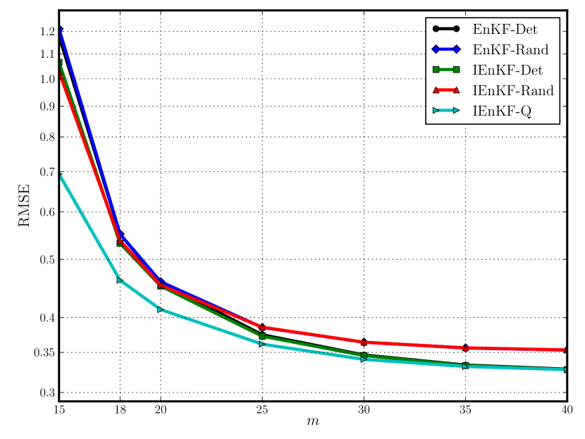
5.1 Test 1: nonlinearity
This test investigates the performance of the schemes depending on the time interval between observations, covering DA regimes from weakly nonlinear to significantly nonlinear. The ensemble size is , chosen so that it is greater than the dimension of the unstable-neutral subspace (which is here and to which we add to account for the redundancy in the anomalies) and hence avoids the need for localisation. Each model variable is observed once at each DA cycle. Model error covariance is set to , where is the time interval between observations in units of the model time-step . For instance, stands for units of the Lorenz-96 model. It is therefore proportional to the cycle length. Since it is added after model integration over the cycle length, the model error variance per unit of time is kept constant. Even though this value of is two orders of magnitude smaller than when , we found it to be realistic. Indeed, the standard deviation of the perturbation added to the truth of the synthetic experiment is in that case, to be compared to a root mean square error of about obtained for the analysis of the EnKF in a perfect model experiment with , the Lorenz-96 model, and the data assimilation setup subsequently described.
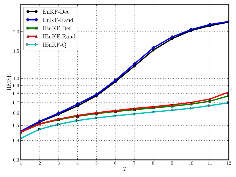
Figure 1 compares the performance of the EnKF, the IEnKF and the IEnKF-Q depending on the time interval (in units of ) between observations. From , the iterative methods noticeably outperform the EnKF due to the increasing nonlinearity. For all , the IEnKF-Q consistently outperforms the IEnKF-Rand and IEnKF-Det. Interestingly, this conclusion holds for the weakly nonlinear case . The reason is that the IEnKF-Q internally uses ensemble of size during the minimisation, while the other methods use only ensembles of size . As will be shown in sections 5.2 and 5.3 (Tests 2 and 3), this advantage decreases with larger ensembles.
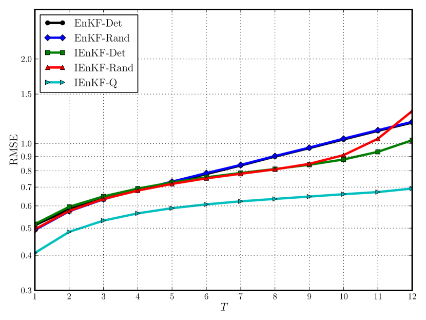
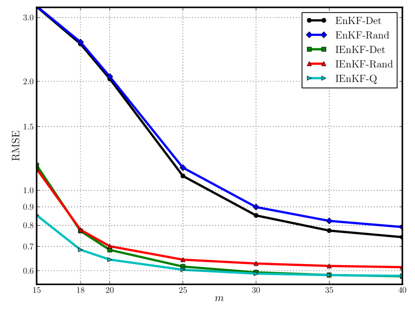
Figure 2 replicates the settings used for Figure 4 of Raanes et al. (2015). Our EnKF-Rand and EnKF-Det schemes correspond to their Add-Q and Sqrt-Core, respectively. Note that Raanes et al. (2015) added model error with covariance after each model step, where is the Kronecker symbol and is the distance on the circle: . Compared to Figure 1, the ensemble size is, accordingly, increased to , and the model error covariance is increased and correlated. It can be seen that the increase in the model error results in a more pronounced advantage of the IEnKF-Q over the other methods. The relative performance of the non-iterative schemes is better than in Figure 1 because of the increased ensemble size.
5.2 Test 2: model noise magnitude
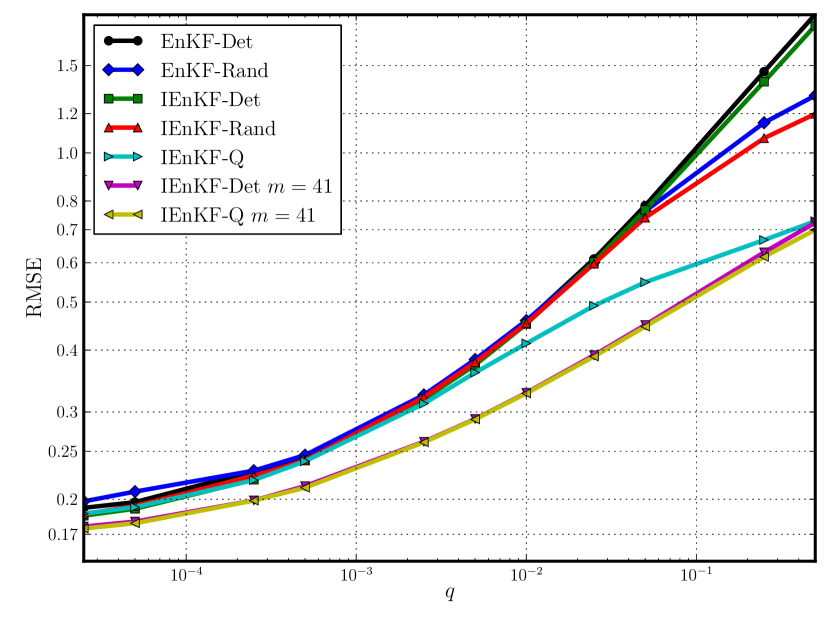
This test investigates the relative performance of the schemes depending on the magnitude of model error both in a weakly nonlinear and significantly nonlinear case. The tests for all schemes involved are conducted with ensemble size . Moreover, results with full-rank ensemble are shown for IEnKF-Det and IEnKF-Q.
Figure 3 shows the performance of the schemes in a weakly nonlinear case . For small model error , all schemes perform similarly; for the IEnKF-Q starts to outperform other schemes; and from the iterative schemes IEnKF-Rand and IEnKF-Det start to outperform their non-iterative counterparts EnKF-Rand and EnKF-Det.
Interestingly, the IEnKF-Q does not show advantage over IEnKF-Det when both use full-rank ensembles (except, perhaps, some very marginal advantage for larger model error ). At a heuristic level, both schemes indeed explore the same model error directions. At a mathematical level, there are indications in favour of this behaviour, including the marginal advantage. Thanks to the decoupling analysis, we see that when the smoothing analysis at of the IEnKF-Q and that of the IEnKF-Det become equivalent. However, the filtering analysis at of the IEnKF-Q, (3), is different albeit close to that of the IEnKF-Det, which is just the forecast of , i.e., the first term of (3). Concerning the update of the anomalies of the ensemble, we have seen that (5) is the of the IEnKF-Det when , and is very close to the expression of for the IEnKF-Q, (5), except maybe when is large.
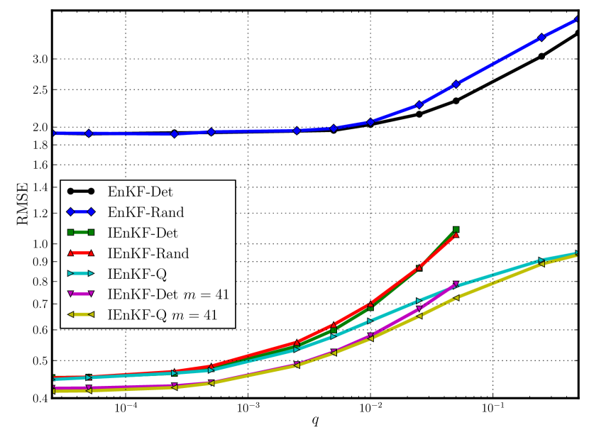
In the significantly nonlinear case (, Figure 4), the non-iterative schemes are no longer able to constrain the model. The empirically modified iterative schemes IEnKF-Rand and IEnKF-Det yield performance similar to the IEnKF-Q up to with the ensemble size , and up to with the ensemble size ; however, apart from underperforming the IEnKF-Q for larger model errors, they also lose stability and are unable to complete cycles necessary for completion of these runs. Interestingly, for very large model error () the IEnKF-Q yields similar performance with the ensemble size of and , with the RMSE much smaller than the average magnitude of the model error . In this regime, the analysis RMSE remains smaller than that obtained with the sole observations (estimated to be by A. Farchi, personal communication). This could be due to the variational analysis which spans the full state space since , and, in this regime, little depends on the prior perturbations .
5.3 Test 3: ensemble size
This test investigates the performance of the methods depending on the ensemble size both in a weakly nonlinear (, Figure 5) and a significantly nonlinear (, Figure 6) case. The model error is set to a moderate magnitude .
In line with the results of Test 2, we observe that the non-iterative schemes do not perform well in the significantly nonlinear case. The IEnKF-Q outperforms the other schemes when using smaller ensembles, but yields a performance similar to that of the IEnKF-Det with a full-rank (or nearly full-rank) ensemble. This is mainly due to its search for the optimal analysis state over a large subspace. Likewise, the performance of the IEnKF-Q degrades when restricting the model error directions to that of the ensemble space (yielding ), and yet remains slightly better than the IEnKF-Det (not shown).
5.4 Test 4: localisation
A couple of numerical experiments are carried out to check that the IEnKF-Q can be made local. However, a detailed discussion of the results is out of scope, since our primary concern is only to confirm the feasibility of a local IEnKF-Q. To this end, we have merged the local analysis as described in Bocquet (2016) and initially meant for the IEnKF in perfect model conditions, with the IEnKF-Q algorithm. The resulting local IEnKF-Q algorithm is given in Appendix A.
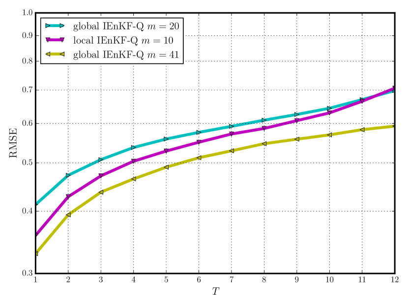
First, we use the same experimental setup as for Figure 1, i.e. the RMSE as a function of . In addition, we consider the local IEnKF-Q with an ensemble size of , which requires the use of localisation. The localisation length is grid points (see Appendix A for its definition). Dynamically covariant localisation is used (see section 4.3 in Bocquet, 2016). The RMSEs are plotted in Figure 7. From Figure 1, we transfer the RMSE curve of the global IEnKF-Q with ensemble size . The same RMSE curve but with was computed and added to the plot. The local IEnKF-Q RMSE curve lies in between those for the global IEnKF-Q with and .
Second, we use the same experimental setup as for Figure 3, i.e. the RMSE as a function of the model error magnitude. From Figure 3, we transfer the RMSE curves of the global IEnKF-Q with ensemble size and . In addition, we consider the local IEnKF-Q with an ensemble size of , which requires the use of localisation. Again, the localisation length is grid points. The RMSEs are plotted in Figure 8. The local IEnKF-Q RMSE curve lies in between those for the global IEnKF-Q with and , with a slight deterioration for very weak model error.
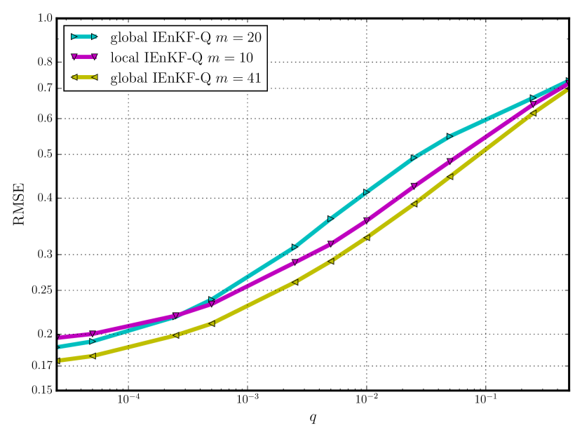
Both tests show that a local IEnKF-Q is not only feasible but also yields very accurate results, with a local -member implementation outperforming a global -member implementation.
6 Discussion
The presence of model error in a DA system causes lossy transmission of information in time. The remote in time observations have less impact on the model state estimates compared to the perfect-model case; and conversely, the current observations have relatively more impact. The latter follows from the KF solution, , which increases the forecast covariance by the model error covariance; therefore the presence of model error shifts the balance between the model state and observations in the analysis towards observations. The former can be seen from the “decoupled” equation (3), when the smoothed state can be obtained essentially in the perfect-model framework using increased observation error according to (30).
This dampened transmission of information shuts down the usual mechanisms of communication in perfect-model linear EnKF systems, such as applying calculated ensemble transforms at a different time or concatenating ensemble observation anomalies within observation window. Because the IEnKF is based on using observations at time for updating the system state at time , it was not intuitively clear whether it could be rigorously extended for the case of imperfect model. Fortunately, the answer to this question has proved to be positive. Moreover, the form of the IEnKF-Q solution (2) suggests that it may be possible to further generalise its framework to assimilate asynchronous observations (i.e, observations collected at different times) within a DA cycle.
In practice, the concept of additive model error is rarely directly applicable, for two reasons. Firstly, the often encountered model errors such as random or some systematic forcing errors, representativeness errors, errors in parametrisations and basic equations and so on are non-additive by nature. Secondly, even if the model error is additive, it is generally difficult to characterise. Because in the KF the model error covariance is directly added to the forecast error covariance, a misspecification of model error will result in a suboptimal, and possibly unbalanced, analysis.
Nevertheless, the additive model error is an important theoretical concept because it permits exact linear recursive solutions known as Kalman filter and Kalman smoother as well as treatment by means of control theory (4D-Var). Furthermore, in 4D-Var the additive model error can be used empirically for regularisation of the minimisation problem that becomes unstable for long assimilation windows (e.g., Blayo et al., 2014, p. 451). Therefore, there may be potential for empirical use of the additive model error in the EnKF to improve numerics. It indeed can often be perfectly feasible to specify some sort of additive model error as a tuneable parameter of a suboptimal system, similarly to the common use of inflation. In fact, a number of studies found that using empirical additive model error in EnKF systems, alone or in combination with inflation, can yield better performance than using inflation only (e.g., Whitaker et al., 2008). Another example of employing model error in a suboptimal system is using (so far without marked success) the hybrid covariance factorised by ensemble anomalies augmenting a small (rank deficient) dynamic ensemble and a large static ensemble (Counillon et al., 2009).
In this study, we have assumed that model error statistics are known. In some simple situations, these could be estimated online with techniques such as those developed by Todling (2015). Nonetheless, using these empirical Bayesian estimation techniques here would have obscured the methodological introduction to the IEnKF-Q.
7 Summary
This study proposes a new method called IEnKF-Q that extends the iterative ensemble Kalman filter (IEnKF) to the case of additive model error. The method consists of a Gauss-Newton minimisation of the nonlinear cost function conducted in ensemble space spanned by the propagated ensemble anomalies and anomalies of the model error ensemble. To simplify the algebraic form of the Gauss-Newton minimisation, the IEnKF-Q concatenates the expansion coefficients and into a single vector , and augments ensemble anomalies and into a single ensemble . After that, the minimisation takes the form (2) similar to that in the perfect-model case.
Algorithmically, the method can take many variations including “transform” and “bundle” versions, and various localisation approaches. An example algorithm suitable for low dimensional systems is presented in section 4. Using this algorithm, the method is tested in section 5 in a number of experiments with the Lorenz-96 model. In all experiments, the IEnKF-Q outperforms both the EnKF and IEnKF adapted for handling model error either in a “stochastic” or “deterministic” way, except in situations with full-rank ensemble and weak to moderate model error, where it performs equally with the IEnKF-Det. Surprisingly, it also outperforms these methods in weakly nonlinear situations, when the solution is essentially found at the very first iteration, and iterative schemes should not have any marked advantage over non-iterative schemes. This is caused by using full-rank (augmented) forecast ensemble anomalies in the analysis, and only reducing the ensemble size back to the initial one at the very end of the cycle. Note that in practice the cost of the IEnKF-Q in high-dimensional systems can be expected to be similar to that of the IEnKF because both methods use ensembles of the same size in propagation.
One interesting feature of the IEnKF-Q is the decoupling of iterations over and made possible in presence of a linear observation operator. In this case, can be found using the (perfect-model) IEnKF with an increased observation error covariance, followed by obtaining in a single iteration. The decoupling can be the underlying reason why in certain situations the IEnKF-Q and IEnKF-Det show equal performance.
The authors would like to thank two anonymous reviewers for their useful comments and suggestions. They are grateful to T. Janjić for her invitation to submit this work. M. Bocquet and J.-M. Haussaire acknowledge the contribution of INSU via the LEFE/MANU DAVE project. CEREA is a member of the Institut Pierre Simon Laplace (IPSL).
Appendix A: Local IEnKF-Q algorithm
Algorithm 2 corresponds to a local analysis variant of the global IEnKF-Q. It stems from merging Algorithm 1 with the local scheme described in Table 2 of Bocquet (2016). The local analyses are looped over the space grid points . Each local analysis uses a local observation error covariance matrix whose inverse has been tapered with the Gaspari-Cohn piecewise rational function (equation (4.10) in Gaspari and Cohn, 1999), where the localisation length is defined to be their parameter.
References
- Bell (1994) Bell BM. 1994. The iterated Kalman smoother as a Gauss-Newton method. SIAM J. Optim. 4: 626–636.
- Bishop et al. (2001) Bishop CH, Etherton BJ, Majumdar SJ. 2001. Adaptive sampling with the ensemble transform Kalman filter. Part I: theoretical aspects. Mon. Wea. Rev. 129: 420–436.
- Blayo et al. (2014) Blayo E, Bocquet M, Cosme E, Cugliandolo LF (eds). 2014. Advanced Data Assimilation for Geosciences. Lecture Notes of the Les Houches School of Physics: Special Issue, June 2012, Oxford University Press: Oxford.
- Bocquet (2016) Bocquet M. 2016. Localization and the iterative ensemble Kalman smoother. Q. J. R. Meteorol. Soc. 142: 1075–1089.
- Bocquet et al. (2010) Bocquet M, Pires CA, Wu L. 2010. Beyond Gaussian statistical modeling in geophysical data assimilation. Mon. Wea. Rev. 138: 2997–3023.
- Bocquet and Sakov (2012) Bocquet M, Sakov P. 2012. Combining inflation-free and iterative ensemble Kalman filters for strongly nonlinear systems. Nonlin. Processes Geophys. 19: 383–399.
- Bocquet and Sakov (2013) Bocquet M, Sakov P. 2013. Joint state and parameter estimation with an iterative ensemble Kalman smoother. Nonlin. Processes Geophys. 20: 803–818.
- Bocquet and Sakov (2014) Bocquet M, Sakov P. 2014. An iterative ensemble Kalman smoother. Q. J. R. Meteorol. Soc. 140: 1521–1535.
- Buizza et al. (1999) Buizza R, Miller M, Palmer TN. 1999. Stochastic representation of model uncertainties in the ECMWF ensemble prediction system. Q. J. R. Meteorol. Soc. 125: 2887–2908.
- Chen and Oliver (2013) Chen Y, Oliver DS. 2013. Levenberg–Marquardt forms of the iterative ensemble smoother for efficient history matching and uncertainty quantification. Comput. Geosci. 17: 689–703.
- Counillon et al. (2009) Counillon F, Sakov P, Bertino L. 2009. Application of a hybrid EnKF-OI to ocean forecasting. Ocean Science 5: 389–401.
- Doucet et al. (2000) Doucet A, Godsill S, Andrieu C. 2000. On sequential Monte Carlo sampling methods for Bayesian filtering. Stat. Comput. 10: 197–208.
- Evensen (1994) Evensen G. 1994. Sequential data assimilation with a nonlinear quasi-geostrophic model using Monte Carlo methods to forecast error statistics. J. Geophys. Res. 99: 10 143–10 162.
- Evensen (2003) Evensen G. 2003. The Ensemble Kalman Filter: theoretical formulation and practical implementation. Ocean Dynam. 53: 343–367.
- Evensen and van Leeuwen (2000) Evensen G, van Leeuwen PJ. 2000. An ensemble Kalman smoother for nonlinear dynamics. Mon. Wea. Rev. 128: 1852–1867.
- Fillion et al. (2017) Fillion A, Bocquet M, Gratton S. 2017. Quasi static ensemble variational data assimilation. Nonlin. Processes Geophys. 0: 0–0. Submitted.
- Gaspari and Cohn (1999) Gaspari G, Cohn SE. 1999. Construction of correlation functions in two and three dimensions. Q. J. R. Meteorol. Soc. 125: 723–757.
- Gu and Oliver (2007) Gu Y, Oliver DS. 2007. An iterative ensemble Kalman filter for multiphase fluid flow data assimilation. SPE Journal 12: 438–446.
- Houtekamer et al. (2009) Houtekamer PL, Mitchell HL, Deng X. 2009. Model error representation in an operational ensemble Kalman filter. Mon. Wea. Rev. 137: 2126–2143.
- Hunt et al. (2004) Hunt BR, Kalnay E, Kostelich EJ, Ott E, Patil DJ, Sauer T, Szunyogh I, Yorke JA, Zimin AV. 2004. Four-dimensional ensemble Kalman filtering. Tellus A 56: 273–277.
- Kalman (1960) Kalman RE. 1960. A new approach to linear filtering and prediction problems. J. Basic. Eng. 82: 35–45.
- Kalnay and Yang (2010) Kalnay E, Yang SC. 2010. Accelerating the spin-up of Ensemble Kalman Filtering. Q. J. R. Meteorol. Soc. 136: 1644–1651.
- Li and Reynolds (2009) Li G, Reynolds AC. 2009. Iterative ensemble Kalman filters for data assimilation. SPE Journal 14: 496–505.
- Lorentzen and Nævdal (2011) Lorentzen RJ, Nævdal G. 2011. An iterative ensemble Kalman filter. IEEE T. Automat. Contr. 56: 1990–1995.
- Lorenz and Emanuel (1998) Lorenz EN, Emanuel KA. 1998. Optimal sites for suplementary weather observations: simulation with a small model. J. Atmos. Sci. 55: 399–414.
- Mandel et al. (2016) Mandel J, Bergou E, Gürol S, Gratton S, Kasanický I. 2016. Hybrid Levenberg-Marquardt and weak-constraint ensemble Kalman smoother method. Nonlin. Processes Geophys. 23: 59–73.
- Raanes et al. (2015) Raanes PN, Carrassi A, Bertino L. 2015. Extending the square root method to account for additive forecast noise in ensemble methods. Mon. Wea. Rev. 143: 3857–3873.
- Rauch et al. (1965) Rauch HE, Striebel CT, Tung F. 1965. Maximum likelihood estimates of linear dynamic systems. AIAA J. 3: 1445–1450.
- Sakov and Bertino (2011) Sakov P, Bertino L. 2011. Relation between two common localisation methods for the EnKF. Comput. Geosci. 15: 225–237.
- Sakov et al. (2010) Sakov P, Evensen G, Bertino L. 2010. Asynchronous data assimilation with the EnKF. Tellus A 62: 24–29.
- Sakov et al. (2012) Sakov P, Oliver DS, Bertino L. 2012. An iterative EnKF for strongly nonlinear systems. Mon. Wea. Rev. 140: 1988–2004.
- Slivinski and Snyder (2016) Slivinski L, Snyder C. 2016. Exploring practical estimates of the ensemble size necessary for particle filters. Mon. Wea. Rev. 144: 861–875.
- Snyder et al. (2015) Snyder C, Bengtsson T, Morzfeld M. 2015. Performance bounds for particle filters using the optimal proposal. Mon. Wea. Rev. 143: 4750–4761.
- Todling (2015) Todling R. 2015. A lag-1 smoother approach to system-error estimation: sequential method. Q. J. R. Meteorol. Soc. 141: 1502–1513.
- Verlaan and Heemink (1997) Verlaan M, Heemink AW. 1997. Tidal flow forecasting using reduced rank square root filters. Stoch. Hydrol. Hydraul. 11: 349–368.
- Whitaker et al. (2008) Whitaker JS, Hamill TM, Wei X, Song Y, Toth Z. 2008. Ensemble data assimilation with the NCEP global forecast system. Mon. Wea. Rev. 136: 463–482.
- Wu et al. (2008) Wu L, Mallet V, Bocquet M, Sportisse B. 2008. A comparison study of data assimilation algorithms for ozone forecasts. J. Geophys. Res. 113: D20 310.
- Yang et al. (2012) Yang SC, Kalnay E, Hunt B. 2012. Handling nonlinearity in the Ensemble Kalman Filter: Experiments with the three-variable Lorenz model. Mon. Wea. Rev. 140: 2628–2646.