Variations on Photon Vacuum Polarization

Abstract

I provide updates for the theoretical predictions of the muon and electron anomalous magnetic moments, for the shift in the fine structure constant $\alpha(M_{Z})$ and for the weak mixing parameter $\sin^{2}\Theta_{W}(M_{Z})$. Phenomenological results for Euclidean time correlators, the key objects in the lattice QCD approach to hadronic vacuum polarization, are briefly considered. Furthermore, I present a list of isospin breaking and electromagnetic corrections for the lepton moments, which may be used to supplement lattice QCD results obtained in the isospin limit and without the e.m. corrections.

 
^∗ Invited talk International Workshop on $e^{+}e^{-}$ collisions from Phi to Psi 2017, 26-29 June 2017, Mainz, Germany

1 Introduction

I present some supplementary material on hadronic vacuum polarization effects which had not been included in my recent book Jegerlehner:2017gek and the Frascati and Capri proceedings Jegerlehner:2017lbd ; Jegerlehner:2015stw . On the data side recent BaBar exclusive channel data, BES-III, KEDR, CMD-3 and SND data are actualized (see these proceedings). Besides continuous progress in $e^{+}e^{-}$ data also lattice QCD (LQCD) is coming closer and actually has provided results not available from elsewhere. This concerns information required for the evaluation of the $\mathit{SU}2$ gauge coupling $\alpha_{2}(s)$ which together with $\alpha(s)$ allows us to calculate the running weak mixing parameter $\sin^{2}\Theta_{W}(s)$. A comparison with lattice results allows one to check the right strategy of the required flavor recombination.

In view of the upcoming new muon $g-2$ experiments LeeRoberts ; Mibe still the biggest challenge are improved $e^{+}e^{-}$ hadronic cross section measurements for improving hadronic vacuum polarization and $\gamma\gamma\to\mathrm{\ hadrons}$ related cross section data for improving the hadronic light-by-light contribution. Substantial progress in lattice QCD calculations of the hadronic current correlators more and more produce important results which complement the dispersive approaches Pauk ; Colangelo .

2 HVP for the muon anomaly

The present status for the hadronic and weak contributions may be summarized by

(6)

For details I refer to Jegerlehner:2017gek ; Jegerlehner:2017lbd ; Jegerlehner:2015stw and references therein (see also Zhang:2015yfi ; Hagiwara:2017zod ). The QED prediction of $a_{\mu}$ is given by (see Aoyama:2012wj ; Laporta:2017okg ; Steinhauser )

$$a_{\mu}^{\rm QED} = \frac{\alpha}{2\pi}+0.765\,857\,423(16)\left(\frac{\alpha}{\pi}\right)^{2}$$ (7)

$$+24.050\,509\,82(28)\left(\frac{\alpha}{\pi}\right)^{3}+130.8734(60)\left(\frac{\alpha}{\pi}\right)^{4}+751.917(932)\left(\frac{\alpha}{\pi}\right)^{5}.$$

Given the CODATA/PDG recommended value of $\alpha$ the theory confronts experiment as collected in Table 1.

Table 1: Standard model theory and experiment comparison

Contribution	Value$\times 10^{10}$		Error$\times 10^{10}$		Reference
QED incl. 4-loops + 5-loops	11 658 471.	886	0.	003	Aoyama:2012wj ; Laporta:2017okg
Hadronic LO vacuum polarization	689.	46	3.	25
Hadronic light–by–light	10.	34	2.	88
Hadronic HO vacuum polarization	-8.	70	0.	06
Weak to 2-loops	15.	36	0.	11	Gnendiger:2013pva
Theory	11 659 178.	3	3.	5	–
Experiment	11 659 209.	1	6.	3	BNL04
The. - Exp. 4.3 standard deviations	-30.	6	7.	2	–

As is well known a “New Physics” interpretation of the persisting 3 to 4 $\sigma$ difference between prediction and experiment requires relatively strongly coupled states in the range below about 250 GeV. Search bounds from LEP, Tevatron and specifically from the LHC already have ruled out a variety of Beyond the Standard Model (BSM) scenarios, so much hat standard motivations of SUSY/GUT extensions seem to fall in disgrace.

There is no doubt that performing doable improvements on both the theory and the experimental side allows one to substantially sharpen (or diminish) the apparent gap between theory and experiment. Yet, even the present situation gives ample reason for speculations. Besides the proton radius puzzle (PRP) Krauth:2017ijq , no other experimental result has as many problems to be understood in terms of SM physics. Note added: The PRP has been solved by now PRP . A new very precise determination of the Rydberg constant in hydrogen spectroscopy reveals a value by 3 $\sigma$’s lower than the 2014 CODATA value.

In any case $a_{\mu}$ constrains BSM scenarios distinctively and at the same time challenges a better understanding of the SM prediction.

3 HVP for the electron anomaly

For the electron anomaly the hadronic and weak contributions read

(13)

The QED prediction of $a_{e}$ including the recent results Aoyama:2012wj ; Laporta:2017okg is given by

$$a_{e}^{\rm QED} = \frac{\alpha}{2\pi}-0.328\,478\,444\,002\,54(33)\left(\frac{\alpha}{\pi}\right)^{2}$$ (14)

$$+1.181\,234\,016\,816(11)\left(\frac{\alpha}{\pi}\right)^{3}-1.91134(182)\left(\frac{\alpha}{\pi}\right)^{4}+7.791(580)\left(\frac{\alpha}{\pi}\right)^{5}.$$

The new quasi–analytic $O(\alpha^{4})$ result by Laporta Laporta:2017okg is certainly a milestone in consolidating the QED part $a_{e}^{\rm QED}$. For extracting $\alpha_{\rm QED}$ the SM prediction

$$a_{e}^{\rm SM}=a_{e}^{\rm QED}+1.723(12)\times 10^{-12}\mbox{(hadronic \& weak)}$$ (15)

is to be confronted with $a_{e}^{\mathrm{exp}}=1159\,652\,180.73(28)$ from experiment aenew as an input. I obtain $\alpha^{-1}(a_{e})=137.035\,999\,1550(331)(0)(27)(14)[333]\;.$ Using $\alpha$ from atomic interferometry, specifically $\alpha(h/M_{\rm Rb11})[0.66\,\mathrm{ppb}]$ [$\alpha^{-1}=137.035999037(91)$], the prediction of $a_{e}$, in units $10^{-12}$, reads $a_{e}^{\mathrm{the}}=1159\,652\,177.28(77)(0)(4)$ [universal] + $2.738(0)$ [$\mu$–loops] + $0.009(0)$ [$\tau$–loops] + $1.693(13)$ [hadronic] + $0.030(0)$ [weak] = $1159\,652\,181.73(77)$ from SM theory, which confronts $a_{e}^{\mathrm{exp}}$. Thus

$$a_{e}^{\mathrm{exp}}-a_{e}^{\mathrm{the}}=-1.00(0.82)\times 10^{-12}\,,$$ (16)

theory and experiment are in excellent agreement. We know that the sensitivity to new physics is reduced by $(m_{\mu}/m_{e})^{2}\cdot\delta a^{\rm exp}_{e}/\delta a^{\rm exp}_{\mu}\simeq 19$ relative to $a_{\mu}$. Nevertheless, one has to keep in mind that $a_{e}$ is suffering less from hadronic uncertainties and thus may provide a safer test. One should also keep in mind that experiments determining $a_{e}$ on the one hand and $a_{\mu}$ on the other hand are very different with different systematics. While $a_{e}$ is determined in a ultra cold environment $a_{\mu}$ has been determined with ultra relativistic (magic $\gamma$) muons so far. Presently, the $a_{e}$ prediction is limited by the, by a factor $\delta\alpha(\mathrm{Rb11})/\delta\alpha(a_{e})\simeq 5.3$ less precise, $\alpha$ available. Combining all uncertainties $a_{\mu}$ is about a factor 43 more sensitive to new physics at present.

4 Hadronic VP and $\alpha(M^{2}_{Z})$

The running electromagnetic fine structure constant is given by $\alpha(s)=\alpha/(1-\Delta\alpha(s))$ with $\Delta\alpha(s)=\Delta\alpha_{\rm lep}(s)+\Delta\alpha^{(5)}_{\rm had}(s)+\Delta\alpha_{\rm top}(s)$ where the non-perturbative part evaluated in terms of $e^{+}e^{-}$ data reads

$$\Delta\alpha_{\rm hadrons}^{(5)}(M_{Z}^{2})=0.027738\pm 0.000158\,[0.027523\pm 0.000119]\,,$$ (17)

where the second result has been obtained with the Euclidean split technique (Adler function approach). The related $\alpha$ then corresponds to

$$\alpha^{-1}(M_{Z}^{2})=128.919\pm 0.022\,[128.958\pm 0.016]\;.$$ (18)

Reducing uncertainties via the Euclidean split technique works as follows: one may split the calculation as

$$\alpha(M_{Z}^{2})=\alpha^{\mathrm{data}}(-s_{0})+\left[\alpha(-M_{Z}^{2})-\alpha(-s_{0})\right]^{\mathrm{pQCD}}+\left[\alpha(M_{Z}^{2})-\alpha(-M_{Z}^{2})\right]^{\mathrm{pQCD}}\,,$$ (19)

where the space-like $-s_{0}$ is chosen such that pQCD is well under control in the deep Euclidean region $-s<-s_{0}$ . The monitor to control the applicability of pQCD is the Adler function $D(Q^{2})$ EJKV98 . It reveals that in the space-like region pQCD works well to predict $D(Q^{2})$ down to $s_{0}=(2.0\,\mbox{GeV})^{2}$. We then may safely use $D^{\mathrm{pQCD}}(Q^{2})$ to calculate perturbatively

$$\alpha(-M_{Z}^{2})-\alpha(-s_{0})=\frac{\alpha}{3\pi}\int\limits_{s_{0}}^{M_{Z}^{2}}\,\rm dQ^{{}^{\prime}2}\frac{D^{\mathrm{pQCD}}(Q^{{}^{\prime}2})}{Q^{{}^{\prime}2}}\;;\;\;D(Q^{2}=-s)=-(12\pi^{2})\,s\,\frac{\rm d\Pi^{\prime}_{\gamma}(s)}{\rm ds}\;.$$ (20)

For the offset $s_{0}=(2.0\,\mbox{GeV})^{2}$ I obtain FJ98 ; Jegerlehner:2008rs $\Delta\alpha^{(5)}_{\rm had}(-s_{0})^{\mathrm{data}}=0.006409\pm 0.000063$, $\Delta\alpha^{(5)}_{\rm had}(-M_{Z}^{2})=0.027483\pm 0.000118$, $\Delta\alpha^{(5)}_{\rm had}(M_{Z}^{2})=0.027523\pm 0.000119$. A shift $+0.000008$ from the 5-loop contribution is included and an error $\pm 0.000100$ has been added in quadrature form the perturbative part. The QCD parameters used are $\alpha_{s}(M_{Z})=0.1189(20)$, $m_{c}(m_{c})=1.286(13)\leavevmode\nobreak\ [M_{c}=1.666(17)]\leavevmode\nobreak\ \mbox{GeV}\,,$ $m_{b}(m_{c})=4.164(25)\leavevmode\nobreak\ [M_{b}=4.800(29)]\leavevmode\nobreak\ \mbox{GeV}\,$, and the evaluation is based on a complete 3–loop massive QCD analysis Chetyrkin:1996cf ; Chetyrkin:1997qi . Note: the Adler function monitored space-like data vs pQCD split approach is only moderately more pQCD-driven than the time-like approach adopted in Davier:2003pw ; Ghozzi:2003yn ; Davier:2009ag ; Zhang:2015yfi and by others. For the first direct measurements of $\Delta\alpha^{(5)}_{\rm had}(s)$ in the $\rho$ resonance region see KLOE-2:2016mgi .

5 Hadronic VP and $\alpha_{2}(M^{2}_{Z})$

In electroweak precision physics non-perturbative hadronic effect primarily show up via the gauge boson self-energy functions. A prominent example is the scale dependence of the weak mixing parameter $\sin^{2}\Theta_{W}(s)$. Note that $\sin^{2}\Theta_{W}(0)/\sin^{2}\Theta_{W}(M_{Z}^{2})=1.02876$ a 3% correction established at $6.5\leavevmode\nobreak\ \sigma$. To understand this one needs precise information of the $\mathit{SU}(2)$ running gauge coupling $\alpha_{2}(s)$. The hadronic shift is related to the correlator $\langle{3\gamma}\rangle$ where “3” marks the 3^rd component of the weak isospin current and “$\gamma$” the e.m. current. As in the case of $\alpha(s)$ the non-perturbative hadronic contribution can be evaluated in terms of $e^{+}e^{-}$ data in conjunction with separating and rewighting the various flavor contributions Jegerlehner:1985gq ; Jegerlehner:2011mw . This has been implemented in the 2016/17 versions of the alphaQED package alphaQED17 . The changes affect the $\alpha_{2}(s)$ routines alpha2SMr17.f, alpha2SMc17.f and the $\sin^{2}\theta_{\rm eff}$ routine ACWMsin2theta.f. The different trials are compared in Tab. 2 and the updated $\sin^{2}\Theta_{W}(s)$ is shown in Fig. 1 for time-like as well as for space-like momentum transfer.

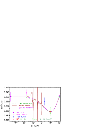
Figure 1: $\sin^{2}\Theta_{W}(Q)$ as a function of $Q$ in the time-like and space-like region. Hadronic uncertainties are included but barely visible in this plot. Uncertainties from the input parameter $\sin^{2}\theta_{W}(0)=0.23822(100)$ or $\sin^{2}\theta_{W}(M_{Z}^{2})=0.23153(16)$ are not shown. Note the substantial difference from applying pQCD with effective quark masses. Future ILC/FCC measurements at 1 TeV would be sensitive to $Z^{\prime}$, $H^{--}$ etc.

Except from the LEP and SLD points (which deviate by 1.8 $\sigma$), all existing measurements are of rather limited accuracy unfortunately! Upcoming experiments will improve results at low space-like $Q$ substantially.

6 Euclidean correlators testing flavor separation and reweighting

Here, we consider the calculation of Euclidean time correlators, which can be calculated in lattice QCD Meyer:2011um ; Bernecker:2011gh . The aim is to compare lattice results with evaluations obtainable from the data. As we know, in the low energy region assuming $\mathit{SU}(3)$ flavor symmetry is not a good approximation. The $\mathit{SU}(2)$ version assuming OZI violating effects to be negligible corresponds to a perturbative reweighting! This has been implemented in the 2012 version of the alphaQED package. Later, lattice evaluations Francis:2013jfa ; Burger:2015lqa revealed this to mismatch the data, while the “old” Jegerlehner:1985gq agreed much better, see Burger:2015lqa . Nevertheless, the $\mathit{SU}(3)$ flavor symmetry argument also looks the be rather crude when looking at correlator in the low energy regime. In place of the untenable assumption that OZI violating terms are small, we may argue by isovector $\rho$ meson dominance (VMD isovector) which suggests an isospin factor 1/2 in place of 9/20 suggested by perturbative reweighting. A 10% difference in the $ud$ part.

Besides the flavor $\mathit{SU}(3)$ inspired weighting

$$\Pi^{3\gamma}_{uds}=\frac{1}{2}\,\Pi^{\gamma\gamma}_{uds}$$

the $\rho$ dominance (exact in the isospin limit) assignment reads

$$\Pi^{3\gamma}_{ud}=\frac{1}{2}\,\Pi^{\gamma\gamma}_{ud}\;;\;\;\Pi^{3\gamma}_{s}=\frac{3}{4}\,\Pi^{\gamma\gamma}_{s}$$

which agrees well with lattice data.

On the $e^{+}e^{-}$ data side, I apply flavor separation by hand, in particular for extracting the isovector part: we skip all final states involving photons like: $\pi^{0}\gamma$, $\eta\gamma$ channels,

as $ud,\;I=0$ we include states with odd number of pions

as $ud,\;I=1$ we include states with even number of pions

as $\bar{s}s$ we count all states with Kaons

States $\eta X$ with $X$ some other hadrons are collected separately, and then split into $q=u,d$ and $s$ components by experimentally established mixing.

Flavor separation is possible only in regions where exclusive channel cross sections are available. We perform this in the region 0.61 GeV to 2.1 GeV. Above this energy only inclusive $R(s)$ measurements are available, and a pQCD reweighting is applied.

Table 2: Variants of flavor recombination of $\langle{3\gamma}\rangle$ in terms of $\langle{\gamma\gamma}\rangle$. LQCD tests strongly disfavor “$\mathit{SU}(2)$” Francis:2013jfa ; Burger:2015lqa

variant		weights			“model”	alphaQED
$\mathit{SU}(3)$	=	$\frac{1}{2}\,[ud]^{I=1}$	+	$\frac{1}{2}[s]$	assuming $\mathit{SU}(3)$ symmetry	hadr5n09
“$\mathit{SU}(2)$”	=	$\frac{9}{20}\,[ud]^{I=1}$	+	$\frac{3}{4}[s]$	perturbative reweighting	hadr5n12	✘
VMD [iso]	=	$\frac{1}{2}\,[ud]^{I=1}$	+	$\frac{3}{4}[s]$	VMD isovector	hadr5n16/17	✔

Key objects in lattice QCD are Euclidean time correlators:

$$I(t)=t^{3}\int_{a}^{\infty}\rm d\,\omega\,\omega^{2}\,\rho(\omega^{2})\,\rm e^{-\omega t}\;;\;\;\rho(s)=\frac{R(s)}{12\pi^{2}}\;.$$ (21)

Normalization (as in  Jegerlehner:1985gq i.e. as weak currents in SM): $D_{\gamma\gamma}(t)=\langle{\gamma\gamma}\rangle(t)\;;\;\;D_{\gamma 3}(t)=\frac{1}{2}\,\langle{\gamma 3}\rangle(t)\;.$ The Euclidean time variable $t$ is in units of 1 fermi fm = 0.1973269631 in GeV^-1, i.e. $t=\mathrm{fm}/E[\mathrm{GeV}]$. For $R(s)=1$ the integral is given by

$$I(t,a,L)[R=1]=\frac{1}{12\pi^{2}}\,t^{3}\int_{a}^{L}\rm d\,\omega\,\omega^{2}\,\rm e^{-\omega t}=\frac{1}{12\pi^{2}}\,\left\{\left(a^{2}t^{2}+2at+2\right)\,\rm e^{-at}-\left(L^{2}t^{2}+2Lt+2\right)\,\rm e^{-Lt}\right\}\;.$$

Calculated in terms of $R(s)$ the flavor-recombination variants listed in Table 2 are compared in Fig. 2 and results for the “best fit” are shown in Fig. 3 for different flavor contents.

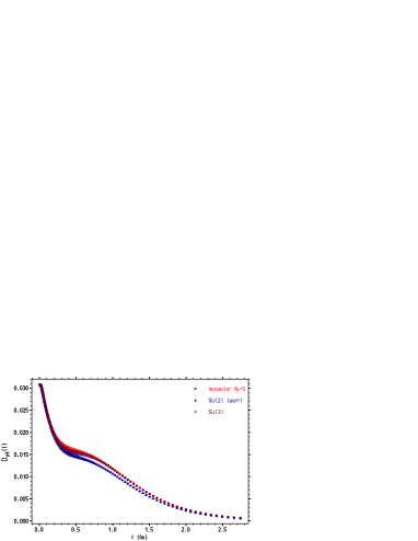
Figure 2: $D_{\gamma 3}(t)$ versions of flavor separation a) VMD isovector, b) in the $\mathit{SU}(2)$ and neglecting OZI suppressed terms = perturbative reweighting, with c) flavor separation in the $\mathit{SU}(3)$ limit including OZI suppressed contributions. Version a) fits best to lattice data, c) shows also reasonable agreement, while b) is significantly off, i.e. perturbative reweighting and/or neglecting OZI suppressed effects is inadequate.

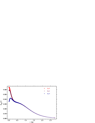
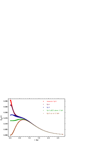
Figure 3: Euclidean correlators. Left: $\langle\gamma\gamma\rangle$ for $N_{f}=3,4$ and $5$ flavors. Right: the same for the $\langle 3\gamma\rangle$ time correlator In the ($u,d$) sector $\langle 3\gamma\rangle$ is $1/2\>\langle\gamma\gamma\rangle$.

7 IB and EM corrections to lattice QCD HVP results

Lattice QCD ab initio calculations of Euclidean current correlators come closer to produce results providing important crosschecks of the standard dispersion relation approach based on $e^{+}e^{-}$ data. Here, in Table 3 I provide and update for $a_{\mu}$, $a_{e}$ and $a_{\tau}$, respectively, isospin breaking (IB) and electromagnetic (EM) corrections not included so far in lattice calculations. A detailed description of the calculations may be found in my book Jegerlehner:2017gek . After submitting the manuscript of the book, I had more time to think carefully about the isospin and e.m. corrections. So I found one of the corrections concerning the dependence on the pion mass not to be the relevant answer to the question what would be the change of a $m_{\pi^{0}}\to m_{\pi^{\pm}}$ shift in lattice results. The shift has been estimated using the Gounaris-Sakurai (GS) parametrization, which however has not the correct dependence on the pion mass, because it includes $M_{\rho}$, $\Gamma_{\rho}$ and $m_{\pi}$ as independent parameters and the shift has been calculated at fixed resonance mass and width. Changing $m_{\pi}$ in the standard Gounaris-Sakurai parametrization (as commonly done in calculating IB effects for the relation between CC (tau) and NC (ee) channels), this is only a partial effect, as the GS formula includes the pion mass dependence in some hidden form. When one uses instead a QFT version as discussed e.g. in Jegerlehner:2011ti (i.e. a QFT provided form of the Breit-Wigner) or also as modeled by he HLS approach one obtains a very different pion mass dependence, as given now in a modified table. The pion mass shift in $|F_{\pi}|^{2}$ is now much larger and compensates largely the large shift in the relation between $R(s)$ and $|F_{\pi}|^{2}$.

So there is an update of Table 5.24 of the book Jegerlehner:2017gek (entries concerning the pion mass dependence) to be replaced by Table 3.

My suspicion that something must be wrong with the GS estimate of the pion mass shift I had when I looked at the shift in the width of the $\rho$ from $m_{\pi}\to m_{\pi^{0}}$, which is actually large (about 2 MeV) but seemed to have a small effect on $|F_{\pi}|^{2}$, which turns out to be an outcome of the GS form.

If one considers the QFT version of the Breit-Wigner, one can see that the cross section $\sigma_{\rm BW}$ at peak

$$\sigma_{\rm BW}=\frac{12\pi}{M_{\rho}^{2}}\,\frac{\Gamma_{ee}}{\Gamma_{\rm tot}}\mathrm{\ \ at\ peak}$$

only depends on the $\rho$ mass and the ratio $\Gamma_{ee}/\Gamma_{\rm tot}$ at $M_{\rho}$, so the dependence on $m_{\pi}$ must be small and results from the fact the the $\pi\pi$ channel is not 100% saturated by the $\rho$ meson. I advocate to perform the $m_{\pi^{0}}\to m_{\pi^{\pm}}$ extrapolation on lattice data directly! Otherwise, utilizing a GS ansatz for the extrapolation of lattice data in the pion mass, requires to take into account the proper pion mass dependence of mass and width of the vector resonance as well.

One is always tempted to take the GS parametrization of the $\pi\pi$ data because experiments as well as the PDG still are extracting the $\rho$ parameters by using the GS formula, which we criticized in Jegerlehner:2011ti . The VMD I ansatz on which GS is based has actually has been criticized by Kroll, Lee and Zumino in 1967 already for lack of e.m. gauge invariance.

Table 3: Neutral channel: muon, electron and $\tau$ missing effects in lattice QCD simulations performed in the isospin limit $m_{d}=m_{u}$ and without QED effects. Effects have been integrated from 300 MeV to 1 GeV

	$\delta a_{\mu}\times 10^{10}$		$\delta a_{e}\times 10^{14}$		$\delta a_{\tau}\times 10^{8}$
Correction type	GS fit	shift	GS fit	shift	GS fit	shift
$I=1$ NC: GS fit of $e^{+}e^{-}$ data [1]	489.21⋆		134.49⋆		167.66⋆
$\omega-\rho$ mixing	491.89	+2.68	135.24	+0.75	168.39	+0.73
FSR of $ee$ $I=1+0$	496.11	+4.22	136.41	+1.17	169.80	+1.41
$\gamma-\rho$ mixing	486.47	-2.74	133.99	-0.50	165.14	-2.52
Elmag. shift $m_{\pi^{0}}\to m_{\pi^{\pm}}$		shift of ⋆
$I=1$ NC $m_{\pi}=m_{\pi^{0}}$ $R(s)$ vs. $|F_{\pi}|^{2}$ [2]	502.01	+12.81	138.21	+3.72	171.22	+3.56
$I=1$ NC $m_{\pi}=m_{\pi^{\pm}}$ $|F_{\pi}|^{2}$ [3]	455.89		125.76		154.23
$I=1$ NC $m_{\pi}=m_{\pi^{0}}$ $|F_{\pi}|^{2}$	441.97	-13.92	121.85	-3.91	150.05	-4.18
Combined $m_{\pi}=m_{\pi^{0}}$	500.91		137.91		170.83
Physical $m_{\pi}=m_{\pi^{\pm}}$ [4]	489.20	1.12	134.49	0.19	167.66	0.62
Elmag. channels HLS12
$\pi^{0}\gamma$	$4.64\pm 0.04$		$1.33\pm 0.04$		$2.11\pm 0.05$
$\eta\gamma$	$0.65\pm 0.01$		$0.17\pm 0.00$		$0.33\pm 0.01$
$\pi^{+}\pi^{-}\pi^{0}$ missing disconnected ?	$5.26\pm 0.15$		$1.76\pm 0.06$		$2.90\pm 0.10$

^[1] $\omega$ switched off,   ^[2] [$|F_{\pi}|^{2}$ fixed],   ^[3] [BW $\rho$ FF],   ^[4] plus e.m. shift in mass&width of the $\rho$

For the charged channel the corresponding results are collected in Table 4.

Table 4: Charged channel: missing effects in lattice QCD simulations performed in the isospin limit $m_{d}=m_{u}$ and without QED effects. Tabulated are the effects $\delta a_{\ell}$ ($\ell=\mu.e,\tau$) integrated from 300 MeV to 1 GeV

	$\delta a_{\mu}\times 10^{10}$		$\delta a_{e}\times 10^{14}$		$\delta a_{\tau}\times 10^{8}$
Correction type	GS fit	shift	GS fit	shift	GS fit	shift
GS fit of $\tau$ data	505.32		139.22		171.35
$+\delta M_{\rho},\,+\delta\Gamma_{\rho}$	501.44	-3.88	138.16	-1.06	170.04	- 1.31
$1/G_{\rm EM}$	504.62	-0.70	138.94	-0.28	171.51	+ 0.16
$\beta_{-}^{3}/\beta_{0}^{3}$	498.73	-6.59	137.30	-1.92	169.53	- 1.82
$I=1$, LQCD type	494.15	-11.17	135.96	-3.26	168.38	- 2.97

Summing up the various corrections yields the results listed in Table 5.

Table 5: Neutral channel: total shifts for $a_{\ell}$ ($\ell=\mu,e,\tau$)

type of correction	$\delta a_{\mu}\times 10^{10}$	$\delta a_{e}\times 10^{12}$	$\delta a_{\tau}\times 10^{8}$
iso+em from $\pi\pi$ channel :	+4.16(4)	+ 1.42(1)	-0.38(0)
incl e.m. decays $\pi^{0}\gamma$ and $\eta\gamma$ :	+ 5.29(4)	+ 1.19(4)	+ 2.06(7)
missing $\phi\to\pi^{+}\pi^{-}\pi^{0}$ ?:	+ 5.26(15)	+ 1.35(4)	+ 2.78(8)
sum	14.71(16)	3.96(6)	4.46(11)

Which of the corrections has to be supplemented depends on the what and whatnot has been included in a given lattice QCD calculation.

Acknowledgments: I thank the organizers of the Phi to Psi 2017 Workshop at Mainz for the kind invitation and the kind hospitality and DESY for the support.

References

- (1) F. Jegerlehner, The Anomalous Magnetic Moment of the Muon, Springer Tracts Mod. Phys. 274, pp.1 (2017), doi:10.1007/978-3-319-63577-4
- (2) F. Jegerlehner, arXiv:1705.00263 [hep-ph].
- (3) F. Jegerlehner, EPJ Web Conf. 118, 01016 (2016)
- (4) B. Lee Roberts, FNAL Experiment, these proceedings
- (5) Tsutomu Mibe, JPARC Experiment, these proceedings
- (6) Gilberto Colangelo, HLBL Dispersive theory Bern, these proceedings
- (7) Vladiszlav Pauk, HLBL Dispersive theory Mainz, these proceedings
- (8) A. Kurz, T. Liu, P. Marquard, M. Steinhauser, Phys. Lett. B 734, 144 (2014)
- (9) Z. Zhang, EPJ Web Conf. 118, 01036 (2016) and these proceedings
- (10) K. Hagiwara et al., Nucl. Part. Phys. Proc. 287-288, 33 (2017); T. Teubner, these proceedings
- (11) T. Aoyama, M. Hayakawa, T. Kinoshita, M. Nio, Phys. Rev. Lett. 109, 111807 (2012); ibid. 111808 (2012); Phys. Rev. D 91, 033006 (2015)
- (12) S. Laporta, Phys. Lett. B 772, 232 (2017)
- (13) A. Kurz et al., PoS LL 2016, 009 (2016); M. Steinhauser, these proceedings
- (14) C. Gnendiger, D. Stöckinger, H. Stöckinger-Kim, Phys. Rev. D 88, 053005 (2013)
- (15) G. W. Bennett et al. [Muon (g-2) Collab.], Phys. Rev. Lett. 92, 161802 (2004)
- (16) J. J. Krauth et al., arXiv:1706.00696 [physics.atom-ph].
- (17) A. Beyer et al., Science, 358:79 (2017), DOI: 10.1126/science.aah6677.
- (18) B. Odom, D. Hanneke, B. D’Urso, G. Gabrielse Phys. Rev. Lett. 97, 030801 (2006)
- (19) S. Eidelman, F. Jegerlehner, A. L. Kataev, O. Veretin, Phys. Lett. B 454, 369 (1999)
- (20) F. Jegerlehner, In: Radiative Corrections, ed J. Solà (World Scientific, Singapore 1999) pp 75–89
- (21) F. Jegerlehner, Nucl. Phys. Proc. Suppl. 181-182, 135 (2008)
- (22) K. G. Chetyrkin, J. H. Kühn, M. Steinhauser, Nucl. Phys. B 482, 213 (1996)
- (23) K. G. Chetyrkin, R. Harlander, J. H. Kühn. M. Steinhauser, Nucl. Phys. B 503, 339 (1997)
- (24) M. Davier, S. Eidelman, A. Höcker, Z. Zhang, Eur. Phys. J. C 31, 503 (2003)
- (25) S. Ghozzi, F. Jegerlehner, Phys. Lett. B 583, 222 (2004)
- (26) M. Davier et al., Eur. Phys. J. C 66, 127 (2010)
-
(27)
A. Anastasi et al. [KLOE-2 Collab.],
Phys. Lett. B 767, 485 (2017);
G. Venanzoni [KLOE-2 Collab.], arXiv:1705.10365 [hep-ex] and these proceedings - (28) F. Jegerlehner, Z. Phys. C 32, 195 (1986)
- (29) F. Jegerlehner, Nuovo Cim. 034C, 31 (2011) [arXiv:1107.4683 [hep-ph]]
- (30) http://www-com.physik.hu-berlin.de/fjeger/alphaQED17.tar.gz
- (31) H. B. Meyer, Phys. Rev. Lett. 107, 072002 (2011)
- (32) D. Bernecker, H. B. Meyer, Eur. Phys. J. A 47, 148 (2011)
- (33) A. Francis, G. von Hippel, H. B. Meyer, F. Jegerlehner, PoS LATTICE 2013, 320 (2013)
- (34) F. Burger, K. Jansen, M. Petschlies, G. Pientka, JHEP 1511, 215 (2015)
- (35) R. R. Akhmetshin et al. [CMD-2 Collaboration], Phys. Lett. B 527, 161 (2002)
- (36) M. Fujikawa et al. [Belle Collaboration], Phys. Rev. D 78, 072006 (2008)
- (37) F. Jegerlehner, R. Szafron, Eur. Phys. J. C 71, 1632 (2011)
- (38) T. Izubuchi, private communication
- (39) M. Benayoun, P. David, L. DelBuono, F. Jegerlehner, Eur. Phys. J. C 72 (2012) 1848