Abstract

An implementation of the Monte Carlo (MC) phase space generators coupled with adaptive MC integration/simulation program FOAM is presented. The first program is a modification of the classic phase space generator GENBOD interfaced with the adaptive sampling integrator/generator FOAM. On top of this tool the algorithm suitable for generation of the phase space for an reaction with two leading particles is presented (double-peripheral process with central production of particles). At the same time it serves as an instructive example of construction of a self-adaptive phase space generator/integrator with a modular structure for specialized particle physics calculations.

1 Introduction

The need for an efficient phase space generation of multiparticle final states resulted in a large number of programs. These tools offers various degree of generality of the application that improve the integration of the differential cross sections. In addition, they allow for efficient generation of events with unit weight. Such feature is needed especially when the very time consuming detector simulation is involved. These programs employ the sampling methods which aim at the minimisation of the integrand variance. One example of efficient strategy is described in [EWas]. The $n$-body phase space parametrised by $3n-4$ independent variables is divided into the manageable subsets (modules) to be handled by techniques which reduce the variance of the result (e.g. importance sampling [PeneKrzywickiCPS] or [Jadach_cylindrical] and the references therein, or the adaptive integration like VEGAS [VEGAS] or FOAM [Jadach-FOAM]). This strategy described in [EWas] was implemented as the parton level Monte Carlo Event Generator AcerMC [PeneKrzywickiCPS] with interfaces to PYTHIA 6.4 [pythia6.4] and other hadronisation programs. Program described in this paper follows in principle the same strategy but its construction assumes the non-perturbative, e.g. Regge, hadron level amplitudes. Moreover, it is designed to efficiently generate the exclusive final states produced in the diffraction processes at very high energy as measured for example at RHIC or at the LHC. As an example the algorithm presented in this paper as GenExLight has been applied to the reaction

$$\begin{array}[]{c}p+p\rightarrow 2p+2\pi^{+}+2\pi^{-},\end{array}$$ (1)

the continuum production of the pion pairs for which one sets restrictive bounds on the transverse momenta of the final state protons – the leading particles. For a thorough physics discussion of the above reaction see [4pi].
The matrix elements for reactions described the Regge model are strongly localised in a small volume of the phase space. Therefore the generation applying the adaptive scanning of the integrand function gives one of the best, most general and flexible approach to solve such problems. To the class of the most general adaptive MC integrators belong VEGAS  [VEGAS] and FOAM  [Jadach-FOAM]. In our toolbox FOAM was selected as it is easily available within the ROOT [ROOT_site] library. However, the generators presented here can be easily adapted to use other MC integrators such as e.g. VEGAS.

The paper is organized as follows. Section 2 presents the augmented algorithm of the phase space generation based on the Raubold-Lynch spherical decay algorithm [James] and interfaced with the external program FOAM for adaptive Monte-Carlo integration. In section 3 a test of the considered tool efficiency is presented. In section 4 an example of the specialized self-adapting phase space generator (employing TDecay as a basic module, which is also described there) is presented. This code designed for the efficient generation of the double-peripheral processes with two leading particles. A test of its efficiency is presented in section LABEL:GenExLight-test. The kinematical formulae derivations and the program technical details are described in the Appendices LABEL:first_appendix, LABEL:second_appendix, LABEL:third_appendix. One should note that the methods presented below are incorporated within the GenEx (the Generator for Exclusive processes) MC code [GenEx]. However, in the present publication, they are described as the stand-alone tools, each with its own area of applications and which can be used to construct minimalistic and case-dedicated MC generators.

2 TDecay – spherical phase space generation algorithm

In this section modifications of the original Raubold-Lynch algorithm [James] implemented in ROOT  [ROOT_site] as the TGenPhaseSpace class will be presented. This modification will be called further TDeacy. The changes allow interfacing the algorithm with external adaptive Monte Carlo simulators e.g FOAM. In addition, instead of the relative weight (i.e. probability of the particular phase space configuration of final particles) we provide absolute phase space weight according to Pilkuhn convention  [Pilkuhn] (compare with [Hagedorn]).

First, let us consider the integral of some function $f(P;p_{1},\ldots,p_{N})$ over the phase space

$$\int dLips(s;p_{1},\ldots,p_{N})f(P;p_{1},\ldots,p_{N}),$$ (2)

where the sum $P$ of the four-momenta of $N$ particles $\{p_{i}\}_{i=1}^{N}$ is conserved, the Lorentz invariant phase space measure is given by

$$dLips(s;p_{1},\ldots,p_{N})=(2\pi)^{4}\delta^{4}\left(P-\sum_{i=1}^{N}p_{i}\right)dLips(p_{1},\ldots,p_{N}),$$ (3)

where $s=P^{2}$ and, finally,

$$dLips(p_{1},\ldots,p_{N})=\prod_{i=1}^{N}\frac{d^{3}p_{i}}{(2\pi)^{3}2E_{i}}.$$ (4)

With substitution

$$f(P;p_{1},\ldots,p_{N})=\frac{|\mathcal{M}|^{2}}{2[\lambda(s,m_{a}^{2},m_{b}^{2})]^{1/2}},$$ (5)

where $\mathcal{M}$ denotes the matrix element for process $p_{a}+p_{b}\rightarrow p_{1}+p_{2}+...+p_{N}$, $P=p_{a}+p_{b}$ and $\lambda(s,m_{a}^{2},m_{b}^{2})=[s-(m_{a}+m_{b})^{2}][s-(m_{a}-m_{b})^{2}]$, the integral (2) represents its cross section $\sigma(s)$. The substitution

$$f(P;p_{1},\ldots,p_{N})=\frac{|\mathcal{M}|^{2}}{2M},$$ (6)

where $M=\sqrt{P^{2}}$ and $\mathcal{M}$ denotes the matrix element for the decay $P\rightarrow p_{1}+p_{2}+...+p_{N}$, the integral in Eq. (2) represents its total width $\Gamma$.

The original Raubold-Lynch idea is sketched in Fig. 1. For a given set of the final particles and the decaying initial state object (marked as a black blob in Fig. 1) of specified four-momentum, one should generate sequential binary decays of intermediate particles until all final state particles are created (see Fig. 1).

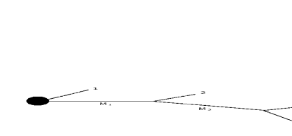
Figure 1: Decay of a central mass object into four final particles. For $n>2$ final state particles there are $n-2$ intermediate particles which masses are ordered $M_{1}>M_{2}>\ldots$.

Each step produces a factor derived from the recurrence relation for phase space  [Pilkuhn]:

$$dLips(s;p_{1},\ldots,p_{m},p_{m+1},\ldots,p_{N})=\\ dLips(s;p_{1},\ldots,p_{m},P_{r})\frac{1}{2\pi}dLips(s_{r};p_{m+1},\ldots,p_{N}),$$ (7)

where the intermediate particle has four-momenta $P_{r}=\sum_{i=m+1}^{N}p_{i}$ and $s_{r}=P_{r}^{2}$. Each of $N-1$ binary decays requires two random variables to generate the angle $\phi$ and $\cos(\theta)$ that fix the direction of the momentum vector of decaying particles. In addition $N-2$ random variables are needed to generate the intermediate masses $M_{1}>M_{2}>\ldots$, which have to be ordered to fulfil the energy conservation constraints. This is achieved using the following formulae:

$$M_{k}=\sum_{i=1}^{k}M_{i}+\left(\sqrt{s}-\sum_{i=1}^{N}M_{i}\right)x_{k};\quad k=2,3,\ldots,N-1$$ (8)

where $0\leq x_{k-1}\leq x_{k}\leq 1$ for k=3,…N-1. Thus TDecay requires on input the set of $2(N-1)+N-2=3N-4$ random numbers (transferred from FOAM) and $N-2$ of them are required to be in the ascending order. The random set which is not properly ordered can be either rejected or sorted in ascending order. In the latter case $(N-2)!$ permutations of the sorted random variables correspond to $(N-2)!$ points of the FOAM probabilistic space which are mapped to single point in the physical phase space. It is therefore like the original FOAM probabilistic space was divided into $(N-2)!$ pieces and every one of them corresponded to the same physical phase space. Therefore, when integrating over such ’multiplied’ FOAM probabilistic space one has to divide the integrand by the factor $(N-2)!$ to avoid multiple counting [PeneKrzywickiCPS]. In the former case, when not properly ordered random sets are rejected, only $1/(N-2)!$ of the whole FOAM probabilistic space is used. Then, the efficiency of the exploration is strongly decreased, especially when the integrand has very small support in the phase space. For this reasons TDecay sorts $n-2$ variables.

The algorithm of TDecay is realized in six steps:

1. Input: rand[$3N-4$] - set of $3N-4$ random numbers; $N$ - the numbers of particles to generate; m[$N$] - array of masses of final particles; $P$ - the decaying particle four-momenta;

2. Check if the decay is energetically allowed: $\sqrt{P^{2}}>\sum_{i=1}^{N}m[i]$;

3. Sort in ascending order the first $N-2$ random numbers; the additional weight factor is $\frac{1}{(N-2)!}$;

4. Generate $N-2$ intermediate masses using sorted random numbers and Eq. (8);

5. For all final particles:

   1. Calculate $|\vec{p}_{i}|$ from the two body decay of the $(i-1)$-th intermediate object to $i$-th particle and $i$-th intermediate object;

   2. Generate $cos(\theta)$ and $\phi$ angle using two random number and rotate $\vec{p}_{i}$ from the OZ axis into a given direction given by these variables;

   3. Perform a Lorentz boost from the centre of mass frame of $i-1$ intermediate object into rest frame of the whole event;

   4. Update the weight for the binary decay;

6. For all final particles perform boost from the centre of mass frame of $P$ to the rest frame;

The above described algorithm represents only a minor modification of the TGenPhaseSpace algorithm from ROOT library. Its implementation requires detailed description which is provided in Appendix LABEL:first_appendix.

3 TDecay – the efficiency test

The program using TDecay was tested for the generation efficiency of the unweighted events (i.e. events with unit weight) measured by the time $t_{gen}$ needed to generate one such event. The performance of TDecay is compared to that of the TGenPhaseSpace, the non-adaptive implementation of the Raubold-Lynch algorithm, using the standard rejection sampling for generation of the unweighted events. Both programs perform their task in two steps. In the case of TGenPhaseSpace the maximal value of the integrand distribution $WtMax$ is searched for in the exploration step, using random sampling points in the whole domain. The next step is the rejection sampling - an event is rejected if its $weight$ fulfils

$$weight<randRej\times maxWt,$$ (9)

where $randRej\in[0;1]$ is the random number generated from the uniform distribution on the unit interval. Otherwise the event is accepted with $weight=1$. The efficiency of the random sampling increases with diminishing weight variance.

In the case of TDecay the FOAM subdivides the domain of the integrand into $ncell$ cells (see Appendix LABEL:first_appendix) in such a way that the weight variance within cell is minimised during the exploration step. The rejection sampling performed cell by cell in the generation step is then more effective and with enough cells it may reach almost $100\%$ efficiency.

When comparing TDecay with TGenPhaseSpace it is important to set the exploration step parameters in such a way that $WtMax$ (global and by cell) is sufficiently well determined. The event generation time, $t_{gen}$, does not include the time needed to perform the exploration step. For the comparative TDecay-TGenPhaseSpace test the number of events generated in the TGenPhaseSpace exploration step was equal to $n_{cell}\times n_{sample}=10^{8}$ where $n_{cell}=10^{4}$ and $n_{sampl}=10^{4}$ are FOAM settings for TDecay run. The number of generated events was set to $10^{5}$ for both programs, $|\mathcal{M}|^{2}=1$, $\sqrt{(}s)=200~{}\rm{GeV}$. Calculation has been performed for 4, 5, and 6 final state particles ($\pi$ mesons). Results are presented in the Tab. 1.

N	$t_{genA}[\rm{ms}]$	$t_{genNA}[\rm{ms}]$	$t_{genNA}/t_{genA}$	$\sigma_{A}$	$\sigma_{NA}$
4	5.3	21.6	0.25	$8.02$	$8.1$
5	5.7	5.5	1.04	$1410$	$1410$
6	4.0	4.0	1.00	$46080$	$46060$

Table 1: Comparison of times of generation of events with unit weight and values of integral using adaptive (A) TDecay program with FOAM setting $n_{cell}=10^{4}$;$n_{sample}=10^{4}$ and non-adaptive (NA) TGenPhaseSpace with $10^{8}$ events in the exploration step. In both cases the matrix element $\mathcal{M}$ is set to 1 and $\sqrt{s}=200~{}\rm{GeV}$. N is the number of generated final state particles,$t_{...}$ with subscripts genA and genNA for adaptive (A) and non-adaptive (NA) sampling is the generation time of single event. The errors for adaptive ($\sigma_{A}$) and non-adaptive ($\sigma_{NA})$ integral (in arbitrary units) are indicated by the last significant digit. Tests were performed on Intel Xeon E5-2680 v3 @ 2.5 GHz.

We can see that for the unit matrix element the adaptive sampling provided by FOAM offers some advantage for N=4 and almost identical generation time, $t_{gen}$, for $N=5,6$ due to insufficient number of cells in the exploration step. The advantage becomes evident when the phase space is restricted by the matrix element or for much larger $n_{cell}\times n_{sampl}$ FOAM setting. This is illustrated in the next comparative test, in which the matrix element represents the Gaussian distribution of particles with the transverse momenta $p_{ti}$ with respect to OZ axis:

$$\mathcal{M}(P;p_{1},p_{2},...p_{N})=\prod_{i=1}^{N}\exp\left(\frac{-p_{ti}^{2}}{2\rho^{2}}\right).$$ (10)

We use the same program settings as above and change both the number of final particles and the departure from spherical symmetry of the matrix element, regulated by the parameter $\rho$. The advantage of the adaptive sampling increases with number of particles and depending on the $\rho$-value the improvement can reach many orders of magnitude in generation time. The results of the test are presented in the Tab. 2. For $N=5,6$ and $\rho\leq 5$ TGenPhaseSpace can not produce $10^{5}$ events within 3 days and calculations were abandoned.

N	$\rho$ [GeV]	$t_{genA}[\rm{ms}]$	$t_{genNA}[\rm{ms}]$	$t_{genA}/t_{genNA}$	$\sigma$ A	$\sigma$ NA
4	5	1.56	1231.3	0.0013	7.25	7.58
4	10	0.75	159.03	0.0047	2.08	2.08
4	15	0.64	74.63	0.0080	7.91	7.91
5	10	4.03	456.5	0.009	1.928	1.93
5	15	2.66	211.54	0.013	1.363	1.35
6	10	7.39	426.25	0.017	1.442	1.44
6	15	4.33	457.30	0.009	1.796	1.79

Table 2: Comparison of the generation times of events having the unit weight and the values of integral obtained using adaptive (A) TDecay program with FOAM settings $n_{cell}=10^{4}$; $n_{sample}=10^{4}$ and non-adaptive (NA) TGenPhaseSpace with $10^{8}$ events in the exploration step. In both cases the matrix element $\mathcal{M}$ is set to the multi-gauss distribution (10), and $\sqrt{s}=200~{}\rm{GeV}$. N is the number of generated final state particles, $t_{...}$ with subscripts genA and genNA for adaptive (A) and non-adaptive (NA) sampling is the generation time of single event. The errors of adaptive ($\sigma_{A}$) and non-adaptive ($\sigma_{NA})$ integral (in arbitrary units) are indicated by the last significant digit. The tests were performed on Intel Xeon E5-2680 v3 @ 2.5 GHz.

4 GenExLight – adaptive phase space integration/generation

In principle TDecay as an adaptive sampling phase space generator/integrator is an universal tool which can deal with any matrix element, provided that FOAM is set up with a sufficient number of cells and samplings per cell. However, in many situations, application of the strategy outlined in [EWas] (see Introduction), which combines the adaptive sampling with the appropriate change of some integration variables, appears to be necessary for practical reasons (computation time). The aim of the variables change is to efficiently generate these events the most restricted either by the matrix element or by the experimental cut. In the following, we describe GenExLight, the phase space generator with a modular structure and the adaptive integrator. It can be treated as a light version of GenEx [GenEx] that can be quickly adapted to specialized particle physics calculations. The code we describe below is adapted for the high energy processes in which the four-momentum transfer to two final state particles, so-called leading particles, is strongly (e.g. exponentially) restricted. The central particle production in the multi-peripheral processes  [LSf0], [LS2pi], [4pi] is an example. This code, without a complicated object oriented structure, allows even beginners to modify it to the particular applications. At the end of this section we provide examples of possible modifications.

The structure of GenExLight is presented in Fig. 2. As a base it uses TDecay class described previously.

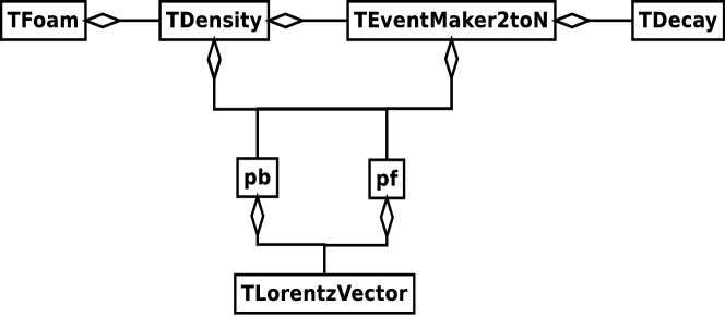
Figure 2: Class diagram of the generator.

The TFoam class of adaptive Monte Carlo simulator requires TDensity class which provides integrand - a function of the four-momenta of the particles that are derived from the random numbers provided by TFoam in TEventMaker2toN. This class generates two leading particles and a central object which then is decayed by TDecay into $N-2$ remaining particles (see Fig. 3). Events are accessible in the tables $pb$ for beam particles and $pf$ for final particles that contains TLorentzVector elements.

Construction of the TEventMaker2toN class uses kinematics derived in [LSf0] for the description of the double peripheral process $pp\rightarrow ppf_{0}$. The cross section formula for the reaction $p_{a}+p_{b}\rightarrow\sum_{i=1}^{N}p_{i}$ is:

$$\sigma=\int(2\pi)^{4}\delta^{(4)}\left(p_{a}+p_{b}-\sum_{i=1}^{N}p_{i}\right)\prod_{i=1}^{N}\frac{d^{3}p_{i}}{(2\pi)^{3}2E_{i}}\frac{|\mathcal{M}|^{2}}{2s};$$ (11)

can be transformed to the form appropriate the factorizable matrix element of the process depicted in Fig. 3, it is

fmftempl1 (50,30) pA,pB pA’,k1,k2,k3,k4,pB’ fermion,lab.side=left, lab=$p_{a}$pA,vA fermion,lab.side=left, lab=$p_{1}$vA,pA’ fermion,lab.side=right, lab=$p_{b}$pB,vB fermion,lab.side=right, lab=$p_{2}$vB,pB’ dbl_wiggly,lab.side=right, lab=$q_{1}$vA,v dbl_wiggly,lab.side=left, lab=$q_{2}$vB,v vA,vB .4wv fermion,lab.side=left, lab=$p_{3}$v,k1 fermion,lab.side=left, lab=$p_{4}$v,k2 fermion,lab.side=left, lab=$p_{...}$v,k3 fermion,lab.side=left, lab=$p_{N}$v,k4

Figure 3: The illustration of the kinematics built by TEvantMaker2toN class adapted to integration/generation of the double peripheral central production processes. The peripherally scattered objects $a$ and $b$ do not enter into the phase space occupied by centrally produced particles $3,4,\ldots,N$.