Accurate, rapid identification of dislocation lines in coherent diffractive imaging via a min-max optimization formulation

Abstract

Defects such as dislocations impact materials properties and their response during external stimuli. Defect engineering has emerged as a possible route to improving the performance of materials over a wide range of applications, including batteries, solar cells, and semiconductors. Imaging these defects in their native operating conditions to establish the structure-function relationship and, ultimately, to improve performance has remained a considerable challenge for both electron-based and x-ray-based imaging techniques. However, the advent of Bragg coherent x-ray diffractive imaging (BCDI) has made possible the 3D imaging of multiple dislocations in nanoparticles ranging in size from 100 nm to1000 nm. While the imaging process succeeds in many cases, nuances in identifying the dislocations has left manual identification as the preferred method. Derivative-based methods are also used, but they can be inaccurate and are computationally inefficient. Here we demonstrate a derivative-free method that is both more accurate and more computationally efficient than either derivative- or human-based methods for identifying 3D dislocation lines in nanocrystal images produced by BCDI. We formulate the problem as a min-max optimization problem and show exceptional accuracy for experimental images. We demonstrate a 260x speedup for a typical experimental dataset with higher accuracy over current methods. We discuss the possibility of using this algorithm as part of a sparsity-based phase retrieval process. We also provide the MATLAB code for use by other researchers.

In materials, crystallographic imperfections such as dislocations often dictate performance and properties. For example, dislocation cores can act as fast diffusion sites Heuser et al. (2014); Purja Pun and Mishin (2009); Xiong et al. (2014); Li et al. (2014), mitigate strain and plasticity during structural phase transformations Ulvestad et al. (2017a); Yau et al. (2017a); Gaucherin et al. (2009), and govern crystal growth Frank (1949); Clark et al. (2015); Walker et al. (2004). Increasingly, Bragg coherent x-ray diffractive imaging (BCDI) is being utilized at synchrotron and x-ray free electron laser Clark et al. (2013); Ulvestad et al. (2017b) sources to address this challenge of understanding and optimizing materials properties via tuning of lattice distortions by nondestructively imaging the 3D lattice distortion field under in situ and operando conditions Robinson and Harder (2009); Cha et al. (2013); Watari et al. (2011); Miao et al. (2015); Hofmann et al. (2017); Newton et al. (2010); Cherukara et al. (2016). The typical resolution of the technique is roughly $10^{-4}$ in strain sensitivity and 10–20 nm spatial resolution at 5–10 minute temporal resolution. Recent studies have revealed the 3D dislocation line dynamics in an individual nanocrystal during reactive processes such as hydrogen uptake Ulvestad et al. (2017a); Yau et al. (2017a), battery charging Ulvestad et al. (2015a), crystal growth and dissolution Liu et al. (2017); Clark et al. (2015), and grain growth in polycrystalline materials Yau et al. (2017b). In all these studies, accurate identification of the dislocation line in the reconstructed image is essential to understanding the underlying physics and the dislocation impact. While these studies have shown great promise, the breadth of 3D BCDI dislocation dynamics measurements and techniques could expand substantially if accurate, robust, and rapid methods existed to determine the 3D dislocation line structure. For example, the datasets generated at diffraction-limited storage rings will likely be too large for existing derivative-based and human-in-the-loop-based methods Dietze and Shpyrko (2015), and the “dislocation basis” could potentially be used as a sparse basis to circumvent constraints in phase retrieval Tripathi et al. (2016). Here we present such a method by reformulating the dislocation core identification problem as a min-max optimization problem that can be solved rapidly.

It is counterintuitive that an imaging experiment with 10–20 nm spatial resolution is sensitive to atomic-scale defects such as dislocations. To understand how this is possible, consider the relationship between the continuum representation of the crystal, $\rho(\mathbf{r})$, and the diffraction intensity, $I(\mathbf{q})$ in the far field under a perfectly coherent illumination and in the kinematical scattering approximation Vartanyants and Robinson (2001); Robinson and Harder (2009); Als-Nielsen and McMorrow (2011):

$$I(\mathbf{q})\approx\left|\mathcal{F}\left(\rho(\mathbf{r})e^{i\mathbf{Q}\cdot\mathbf{u}(\mathbf{r})}\right)\right|^{2}.$$ (1)

Here, $\mathbf{r}$ and $\mathbf{q}$ are the real and reciprocal space coordinates, respectively, $\mathcal{F}$ is the Fourier transform that provides the map between these two spaces, $\mathbf{Q}$ is the measured reciprocal lattice vector (e.g., the 111 Bragg peak for a face-centered cubic crystal lattice), and $\mathbf{u}(\mathbf{r})$ is the vector displacement field that is a continuum description of how the atoms are displaced from their equilibrium positions. If we consider a cubic crystal with a screw dislocation along the $z$ direction, then the displacement field is given by $u_{x}=u_{y}=0$ and

$$u_{z}=\frac{b}{2\pi}\theta,$$ (2)

where $b$ is the Burgers vector and $\theta$ measures the angle around the dislocation core Hull and Bacon (2011). If the Bragg peak (reciprocal lattice vector) measured is the $001$ peak, then $\mathbf{Q}\cdot\mathbf{u}(\mathbf{r})=|Q_{001}|\frac{b}{2\pi}\theta=\frac{2\pi}{a}\frac{b}{2\pi}\theta$. The Burgers vector in this case is equal to the lattice spacing in the $z$ direction, and so $\mathbf{Q}\cdot\mathbf{u}(\mathbf{r})=\theta$. Thus, the signature of a dislocation in the complex image is a point around which the phase varies from $0$ to $2\pi$, or $-\pi$ to $\pi$ depending on the chosen convention. This is the maximum “signal” possible in the image phase and is a direct consequence of dislocations introducing large displacement fields. Note that this argument can be extended to other Bragg peaks that are not parallel to the displacement field induced by the dislocation.

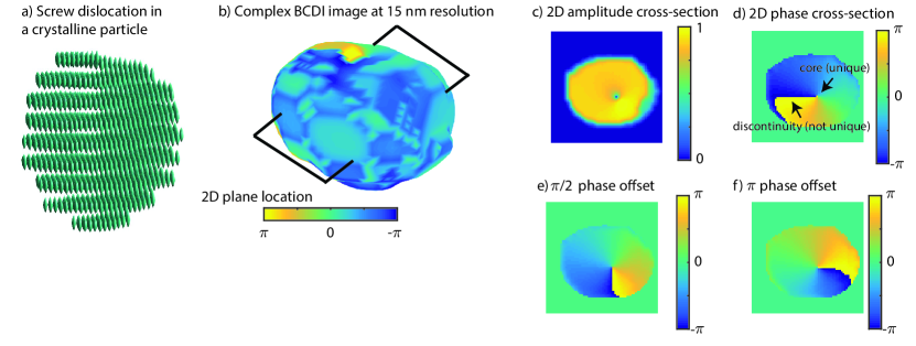
Figure 1: Imaging an atomic-scale defect without atomic resolution. (a) Atoms of a cubic crystal are displaced according to the screw dislocation theoretical displacement field. (b) The $001$ Bragg peak is used after Gaussian blurring to simulate finite resolution and, assuming perfect phase retrieval, to reconstruct a BCDI image of the crystal. The particle shape is represented as an isosurface of the amplitude, which is proportional to the Bragg electron density, while the color projected onto the shape shows the atomic displacement field. (c) The 2D amplitude cross-section corresponding to the location shown in (b). The dislocation core signature can be seen as a low-amplitude region. (d) The 2D phase cross-section; the dislocation manifests itself as a phase vortex, or a region where the phase varies from $-\pi$ to $\pi$. Note that the dislocation core is unique but the phase discontinuity is not. To see why, consider (e) and (f), which have two different global (constant) phase offsets applied; (e) shows a global phase offset of $e^{i\pi/2}$ while (f) shows a global phase offset of $e^{i\pi}$. Both images produce the same diffraction pattern according to Eq. 1. Thus, the reconstructed image is not sensitive to the absolute phase. Different global phase offsets move the phase discontinuity around the dislocation core. This fact is used in the derivative-based dislocation identification method.

To demonstrate a BCDI study of a dislocation, we show in Fig. 1 the atomic and BCDI description of a screw dislocation in a cubic crystal. A periodic array of atoms is created to fill a particular particle shape, and the screw dislocation displacement field is applied (Fig. 1a). The $001$ Bragg peak, blurred by a Gaussian function to simulate a finite resolution, is used to reconstruct the particle image at 15 nm resolution assuming perfect phase retrieval Marchesini (2007); Chapman et al. (2006); Marchesini et al. (2003); Tripathi et al. (2015). The reconstructed BCDI image is complex. The amplitude corresponds to the Bragg, or diffracting, electron density Ulvestad et al. (2015b), while the phase corresponds to the displacement of the atoms from their equilibrium positions. The amplitude is used to draw the isosurface while the phase is projected onto the isosurface as the colormap (Fig. 1b). While the atoms cannot be identified in Fig. 1b because of the finite resolution, there is a key signature in the phase in the form of a phase vortex, or a region where the phase varies from $-\pi$ to $0$ to $\pi$. The 2D cross-sections through the center of the 3D image are shown in Fig. 1c-f. There is a signature of the dislocation core in the amplitude cross-section (Fig. 1c), but this is often difficult to distinguish from the spatial amplitude variation in real experimental data (see, e.g., Fig. 3b). The dislocation signature in the phase is much stronger (Fig. 1d). Again, the reason is that dislocations are large displacements of the atoms from their equilibrium values. However, care must be taken in interpreting the displacement field image. In this case the dislocation core is unique. However, if periodicity is not appropriately accounted for, then the spatial location of the displacement field discontinuity, defined as the jump from $-\pi$ to $\pi$, is not unique, and so this discontinuity cannot be used directly for dislocation identification. To understand why, consider applying a global (constant) phase offset of $e^{i\pi/2}$ to the reconstructed image (Fig. 1e). The diffraction pattern does not change because the factor is a constant and $|e^{i\phi_{0}}|=1$ for all $\phi_{0}$ (see Eq. 1). However, the phase discontinuity line shifts around the dislocation core. An additional example is shown in Fig. 1f for a different phase offset. Thus, the phase discontinuity’s spatial location is not unique, but the dislocation core’s spatial location is unique. All phase offsets shift the discontinuity around the dislocation core, which is exploited in the standard derivative-based method for dislocation core identification described next.

In previous work, dislocation cores were identified by eye or with a derivative-based method that considered a range of phase offsets as shown in Figs. 1d-f. The derivative-based method was previously detailed in Clark et al. (2015); Ulvestad et al. (2017a); only the key steps are repeated here. A derivative of the displacement field is taken in all three orthogonal image directions, thresholding is applied to determine what constitutes a large derivative value, and the locations of these large derivatives are stored. The process is repeated for 360 different global phase offsets in $1^{\circ}$ steps. The intersection (across these 360 offsets) of the locations with large derivatives is used to identify the dislocation core. This process is computationally and memory intensive (three derivatives for each voxel for all 360 phase offsets need to be computed and stored) and requires tuning multiple thresholds. We now define the new algorithm and show how it is both more efficient and more accurate.

Figure 2: Sample phase values from a reconstruction of experimental data (remapped onto a $[0,2\pi]$ scale) for the 25 nearest neighbors of three pixels from distinctly different regions. (a) Sorted values in the neighborhood of a pixel showing minimal phase variation. (b) Sorted values in the neighborhood of a pixel in the dislocation core region. (c) Sorted values in the neighborhood of a pixel in the phase discontinuity region. In our algorithm, the value of $\Psi_{\alpha}$ in (a), (b), and (c) is roughly $0$, $4.2$, and $1.6$, respectively. This suggests a cutoff threshold of 4 for identifying dislocation cores.

We denote by $\hat{x}$ the integer-valued spatial coordinates of a pixel for which we have obtained the complex-valued signal from phase retrieval, where we denote by $\rho(\hat{x})$ and $\theta(\hat{x})$ the amplitude and phase values at that pixel, respectively. We further assume that, in preprocessing, a binary mask has been applied to $\theta$ so that a set of pixels $\hat{x}$ with low amplitude (i.e., $|\rho(\hat{x})|<\tau$ for some specified threshold $\tau>0$) are not considered. We denote the set of all masked pixels $\hat{x}$ by $M$ and its set complement by $\bar{M}$. Such a mask has, for example, been applied to Figs. 3b-c to mask the pixels that have near-zero amplitude. For arbitrary $\hat{x}$ and $\alpha\geq 0$, denote the $\alpha$-neighborhood of $\hat{x}$ by $\mathcal{B}_{\alpha}(\hat{x})=\{\hat{y}:\|\hat{x}-\hat{y}\|_{\infty}\leq\alpha\}$. Consider the $\alpha$-parameterized function of phase offset $\phi_{0}$ and spatial coordinates $\hat{x}$ given by

$$\begin{array}[]{rl}f_{\alpha}(\hat{x},\phi_{0})\triangleq&\displaystyle\max_{\hat{y}\in\mathcal{B}_{\alpha}(\hat{x})\cap\bar{M}}\left[(\theta(\hat{y})+\phi_{0}\right)\equiv 2\pi]\\ -&\displaystyle\min_{\hat{y}\in\mathcal{B}_{\alpha}(\hat{x})\cap\bar{M}}\left[(\theta(\hat{y})+\phi_{0}\right)\equiv 2\pi],\end{array}$$

where we have used $\equiv$ to denote modulo (e.g., $[2\pi+1\equiv 2\pi]=1$). We adopt the convention that if $\mathcal{B}_{\alpha}(\hat{x})\cap\bar{M}=\emptyset$ (i.e., $\mathcal{B}_{\alpha}(\hat{x})\subset M$), then for any value of $\phi_{0}$, $f_{\alpha}(\hat{x},\phi_{0})=0$. Based on our previous discussion, large-magnitude values of the function

$$\Psi_{\alpha}(\hat{x})\triangleq\displaystyle\min_{\phi_{0}\in[0,2\pi)}f_{\alpha}(\hat{x},\phi_{0})$$

signal that $\hat{x}$ is potentially at or near a dislocation core, since $\Psi_{\alpha}(\hat{x})$ represents the least possible length (in radians) of a radius 1 arc containing all the phases, modulo $2\pi$, of pixels in the neighborhood $\mathcal{B}_{\alpha}(\hat{x})$. We are thus interested in solving the min-max problem

$$\max_{\hat{x}}\Psi_{\alpha}(\hat{x})=\max_{\hat{x}}\displaystyle\min_{\phi_{0}\in[0,2\pi)}f_{\alpha}(\hat{x},\phi_{0}).$$ (3)

We note that Eq. 3 is posed as a max-min problem, but we conform with the standard optimization terminology of “min-max” since any max-min problem has an equivalent min-max formulation obtained by negating the objectives. The interpretation of Eq. 3 is that it seeks the largest values of phase differences under the best possible value of the phase offset $\phi_{0}$.

Because $\phi_{0}$ is a continuous parameter and $\hat{x}$ is a discrete pixel location, Eq. 3 is a potentially challenging mixed-integer nonlinear robust optimization problem Belotti et al. (2013). In our case, however, $\Psi_{\alpha}(\hat{x})$ is straightforward to evaluate. We employ the finite list

$$\Theta(\hat{x})\triangleq\left\{[\theta(\hat{y})\equiv 2\pi]:\hat{y}\in\mathcal{B}_{\alpha}(\hat{x})\cap\bar{M}\right\}$$

of the phases associated with all unmasked neighbors of a pixel $\hat{x}$. If $\Theta(\hat{x})$ is empty or composed of a single element, or if $\hat{x}\in M$, then we follow the convention that $\Psi_{\alpha}(\hat{x})=0$. Provided that $\hat{x}$ is not masked and that $\Theta(\hat{x})$ has at least two elements, we run the following procedure.

1. Sort the elements of $\Theta(\hat{x})$ in ascending order, $0\leq\theta_{1}<\dots<\theta_{n}<2\pi$, where $n$ is the number of (distinct) elements in $\Theta(\hat{x})$.

2. Generate a length $n$ array $A$ defined by

   $$\begin{array}[]{rcll}A_{i}&=&2\pi-(\theta_{i+1}-\theta_{i})&i=1,2,\dots,n-1\\ A_{n}&=&\theta_{n}-\theta_{1}.&\\ \end{array}$$

3. Return the least entry of $A$.

In practice, we typically set $\alpha=1$, as in Fig. 2. We remark that in two dimensions, there are at most 9 phases in $\mathcal{B}_{1}(\hat{x})\cap\bar{M}$; in three dimensions, there are at most 27 phases in $\mathcal{B}_{1}(\hat{x})\cap\bar{M}$. Combining this information with the fact that any $\hat{x}\in M$ satisfies $\Psi_{\alpha}(\hat{x})=0$, we can evaluate $\Psi_{\alpha}(\hat{x})$ at every unmasked pixel in a given 2D or 3D dataset in time that is linear in the number of unmasked pixels. The min-max problem in Eq. 3 is then trivially solved by taking the maximum of $\Psi_{\alpha}(\hat{x})$ over all such pixels $\hat{x}$, a task that can be performed in an online fashion (i.e., without explicitly storing the $\Psi_{\alpha}(\hat{x})$ values).

We can gain insight into the algorithm by considering the three cases shown in Fig. 2. Figure 2a shows the sorted experimental phase values in the neighborhood of a pixel in a region of minimal phase variation. The MATLAB range has been shifted from $[-\pi,\pi]$ to $[0,2\pi]$ by applying $+\pi$ to all values. These values were all close to zero in the reconstructed image, and thus they are all close to $\pi$ in the plot. Then, we compute $2\pi$ minus the pairwise differential ($A_{i}$ in step 2). This computation leads to values close to $2\pi$ for most of the pairs, since the differences are near zero. When computing the difference between the last point and the first point, the value is simply the difference, not $2\pi$ minus the difference ($A_{n}$ in step 2). The minimum of this set of values (step 3) is then close to zero, since point 27 and point 1 are close in value. This point is thus not likely to be near a dislocation core.

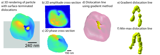
Figure 3: Identifying the dislocation line in images reconstructed from experimental data in which a nanocrystal underwent electrochemical-induced dissolution. (a) The particle shape represented as an isosurface of the amplitude, which is proportional to the Bragg electron density, while the color projected onto the shape shows the atomic displacement field. The same color scale from $-\pi$ to $\pi$ is used as in Fig. 1. (b) The 2D amplitude cross-section corresponding to the central vertical slice. The dislocation core signature can somewhat be seen as a low amplitude region. However, there are two dislocation cores and potentially three low amplitude regions so the identification is ambiguous. (c) The 2D phase cross-section. The two dislocation cores manifest themselves as phase vortices. (d) The 3D dislocation line (yellow) along with the particle shape (semi-transparent red) using the derivative-based method. (e) A close-up view of the dislocation line identified by using the derivative-based method. (f) A close-up view of the line identified using the min-max algorithm. The min-max algorithm is more accurate in identifying the line over all space and more computationally efficient.

Figure 2b shows the sorted experimental phase values in the neighborhood of a pixel in the dislocation core region. Again, we compute $2\pi$ minus the pairwise differential ($A_{i}$ in step 2) and the pairwise differential for point 27 and point 1 ($A_{n}$ in step 2). In this case, the minimum (step 3) in the $2\pi$ minus differential list comes from the difference between point 18 and point 17 (a difference of roughly $2$), and is thus roughly $4.2$. Pixel values above $\pi/2$ indicate potential proximity to a dislocation core, with this likelihood growing as the values approach the $2\pi$ upper bound on $\Psi_{\alpha}$.

Fig. 2c shows the sorted experimental phase values for a pixel outside of, but close to, the phase discontinuity region. In this case, the minimum in the $2\pi$ minus differential list comes from the difference between point 9 and point 10. The differential is approximately $3\pi/2$; since $2\pi-3\pi/2=\pi/2$, the minimum value is approximately $1.62$.

We compare our new method with the derivative-based method for identifying dislocations in images reconstructed from experimental data in Fig. 3. Figure 3a shows the experimental reconstruction of a silver nanoparticle after a dissolution step Liu et al. (2017). The particle shape is represented as an isosurface of the amplitude, which is proportional to the Bragg electron density, while the color projected onto the shape shows the atomic displacement field. The large displacement field on the particle surface is due to the termination of two dislocation lines. A cross section of the amplitude (Fig. 3b) and phase (Fig. 3c) at the particle center show the signature of two dislocation lines. We used the derivative-based method to identify the dislocation line and show the line as a pair of yellow points superimposed onto the particle shape, which is shown as the semi-transparent red isosurface (Fig. 3d). To better visualize the line, we show just the line in Fig. 3e. The line clearly has a horseshoe-like shape, which is indicative of a dislocation transition between edge and screw character Hull and Bacon (2011). The dislocation line shows some artifacts of the derivative-based method, namely, that some parts of the line appear to be larger or smaller than the voxels. Figure 3f shows the line identified with our new algorithm. The line is more clearly identified, and subtle changes in direction are visible. The new algorithm is also 150x faster than the derivative-based method for this 128x128x64 array size (430s versus 3s). The scaling with larger array size is also much better. When tested on a 256x256x96 array with 83,890 nonzero elements, the difference is 1,065s versus 4.7s, a speedup of 260x. This speedup makes incorporating dislocation identification into existing phase retrieval algorithms feasible. It could be used to perform the transformation to the dislocation basis, which tends to be sparse Tripathi et al. (2016). Sparsity using the dislocation basis could be used to circumvent traditional constraints in BCDI, ptychography, and other methods that rely on phase retrieval. One may even be able to use subpixel resolution of angles to further refine dislocation core regions by using more sophisticated min-max algorithms such as that in MMSMW2017.

We developed a new algorithm that is based on minimum differentials in a local neighborhood for identifying dislocation cores in BCDI images. Using experimentally determined images, we demonstrated that this algorithm is both more accurate and computationally efficient. Using the new algorithm, we identified additional geometric features of the dislocation line. The computational speedup opens the possibility of incorporating the dislocation line into the phase retrieval algorithm. For example, the image is sparse in the dislocation basis, and this feature could be exploited to develop new and improved algorithms for phase retrieval and new experimental techniques in which traditional constraints are relaxed. We expect this algorithm will find immediate use in identifying dislocations in reconstructed experimental images, and we provide the algorithm in the supplemental material.

This work, including use of the Advanced Photon Source, was supported by the U.S. Department of Energy, Office of Science, Offices of Basic Energy Sciences (BES) and Advanced Scientific Computing Research (ASCR), under Contract No. DE-AC02-06CH11357. A.U. was supported by the BES Materials Sciences and Engineering Division; M.M. and S.M.W. were supported by the ASCR applied mathematics and SciDAC activities.

References

- Heuser et al. (2014) B. J. Heuser, D. R. Trinkle, N. Jalarvo, J. Serio, E. J. Schiavone, E. Mamontov, and M. Tyagi, Physical Review Letters 113, 1 (2014).
- Purja Pun and Mishin (2009) G. Purja Pun and Y. Mishin, Acta Materialia 57, 5531 (2009).
- Xiong et al. (2014) G. Xiong, J. N. Clark, C. Nicklin, J. Rawle, and I. K. Robinson, Scientific Reports 4, 6765 (2014).
- Li et al. (2014) J. Li, Q. Fang, F. Liu, and Y. Liu, Journal of Power Sources 272, 121 (2014).
- Ulvestad et al. (2017a) A. Ulvestad, M. J. Welland, W. Cha, Y. Liu, J. W. Kim, R. Harder, E. Maxey, J. N. Clark, M. J. Highland, H. You, P. Zapol, S. O. Hruszkewycz, and G. B. Stephenson, Nature Materials 16, 565 (2017a).
- Yau et al. (2017a) A. Yau, R. J. Harder, M. W. Kanan, and A. Ulvestad, ACS Nano 0, null (2017a), pMID: 29035558.
- Gaucherin et al. (2009) G. Gaucherin, F. Hofmann, J. P. Belnoue, and A. M. Korsunsky, Procedia Engineering 1, 241 (2009).
- Frank (1949) F. C. Frank, Discuss. Faraday Soc. 5, 48 (1949).
- Clark et al. (2015) J. N. Clark, J. Ihli, A. S. Schenk, Y.-y. Kim, A. N. Kulak, M. Campbell, G. Nisbit, F. C. Meldrum, and I. K. Robinson, Nature Materials 14, 780 (2015).
- Walker et al. (2004) A. M. Walker, B. Slater, J. D. Gale, and K. Wright, Nature Materials 3, 715 (2004).
- Clark et al. (2013) J. N. Clark, L. Beitra, G. Xiong, a. Higginbotham, D. M. Fritz, H. T. Lemke, D. Zhu, M. Chollet, G. J. Williams, M. Messerschmidt, B. Abbey, R. J. Harder, a. M. Korsunsky, J. S. Wark, and I. K. Robinson, Science (New York, N.Y.) 341, 56 (2013).
- Ulvestad et al. (2017b) A. Ulvestad, M. J. Cherukara, R. Harder, W. Cha, I. K. Robinson, S. Soog, S. Nelson, D. Zhu, G. B. Stephenson, O. Heinonen, and A. Jokisaari, Scientific Reports 7, 9823 (2017b).
- Robinson and Harder (2009) I. Robinson and R. Harder, Nature Materials 8, 291 (2009).
- Cha et al. (2013) W. Cha, N. C. Jeong, S. Song, H.-j. Park, T. C. Thanh Pham, R. Harder, B. Lim, G. Xiong, D. Ahn, I. McNulty, J. Kim, K. B. Yoon, I. K. Robinson, and H. Kim, Nature Materials 12, 729 (2013).
- Watari et al. (2011) M. Watari, R. a. McKendry, M. Vögtli, G. Aeppli, Y.-A. Soh, X. Shi, G. Xiong, X. Huang, R. Harder, and I. K. Robinson, Nature Materials 10, 862 (2011).
- Miao et al. (2015) J. Miao, T. Ishikawa, I. K. Robinson, and M. M. Murnane, Science 348, 530 (2015).
- Hofmann et al. (2017) F. Hofmann, E. Tarleton, R. J. Harder, N. W. Phillips, P.-W. Ma, J. N. Clark, I. K. Robinson, B. Abbey, W. Liu, and C. E. Beck, Scientific Reports 7, 45993 (2017).
- Newton et al. (2010) M. C. Newton, S. J. Leake, R. Harder, and I. K. Robinson, Nature Materials 9, 120 (2010).
- Cherukara et al. (2016) M. J. Cherukara, K. Sasikumar, W. Cha, B. Narayanan, S. Leake, E. Dufresne, T. Peterka, I. McNulty, H. Wen, S. K. Sankaranarayanan, and R. Harder, Nano Letters 17, 1102 (2016).
- Ulvestad et al. (2015a) A. Ulvestad, A. Singer, J. N. Clark, H. M. Cho, J. W. Kim, R. Harder, J. Maser, Y. S. Meng, and O. G. Shpyrko, Science (New York, N.Y.) 348, 1344 (2015a).
- Liu et al. (2017) Y. Liu, P. P. Lopes, W. Cha, R. Harder, J. Maser, E. Maxey, M. J. Highland, N. M. Markovic, S. O. Hruszkewycz, G. B. Stephenson, H. You, and A. Ulvestad, Nano Letters 17, 1595 (2017).
- Yau et al. (2017b) A. Yau, W. Cha, M. W. Kanan, G. B. Stephenson, and A. Ulvestad, Science 356, 739 (2017b).
- Dietze and Shpyrko (2015) S. H. Dietze and O. G. Shpyrko, Journal of Synchrotron Radiation 22, 1498 (2015).
- Tripathi et al. (2016) A. Tripathi, I. McNulty, T. Munson, and S. M. Wild, Optics Express 24, 24719 (2016).
- Vartanyants and Robinson (2001) I. A. Vartanyants and I. K. Robinson, Journal of Physics: Condensed Matter 13, 10593 (2001).
- Als-Nielsen and McMorrow (2011) J. Als-Nielsen and D. McMorrow, Elements of Modern X-Ray Physics (John Wiley & Sons, Inc., 2011).
- Hull and Bacon (2011) D. Hull and D. Bacon, Introduction to Dislocations, 5th ed. (Butterworth-Heinemann, 2011).
- Marchesini (2007) S. Marchesini, Review of Scientific Instruments 78, 011301 (2007), arXiv:0603201 [physics] .
- Chapman et al. (2006) H. Chapman, A. Barty, and S. Marchesini, JOSA A 23 (2006).
- Marchesini et al. (2003) S. Marchesini, H. He, and H. Chapman, Physical Review B 68, 140101 (2003), arXiv:0306174v2 [arXiv:physics] .
- Tripathi et al. (2015) A. Tripathi, S. Leyffer, T. Munson, and S. M. Wild, Procedia Computer Science 51, 815 (2015).
- Ulvestad et al. (2015b) A. Ulvestad, J. N. Clark, R. Harder, I. K. Robinson, and O. G. Shpyrko, Nano Letters 15, 40664070 (2015b).
- Belotti et al. (2013) P. Belotti, C. Kirches, S. Leyffer, J. Linderoth, J. Luedtke, and A. Mahajan, Acta Numerica 22, 1 (2013).