Two Birds with One Stone: Transforming and Generating Facial Images with Iterative GAN

Abstract

Generating high fidelity identity-preserving faces with different facial attributes has a wide range of applications. Although a number of generative models have been developed to tackle this problem, there is still much room for further improvement. In paticular, the current solutions usually ignore the perceptual information of images, which we argue that it benefits the output of a high-quality image while preserving the identity information, especially in facial attributes learning area. To this end, we propose to train GAN iteratively via regularizing the min-max process with an integrated loss, which includes not only the per-pixel loss but also the perceptual loss. In contrast to the existing methods only deal with either image generation or transformation, our proposed iterative architecture can achieve both of them. Experiments on the multi-label facial dataset CelebA demonstrate that the proposed model has excellent performance on recognizing multiple attributes, generating a high-quality image, and transforming image with controllable attributes.

1 Introduction

Image generation gregor2015draw ; Wang2017Tag ; Odena2017Conditional and image transformation Isola2016Image ; zhu2016generative ; yoo2016pixel-level ; Zhu2017Unpaired are two important topics in computer vision. A popular way of image generation is to learn a complex function that maps a latent vector onto a generated realistic image. By contrast, image transformation refers to translating a given image into a new image with modifications on desired attributes or style. Both of them have wide applications in practice. For example, facial composite, which is a graphical reconstruction of an eyewitness’s memory of a face mcquistonsurrett2006use , can assist police to identify a suspect. In most situations, police need to search a suspect with only one picture of the front view. To improve the success rate, it is very necessary to generate more pictures of the target person with different poses or expressions. Therefore, face generation and transformation have been extensively studied.

Benefiting from the successes of the deep learning, image generation and transformation have seen significant advances in recent years dong2014learning ; denoord2016conditional . With deep architectures, image generation or transformation can be modeled in more flexible ways than traditional approaches. For example, the conditional PixelCNN denoord2016conditional was developed to generate an image based on the PixelCNN. The generation process of this model can be conditioned on visible tags or latent codes from other networks. However, the quality of generated images and convergence speed need improvement. In gregor2015draw and yan2015attribute2image , the Variational Auto-encoders (VAE) kingma2014auto-encoding was proposed to generate natural images. Recently, Generative adversarial networks (GAN) goodfellow2014generative has been utilized to generate natural images denton2015deep or transform images zhu2016generative ; Zhu2017Unpaired ; zhang2017age ; ShuYHSSS17 with conditional settings Mirza2014Conditional .

The existing approaches can be applied to face generation or face transformation respectively, however, there are several disadvantages of doing so. First, face generation and face transformation are closely connected with a joint distribution of facial attributes while the current models are usually proposed to achieve them separately (face generation yan2015attribute2image ; li2017generate or transformation zhang2017age ; ShuYHSSS17 ), which may limit the prediction performance. Second, learning facial attributes has been ignored by existing methods of face generation and transformation, which might deteriorate the quality of facial images. Third, most of the existing conditional deep models did not consider to preserve the facial identity during the face transformation  Isola2016Image or generation yan2015attribute2image ;

To this end, we propose an iterative GAN with an auxiliary classifier in this paper, which can not only generate high fidelity face images with controlled input attributes, but also integrate face generation and transformation by learning a joint distribution of facial attributes. We argue that the strong coupling between face generation and transformation should benefit each other. And the iterative GAN can learn and even manipulate multiple facial attributes, which not only help to improve the image quality but also satisfy the practical need of editing facial attributes at the same time. In addition, in order to preserve the facial identity, we regularize the iterative GAN by the perceptual loss in addition to the pixel loss. A quantity metric was proposed to measure the face identity in this paper.

To train the proposed model, we adopt a two-stage approach as shown in Figure 2. In the first stage, we train a discriminator $\mathbf{D}$, a generator $\mathbf{G}$, and a classifier $\mathbf{C}$ by minimizing adversarial losses goodfellow2014generative and the label losses as in Odena2017Conditional . In the second stage, $\mathbf{G}$ and $\mathbf{D}/\mathbf{C}$ are iteratively trained with an integrated loss function, which includes a perceptual component johnson2016perceptual between $\mathbf{D}$’s hidden layers in stage 1 and stage 2, a latent code loss between the input noise $\mathbf{z}$ and the output noise $\tilde{\mathbf{z}}$, and a pixel loss between the input real facial images and their corresponding rebuilt version.

In the proposed model, the generator $\mathbf{G}$ not only generates a high-quality facial image according to the input attribute (single or multiple) but also translates an input facial image with desired attribute modifications. The fidelity of output images can be highly preserved due to the iterative optimization of the proposed integrated loss. To evaluate our model, we design experiments from three perspectives, including the necessity of the integrated loss, the quality of generated natural face images with specified attributes, and the performance of face generation. Experiments on the benchmark CelebA dataset liu2015faceattributes have indicated the promising performance of the proposed model in face generation and face transformation.

2 Related Work

2.1 Facial attributes recognition

Object Recognition method has been researched for a long while as an active topic Farhadi2009Describing ; branson2010visual ; nilsback2008automated especially for human recognition, which takes attributes of a face as the major reference  kumar2009attribute ; cherniavsky2010semi-supervised . Such attributes include but not limited to natural looks like Arched_Eyebrows, Big_Lips, Double_Chin, Male, etc. Besides, some ‘artificial ?attributes also contribute to this identification job, like Glasses, Heavy_Makeup, Wave_Hair. Even some expression like Smiling, Angry, Sad can be labeled as a kind of facial attributes to improve identification. For example, Devi et al. analyze the complex relationship among these multitudinous attributes to categorize a new image parikh2011relative . The early works on automatic expression recognition can be traced back to the early nineties bettadapura2012face . Most of them kumar2009attribute ; berg2013poof: ; bourdev2011describing tried to verify the facial attributes based on the methods of HOG dalal2005histograms and SVM cortes1995support-vector . Recently, the development of the deep learning flourished the expression recognition zhang2014panda: and made a success of performing face attributes classification based on CNN (the Convolutional Neural Networks) liu2015faceattributes . The authors of  liu2015faceattributes even devised a dataset celebA that includes more than 200k face images (each with 40 attributes labels) to train a large deep neural network. celebA is widely used in facial attributes researches. In this paper, we test iterative GAN with it. FaceNet schroff2015facenet: is another very important work on face attributes recognition that proposed by Google recently. They map the face images to a Euclidean space, thus the distance between any two images that calculated in the new coordinate system shows how similar they are. The training process is based on the simple heuristic knowledge that face images from the same person are closer to each other than faces from different persons. The FaceNet system provides a compare function to measure the similarity between a pair of images. We prefer to utilize this function to measure the facial identity-preserving in quantity.

2.2 Conditioned Image Generation

Image generation is an very popular and classic topic in computer vision. The vision community has already taken significant steps on the image generation especially with the development of deep learning.

The conditional models Mirza2014Conditional ; Kingma2014Semi ; denoord2016conditional enable easier controlling of the image generation process. In denoord2016conditional , the authors presented an image generation model based on PixelCNN under conditional control. However, it is still not satisfying on image quality and efficiency of convergence. In the last three years, generating images with Variational Auto-encoders (VAE) kingma2014auto-encoding and GAN goodfellow2014generative have been investigated. A recurrent VAE was proposed in gregor2015draw to model every stage of picture generation. Yan et al. yan2015attribute2image used two attributes conditioned VAEs to capture foreground and background of a facial image, respectively. In addition, the sequential model gregor2015draw ; denton2015deep has attracted lots of attention recently. The recurrent VAE  gregor2015draw mimic the process of human drawing but it can only be applied to low-resolution images; in denton2015deep , a cascade Laplacian pyramid model was proposed to generate an image from low resolution to a final full resolution gradually.

GAN goodfellow2014generative has been applied to lots of works of image generation with conditional setting since Mirza and Osindero Mirza2014Conditional and Gauthier gauthier14 . In denton2015deep , a Laplacian pyramid framework was adopted to generate a natural image with each level of the pyramid trained with GAN. In wang2016generative , the S²GAN was proposed to divide the image generation process into structure and style generation steps corresponding to two dependent GAN. The Auxiliary classifier GAN (ACGAN) in Odena2017Conditional tries to regularize traditional conditional GAN with label consistency. To be more easy to control the conditional tag, the ACGAN extended the original conditional GAN with an auxiliary classifier $\mathbf{C}$.

2.3 Image Transformation

Image transformation is a well-established area in computer vision which could be concluded as “where a system receives some input image and transforms it into an output image johnson2016perceptual ”. According to this generalized concept, a large amount of image processing tasks belong to this area such as images denoise xie2012image , generate images from blueprint or outline sketch Isola2016Image , alternate a common picture to an artwork maybe with the style of Vincent van Gogh or Claude Monet Zhu2017Unpaired ; gatys2015a , image inpainting xie2012image , the last but not the least, change the appointed facial attributes of a person in the image.

Most works of image transformation are based on pixel-to-pixel loss. Like us,  gatys2015a transforms images from one style to another with an integrated loss (feature loss and style reconstruction loss) through CNN. Though the result is inspiring, this model is very cost on extracting features on pre-trained model. Recently, with the rapid progress of generative adversarial nets, the quality of output transformed images get better. The existing models of image transforming based on GAN fall into two groups. Manipulating images over the natural image manifold with conditional GAN belongs to the first category. In zhu2016generative , the authors defined user-controlled operations to allow visual image editing. The source image is arbitrary, especially could lie on a low-dimensional manifold of image attributes, such as the color or shape. In a similar way, Zhang et al. zhang2017age assume that the age attribute of face images lies on a high-dimensional manifold. By stepping along the manifold, this model can obtain face images with different age attributes from youth to old. The remaining works consist of the second group. In Isola2016Image , the transformation model was built on the conditional setting by regularizing the traditional conditional GAN Mirza2014Conditional model with an image mapping loss. Some work considers deploying GAN models for each of the related image domains (.e.g. input domain and output domain), more than one set of adversarial nets then cooperate and restrict with each other to generate high-quality results yoo2016pixel-level ; Zhu2017Unpaired . In yoo2016pixel-level , a set of aligned image pairs are required to transfer the source image of a dressed person to product photo model. In contrast, the cycle GAN Zhu2017Unpaired can learn to translate an image from a source domain to a target domain in the absence of paired samples. This is a very meaningful advance because the paired training data will not be available in many scenarios.

2.4 Perceptual Losses

\begin{overpic}[scale={0.6}]{perceptual_loss.pdf} \par\put(44.0,39.5){{\footnotesize$\mathbf{h}^{0}$}} \put(53.5,39.5){{\footnotesize$\mathbf{h}^{1}$}} \put(63.5,39.5){{\footnotesize$\mathbf{h}^{2}$}} \put(81.0,39.5){{\footnotesize$\mathbf{h}^{i}$}} \par\put(39.0,9.0){{\footnotesize$\mathbf{h}{{}^{0}}_{\text{rebuilt}}$}} \put(48.5,9.0){{\footnotesize$\mathbf{h}{{}^{1}}_{\text{rebuilt}}$}} \put(59.0,9.0){{\footnotesize$\mathbf{h}{{}^{2}}_{\text{rebuilt}}$}} \put(77.0,9.0){{\footnotesize$\mathbf{h}{{}^{i}}_{\text{rebuilt}}$}} \par\end{overpic}

Figure 1: Demonstration of how to train an image transformation model johnson2016perceptual with the perceptual loss. A pretrained network (right yellow part) plays a role in extracting feature information of both ground-truth and rebuilt image through several convolutional layers. For each layer, the semantic differences $L_{i}$ between the two images is calculated. Finally, by reducing the total differences collected through all layers, the image transform model (left part in dashed box) is optimized to rebuild the ground-truth image.

A traditional way to minimize the inconsistency between two images is optimizing the pixel-wise loss tatarchenko2016multi-view ; Isola2016Image ; zhang2016colorful . However, the pixel-wise loss is inadequate for measuring the variations of images, since the difference computed in pixel element space is not able to reflect the otherness in visual perspective. We could easily and elaborately produce two images which are absolutely different observed in human eyes but with minimal pixel-wise loss and vice verse. Moreover, using single pixel-wise loss often tend to generate blurrier results with the ignorance of visual perception information Isola2016Image ; Larsen2015Autoencoding . In contrast, the perceptual loss explores the discrepancy between high-dimensional representations of images extracted from a well-trained CNN (for example VGG-16 simonyan2015very ) can overcome this problem. By narrowing the discrepancy between ground-truth image and output image from a high-feature-level perspective, the main visual information is well-reserved after the transformation. Recently, the perceptual loss has attracted much attention in image transformation area  johnson2016perceptual ; gatys2015a ; Wang2017Perceptual ; dosovitskiy2016generating . By employing the perceptual information, gatys2015a perfectly created the artistic images of high perceptual quality that approaching the capabilities of human; ledig2016photo-realistic highlighted the applying of perceptual loss to generate super-resolution images with GAN, the result is amazing and state-of-art; Wang2017Perceptual proposed a generalized model called perceptual adversarial networks (PAN) which could transform images from sketch to colored, semantic labels to ground-truth, rainy day to de-rainy day etc. Zhu et al. zhu2016generative focused on designing a user-controlled or visual way of image manipulation utilize the perceptual similarity between images that defined over a low dimensional manifold to visually edit images.

A convenient way of calculating the perceptual loss between a ground-truth face $\mathbf{x}_{\text{ground-truth}}$ and a transformed face $\mathbf{x}_{\text{rebuilt}}$ is to input them to a Convolutional Neural Networks (such as the VGG-16 simonyan2015very or the GoogLeNet szegedy2015going ) then sum the differences of their representations from each hidden layers johnson2016perceptual of the network. As shown in Fig. 1 johnson2016perceptual , both of the $\mathbf{x}_{\text{ground-truth}}$ and $vx_{\text{rebuilt}}$ was passed to the pretrained network as inputs. The differences between their corresponding latent feature matrices $\mathbf{h}^{i}$ and $\mathbf{h}^{i}_{\text{rebuilt}}$ can be calculated ($L_{i}=\|\mathbf{h}_{\text{rebuilt}}^{i}-\mathbf{h}^{i}\|$).

The final perceptual loss can be represented as follows,

$$L_{per}=\mathbb{E}_{\{\mathbf{h}_{\text{rebuilt}}^{i},\mathbf{h}^{i}\}}[\sum_{i=1}\alpha_{i}\|\mathbf{h}_{\text{rebuilt}}^{i}-\mathbf{h}^{i}\|]$$

Where $\mathbf{h}_{\text{rebuilt}}^{i},\mathbf{h}^{i}$ are the feature matrices output from each convolutional layers, $\alpha_{i}$ are the parameters to balance the affections from each layers.

For facial image transformation, perceptual information shows its superiority in preserving the facial identity. To take advantages of this property of the perceptual loss, in our proposed model, we leverage it to keep the consistency of personal identity between two face images. In particular, we choose to replace the popular pretrained Network with the discriminator network to decrease the complexity. We will discuss this issue in detail later.

3 Proposed Model

We first describe the proposed model with the integrated loss, then explain each component of the integrated loss.

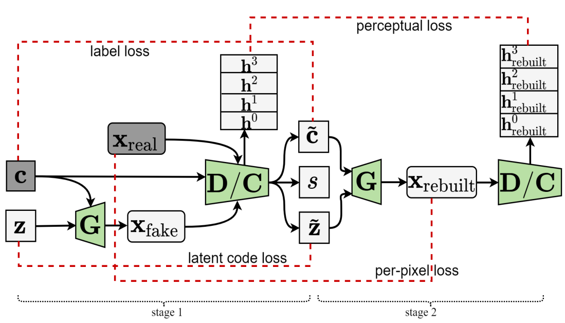
Figure 2: The architecture of our proposed model. Training: the model begin with a original GAN process, the generator $\mathbf{G}$ takes a random noise vector $\mathbf{z}$ and label $\mathbf{c}$ as inputs. It outputs a generated face image $\mathbf{x}_{\text{fake}}$. The discriminator $\mathbf{D}$ receives both $\mathbf{x}_{\text{fake}}$ and a real image $\mathbf{x}_{\text{real}}$, and outputs the probability distribution over possible image sources. An auxiliary classifier $\mathbf{C}$, which shares layers (without the last layer) with $\mathbf{D}$, predicts a label $\tilde{\mathbf{c}}$ and outputs reconstructed noise code $\tilde{\mathbf{z}}$. Meanwhile, $\mathbf{D}$ outputs $s$ (indicates whether the image is fake or real). At the second stage, $\mathbf{G}$ rebuilds the $\mathbf{x}_{\text{real}}$ by generating a $\mathbf{x}_{\text{rebuilt}}$ with $\tilde{\mathbf{z}}$ and $\tilde{\mathbf{c}}$. Then $\mathbf{D}$ iteratively receives $\mathbf{x}_{\text{rebuilt}}$ and updates the hidden layers (from $\mathbf{h}$ to $\mathbf{h}_{\text{rebuilt}}$). During testing, we can deal with both face generation and transformation. By sampling a random vector $\mathbf{z}$ and a desired facial attribute description, a new face can be generated by $\mathbf{G}$. For face transformation, we feed the discriminator $\mathbf{D}$ a real image $\mathbf{x}_{\text{real}}$ together with its attribute labels $\mathbf{c}$, then we get a noise representation $\tilde{\mathbf{z}}$ and label vector $\tilde{\mathbf{c}}$. The original image can be reconstructed with $\tilde{\mathbf{z}}$ and $\tilde{\mathbf{c}}$ by feeding them back to the generator $\mathbf{G}$. The new image generated by $\mathbf{G}$ is named $\mathbf{x}_{\text{rebuilt}}$. Alternatively, we can modify the content of $\tilde{\mathbf{c}}$ before inputting $\mathbf{G}$. According to the modification of labels, the corresponding attributes of the reconstructed image will be transformed.

3.1 Problem Overview

To our knowledge, most of the existed methods related to image processing are introduced for one single goal, such as facial attributes recognition, generation or transformation. Our main purpose is to develop a multi-function model that is capable of managing these tasks altogether, end-to-end.

• Facial attributes recognition

  By feeding a source image $\mathbf{x}$ (it doesn’t matter if it is real or fake) to the $\mathbf{D}$, the classifier $\mathbf{C}$ would output the probability of concerned facial attributes of $\mathbf{x}$.

• Face Generation

  By sampling a random vector $\mathbf{z}$ and a desired facial attributes description, a new face can be generated by $\mathbf{G}$.

• Face Transformation

  For face transformation, we feed the discriminator $\mathbf{D}$ a real image $\mathbf{x}_{\text{real}}$, then we get a noise representation $\tilde{\mathbf{z}}$ and label vector $\tilde{\mathbf{c}}$. The original image can be reconstructed with $\tilde{\mathbf{z}}$ and $\tilde{\mathbf{c}}$ by feeding them back to the generator $\mathbf{G}$. The new image generated by $\mathbf{G}$ is named $\mathbf{x}_{\text{rebuilt}}$. Alternatively, we can modify the content of $\tilde{\mathbf{c}}$ recognized by classifier $\mathbf{C}$ before we input it into $\mathbf{G}$. According to the modification of labels, the corresponding attributes of the reconstructed image then transformed.

To this end, We design a variant of GAN with iterative training pipeline as shown in Fig. 2, which is regularized by a combination of loss functions, each of which has its own essential purpose.

In specific, the proposed iterative GAN includes a generator $\mathbf{G}$, a discriminator $\mathbf{D}$, and a classifier $\mathbf{C}$. The discriminator $\mathbf{D}$ and generator $\mathbf{G}$ along with classifier $\mathbf{C}$ can be re-tuned with three kinds of specialized losses. In particular, the perceptual losses captured by the hidden layers of discriminator will be back propagated to feed the network with the semantic information. In addition, the difference between the noise code detached by the classifier $\mathbf{C}$ and the original noise will further tune the networks. Last but not least, we let the generator $\mathbf{G}$ to rebuild the image $\mathbf{x}_{\text{rebuilt}}$, then the error between $\mathbf{x}_{\text{rebuilt}}$ and the original image $\mathbf{x}_{\text{real}}$ will also feedback. We believe this iterative training process learns the facial attributes Well and the experiments demonstrate that aforementioned three loss functions play indispensable roles in generating natural images.

The object of iterative GAN is to obtain the optimal $\mathbf{G}$, $\mathbf{D}$, and $\mathbf{C}$ by solving the following optimization problem,

$$\operatorname*{argmin}\limits_{\mathbf{G}}\max\limits_{\mathbf{D},\mathbf{C}}L_{\text{ACGAN}}(\mathbf{G},\mathbf{D},\mathbf{C})+L_{\text{inte}}(\mathbf{G},\mathbf{D},\mathbf{C})$$ (1)

where $L_{\text{ACGAN}}$ is the ACGAN Odena2017Conditional loss term to guarantee the excellent ability of classification, $L_{\text{inte}}$ is the integrated loss term which contributes to the maintenance of source image’s features. We appoint no balance parameters for the two loss terms because $L_{\text{inte}}$ is a conic combination of another three losses (we will introduce them later). The following part will introduce the definitions of the two losses in detail.

3.2 ACGAN Loss

To produce higher quality images, the ACGAN Odena2017Conditional extended the original adversarial loss goodfellow2014generative to a combination of the adversarial and a label consistency loss. Thus, the label attributes are learned during the adversarial training process. The label consistency loss makes a more strict constraint over the training of the min-max process, which results in producing higher quality samples of the generating or transforming. Inspired by the ACGAN, we link the classifier $\mathbf{C}$ into the proposed model as an auxiliary decoder. But for the purpose of recognizing multi-labels, we modify the representation of output labels into an $n$-dimensional vector, where $n$ is the number of concerned labels. The ACGAN loss function is as follows,

$$\centering L_{\text{ACGAN}}(\mathbf{G},\mathbf{D},\mathbf{C})=L_{\text{adv}}+L_{\text{label}}\@add@centering$$

where the $L_{\text{adv}}$ is the min-max loss defined in the original GAN goodfellow2014generative ; Mirza2014Conditional (Section 3.2.1), $L_{\text{label}}$ is the label consistency loss Odena2017Conditional of classifier $\mathbf{C}$ (see Section 3.2.2).

3.2.1 Adversarial Loss

As a generative model, GANs consists of two neural networks goodfellow2014generative , the generative network $\mathbf{G}$ which chases the goal of learning distribution of the real dataset to synthesize fake images and the discriminative network $\mathbf{D}$ which endeavor to predict the source of input images. The conflicting purposes forced $\mathbf{G}$ and $\mathbf{D}$ to play a min-max game, and regulated the balance of the adversarial system.

In standard GAN training, the generator $\mathbf{G}$ takes a random noise variable $\mathbf{z}$ as input and generates a fake image $\mathbf{x}_{\text{fake}}$ = $\mathbf{G}(\mathbf{z})$. In opposite, the discriminator $\mathbf{D}$ takes both the synthesized and native images as inputs and predicts the data sources. We follow the form of adversarial loss in ACGAN Odena2017Conditional , which increases the input of $\mathbf{G}$ with additional conditioned information $\mathbf{c}$ (the attributes labels in the proposed model). The generated image hence depends on both the prior noise data $\mathbf{z}$ and the label information $\mathbf{c}$, this allows for reasonable flexibility to combine the representation, $\mathbf{x}_{\text{fake}}=\mathbf{G}(\mathbf{z},\mathbf{c})$. Notice that unlike the CGANs Mirza2014Conditional , in our model, the input of $\mathbf{D}$ remains in the primary pattern without any conditioning.

During the training process, the discriminator $\mathbf{D}$ is forced to maximize the likelihood it assigns the correct data source, and the generator $\mathbf{G}$ performs oppositely to fool the $\mathbf{D}$ as following,

$$L_{\text{adv}}(\mathbf{G},\mathbf{D}) =\mathbb{E}_{\mathbf{x},\mathbf{c}\sim p(\mathbf{x},\mathbf{c})}[\log\mathbf{D}(\mathbf{x})]$$

$$+\mathbb{E}_{\mathbf{z}\sim p(\mathbf{z})}[\log(1-\mathbf{D}(\mathbf{G}(\mathbf{z}|\mathbf{c})))]$$

3.2.2 The Consistency of Data Labels

The label loss function of the classifier $\mathbf{C}$ is as following,

$$L_{\text{label}}=\mathbb{E}_{\mathbf{x}\in\{\mathbf{x}_{\text{real}},\mathbf{x}_{\text{fake}}\}}[\log\mathbf{C}(\mathbf{D}(\mathbf{x}))]$$

Either for the task of customized images generation or appointed attributes transformation, proper label prediction is necessary to resolve the probability distribution over the attributes of samples. We take the successful experiences of ACGAN Odena2017Conditional for reference to keep the consistency of data labels for each real or generated sample. During the training process, the real images $\mathbf{x}_{\text{real}}$ as well as the fake ones $\mathbf{x}_{\text{fake}}=\mathbf{G}(\mathbf{z},\mathbf{c})$ are all fed to the discriminator $\mathbf{D}$, the share layer output from $\mathbf{D}$ then is passed to classifier $\mathbf{C}$ to get the predicted labels $\tilde{\mathbf{c}}=\log(\mathbf{c}-\mathbf{C}(\mathbf{D}(\mathbf{x})))$. The loss of this predicted labels $\tilde{\mathbf{c}}$ and the actual labels $\mathbf{c}$ then is propagated back to optimize the $\mathbf{G}$, $\mathbf{D}$, and $\mathbf{C}$.

3.3 Integrated Loss

The ACGAN loss in Equation (1) keeps the generated images by the iterative GAN lively. Additionally, to rebuild the information of the input image, we introduce the integrated loss that combines the per-pixel loss, the perceptual loss, and the latent code loss with parameter $\bm{\lambda}=(\lambda_{1},\lambda_{2},\lambda_{3})\in\mathbb{R}^{3}$,

$$L_{\text{inte}}=\lambda_{1}L_{\text{per}}+\lambda_{2}L_{\text{pix}}+\lambda_{3}L_{\mathbf{z}},\quad\lambda_{i}\geq 0.$$

The conic coefficients $\bm{\lambda}$ also suggests that we do not need to set a trade-off parameter in Eq. (1). We study the necessity of the three components by reconstruction experiments as shown in Section 5.3.2. These experiments suggest that combining three loss terms together instead of using only one of them clearly strengthens the training process and improves the quality of reconstructed face image. During the whole training process, we set $\lambda_{1}=2.0$, $\lambda_{2}=0.5$ and $\lambda_{3}=1.0$.

We then introduce three components of the integrated loss as following.

3.3.1 Per-pixel Loss

Per-pixel loss tatarchenko2016multi-view ; dong2014learning is a straightforward way to pixel-wisely measure the difference between two images, the input face $\mathbf{x}_{\text{real}}$ and the rebuilt face $\mathbf{x}_{\text{rebuilt}}$ as follows,

$$L_{\text{pix}}=\mathbb{E}[\|\mathbf{x}_{\text{real}}-\mathbf{x}_{\text{rebuilt}}\|]$$

where $\mathbf{x}_{\text{rebuilt}}=\mathbf{G}(\tilde{\mathbf{z}},\tilde{\mathbf{c}})$ is the generator $\mathbf{G}$ that reconstructs the real image $\mathbf{x}_{\text{real}}$ based on predicted values $\tilde{\mathbf{z}}$ and $\tilde{\mathbf{c}}$. The per-pixel loss forces the source image and destination image as closer as possible within the pixel space. Though it may fail to capture the semantic information of an image (a tiny and invisible diversity in human-eyes may lead to huge per-pixel loss, vice versa), we still think it is a very important measure for image reconstruction that should not be ignored.

The process of rebuilding $\tilde{\mathbf{z}}$ and $\tilde{\mathbf{c}}$ is demonstrated in Fig. 2. Given a real image $\mathbf{x}_{\text{real}}$, the discriminator $\mathbf{D}$ extracts a hidden map $\mathbf{h}^{3}_{\text{real}}$ with its 4$th$ convolution layer. Then $\mathbf{h}^{3}_{\text{real}}$ is linked to two different full connected layers and they output a 1024-dimension share layer (a layer shared with C) and a scalar (the data source indicator s) respectively. The classifier $\mathbf{C}$ also has two full-connected layers. It receives the 1024-dimension share layer from $\mathbf{D}$ as an input and outputs the rebuilt noise $\tilde{\mathbf{z}}$ and the predicted label $\tilde{\mathbf{c}}$ with its two full-connected layers as shown in Fig. 3:

$$\tilde{\mathbf{z}},\tilde{\mathbf{c}}=\mathbf{C}(\mathbf{D}(\mathbf{x}_{\text{real}})).$$

3.3.2 Perceptual Loss

Traditionally, per-pixel loss kingma2014auto-encoding ; tatarchenko2016multi-view ; dong2014learning is very efficient and popular in reconstructing image. However, the pixel-based loss is not a robust measure since it cannot capture the semantic difference between two images johnson2016perceptual . For example, some unignorable defects, such as blurred results (lack of high-frequency information), artifacts (lack of perceptual information) Wang2017Perceptual , often exist in the output images reconstructed via the per-pixel loss. To balance these side effects of the per-pixel loss, we feed the training process with the perceptual loss johnson2016perceptual ; dosovitskiy2016generating ; Wang2017Perceptual between $\mathbf{x}_{\text{real}}$ and $\mathbf{x}_{\text{rebuilt}}$. We argue that this perceptual loss captures the discrepancy between two images in semantic space.

To reduce the model complexity, we calculate the perceptual loss on convolutional layers of the discriminator $\mathbf{D}$ rather than on third-part pre-trained networks like VGG, GoogLeNet. Let $\mathbf{h}^{i}$ and $\mathbf{h}^{i}_{\text{rebuilt}}$ be the feature maps extracted from the $i$-th layer of $\mathbf{D}$ (with real image and rebuilt image respectively), then the perceptual loss $L_{\text{per}}$ between the original image and the rebuilt one is defined as follows:

$$L_{\text{per}}=\mathbb{E}[\|\mathbf{h}^{i}_{\text{rebuilt}}-\mathbf{h}^{i}\|].$$

The minimization of the $L_{\text{per}}$ forces the perceptual information in the rebuilt face to be consistent with the original face.

3.3.3 Latent Code Loss

The intuitive idea to rebuild the source images is that we assume that the latent code of face attributes lie on a manifold $\mathcal{M}$ and faces can be generated by sampling the latent code on different directions along the $\mathcal{M}$.

In the train process, the generator $\mathbf{G}$ takes a random latent code $\mathbf{z}$ and label $\mathbf{c}$ as an input and outputs the fake face $\mathbf{x}_{\text{fake}}$. Then the min-max game forces the discriminator $\mathbf{D}$ to discriminate between $\mathbf{x}_{\text{fake}}$ and the real image $\mathbf{x}_{\text{real}}$. Meanwhile, the auxiliary classifier $\mathbf{C}$, which shares layers (without the last layer) with $\mathbf{D}$, detach a reconstructed latent code $\tilde{\mathbf{z}}$. At the end of the min-max game, both $\mathbf{z}$ and $\tilde{\mathbf{z}}$ should share a same location on the $\mathcal{M}$ because they are extracted from a same image. Hence, we construct a loss $\tilde{\mathbf{z}}$ and the random $\mathbf{z}$ to regularize the process of image generation, i.e.,

$$L_{\mathbf{z}}=\mathbb{E}[\|\tilde{\mathbf{z}}-\mathbf{z}\|]$$

In this way, the latent code $\tilde{\mathbf{z}}$ detached by the classifier $\mathbf{C}$ will be aligned with $\mathbf{z}$.

4 Network Architecture

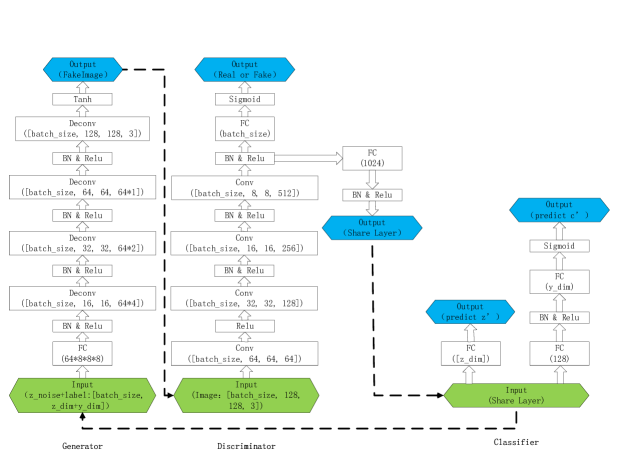
Figure 3: The overview of the network architecture of iterative GAN.

Iterative GAN includes three neural networks. The generator consists a fully-connected layer with 8584 neurons, four de-convolutional layers and each has 256, 128, 64 and 3 channels with filer size 5*5. All filter strides of the generator $\mathbf{G}$ are set as 2*2. After processed by the first fully-connected layer, the input noise $\mathbf{z}$ with 100 dimensions is projected and reshaped to [Batch_size, 5, 5, 512], the following 4 deconvolutional layers then transpose the tensor to [Batch_size, 16, 16, 256], [Batch_size, 32, 32, 128], [Batch_size, 64, 64, 64], [Batch_size, 128, 128, 3], respectively. The tensor output from the last layer is activated by the tanh function.

The discriminator is organized almost in the reverse way of the generator. It includes 4 convolutional layers with filter size 5*5 and stride size 2*2. The training images with shape [Batch_size, 128, 128, 3] then transpose through the following 4 convolutional layers and receive a tensor with shape [Batch_size, 5, 5, 512]. The discriminator needs to output two results, a shared layer for the classifier and probability that indicates if the input image is a fake one. We flat the tensor and pass it to classifier as input for the former purpose. To get the reality of image, we make an extra full connect layer which output [Batch_size, 1] shape tensor with sigmoid active function.

The classifier receives the shared layer from the discriminator which contains enough feature information. We build two full-connected layers in the classifier, one for the predicted noise $\tilde{\mathbf{z}}$ and the other for the output predicted labels $\tilde{\mathbf{c}}$. And we use the tanh and sigmoid function to squeeze the value $\tilde{\mathbf{z}}$ to (-1,1), $\tilde{\mathbf{c}}$ to (0, 1) respectively. And the Fig. 3 shows how we organize the networks of iterative GAN.

Table 1: Analysis of time consumption for training.

	epoch	image Size	cost time
Training	10	128*128	106,230 sec
	20	128*128	23,9460 sec
	50	128*128	600,030 sec

Table 2: Analysis of time consumption for testing.

	image num	input image size	output image size	cost time
Rebuild	64	128*128	128*128	3.2256 sec
Generate	64	$\backslash$	128*128	2.1558 sec

4.1 Optimization

Following the DCGAN radford2016unsupervised , we adopt the Adam optimizer adam2015ICLR to train proposed iterative GAN. The learning rate $\alpha$ is set to 0.0002 and $\beta_{1}$ is set to 0.5, $\beta_{2}$ is 0.999 (same settings as DCGAN). To avoid the imbalanced optimization between the 2 competitors G and D, which happened commonly during GANs’s training and caused the vanishment of gradients, we set 2 more parameters to control the update times of D and G in each iteration. While the loss of D is overwhelmingly higher than G, we increase the update times of D in this iteration, and vice versa. By using this trick, the stability of training process is apparently approved.

4.2 Statistics for Training and Testing

We introduce the time costs of training and testing in this section. The proposed iterative GAN model was trained on an Intel Core i5-7500 CPU@3.4GH_z with 4 cores and NVIDIA 1070Ti GPU. The training process goes through 50 epochs and shows the final results. The Analysis of the time consumption (including both training and forward propagation process) are shown in Table 1 and Table 2 respectively.

5 Experiment

We perform our experiment for multiple tasks to verify the capability of iterative GAN model: recognition of facial attributes, face images reconstruction, face transformation, and face generation with controllable attributes.

5.1 Dataset

We run the iterative GAN model on celebA dataset liu2015faceattributes which is based on celebFace+ sun2014deep . celebA is a large-scale face image dataset contains more than 200k samples of celebrities. Each face contains 40 familiar attributes, such as Bags_Under_Eyes, Bald, Bangs, Blond_Hair, etc. Owing to the rich annotations per image, celebA has been widely applied to face visual work like face attribute recognition, face detection, and landmark (or facial part) localization. We take advantage of the rich attribute annotations and train each label in a supervised learning approach.

We split the whole dataset into 2 subsets: 185000 images of them are randomly selected as training data, the remaining 15000 samples are used to evaluate the results of the experiment as the test set.

We crop the original images of size 178 * 218 into 178 * 178, then further resize them to 128 * 128 as the input samples. The size of the output (generated) images are as well as the inputs.

5.2 The Metric of Face Identity

Given a face image, whatever rebuilding it or transforming it with customized attributes, we have to preserve the similarity (or identity) between the input and output faces. It is very important for human face operation because the maintenance of the primary features belong to the same person is vital during the process of face transformation. Usually, the visual effect of face identity-preserving can only be observed via naked eyes.

Besides visual observation, in this paper, we choose FaceNet schroff2015facenet: to define the diversity between a pair of images. In particular, FaceNet accepts two images as input and output a score which reveal the similarity. A lower score indicates that the two images are more similar, and vice versa. In other words, FaceNet provides us a candidate metric on the face identity evaluation. We take it as an important reference in the following related experiments.

5.3 Results

5.3.1 Recognition of facial attributes (multi-labels)

Learning face attributes is fundamental to face generation and transformation. Previous work learned to control single attribute li2017generate or multi-category attributes Odena2017Conditional through a softmax function for a given input image. However, the natural face images are always associated with multiple labels. To the best of our knowledge, recognizing and controling the multi-label attributes for a given facial image are among most challenging issues in the community. In our framework, the classifier $\mathbf{C}$ accepts a 1024 dimensions shared vector that outputted by the discriminator $\mathbf{D}$, then $\mathbf{C}$ squash it into 128 dimensions by a full connection. To output the multiple labels, we just need to let the classifier $\mathbf{C}$ to compress the 128 dimension median vector into $d$ dimensions (as shown in Fig. 3, $d$ is the dimension of label vector, $d=40$ in this paper). By linking the $d$ dimensions vector to $d$ $sigmoid$ mappings, the classifier $\mathbf{C}$ output the predictions of attribute labels finally.

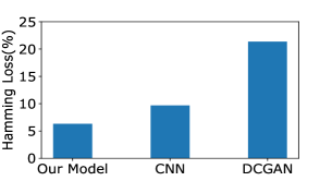
Figure 4: The hamming loss of attribute prediction.

We feed the images in test set to the classifier $\mathbf{C}$ and calculate the hamming loss for the multi-label prediction. The statistic of hamming loss is over all the 40 labels associated with each test samples. Two methods are selected as baselines. The first one is native DCGAN with L2-SVM classifier which is reported superior to $k$-means and $k$-NN radford2016unsupervised . The other is a Convolutional Neural Network. We train both referenced models on celebA. For the DCGAN, the discriminator extracts the features and feeds it to the linear L2-SVM with Euclidean distance for unsupervised classification. Mean while, the CNN model outputs the predicted labels directly after standard process of convolution training.

Fig. 4 illustrates the hamming loss of the three algorithms. It is clear to see that the iterative GAN significantly outperforms DCGAN+L2-SVM and CNN. We speculate that the proposed joint architecture on both face generation and transformation regularized by the integrated loss make the facial attribute learning of iterative GAN is much easier than the baselines.

Besides the hamming loss statistics of hamming loss, we also visualize part of the results in Table 3. Row 2, 3 and 4 in Table 3 illustrate three examples in the test set. Row 2 and 3 are the successful cases, while row 4 shows a failed case on predicting HeavyMakeUp and Male.

Target Image	Attribute	Truth	Prediction
	Bald	-1	0.0029
	Bangs	-1	0.0007
	BlackHair	1	0.8225
	BlondeHair	-1	0.2986
	EyeGlass	-1	0.0142
	Male	1	0.8669
	Nobeard	1	0.7255
	Smiling	1	0.9526
	WaveHair	1	0.6279
	Young	1	0.6206
	Attractive	1	0.7758
	Bald	-1	0.1826
	Male	-1	0.00269
	Smiling	1	0.7352
	HeavyMakeUp	1	0.5729
	Wearinghat	1	0.7699
	Young	1	0.8015
	Attractive	-1	0.4629
	Bald	-1	0.6397
	EyeGlass	1	0.8214
	HeaveMakeUp	-1	0.7566
	Male	1	0.3547

Table 3: Demonstrate the example of classification result of iterative GAN. The listed ground-truth tags of target image are expressed by two integer 1 and -1. Row 1 and 2 show the exactly correct prediction examples. Row 3 demonstrates the miss-classification example: the classifier failed to determine the attribute Heavy_makeup and Male of the face which expressed in black font.

5.3.2 Reconstruction

In this experiment, we reconstruct given target faces in 4 different settings (per-pixel_loss,$\mathbf{z}$_loss, $\mathbf{z}$_loss+per-pixel_loss, and the integrated Loss) separately. This experiment proves that the iterative GAN provided with integrated loss has a strong ability to deal with the duties mentioned above and archive the similar or better results than previous works.

By feeding the noise vector $\tilde{\mathbf{z}}$ and $\tilde{\mathbf{c}}$, the generator $\mathbf{G}$ can reconstruct the original input image with its attributes preserved ($\mathbf{x}_{\text{rebuilt}}$ in Fig. 2). We will evaluate the contributions of integrated loss in this experiment of face reconstruction. In detail, we run 4 experiments by regularizing the ACGAN Loss with: only per-pixel loss, latent code loss($\mathbf{z}$_loss), latent code loss($\mathbf{z}$_loss) + per-pixel loss, and latent code loss($\mathbf{z}$_loss) + per-pixel loss + perceptual loss.

The comparisons among the results of the 4 experiments are shown in Fig. 5. The First column displays the original images to be rebuilt. The remains are corresponding to the 4 groups of experiments mentioned before.

From column 2 to column 5, we have three visual observations:

• latent code loss ($\mathbf{z}$_loss) prefers to preserve image quality (images reconstructed with per-pixel loss in column 2 are blurrier than images reconstructed with only the latent code loss in the 3rd column) because the calculation of per-pixel loss over the whole pixel set flattens the image;

• images reconstructed with per-pixel loss, latent code loss, latent code loss + per-pixel loss all failed on preserving the face identity;

• the integrated loss benefits the effects of its three components that reconstruct the original faces with high quality and identity-preserving.

FaceNet also calculates an identity-preserving score for each rebuild face as shown in Fig. 5 (from column 2 to column 5). A smaller score indicates a closer relationship between two images. The scores from column 2 to column 5 demonstrate that the faces reconstructed by the integrated loss preserve better facial identity than the faces rebuild with other losses (column 2 to 4) in most of the cases. In other words, the integrated loss not only has an advantage on produce high-quality image but also can make a good facial identity-preserving. These experiments prove that the iterative GAN provided with integrated loss has a strong ability to deal with the tasks mentioned above and archives similar or better results than previous work.

\begin{overpic}[scale={0.4}]{reconstruction.pdf} \put(6.0,95.0){{\footnotesize Target}} \put(21.0,95.0){{\footnotesize per-pixel\_loss}} \par\put(45.0,95.0){{\footnotesize$\mathbf{z}$\_loss}} \par\put(58.0,95.0){{\footnotesize per-pixel\_loss}} \put(68.0,97.5){{\footnotesize+}} \put(65.0,100.0){{\footnotesize$\mathbf{z}$\_loss}} \par\put(80.0,98.0){{\footnotesize integrated }} \put(84.0,95.0){{\footnotesize loss}} \par\put(25.0,74.5){{\scriptsize 0.8669}} \put(45.0,74.5){{\scriptsize 0.8220}} \put(64.0,74.5){{\scriptsize 0.8857}} \put(83.0,74.5){{\scriptsize{0.5314}}} \par\put(25.0,55.0){{\scriptsize 0.7855}} \put(45.0,55.0){{\scriptsize 0.9658}} \put(64.0,55.0){{\scriptsize 0.7200}} \put(83.0,55.0){{\scriptsize{0.6089}}} \par\put(25.0,36.0){{\scriptsize 0.8521}} \put(45.0,36.0){{\scriptsize 0.7803}} \put(64.0,36.0){{\scriptsize 0.6086}} \put(83.0,36.0){{\scriptsize{0.5217}}} \par\put(25.0,17.0){{\scriptsize 0.9038}} \put(45.0,17.0){{\scriptsize 0.9311}} \put(64.0,17.0){{\scriptsize 0.7412}} \put(83.0,17.0){{\scriptsize{0.7259}}} \par\put(25.0,-2.5){{\scriptsize 0.7041}} \put(45.0,-2.5){{\scriptsize 0.8588}} \put(64.0,-2.5){{\scriptsize 0.6779}} \put(83.0,-2.5){{\scriptsize{0.4636}}} \par\par\end{overpic}

Figure 5: Comparison of rebuilding images through different losses. The first column shows the original nature-image. The 2nd and 3rd columns are images rebuilt with only per-pixel loss or $\mathbf{z}$_loss (latent code). Column 4 shows the effect of $\mathbf{z}$_loss + pixel_loss effect. The last column shows the final effect of the integrated loss. The FaceNet scores below each image in 2nd to 5th columns reveals the distance from the target image. Images rebuild from integrated loss(the last column) get the smallest score(expressed in black font).

5.3.3 Face Transformation with Controllable Attributes

Based on our framework, we feed the discriminator $\mathbf{D}$ a real image without its attribute labels $\mathbf{c}$, then we get a noise representation $\tilde{\mathbf{z}}$ and label vector $\tilde{\mathbf{c}}$ from $\mathbf{C}$ as output. We can reconstruct the original image with $\tilde{\mathbf{z}}$ and $\tilde{\mathbf{c}}$ as we did in Section 5.3.2. Alternatively, we can transform the original image into another one by customizing its attributes in $\tilde{\mathbf{c}}$. By modifying part or even all labels of $\tilde{\mathbf{c}}$, the corresponding attributes of the reconstructed image will be transformed.

In this section, we study the performance of image transformation of our model. We begin the experiments with controlling a single attribute. That is, to modify one of the attributes of the images on the test set. Fig. 6 shows the part of the results of the transformation on the test set. The four rows of Fig. 6 illustrate four different attributes Male, Eye_Glasses, Bangs, Bald have been changed. The odd columns display the original images, and even columns illustrate the transformed images. We observe that the transformed images preserve high fidelity and their old attributes.

Finally, we extend it to the attribute manipulation from the single case to the multi-label scenario. Fig. 7 exhibits the results manipulating multiple attributes. The first column is the target faces. Faces in column 2 are the corresponding ones that reconstructed by iterative GAN (no attributes have been modified). The remaining 5 columns display the face transformation (column 3,4,5: single attribute; column 6,7: multiple attributes). For these transformed faces, we observe that both the image quality and face identity preserving are well satisfied. As we see, for the multi-label case, we only modified 3 attributes in the test. Actually, we have tried to manipulate more attributes (4-6) one time while the image quality drastically decreased. There is a lot of things to improve and we left it as the future work.

\begin{overpic}[scale={0.6}]{Single.pdf} \put(3.0,39.0){{\footnotesize Male}} \put(2.0,29.0){{\footnotesize Glasses}} \put(2.0,19.0){{\footnotesize Bangs}} \put(3.0,8.5){{\footnotesize Bald}} \end{overpic}

Figure 6: Four examples (male, glasses, bangs, and bald as shown in the four rows) of face transformation with a single attribute changing. For each example (row), we display five illustrations. For instance, the first row shows the results of controlling the label of the male. The odd columns of row 1 are the given faces, the corresponding even columns display the faces with male reversed. From the 1st and 5th instances (columns 1,2 and 9,10), we clearly see that the mustache disappeared from male to female.

\begin{overpic}[scale={0.55}]{attri2.pdf} \put(2.5,95.3){{\tiny Target}} \put(12.5,95.3){{\tiny Rebuild}} \put(21.5,95.3){{\tiny Reversal:Bangs}} \put(31.5,95.3){{\tiny Reversal:Glasses}} \put(42.5,95.3){{\tiny Reversal:Male}} \put(53.7,95.3){{\tiny Reversal:Bangs}} \put(53.7,96.6){{\tiny Reversal:Glasses}} \put(64.6,95.3){{\tiny Reversal:Male}} \put(64.6,96.6){{\tiny Reversal:Bangs}} \end{overpic}

Figure 7: Demonstrations of rebuilding the target images and reversing (modifying) some attributes of the original face simultaneously. The first column shows the target face. The rebuilt faces are shown in the 2nd column with all attributes unchanged. Then we reverse the 3 single labels successively from 3rd column to the 7th column. For example, the target face has the attribute ’Bangs’ (column 3), we reverse the corresponding label ’Bangs’ to eliminate this attribute and keep others fixed. The last 2 columns show the combination of attributes modification.

5.3.4 Compare with Existing Method of Image Transformation

Image transformation puts the emphases on finding a way to map the original image to an output image which subjects to another different domain. Editing the image attributes of a person is a special topic in this area. One of the popular methods attracted lots of attention recently is the CycleGAN Zhu2017Unpaired . The key point of CycleGAN is that it builds upon the power of the PIX2PIX denoord2016conditional architecture, with discrete, unpaired collections of training images.

In this experiment, we compare CycleGAN with iterative GAN on face transformation. We randomly select three facial attributes the Bangs ,Glasses, and Bald for testing.

For CycleGAN, we split the training dataset into 2 groups for each of the three attributes. For example, to train CycleGAN with the Bangs, we divide the images into 2 sets, faces with bangs belong to domain 1 and the ones without bangs belong to domain 2. According to the results shown in Figure 9 $(a)$, we found that CycleGAN is insensitive to the geometry transformation though it did a good job in catching some different features between two domains like color. As we know, CycleGAN is good at transforming the style of an image, for example, translate a horse image to zebra one Zhu2017Unpaired . For the test of human faces, however, it fails to recognize and manipulate the three facial attributes Bangs ,Glasses, and Bald as shown in column 2 of Fig. 9 $(a)$. By contrast, the iterative GAN achieves better results in transforming the same face with one attribute changed and others preserved.

5.3.5 Face Generation with Controllable Attributes

Different from above, we can also generate a new face with a random $\mathbf{z}$ sampling from a given distribution and an artificial attribute description $\mathbf{c}$ (labels). The generator $\mathbf{G}$ accepts $\mathbf{z}$ and $\mathbf{c}$ as the inputs and fabricates a fictitious facial image $\mathbf{x}_{\text{fake}}$ as the output. Of course, we can customize an image by modifying the corresponding attribute descriptions in $\mathbf{c}$. For example, the police would like to get a suspect’s portrait by the witness’s description “He is around 40 years old bald man with arched eyebrows and big nose”.

\begin{overpic}[scale={0.5}]{generate.pdf} \put(-3.0,35.4){{\scriptsize Random build from}} \put(0.0,33.5){{\scriptsize$\mathbf{z}\sim U(-1,1)$}} \par\par\put(24.0,70.0){{\tiny+Bush\_Eyebrows}} \par\put(38.0,70.0){{\tiny+Glasses}} \par\put(48.0,70.0){{\tiny+Smiling}} \par\put(58.0,70.0){{\tiny+Bangs}} \put(58.0,71.8){{\tiny+Bush\_Eyebrows}} \par\put(70.0,70.0){{\tiny+Bangs}} \put(70.0,71.8){{\tiny+Bush\_Eyebrows}} \put(70.0,73.6){{\tiny+Glasses}} \par\par\par\end{overpic}

Figure 8: Demonstration of building faces.The 1st column is faces build from random noise $\mathbf{z}$ which is sampled from the Uniform distribution. The 2nd to 4th columns show the standard faces created with the noise vector $\mathbf{z}$ plus single label such as Bush_Eyebrows, Glasses, Smiling. The left 2 columns are the examples of manipulating multiple attributes.

Fig. 8 illustrates the results of generating fictitious facial images with random noise and descriptions. We sample $\mathbf{z}$ from the Uniform distribution. The first column displays the images generated with $\mathbf{z}$ and initial descriptions. The remaining columns demonstrate the facial images generated with modified attributes (single or multiple modifications).

5.3.6 Compare with Existing Method of Face Generation

To examine the ability to generate realistic facial images of the proposed model, we compare the results of face generation of the proposed model with two baselines, the CGAN Mirza2014Conditional and ACGAN Odena2017Conditional respectively. These three models can all generate images with a conditioned attributes description. For each of them, we begin the experiment by generating random facial images as illustrated in the 1st, 3rd, and 5th column of Fig. 9, part $(b)$, respectively. The column 2, 4, and 6 display the generated images with the 3 attributes (Bangs, Glasses, Bald modified for CGAN, ACGAN, and our model. It is clear to see that the face quality of our model is better than CGAN and ACGAN. And most importantly, in contrast with the failure of preserving face identity (see Fig. 9 $(b)$, the intersections between column 3, 4 and row 1 of ACGAN, column 1, 2 and row 2, 3 of CGAN), our model can always perform the best in face identity preserving.

\begin{overpic}[scale={0.48}]{compareOtherGAN.jpg} \put(2.0,40.0){{\footnotesize Target}} \put(12.0,40.0){{\footnotesize CycleGAN}} \put(22.5,40.0){{\footnotesize iterative GAN}} \par\put(46.0,40.0){{\footnotesize CGAN}} \put(66.0,40.0){{\footnotesize AC-GAN}} \put(84.0,40.0){{\footnotesize iterative GAN}} \par\put(-6.0,34.0){{\footnotesize Bangs}} \put(-6.5,20.5){{\footnotesize Glasses}} \put(-5.0,8.0){{\footnotesize Bald}} \par\put(15.0,27.0){{\scriptsize 0.6749 }} \put(26.0,27.0){{{0.5520} }} \par\put(48.0,27.0){{\scriptsize 0.7432 }} \put(68.0,27.0){{\scriptsize 1.0794 }} \put(88.0,27.0){{{0.6066} }} \par\put(15.0,14.5){{{0.4480} }} \put(26.0,14.5){{\scriptsize 0.5871 }} \par\put(48.0,14.5){{\scriptsize 1.2572 }} \put(68.0,14.5){{\scriptsize 0.5520 }} \put(88.0,14.5){{{0.5128} }} \par\put(15.0,1.7){{\scriptsize 0.6112 }} \put(26.0,1.7){{{0.6069} }} \par\put(48.0,1.7){{\scriptsize 0.7831 }} \put(68.0,1.7){{\scriptsize 0.6928 }} \put(88.0,1.7){{{0.5434} }} \par\par\put(21.0,-1.0){{\footnotesize$(a)$}} \put(70.0,-1.0){{\footnotesize$(b)$}} \par\end{overpic}

Figure 9: Comparing with iterative GAN and other GANs on face generation and transformation. Part $(a)$ shows the results of transforming given images to another with facial attributes changed. When Cycle GAN is performed,the quality of output is so poor since Cycle GAN seems to insensitive to the subtle changes of facial attributes and even failed in some labels(see the image in row 3 column 2). Part $b$ compared the capability of generating an image with iterative GAN and CGAN, AC-GAN. The result shows that our model can produce the desired image with comparable or even better quality than AC-GAN, and far better than native CGAN. More importantly, according to the FaceNet scores(below each output image), it seems clear that the proposed iterative architecture has an advantage of preserving facial identity.

It is clear to see that the face quality of ACGAN and our model is much better than CGAN. And most importantly, in contrast with the failure of preserving face identity (see the intersections between column 3, 4 and row 1, 2 of ACGAN), our model can always make a good face identity-preserving.

In summary, extensive experimental results indicate that our method is capable of: 1)recognizing facial attribute; 2)generating high-quality face images with multiple controllable attributes; 3)transforming an input face into an output one with desired attributes changing; 4)preserving the facial identity during face generation and transformation.

6 Conclusion

We propose an iterative GAN to perform face generation and transformation jointly by utilizing the strong dependency between the face generation and transformation. To preserve facial identity, an integrated loss including both the per-pixel loss and the perceptual loss is introduced in addition to the traditional adversarial loss. Experiments on a real-world face dataset demonstrate the advantages of the proposed model on both generating high-quality images and transforming image with controllable attributes.

- (1) Berg, T., Belhumeur, P.N.: Poof: Part-based one-vs.-one features for fine-grained categorization, face verification, and attribute estimation pp. 955–962 (2013)
- (2) Bettadapura, V.: Face expression recognition and analysis: The state of the art. Tech Report, arXiv:1203.6722 (2012)
- (3) Bourdev, L.D., Maji, S., Malik, J.: Describing people: A poselet-based approach to attribute classification pp. 1543–1550 (2011)
- (4) Branson, S., Wah, C., Schroff, F., Babenko, B., Welinder, P., Perona, P., Belongie, S.J.: Visual recognition with humans in the loop pp. 438–451 (2010)
- (5) Cherniavsky, N., Laptev, I., Sivic, J., Zisserman, A.: Semi-supervised learning of facial attributes in video pp. 43–56 (2010)
- (6) Cortes, C., Vapnik, V.: Support-vector networks. Machine Learning 20(3), 273–297 (1995)
- (7) Dalal, N., Triggs, B.: Histograms of oriented gradients for human detection 1, 886–893 (2005)
- (8) Den Oord, A.V., Kalchbrenner, N., Vinyals, O., Espeholt, L., Graves, A., Kavukcuoglu, K.: Conditional image generation with pixelcnn decoders. neural information processing systems pp. 4790–4798 (2016)
- (9) Denton, E.L., Chintala, S., Szlam, A., Fergus, R.D.: Deep generative image models using a laplacian pyramid of adversarial networks. neural information processing systems pp. 1486–1494 (2015)
- (10) Dong, C., Loy, C.C., He, K., Tang, X.: Learning a deep convolutional network for image super-resolution pp. 184–199 (2014)
- (11) Dosovitskiy, A., Brox, T.: Generating images with perceptual similarity metrics based on deep networks. neural information processing systems pp. 658–666 (2016)
- (12) Farhadi, A., Endres, I., Hoiem, D., Forsyth, D.: Describing objects by their attributes. In: Computer Vision and Pattern Recognition, 2009. CVPR 2009. IEEE Conference on, pp. 1778–1785 (2009)
- (13) Gatys, L.A., Ecker, A.S., Bethge, M.: A neural algorithm of artistic style. Nature Communications (2015)
- (14) Gauthier, J.: Conditional generative adversarial nets for convolutional face generation. Class Project for Stanford CS231N: Convolutional Neural Networks for Visual Recognition (Winter semester 2014)
- (15) Goodfellow, I.J., Pougetabadie, J., Mirza, M., Xu, B., Wardefarley, D., Ozair, S., Courville, A.C., Bengio, Y.: Generative adversarial nets pp. 2672–2680 (2014)
- (16) Gregor, K., Danihelka, I., Graves, A., Rezende, D.J., Wierstra, D.: Draw: A recurrent neural network for image generation. international conference on machine learning pp. 1462–1471 (2015)
- (17) Isola, P., Zhu, J.Y., Zhou, T., Efros, A.A.: Image-to-image translation with conditional adversarial networks (2016)
- (18) Johnson, J., Alahi, A., Feifei, L.: Perceptual losses for real-time style transfer and super-resolution. european conference on computer vision pp. 694–711 (2016)
- (19) Kingma, D., Ba, J.: Adam: A method for stochastic optimization. In: International Conference on Learning Representation (2015)
- (20) Kingma, D.P., Rezende, D.J., Mohamed, S., Welling, M.: Semi-supervised learning with deep generative models. Advances in Neural Information Processing Systems 4, 3581–3589 (2014)
- (21) Kingma, D.P., Welling, M.: Auto-encoding variational bayes. international conference on learning representations (2014)
- (22) Kumar, N., Berg, A.C., Belhumeur, P.N., Nayar, S.K.: Attribute and simile classifiers for face verification pp. 365–372 (2009)
- (23) Larsen, A.B.L., Sonderby, S.K., Larochelle, H., Winther, O.: Autoencoding beyond pixels using a learned similarity metric. international conference on machine learning pp. 1558–1566 (2016)
- (24) Ledig, C., Theis, L., Huszar, F., Caballero, J., Cunningham, A., Acosta, A., Aitken, A.P., Tejani, A., Totz, J., Wang, Z., et al.: Photo-realistic single image super-resolution using a generative adversarial network. computer vision and pattern recognition pp. 4681–4690 (2016)
- (25) Li, Z., Luo, Y.: Generate identity-preserving faces by generative adversarial networks. arXiv preprint arXiv:1706.03227 (2017)
- (26) Liu, Z., Luo, P., Wang, X., Tang, X.: Deep learning face attributes in the wild. In: Proceedings of International Conference on Computer Vision (ICCV), pp. 3730–3738 (2015)
- (27) Mcquistonsurrett, D., Topp, L.D., Malpass, R.S.: Use of facial composite systems in us law enforcement agencies. Psychology Crime & Law 12(5), 505–517 (2006)
- (28) Mirza, M., Osindero, S.: Conditional generative adversarial nets. Computer Science pp. 2672–2680 (2014)
- (29) Nilsback, M., Zisserman, A.: Automated flower classification over a large number of classes pp. 722–729 (2008)
- (30) Odena, A., Olah, C., Shlens, J.: Conditional image synthesis with auxiliary classifier gans (2017)
- (31) Parikh, D., Grauman, K.: Relative attributes (2011)
- (32) Radford, A., Metz, L., Chintala, S.: Unsupervised representation learning with deep convolutional generative adversarial networks. International Conference on Learning Representations (2016)
- (33) Schroff, F., Kalenichenko, D., Philbin, J.: Facenet: A unified embedding for face recognition and clustering. computer vision and pattern recognition pp. 815–823 (2015)
- (34) Shu, Z., Yumer, E., Hadap, S., Sunkavalli, K., Shechtman, E., Samaras, D.: Neural face editing with intrinsic image disentangling. CoRR abs/1704.04131 (2017). URL http://arxiv.org/abs/1704.04131
- (35) Simonyan, K., Zisserman, A.: Very deep convolutional networks for large-scale image recognition. international conference on learning representations (2015)
- (36) Sun, Y., Chen, Y., Wang, X., Tang, X.: Deep learning face representation by joint identification-verification. neural information processing systems pp. 1988–1996 (2014)
- (37) Szegedy, C., Liu, W., Jia, Y., Sermanet, P., Reed, S.E., Anguelov, D., Erhan, D., Vanhoucke, V., Rabinovich, A.: Going deeper with convolutions. computer vision and pattern recognition pp. 1–9 (2015)
- (38) Tatarchenko, M., Dosovitskiy, A., Brox, T.: Multi-view 3d models from single images with a convolutional network. european conference on computer vision pp. 322–337 (2016)
- (39) Wang, C., Wang, C., Xu, C., Tao, D.: Tag disentangled generative adversarial network for object image re-rendering. In: Twenty-Sixth International Joint Conference on Artificial Intelligence, pp. 2901–2907 (2017)
- (40) Wang, C., Xu, C., Wang, C., Tao, D.: Perceptual adversarial networks for image-to-image transformation (2017)
- (41) Wang, X., Gupta, A.: Generative image modeling using style and structure adversarial networks. european conference on computer vision pp. 318–335 (2016)
- (42) Xie, J., Xu, L., Chen, E.: Image denoising and inpainting with deep neural networks pp. 341–349 (2012)
- (43) Yan, X., Yang, J., Sohn, K., Lee, H.: Attribute2image: Conditional image generation from visual attributes. european conference on computer vision pp. 776–791 (2015)
- (44) Yoo, D., Kim, N., Park, S., Paek, A.S., Kweon, I.S.: Pixel-level domain transfer. european conference on computer vision pp. 517–532 (2016)
- (45) Zhang, N., Paluri, M., Ranzato, M., Darrell, T., Bourdev, L.D.: Panda: Pose aligned networks for deep attribute modeling. computer vision and pattern recognition pp. 1637–1644 (2014)
- (46) Zhang, R., Isola, P., Efros, A.A.: Colorful image colorization. european conference on computer vision pp. 649–666 (2016)
- (47) Zhang, Z., Song, Y., Qi, H.: Age progression/regression by conditional adversarial autoencoder. arXiv preprint arXiv:1702.08423 (2017)
- (48) Zhu, J., Krahenbuhl, P., Shechtman, E., Efros, A.A.: Generative visual manipulation on the natural image manifold. european conference on computer vision pp. 597–613 (2016)
- (49) Zhu, J.Y., Park, T., Isola, P., Efros, A.A.: Unpaired image-to-image translation using cycle-consistent adversarial networks (2017)