Abstract

The Type-II seesaw model is a well-motivated new physics scenario to address the origin of the neutrino mass issue. We show that this model can easily accommodate an absolutely stable vacuum until the Planck scale, however with strong limit on the exotic scalar masses and the corresponding mixing angle. We examine the model prediction at the current and future high luminosity run of the Large Hadron Collider (LHC) for the scalar masses and mixing angles fixed at such high-scale valid region. Specifically, we device the associated and pair production of the charged scalars as a new probe of the model at the LHC. We show that for a particular signal process the model can be tested with $5\sigma$ signal significance even at the present run of the LHC.

I Introduction

The discovery of the 125 GeV resonance at the Large Hadron Collider (LHC) [1, 2] with its increasing biasness towards the Standard Model (SM) values for couplings, anyway, has set forth one of the most discussed questions of this time that asks for an absolute stable electroweak vacuum up to very high scale, say Grand Unification Scale (GUT) $(10^{16}~{}\rm GeV)$ or Planck Scale $(10^{19}~{}\rm GeV)$. The evolution of the Higgs quartic coupling only with SM interaction, is unable to maintain its boundedness from below much before the GUT or Planck scale and becomes negative at around $10^{10}~{}\rm GeV$ even after taking into account all the uncertainties in determining the top quark mass and strong coupling constant  [3, 4, 5, 6, 7, 8]. This subsequently calls for intervention of some new physics scenario at or before such scale. Although, a metastable vacuum could be a possibility, the quest for the absolute stability can be advocated for the hunt for new physics (NP) scenarios. To affirm the positivity of the Higgs quartic coupling all its way during the renormalization group (RG) evolution, positive aid from extra scalar bosons are mandatory to negotiate the negative fermionic pull that comes dominantly from the top quark. Therefore, NP models that extends the SM scalar sector can easily serve the purpose. In view of this, the triplet scalar extension, alias, the Type-II seesaw model has already been proven a well-deserved NP candidate to ameliorate the vacuum stability problem [9, 10, 11, 12, 13]. In order to seek an absolutely stable vacuum in the Type-II seesaw regime, one must also maintain the perturbative unitarity of all the new couplings introduced lately. It has been studied that all these stability and perturbative unitarity requirements together can dramatically control the allowed region of the model parameter space in view of the non-standard scalar masses and mixing even only at the electroweak (EW) scale [14, 15]. Nevertheless, a complete picture of the allowed parameter space in light of high-scale validity of this scenario in terms of the physical masses and mixing has not been emphasized before.

On a different note, the Type-II seesaw model [16, 17, 18, 19, 20, 21] has mainly been preferred for its attributes towards the generation of tiny nonzero neutrino masses through the seesaw mechanism. Unlike the other two variants of seesaw, Type-II does not inherit an extended fermion sector, rather it includes an extra $SU(2)_{L}$ triplet scalar to the SM particle content and the lepton number is broken by two units through a trilinear coupling $(\mu)$ in the scalar potential. The neutrinos acquire Majorana mass term through the Yukawa interaction of these triplet with the lepton doublets and the small neutrino masses are proportional to the product of the Yukawa couplings $(Y_{\Delta})$ and the trilinear coupling $(\sim{Y_{\Delta}\mu v_{d}^{2}}/{M_{\Delta}^{2}})$ where, $M_{\Delta}$ is the triplet scalar mass parameter and $v_{d}$ is the SM vacuum expectation value (vev). The smallness of the neutrino mass can thus be translated by the trilinear coupling $\mu$, which is protected by symmetry and can be small following the t’hooft’s naturalness criterion [22]. In fact, this $\mu$ term is responsible for the vev of the triplet ($v_{t}$) as it yields the tadpole term for the scalar triplet due to the spontaneous electroweak symmetry breaking (EWSB) as $v_{t}\sim({\mu v_{d}^{2}}/{M_{\Delta}^{2}})$. In general, a proper tuning between these two parameters ($\mu$ or $v_{t}$ and $Y_{\Delta}$) in accordance with the current neutrino oscillation data [23] can generate the tiny neutrino masses even keeping the newly introduced scalar masses around the EW scale $(M_{\Delta}\sim v_{d})$ unlike the other two types of seesaw mechanisms where the new fermion masses necessarily has large values ($10^{9}-10^{10}~{}\rm GeV$). Therefore, the exotic triplet scalars of Type-II seesaw models lie in the reach of the current collider experiments which makes this particular seesaw type to be phenomenologically more appealing. In addition, the presence of both singly and doubly charged scalars make this model very attractive from the point of view of exotic particles search at the colliders.

In this work, we rekindle the idea of probing the Type-II seesaw model parameter space at the LHC that are conclusively allowed by all the stability and perturbativite unitarity requirements until the Planck scale. The search strategy could thus be restrictive as the extra theoretical constraints have put stringent bound on the non standard scalar mass splitting. The splitting between the singly and doubly charged scalar masses is also tuned by the one-loop T-parameter constraint at the EW scale [9, 24]. It is therefore expected that the allowed parameter region in the high-scale valid space will be more contrived. Moreover, to have the lightest CP-even state as the 125 GeV resonance state with the SM-Higgs like coupling, one must ensure that the signal strengths for various decay modes do not overshoot the current experimental limit. In this scenario only the loop induced decay mode of the Higgs boson, $h\to\gamma\gamma$[25, 26] can be affected due to the presence of extra singly and doubly charged scalars and hence it is important to consider the limit on the corresponding signal strength ($\mu_{\gamma\gamma}$) as an additional constrain.

The triplet vev $(v_{t})$ plays a crucial role in this model. The value of $v_{t}$ is highly constrained by the $\rho$-parameter and quantitatively it can not be larger than a few GeV [27]. This has a greater implication on the decay modes of the singly and doubly charged scalars. To be specific, for $v_{t}<10^{-4}~{}\rm GeV$, the triplet scalars dominantly decay into leptonic final state and for $v_{t}>10^{-4}~{}\rm GeV$, only gauge boson final states or cascade decays of charged scalars (if they are kinematically allowed) are possible [28, 29, 30]. The latest same-sign dilepton searches at the LHC have already put strong lower limit on doubly charged scalar mass ($>$ 770 - 800 GeV) [31]. However, this limit is only valid for $v_{t}<10^{-4}~{}\rm GeV$ when the doubly charged scalar decays to dilepton pair with $100\%$ branching ratio. The collider search becomes more involved for $v_{t}\sim 1~{}\rm GeV$, due to more complicated decay patterns of the singly and doubly charged scalars. As a result, the lower bounds on these scalars are very relaxed. Some collider analyses for this case have been done before  [32, 33, 34, 35, 36] and after [37, 38, 39, 40, 41, 42, 43, 44] the Higgs discovery but our analysis goes beyond what has been reported so far. In our analysis, we demonstrate the complete picture of a high-scale valid Type-II seesaw potential and analyze the signal significance at the LHC in the allowed parameter space. To be specific, for collider study, we pursue the two different final state topologies, $3\ell^{\pm}+E_{T}/\;\>$ and $2\ell^{\pm}+4j+E_{T}/\;\>$, where, $\ell\equiv e,\mu$. The first channel ($3\ell^{\pm}+E_{T}/\;\>$) comes from the associate production of the singly and doubly charged scalars, while the second channel ($2\ell^{\pm}+4j+E_{T}/\;\>$) gets contributions from the associated production as well as from the doubly charged scalar pair production process. Performing a cut-based analysis to reduce the SM background efficiently, we explore the possibility of probing the model parameter space in the current and high luminosity run of the 13 TeV LHC. Such comprehensive study in view of simultaneous consideration of high scale stability and collider prediction is completely new.

The paper is organised in the following way. In section II we discuss the model and set our conventions. Then we briefly discuss the various theoretical and experimental constraints applied on the model parameter space in section III. Following this, in section IV we describe the features of the model emerged from high scale stability requirement. Next, in section V we perform the collider analysis. Finally, we conclude in section VI.

II $Y=2$, Higgs Triplet Model in a nutshell

In this section, we briefly discuss the Type-II seesaw model. It contains an $SU(2)_{L}$ triplet scalar field $\Delta$ with hypercharge $Y=2$ in addition to the SM fields.

$$\Delta = \frac{\sigma^{i}}{\sqrt{2}}\Delta_{i}=\left(\begin{array}[]{cc}\delta^{+}/\sqrt{2}&\delta^{++}\\ \delta^{0}&-\delta^{+}/\sqrt{2}\end{array}\right),$$ (3)

where $\Delta_{1}=(\delta^{++}+\delta^{0})/\sqrt{2},~{}\Delta_{2}=i(\delta^{++}-\delta^{0})/\sqrt{2},~{}\Delta_{3}=\delta^{+}$. The complete Lagrangian of this scenario is given by:

$${\cal L}={\cal L}_{\rm Yukawa}+{\cal L}_{\rm Kinetic}-V(\Phi,\Delta),$$ (4)

where the kinetic and Yukawa interactions are respectively [45]

$${\cal L}_{\rm kinetic} = \left(D_{\mu}\Phi\right)^{\dagger}\left(D^{\mu}\Phi\right)+{\rm Tr}\left[\left(D_{\mu}\Delta\right)^{\dagger}\left(D^{\mu}\Delta\right)\right],$$ (5)

$${\cal L}_{\rm Yukawa} = {\cal L}_{\rm Yukawa}^{\rm SM}-\left(Y_{\Delta}\right)_{ij}L_{i}^{\sf T}Ci\sigma_{2}\Delta L_{j}+{\rm h.c.}\,.$$ (6)

Here $\Phi^{\sf T}=(\phi^{+}~{}~{}~{}\phi^{0})$ is the SM scalar doublet and $L$ represents $SU(2)_{L}$ left-handed lepton doublet. Neutrino Yukawa coupling is represented by $Y_{\Delta}$, and $C$ is the Dirac charge conjugation matrix. Covariant derivative of the scalar triplet field is given by:

$$D_{\mu}\Delta=\partial_{\mu}\Delta+i\frac{g}{2}[\sigma^{a}W_{\mu}^{a},\Delta]+ig^{\prime}B_{\mu}\Delta\qquad(a=1,2,3).$$ (7)

$\sigma^{a}$ are the Pauli matrices, $g$ and $g^{\prime}$ are the gauge coupling constants of the $SU(2)_{L}$ and $U(1)_{Y}$ group respectively.

The most general scalar potential is given as [45]:

$$V(\Phi,\Delta) = -m^{2}_{\Phi}(\Phi^{\dagger}\Phi)+\frac{\lambda}{4}(\Phi^{\dagger}\Phi)^{2}+M^{2}_{\Delta}{\rm Tr}(\Delta^{\dagger}\Delta)+\left(\mu\Phi^{\sf T}i\sigma_{2}\Delta^{\dagger}\Phi+{\rm h.c.}\right)+\,$$ (8)

$$\lambda_{1}(\Phi^{\dagger}\Phi){\rm Tr}(\Delta^{\dagger}\Delta)+\lambda_{2}\left[{\rm Tr}(\Delta^{\dagger}\Delta)\right]^{2}+\lambda_{3}{\rm Tr}(\Delta^{\dagger}\Delta)^{2}+\lambda_{4}\Phi^{\dagger}\Delta\Delta^{\dagger}\Phi.$$

All the parameters of the potential can be taken to be real without loss of generality. After the EWSB, the minimization of the potential calculates the two mass parameters as,

$$m_{\Phi}^{2}=\lambda\frac{v_{d}^{2}}{4}-\sqrt{2}\mu v_{t}+\frac{(\lambda_{1}+\lambda_{4})}{2}v_{t}^{2}\,,$$ (9)

$$M_{\Delta}^{2}=\frac{\mu v_{d}^{2}}{\sqrt{2}v_{t}}-\frac{\lambda_{1}+\lambda_{4}}{2}v_{d}^{2}-(\lambda_{2}+\lambda_{3})v_{t}^{2}\,,$$ (10)

where, $v_{d}$ and $v_{t}$ stands for the doublet and triplet vev respectively and the electroweak vev is given by $v=\sqrt{v_{d}^{2}+2v_{t}^{2}}=246~{}\rm GeV$. The triplet vev $(v_{t})$ contributes to the electroweak gauge boson masses $M_{W}^{2}$ and $M_{Z}^{2}$ at tree level, $M_{W}^{2}=\frac{g^{2}(v^{2}_{d}+2v^{2}_{t})}{4}$ and $M_{Z}^{2}=\frac{g^{2}(v^{2}_{d}+4v^{2}_{t})}{4\cos^{2}\theta_{W}}$ respectively, thus modifying the SM $\rho$-parameter as:

$$\rho=\frac{M_{W}^{2}}{M_{Z}^{2}\cos^{2}\theta_{W}}=\frac{1+\frac{2v_{t}^{2}}{v_{d}^{2}}}{1+\frac{4v_{t}^{2}}{v_{d}^{2}}}\,.$$ (11)

The electroweak precision data constraints require the $\rho$-parameter to be very close to its SM value of unity and from the latest data: $\rho=1.0004^{+0.0003}_{-0.0004}$ [46]. Consequently, one gets an upper bound on $\frac{v_{t}}{v_{d}}<0.02$ or $v_{t}<5$ GeV. Hence, the triplet vev $v_{t}$ remains much smaller than the doublet vev $v_{d}$. On the other hand, from minimization condition one gets $v_{t}\propto\frac{\mu v_{d}^{2}}{M_{\Delta}^{2}}$ which further contributes to the neutrino mass generation as $M_{\nu}=\sqrt{2}{v_{t}Y_{\Delta}}$. The mass matrix $M_{\nu}$ is diagonalized by the neutrino mixing matrix, i.e. Pontecorvo-Maki-Nakagawa-Sakata (PMNS) matrix, the components of which are determined by the neutrino oscillation data for a particular neutrino mass hierarchy (for further details, see  [11, 47]). Therefore, neutrino mass ${\cal O}(0.1)$ eV can be obtained by tuning either the triplet vev $(v_{t})$ or the Yukawa coupling $(Y_{\Delta})$. For $v_{t}\sim{\cal O}(~{}\rm GeV)$, the Yukawa coupling has to be small, while an order one neutrino Yukawa coupling $(Y_{\Delta}\sim{\cal O}(1))$, demands $v_{t}\sim{\cal O}(10^{-2}~{}\rm eV)$. This sets the two extreme limits of the triplet vev.

After EWSB, the scalar fields expanded around respective vevs, can be parametrized as

$$\Phi = \frac{1}{\sqrt{2}}\left(\begin{array}[]{c}\sqrt{2}\chi_{d}^{+}\\ v_{d}+h_{d}+i\eta_{d}\\ \end{array}\right)\qquad\Delta=\frac{1}{\sqrt{2}}\left(\begin{array}[]{cc}\delta^{+}&\sqrt{2}\delta^{++}\\ v_{t}+h_{t}+i\eta_{t}&-\delta^{+}\end{array}\right)\;.$$ (16)

As a consequence, the scalar spectrum contains seven physical Higgs bosons: two doubly charged $H^{\pm\pm}$, two singly charged $H^{\pm}$, two CP-even neural ($h,H$) and a CP-odd ($A$) Higgs particles. The mass matrix diagonalizations are done using orthogonal rotation matrices comprising of rotation angles $\alpha,\beta$ and $\beta^{\prime}$ respectively for the CP-even, CP-odd and charged sector.

The corresponding mixing angles are given as

$$\tan\beta^{\prime} = \frac{\sqrt{2}v_{t}}{v_{d}},\quad\tan\beta=\frac{2v_{t}}{v_{d}}\equiv\sqrt{2}\tan\beta^{\prime}$$ (17a)

$${\rm and}~{}~{}\tan{2\alpha} = \frac{2\mathcal{B}}{\mathcal{A}-\mathcal{C}},$$ (17b)

$${\rm where,}\quad\mathcal{A}=\frac{\lambda}{2}v_{d}^{2}, \mathcal{B}=v_{d}[-\sqrt{2}\mu+(\lambda_{1}+\lambda_{4})v_{t}],\quad\mathcal{C}=\frac{\sqrt{2}\mu v^{2}_{d}+4(\lambda_{2}+\lambda_{3})v^{3}_{t}}{2v_{t}}.$$ (17c)

From the scalar potential of Eq. (8) it is evident that there lies eight independent parameters. Among which the two bilinear terms $m_{\Phi}^{2}$ and $M_{\Delta}^{2}$ can be traded off for the two vevs $(v_{d},v_{t})$ using the minimization conditions given in Eqs. (9) and (10). The remaining five scalar quartic coupling and the lepton number violating parameter $\mu$ can be expressed in terms of the five scalar masses and the neutral scalar mixing angle $\alpha$, for convenience [45].

$$\lambda = \frac{2}{v_{d}^{2}}(c_{\alpha}^{2}m_{h}^{2}+s_{\alpha}^{2}m_{H}^{2})\,,$$ (18a)

$$\lambda_{1} = \frac{4m_{H^{\pm}}^{2}}{v_{d}^{2}+2v_{t}^{2}}-\frac{2m_{A}^{2}}{v_{d}^{2}+4v_{t}^{2}}+\frac{\sin 2\alpha}{2v_{d}v_{t}}(m_{h}^{2}-m_{H}^{2})\,,$$ (18b)

$$\lambda_{2} = \frac{1}{v_{t}^{2}}\left[\frac{1}{2}\left(s_{\alpha}^{2}m_{h}^{2}+c_{\alpha}^{2}m_{H}^{2}\right)+\frac{1}{2}\frac{v_{d}^{2}m_{A}^{2}}{v_{d}^{2}+4v_{t}^{2}}-\frac{2v_{d}^{2}m_{H^{\pm}}^{2}}{v_{d}^{2}+2v_{t}^{2}}+m_{H^{\pm\pm}}^{2}\right]\,,$$ (18c)

$$\lambda_{3} = \frac{1}{v_{t}^{2}}\left[\frac{2v_{d}^{2}m_{H^{\pm}}^{2}}{v_{d}^{2}+2v_{t}^{2}}-m_{H^{\pm\pm}}^{2}-\frac{v_{d}^{2}m_{A}^{2}}{v_{d}^{2}+4v_{t}^{2}}\right]\,,$$ (18d)

$$\lambda_{4} = \frac{4m_{A}^{2}}{v_{d}^{2}+4v_{t}^{2}}-\frac{4m_{H^{\pm}}^{2}}{v_{d}^{2}+2v_{t}^{2}}\,,$$ (18e)

$$\mu = \frac{\sqrt{2}v_{t}m_{A}^{2}}{v_{d}^{2}+4v_{t}^{2}}\,,$$ (18f)

where, $s_{\alpha}(c_{\alpha})=\sin\alpha(\cos\alpha)$. Among all these, the electroweak vev and the lightest CP-even Higgs mass $m_{h}=125~{}\rm GeV$ are known. The other remaining non-standard scalar masses and the mixing angle of CP-even scalars $\{m_{H},m_{A},m_{H^{\pm}},m_{H^{\pm\pm}},\alpha\}$ are our set of free independent parameters which also serve as the boundary conditions for the RG evolution of the scalar quartic couplings for a fixed triplet vev $v_{t}$.

III Theoretical and Experimental constraints

To have an absolutely stable potential up to very high scale, the following set of theoretical constraints must be satisfied at each scale of RG running starting from the EW scale up to the high cut-off scale (GUT or Planck scale). In addition to this, one must also ensure the non-violation of the electroweak precision test data as well as the existing collider bounds on both singly and doubly charged scalars. The lightest neutral CP-even state being considered as the SM-like Higgs, the corresponding Higgs signal strengths should be also consistent with the current experimental limits from the 13 TeV LHC data in the model parameter region.

• Vacuum stability

  To have the scalar potential to be bounded from below in all direction in field space, the following necessary and sufficient conditions on the scalar quartic couplings has to be satisfied [45]:

  $$\lambda \geq 0\,,$$ (19a)

  $$\lambda_{2}+\lambda_{3} \geq 0\,,$$ (19b)

  $$\lambda_{2}+\frac{\lambda_{3}}{2} \geq 0,$$ (19c)

  $$\lambda_{1}+\sqrt{\lambda(\lambda_{2}+\lambda_{3})} \geq 0\,,$$ (19d)

  $$\lambda_{1}+\sqrt{\lambda\left(\lambda_{2}+\frac{\lambda_{3}}{2}\right)} \geq 0,$$ (19e)

  $$\lambda_{1}+\lambda_{4}+\sqrt{\lambda(\lambda_{2}+\lambda_{3})} \geq 0\,,$$ (19f)

  $$\lambda_{1}+\lambda_{4}+\sqrt{\lambda\left(\lambda_{2}+\frac{\lambda_{3}}{2}\right)} \geq 0.$$ (19g)

• Perturbative unitarity

  Furthermore, the tree-level unitarity of the scattering amplitude for all $2\to 2$ processes demands the ${\cal S}$-matrix eigenvalues to be bounded from above as below [45]:

  $$|\lambda_{1}+\lambda_{4}| \leq 16\pi\,,$$ (20a)

  $$|\lambda_{1}| \leq 16\pi\,,$$ (20b)

  $$|2\lambda_{1}+3\lambda_{4}| \leq 32\pi\,,$$ (20c)

  $$|\lambda| \leq 32\pi\,,$$ (20d)

  $$|\lambda_{2}| \leq 8\pi\,,$$ (20e)

  $$|\lambda_{2}+\lambda_{3}| \leq 8\pi\,,$$ (20f)

  $$|\lambda+4\lambda_{2}+8\lambda_{3}\pm\sqrt{(\lambda-4\lambda_{2}-8\lambda_{3})^{2}+16\lambda^{2}_{4}}| \leq 64\pi\,,$$ (20g)

  $$|3\lambda+16\lambda_{2}+12\lambda_{3}\pm\sqrt{(3\lambda-16\lambda_{2}-12\lambda_{3})^{2}+24(2\lambda_{1}+\lambda_{4})^{2}}| \leq 64\pi\,,$$ (20h)

  $$|2\lambda_{1}-\lambda_{4}| \leq 16\pi\,,$$ (20i)

  $$|2\lambda_{2}-\lambda_{3}| \leq 16\pi.$$ (20j)

• Constraints from electroweak precision test

  The new triplet Higgs bosons contribute to the electroweak precision observables, namely, the S,T, U parameters [49, 27]. The strongest bound comes from the T-parameter which imposes strict limit on the mass splitting between the doubly and singly charged scalars, $\Delta M\equiv\mid m_{H^{\pm\pm}}-m_{H^{\pm}}\mid$ which should be $\lesssim 50$ GeV [9, 24] assuming a light SM Higgs boson of mass $m_{h}=125$ GeV and top quark mass $M_{t}=173$ GeV. In our study, we do not explicitly analyze the T-parameter constraints but rather impose this restrictive bound of 50 GeV between the two charged scalar masses.

• Experimental bounds on scalar masses
  Several heavy scalars predicted by this scenario can be probed at both $e^{+}e^{-}$ and hadron colliders. The direct search on the singly charged scalar at the LEP II puts a limit on $m_{H^{\pm}}\geq 78$ GeV [50]. For our all benchmark points, the charged scalar masses vary between $\sim 173~{}{\rm GeV}-180~{}{\rm GeV}$ and for this mass range, the $t\to bH^{+}$ decay mode is kinematically suppressed, hence, there is no experimental limit on our chosen benchmark points from the charged Higgs search in $t\to H^{+}b$ followed by the decay $H^{+}\to c{\bar{s}}$ at the LHC [51, 52].

  At the LHC, the dominant production mode for a heavy neutral Higgs boson is the gluon fusion process: $gg\to\Phi$, where $\Phi\equiv H/A$. In Type II seesaw model, interactions between quarks and $SU(2)_{L}$ triplet scalars happen via the doublet (SM like Higgs boson) and triplet mixing, which is proportional to $(v_{t}/v_{d})$. For our choice of triplet vev $(v_{t}=3~{}{\rm GeV})$, the $\sigma(pp(gg)\to H)$ is proportional to $(v_{t}/v_{d})^{2}\sim{\cal O}(10^{-4})$. As a result of this large suppression the production cross-section of the heavy neutral scalar $(H)$, $\sigma(pp(gg)\to H)$ at 13 TeV LHC is approximately 13 (fb) for the best possible benchmark point and this is well below the current $95\%$ CL bound on $\sigma(gg\to H)\times{\rm BR}(H\to ZZ)({\rm pb})-m_{H}$ plane by the ATLAS collaboration [54]. One can draw similar conclusions for the case of heavy neutral pseudo scalar $(A)$ case also. The second most dominant process for the heavy neutral Higgs production at the LHC is through vector boson fusion (VBF). The ATLAS Collaboration searched the signal of heavy neutral Higgs boson through the production via VBF, followed by its decay into pair of vector bosons $(W^{+}W^{-})$ and they  [55] put a $95\%$ CL bound on $\sigma({\rm VBF}\to H)\times{\rm BR}(H\to W^{+}W^{-})$ pb - $m_{H}$ ( GeV) plane. We have checked that all our benchmark points are well within this experimental limit. The collider bound on the doubly charged Higgs boson mass strongly depends on the triplet vev $v_{t}$. For $v_{t}<10^{-4}$ GeV (corresponds to large Yukawa couplings) and assuming degenerate scalars, the doubly charged Higgs boson decays to like sign dilepton (LSD) $\ell^{\pm}\ell^{\pm}$ with almost $100\%$ probability.

  From the direct search of the doubly charged Higgs boson at 13 TeV LHC run, the current lower bound at $95\%$ CL on its mass is $m_{H^{\pm\pm}}>700-800$ GeV [31] depending upon the final state lepton flavour. On the other hand, for $v_{t}>10^{-4}$ GeV ( corresponds to small Yukawa couplings), in our case $v_{t}=3$ GeV, the branching ratio into LSD decreases substantially and there are other several competing decay modes of the doubly charged Higgs boson open up, like (i) pair of heavy charged gauge bosons $(W^{\pm}W^{\pm})$, (ii) $W^{\pm}H^{\pm}$ and (iii)$H^{\pm}H^{\pm}$, if kinematically accessible. Due to the cascade nature of the final state, the collider bound on the doubly charged Higgs boson in this case is rather weak and we take it to about 100 GeV [29].

• Constraints from Higgs signal strength

  The lightest CP-even state resembles the SM Higgs boson of mass 125 GeV, the decay widths of which should be in concurrence with the currently available Higgs data from the LHC. Following the aforementioned argument, the suppressed mixing between the doublet and triplet scalars lead to negligible contribution to the dominant production(gluon fusion) channel and to the tree-level decay widths of the Higgs. However, the total width will mainly be modified by the loop-induced decay modes $h\to\gamma\gamma$ where the non-standard singly and doubly charged scalar may contribute significantly. Some detailed studies have already been performed in this respect [9, 27, 56, 57, 58, 11, 15]. Here we will refrain ourselves from giving an elaborate description except a comment on the parameter space and for the collider study, our choice of benchmark points remain within the $2\sigma$ limit of the current experimental bound of the Higgs to diphoton signal strength [59].

IV High-scale stability

In this section, we set out to describe the high-scale nature of the model scenario. To find out the high-scale valid region of the parameter space, we analyze the one-loop RG running of all the scalar quartic coupling together with the gauge and Yukawa (mainly top) coupling from the EW to some high scale. The corresponding beta functions are given in the Appendix. We choose two distinct values of the triplet vev, 1 GeV and 3 GeV respectively. In this regard, we should mention that although, in the first place, the triplet vev can acquire any value between eV to few GeV range, we only consider the values at GeV range in regard to our collider studies, described in later sections. Also one more important point is that such large $v_{t}$ leads to small Yukawa couplings for the neutrinos and therefore, we can safely ignore the effect of the running of neutrino Yukawa coupling in the RGE [60, 11]. In our RGE analysis we scan the parameter space in the following range:

$$m_{H}(m_{A}) \in \{m_{h},2000\}\rm GeV\,,\qquad\sin\alpha\in\{-0.1,0.1\}$$

$$m_{H^{\pm}}(m_{H^{\pm\pm}}) \in \{100,2000\}\rm GeV\,,$$ (21)

while we fix $m_{h}=125~{}\rm GeV$, the EW vev $(v)=246~{}\rm GeV$. The top quark pole mass is set at $M_{t}=173~{}\rm GeV$ for which the running top mass is $m_{t}(M_{t})=164~{}\rm GeV$. All the scalar quartic couplings are then derived using Eq. (18) to set their boundary conditions at $M_{t}$ and we run the full one-loop RGE (see Appendix) from $M_{t}$ to some high cut-off scale. To ensure the stability and perturbative unitarity of the potential, we check that the conditions stated above in Eqs. (19) and (20) do not violate at any scale during the running from EW to some high scale (GUT or Planck) up to which the validity of the theory is tested.

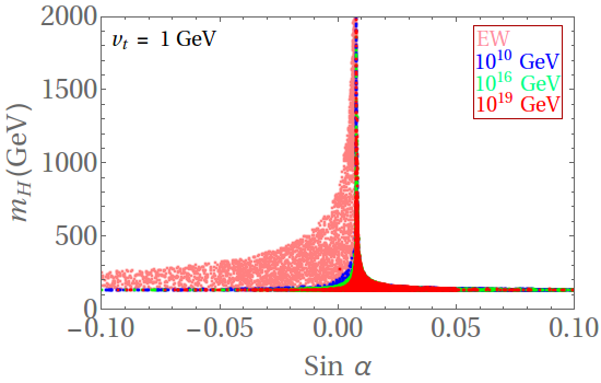
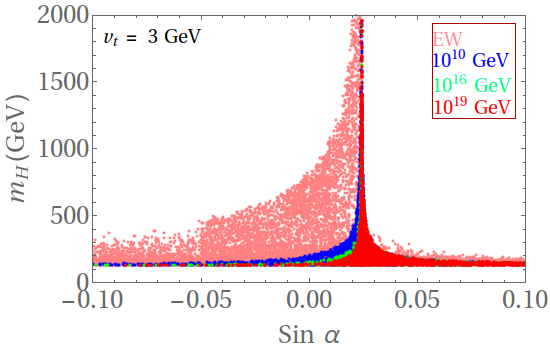
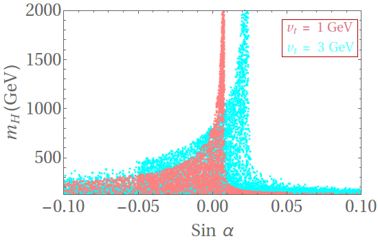
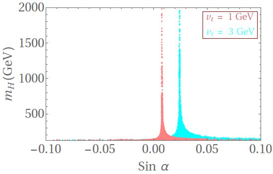
Figure 1: (Upper panel) The valid parameter space in the $\sin\alpha-m_{H}$ plane for $v_{t}=1~{}\rm GeV$ (left) and $v_{t}=3~{}\rm GeV$ (right) for different values of cut-off scale. Different colors indicate the different high cut-off scale while the background (pink) shaded region is only allowed at the EW scale. (Lower panel) The explicit distinction between the allowed parameter space by the two different $v_{t}$ valid only at the EW scale(left) and all the way up to the Planck scale(right).

Henceforth, whenever we mention a high-scale valid region we would mean the parameter space allowed by both the high-scale stability and the perturbativity constraints. This follows from the fact that the scalar quartic couplings do not feel any negative pull from fermionic loops during its running as the triplet does not couple with quarks and the lepton Yukawas are too small to consider. Therefore, the strongest constraint will come from the demand of high-scale perturbative unitarity. Although, one can always think of a model that does not respect perturbative unitarity at high scale which can call for some UV completion of the model, we restrict us from discussing this possibility in this work.

Now, as mentioned before, we have also considered a restrictive bound of 50 GeV between the singly and doubly charged scalar mass splittings, not to violate the T-parameter constraints. But, the requirement of absolute stability and unitarity actually entail a relation among the scalar mass parameters and not all of them remain independent. This is true even at the EW scale [15], however the extra demand of high-scale validity puts more stringent bound on the limits. For the sake of completeness, we would like to briefly explain the inherent nature of the parameter space due to the simultaneous stability and unitarity constraints. The conditions given in Eqs.(19a and 20f) when translated to mass terms using Eq.(18), yield the CP-odd neutral scalar mass $(m_{A})$ as a function of the two other CP-even scalar masses $(m_{h},m_{H})$ and their mixing angle $\alpha$ and can be approximated as,

$$m_{A}^{2}\simeq(m_{H}^{2}\cos^{2}\alpha+m_{h}^{2}\sin^{2}\alpha)\,$$ (22)

for $v_{t}<<v_{d}$. In the similar fashion, the doubly charged scalar mass can also be determined once we set the unitarity condition of Eq.(20j) in addition to the above which turns out to be in the close proximity of $(2m_{H^{\pm}}^{2}-m_{A}^{2})$. We did not use this mass relations for the $m_{A}^{2}$ and $m_{H^{\pm\pm}}^{2}$ to scan the parameter range instead we independently scan all the masses in the range given in Eq. (21). But, at the end, we see that the mass of $m_{A}$ and $m_{H^{\pm\pm}}$ bear such relation to maintain the stability and unitarity constraints. In the first row of Fig.1, we show the allowed region for the EW scale and the three distinct cut-off scales namely, $10^{10}\,,10^{16}~{}\&~{}10^{19}$ GeV respectively in $(\sin\alpha$-$m_{H})$ plane, where $m_{H}$ denotes the mass of heavier CP-even Higgs. It is interesting to note that significant amount of allowed parameter space at EW scale shrinks once we impose the stability of the vacuum all the way up to the Planck scale.

It is also worth noticing that the large value of the exotic scalar masses happens only for a small nonzero value of $\sin\alpha$ when high scale stability is demanded and the absolute range of $\sin\alpha$ shifts towards more positive value if the triplet vev is increased from 1 GeV to 3 GeV. This is again a consequence of the unitarity bound which can be understood by looking at Eq. (20a). The relation when translated in terms of the physical scalar masses using Eq. (18), turns out to be

$$\frac{2m_{A}^{2}}{v_{d}^{2}+4v_{t}^{2}}+\frac{\sin 2\alpha}{2v_{d}v_{t}}(m_{h}^{2}-m_{H}^{2})<16\pi\,.$$ (23)

Now, for $v_{t}<<v_{d}$ and using Eq. (22), the limit is trivially satisfied for $\sin\alpha\simeq 2v_{t}/v_{d}$ reaching the decoupling limit of large $m_{H}(>>m_{h})$. This also means that the in the SM-like limit for large $m_{H}$, the mixing angle tends to zero for $v_{t}\to 0$. Therefore, with an increase in $v_{t}$ will essentially shift the decoupling region for the non-standard scalars to larger mixing angle. This feature is reflected in Fig. 1 where the peak of the allowed region is shifted for $v_{t}=1$ to 3 GeV to more positive $\sin\alpha$. In the second row of Fig. 1, we explicitly show the shift in peak for the two different values of the $v_{t}$ in the region allowed only at the EW scale and all the way up to the Planck scale respectively.

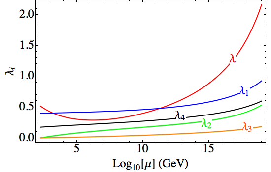
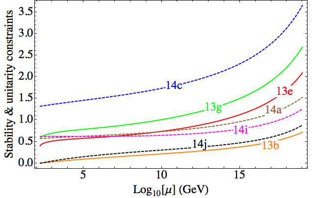
Figure 2: (Left panel) The running of the five scalar quartic couplings up to the Planck scale for the benchmark point BP1 of positive scenario as given in Table 1. (Right panel) The running of some of the stability and unitarity constraints indicated by the corresponding equation numbers for the same benchmark point.

We also show the running of individual scalar quartic coupling and some of the stability and unitarity conditions in Fig. 2 valid up to the Planck scale for a benchmark point (BP1 of positive scenario) given in Table 1.

In the next part of this paper, we shall explore the parameter space available at the Planck scale allowed region in the current LHC run and look at the prospect of some possible collider signals for the non-standard scalar particles. Accordingly, it is to be noted from Fig. 1 (upper two panels) that for large mixing angle $(\sin\alpha\sim{\cal O}({0.1}))$, a Planck scale valid region only allows the heavier neutral scalar mass $(m_{H})$ close to the lighter SM-like higgs mass $m_{h}$, namely the degenerate scenario. Moreover, the other triplet scalar masses $(m_{A},m_{H^{\pm}},m_{H^{\pm\pm}})$ are also pushed in the same mass range due to the unitarity and T-parameter constraints. However, for our collider study we only consider the non-degenerate scenario and therefore a triplet scalar masses around a few hundred GeV (200-300 GeV) instantly restrict us to a small range of mixing angle $(0.01<\sin\alpha<0.05)$ for $v_{t}=3~{}\rm GeV$ as can be seen from Fig 1.

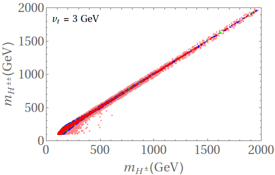
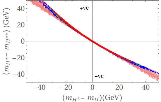
Figure 3: (Left panel) The allowed parameter space in the $m_{H^{\pm}}-m_{H^{\pm\pm}}$ plane for triplet vev $v_{t}=3~{}\rm GeV$. The different colors follow the same convention as in Fig. 1. (Right panel) The corresponding allowed parameter space to show the relation between the mass splittings of the singly charged Higgs to the neutral Higgs $(m_{H^{\pm}}-m_{H})$ and singly charged Higgs to the doubly charged Higgs $(m_{H^{\pm}}-m_{H^{\pm\pm}})$. The upper left square corresponds to the valid region for our positive scenario while the lower right corner denotes the same but for our negative scenario.

In this work, we aim to study the possible signature of charged scalar sector of the model, more specifically, we investigate the signal of the associated production of the singly and doubly charged scalars for some specific signal processes. Before going into the detail, we show the allowed parameter space in $(m_{H^{\pm}}-m_{H^{\pm\pm}})$ plane in the left panel of Fig. 3 for $v_{t}=3~{}\rm GeV$. Here, one should recall that the doubly charged mass in the high-scale stable parameter space is related to the singly charged scalar and neutral scalar mass squares as:

$$m^{2}_{H^{\pm\pm}}-m^{2}_{H^{\pm}}\approx m^{2}_{H^{\pm}}-m^{2}_{A}(m^{2}_{H})\,.$$ (24)

This yields two different scenarios depending on the mass hierarchy between the triplet scalars:

1. Positive scenario $(\lambda_{4}>0)$ :: $m_{H^{\pm\pm}}<m_{H^{\pm}}<m_{A}/m_{H}$.

2. Negative scenario $(\lambda_{4}<0)$ :: $m_{H^{\pm\pm}}>m_{H^{\pm}}>m_{A}/m_{H}$.

In fact the names are self-explanatory since the mass differences in Eq. (24) equate to $-\frac{1}{4}\lambda_{4}v_{d}^{2}$ which is obtained from Eq. (18e). Therefore, positive scenario stands for a positive $\lambda_{4}$ while the negative scenario delivers a negative $\lambda_{4}$. In the right panel of Fig. 3, we show the high-scale allowed parameter space for these two distinct mass scenarios. We shall perform the collider analysis for both mass scenarios. Now, at this point, we would like to comment that we have explicitly checked that the allowed region up to the Planck scale is consistent with the Higgs to diphoton signal strength at $2\sigma$ level.

V Collider Analysis

Following our discussion in the previous section, hereby, we address some predictive collider signal in the charged scalar sector at the current LHC run with $\sqrt{s}=13~{}\rm TeV$, in compliance with the parameter space available when the cutoff scale is set at the Planck scale. We mainly pursue the associated production of the doubly and singly charged scalar as our dominant production channel. To understand the ensuing final states at the LHC, it is thus instructive to check the decay patterns of the charged scalars in the chosen parameter space. We have mentioned earlier that at large $v_{t}\sim 3~{}\rm GeV$, the leptonic decay modes of the triplets become extremely suppressed and only decay to gauge bosons are allowed. At such value, doubly charged Higgs decay to $W^{\pm}W^{\pm}$ with almost 100% branching ratio while the singly charged scalar can have mainly three types of decay modes $(W^{\pm}Z,t\bar{b},W^{\pm}h)$ depending on the phase space available due to its mass. In Fig. 4, we show the variation of branching ratio for both the charged scalars as a function of $m_{H^{\pm}}$ and $m_{H^{\pm\pm}}$ for the mixing angle $\sin\alpha=0.02$. Here only the positive mass scenario has been depicted, the decay patterns remain unchanged for the negative scenario. We only show the mass ranges above the $W^{\pm}Z$ onshell mass threshold below which only three body decay modes are available for both singly and doubly charged scalars. Depending on the mass difference between the charged scalars either off-shell gauge boson ($W^{\pm}$ or $Z$) or off-shell charged scalar $H^{\pm\pm}$($H^{\pm}$) will be produced for positive(negative) scenarios. Therefore, we only show the mass ranges ( $>$ 170 GeV ) that allow two body decay modes of the charged scalars.

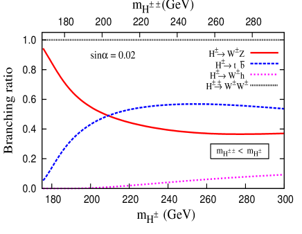
Figure 4: Branching ratio of different two body decay modes for the doubly charged and singly charged scalars for $\sin\alpha=0.02$ and $v_{t}=3~{}\rm GeV$ for the positive scenario.

For $(170-200)~{}\rm GeV$ mass range, the singly charged scalar dominantly decays into $W^{\pm}Z$ mode. On the other hand, the doubly charged scalar decays to $W^{\pm}W^{\pm}$ with 100% branching ratio due to the choice of the triplet vev ($v_{t}$). The presence of the multi gauge bosons ($W^{\pm},Z$) in the final state motivate us to consider the following two signal topologies :

$$(i) 3\ell^{\pm}+E_{T}/\;\>\,;$$

$$(ii) (\ell^{+}\ell^{+})+4j+E_{T}/\;\>\,,$$

where, $\ell=e,\mu$ and $j$ corresponds to jets (included non-tagged $b$-jets). We also include the contributions from the charge conjugated process. At this point, it is worth mentioning that the experimental searches done till date has only scrutinized the possibility of having multilepton final states from the primary decay of the doubly charged scalar probing only the lower triplet vev ( $v_{t}\leq 10^{-4}~{}\rm GeV$ ) scenario. However, those search strategies can not be applicable for the signal processes (i) and (ii) due to very different kinematics of the final state leptons which are the end product of the cascade decay of singly and doubly charged scalars. Through our detailed analysis we will show that our principal search mode for this scenario relies on the final state (ii). Here it should also be mentioned that while the final state (i) can only emerge from the associated ($pp\rightarrow H^{\pm\pm}H^{\mp}$) production process, the other final state (ii) receives contributions from both the associated ($pp\rightarrow H^{\pm\pm}H^{\mp}$) and the pair-production ($pp\rightarrow H^{++}H^{--}$) processes.

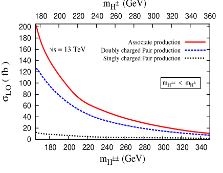
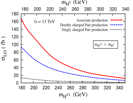
Figure 5: Left (Right) panel shows the variation of $\sigma_{\rm LO}(pp\rightarrow H^{\pm\pm}H^{\mp})~{}\rm(fb)$ (solid red curve), $\sigma_{\rm LO}(pp\rightarrow H^{++}H^{--})~{}\rm(fb)$ (blue dashed curve) and $\sigma_{\rm LO}(pp\rightarrow H^{+}H^{-})~{}\rm(fb)$ (black dotted curve) with respect to charged Higgs masses at the LHC at $\sqrt{s}=\rm 13~{}TeV$ for positive (negative) scenario.

In Fig. 5 we show the $\sigma_{\rm LO}(pp\rightarrow H^{\pm\pm}H^{\mp})$, $\sigma_{\rm LO}(pp\rightarrow H^{++}H^{--})$ and $\sigma_{\rm LO}(pp\rightarrow H^{+}H^{-})$ cross sections at the $\sqrt{s}=13~{}\rm TeV$ LHC (where LO stands for leading order). As it is very evident from these figures that the pair production rate of singly charged scalars is order of magnitude smaller than that of $H^{++}H^{--}$ and $H^{\pm\pm}H^{\mp}$ production cross-sections. Hence, for our collider study we only consider $H^{++}H^{--}$ and $H^{\pm\pm}H^{\mp}$ production processes.

Mass Scenario	$\sin\alpha$	$m_{H^{\pm\pm}}$	$m_{H^{\pm}}$	$m_{H}=m_{A}$	$\mu_{\gamma\gamma}$
		$(\rm GeV)$	$(\rm GeV)$	$(\rm GeV)$
Positive
BP1	0.0220	165.48	173.25	180.70	0.79
BP2	0.0280	175.99	177.47	178.93	0.82
Negative
BP1	0.0277	179.60	176.30	173.01	0.79
BP2	0.0300	184.17	180.11	175.95	0.81

Table 1: Benchmark points valid by the high-scale stability constraints up to the Planck scale and their corresponding Higgs to diphoton signal strength ($\mu_{\gamma\gamma}$) for both the positive and the negative scenario. The current experimental value of $\mu_{\gamma\gamma}$ is $0.85^{+0.22}_{-0.20}$ [59].

We now choose few representative benchmark points as shown in Table  1 from the region which are allowed by the stability condition all the way up to the Planck scale. We show benchmark points for both the mass hierarchies.

Along with the masses of the triplet scalar and the neutral mixing angle, we present the Higgs to diphoton signal strength ($\mu_{\gamma\gamma}$) for each benchmark points which is allowed by the $2\sigma$ limit of the current Higgs data $(0.85^{+0.22}_{-0.20})$ [59].

For our analysis, both the signal and SM backgrounds events are generated at the Leading Order (LO) parton level in Madgraph5(v2.3.3) [61] using the NNPDF3.0 parton distributions [62]. The model has been implemented in FeynRules [63] which gives the UFO model files required in madgraph. The parton showering and hadronisation is done using the built-in Pythia [64] in the madgraph. The showered events are then passed through Delphes(v3) [65] for the detector simulation where the jets are constructed using the anti-$K_{T}$ jet algorithm. For the background processes with hard jets, proper MLM matching scheme [66] has been chosen. The cut-based analyses are done using the MadAnalysis5 [67].

Several SM processes contribute as backgrounds to the aforementioned two final states. We consider the following SM processes in our analysis: $t\bar{t}$+jets (up to 3), single top with three hard jets, $V+{\rm jets~{}(up~{}to~{}3~{}jets)},V\equiv W^{\pm},Z$, $VV$+ 3 jets, $t\bar{t}+(W^{\pm}/Z/h)$, and $VVV$. As we will see, the backgrounds from top quark production can be handled using the $b$-veto while the $W^{\pm}/Z+~{}\rm jets$ and $W^{+}W^{-}+~{}\rm jets$ processes with large production cross-section can be suppressed with the three-lepton or same-sign dilepton selection criteria. Finally, the irreducible backgrounds left are the $W^{\pm}Z+~{}\rm jets$ and $t\bar{t}+(W^{\pm}/Z/h)$ with small effective cross-section. It is worthwhile to mention here that all the signal production channels are of purely electroweak type, while some of the SM background processes are either pure QCD or QCD+EW in nature with huge cross section. However, as we will show, a suitable choice of selection cuts can improve the signal significance appreciably.

In our signal and background events, we select jets and leptons using the following basic kinematical acceptance cuts :

$$\Delta R_{jj}>0.6,~{}~{}~{}~{}\Delta R_{\ell\ell}>0.4,~{}~{}~{}~{}\Delta R_{j\ell}>0.7\,,$$ (25a)

$$\Delta R_{bj}>0.7,~{}~{}~{}~{}\Delta R_{b\ell}>0.2,$$ (25b)

$$p_{T_{\rm min}}^{j}>20~{}{\rm GeV},~{}~{}~{}~{}|\eta_{j}|<5,$$ (25c)

$$p_{T_{\rm min}}^{\ell}>10~{}{\rm GeV},~{}~{}~{}~{}|\eta_{\ell}|<2.5,$$ (25d)

where $\Delta R_{xy}=\sqrt{\Delta\phi_{xy}^{2}+\Delta\eta_{xy}^{2}}$ ($x,y\equiv\ell,j,b$) and all other symbols have their usual meaning.

Our signal processes do not include any $b$-jets and therefore a veto on the $b$-tagged jets will reduce SM backgrounds with $b$-jets. Thus for the background process, a jet has been tagged as a $b$-jet abiding by the efficiency as proposed by the ATLAS collaboration [68]:

$$\epsilon_{b}=\begin{cases}0&p_{T}^{b}\leq 30~{}\rm GeV\\ 0.6&30~{}{\rm GeV}<p_{T}^{b}<50~{}{\rm GeV}\\ 0.75&50~{}{\rm GeV}<p_{T}^{b}<400~{}{\rm GeV}\\ 0.5&p_{T}^{b}>400~{}\rm GeV~{}.\end{cases}$$ (26)

Also a mistagging probability of 10% (1%) for charm-jets (light-quark and gluon jets) has been included. For the isolation of the leptons, we follow the criteria defined in Ref. [69] where the electrons are isolated with the Tight criterion defined in Ref. [70] and the muons are isolated using the Medium criterion defined in Ref. [71]

V.1 Cut-based Analysis

In this section, we first examine the aforementioned signal topologies based on different kinematic variables. Then, considering the optimal prospect, we propose some selection cuts to extract the signal from the background. Finally, we shed light on the prospect of discovering such signals at the LHC.

V.1.1 $3\ell^{\pm}+E_{T}/\;\>\,$

This final state consisting of trilepton plus missing transverse energy originates from the secondary decay of the gauge bosons produced from the decay of the charged scalars. For a particular charge assignment, the final state is developed as

$$pp\to H^{++}H^{-}\to(W^{+}W^{+})+(W^{-}Z)\to(\ell^{+}\ell^{+})+\ell^{-}+E_{T}/\;\>\,.$$ (27)

Even though this signal also encases a pair of same-sign lepton, the presence of the third lepton hinders the process of selection. Before detailing the selection cuts, let us first discuss the distributions of some of the relevant kinematic variables used in the signal selection procedure. All the distributions are normalized to respective cross section of the process and for the background distribution, we only show the irreducible background processes. One more important point to note that we do not enforce the leptonic decay mode for the SM $W^{\pm}$ and $Z$ rather we consider the all inclusive decay channels for both the signal and background event generation. This is true for all the subsequent analyses.

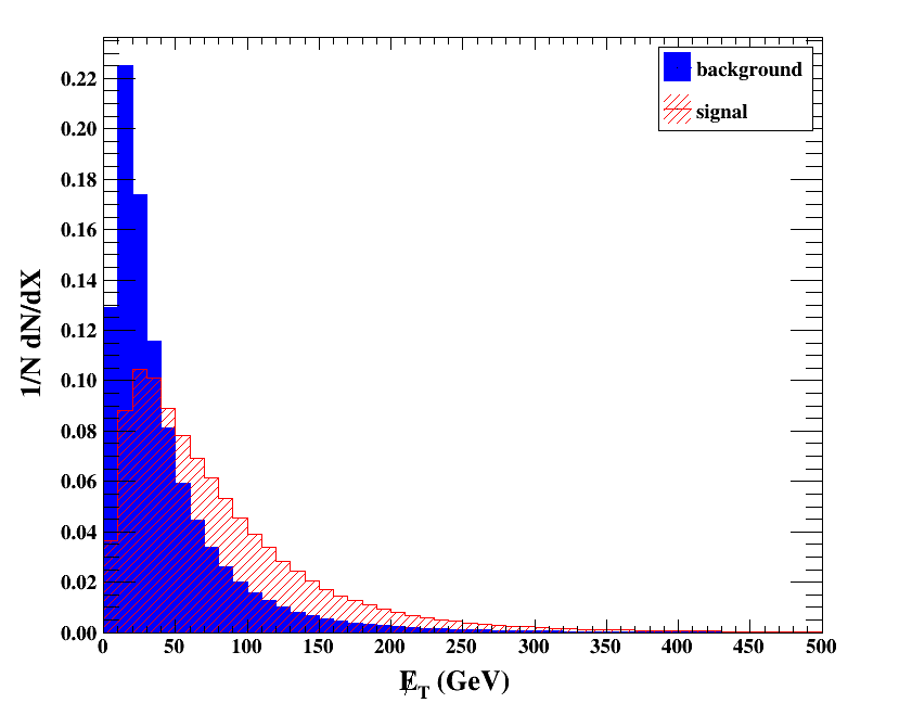
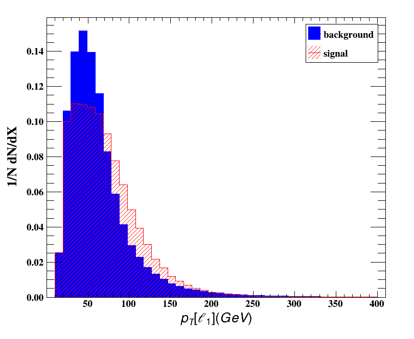
Figure 6: Normalized distribution of the (left panel) Missing transverse energy $(E_{T}/\;\>)$ and (right panel) the transverse momentum of the hardest lepton $(p_{T}(\ell_{1}))$ after the basic kinematical acceptance cuts for the benchmark BP1 of positive scenario.

We start with the missing transverse energy ($E_{T}/\;\>$) distribution, depicted in the left panel of Fig. 6 for the benchmark point (BP1) of the positive scenario with highest production cross-section. Since the decay pattern for the negative scenario does not change, therefore we do not show the same for that scenario. To explicate the nature of the distribution, we remind that the $E_{T}/\;\>$  for both the signal and the backgrounds originates solely from neutrinos (from $Z$ and $W^{\pm}$ decays). As a consequence, the overall nature of the histogram for the signal and background events looks similar except a slight deviation at the peak. The background events (blue dark shaded area) peak at lower $E_{T}/\;\>$ $(\lesssim 30$ GeV) compared to our signal events. This is just an imprint of the slight boost in the gauge boson transverse momentum due to the heavier parent particles ( $H^{\pm\pm}$ and $H^{\pm}$). Hence, a requirement of $E_{T}/\;\>>30$ GeV may be effective for a good signal to background ratio.

In the right panel of Fig. 6, we show the transverse momentum ($p_{T}$) distributions of the hardest ($p_{T}$ ordered) lepton for the same benchmark while in Fig. 7, we draw the transverse momentum distribution for the other two sub-leading leptons. Again, for both the signal and background events, these three leptons come from the SM gauge boson decay except with a little smearing effect for the signal distribution due to its origin from heavier particles. Therefore, it is quite difficult to put a selection cut on these three leptons to disentangle the signal and background and we can only put the basic acceptance cut to the three leptons to assure a trilepton signature and veto on any additional fourth lepton. However, one interesting fact is that the two opposite sign leptons emanate from two different gauge bosons. This suggests that an invariant mass cut on the same flavor opposite-sign lepton around the $Z$ boson mass shall surely reduce a large number of background events from $W^{\pm}/Z+\rm jets$, $ZZ+\rm jets$ and $W^{\pm}Z+\rm jets$. In addition to this, since the signal is free from any additional jet, a jet veto instantly cut down the giant background processes.

As already mentioned, the important feature of both of our signal processes is the presence of a pair of same-sign lepton, a claim of which can largely suppress the SM background. In this endeavor we define another kinematic variable, the angular separation $\Delta R(\ell^{\pm}\ell^{\pm})$ between the two same-sign leptons. The distribution is featured in Fig. 8. For our signal events, both these same-sign leptons come from the same-sign $W^{\pm}$ bosons which are produced from the decay of single heavy doubly charged scalar $H^{\pm\pm}$. The same-sign charged leptons tend to appear at small opening angle due to the spin correlation between the parent $W^{\pm}W^{\pm}$ pair [72, 73]. As a result, the $\Delta R(\ell^{\pm}_{1}\ell^{\pm}_{2})$ distribution peaks at a relatively lower value. On the other hand, same-sign leptons from all the background events would have much wider separation as they originate directly from $W^{\pm}/Z$ bosons that are either produced as a pair of primary objects or are radiated from top/anti-top quark. Thus, an upper cut on the $\Delta R(\ell_{1}^{\pm}\ell_{2}^{\pm})(<1.5)$ considerably enhances our signal to background ratio. However, since the signal distribution do not show a steeply falling nature, this cut would also reduce the number of detectable signal events.

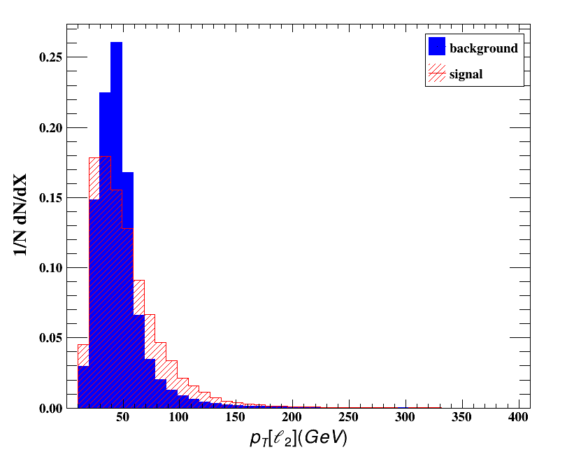
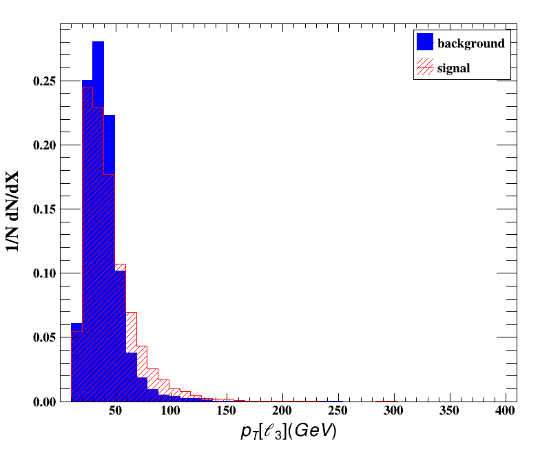
Figure 7: Transverse momentum $(p_{T})$ distribution (normalized) of the two sub-leading leptons for the benchmark BP1 of positive scenario.

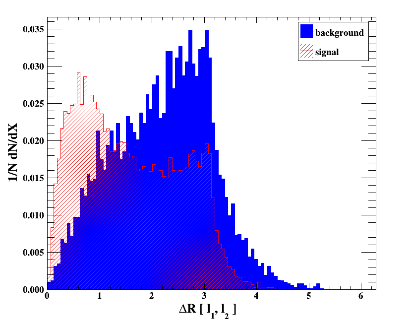
Figure 8: The $\Delta R(\ell_{1}^{\pm}\ell_{2}^{\pm})$ distribution (normalized) between the two same-sign leptons for the positive scenario benchmark BP1.

A summary of all these cuts is as follows:

• (C1-1): Our signal event is hadronically quiet, hence, we put a veto on any jet with $p_{T}>30$ GeV. From Table 2, it can be understood that the reduction in signal events is only the aftermath of branching ratio suppression for the gauge boson decay. On the contrary, all the SM backgrounds with accompanying jets receive significant cutback in total cross section.

• (C1-2): Next, to confirm the trilepton signature, we select at least three leptons with $p_{T}>10$ GeV. This cut essentially removes most of the backgrounds arising from these SM processes: $t+$ jets, $t\bar{t}+$ jets, $W^{\pm}+$ jets, $Z+$ jets, $W^{+}W^{-}+$ jets with less number of isolated leptons, also evident from Table 2.

• (C1-3): For further affirmation of trilepton signature, we reject any additional charged lepton with $p_{T}>10$ GeV. This, however, does not play a crucial role rather serves as a systematic attestation.

• (C1-4): Furthermore, we claim that the same flavour opposite sign (SFOS) lepton invariant mass ${\rm M}_{\ell^{+}\ell^{-}}$ should not lie between the window of 80-100 GeV to ensure that those are not directly produced from $Z$ boson. This helps in suppressing the two most important background, i.e. $ZZ+\rm jets$ and $W^{\pm}Z+\rm jets$.

• (C1-5): For missing energy requirement, we demand $E_{T}/\;\>>30$ GeV.

• (C1-6): The principal selection cut for the same-sign dilepton has been imposed. For this, we demand $\Delta R(\ell^{\pm}_{1}\ell^{\pm}_{2})<$ 1.5.

In Table 2, we compile the effect of the aforementioned cuts for both the signal (for all four benchmark points corresponding to both positive and negative scenario) and the SM background events and calculate the signal significance defined as

$${\mathscr{S}}=\frac{N_{S}}{\sqrt{N_{S}+N_{B}}}\,,$$ (28)

where, $N_{S}(N_{B})$ denotes the number of signal (background) events at a specific luminosity.

		Effective cross section (fb) for background after the cut
SM-background	Production Cross section (fb)	C1–1	C1–2	C1–3	C1–4	C1–5	C1–6
$t$+jets	$2.22\times 10^{5}$	157.50	0	0	0	0	0
$t\bar{t}$+jets	$7.07\times 10^{5}$	420.37	0	0	0	0	0
$W^{\pm}$+jets	$1.54\times 10^{8}$	$4.96\times 10^{7}$	0	0	0	0	0
$Z$+jets	$4.54\times 10^{7}$	$1.37\times 10^{7}$	0	0	0	0	0
$W^{+}W^{-}$+jets	$8.22\times 10^{4}$	$4.76\times 10^{3}$	0	0	0	0	0
$ZZ$+jets	$1.10\times 10^{4}$	$6.17\times 10^{2}$	10.05	5.77	0.08	0.04	$\sim$ 0
$W^{\pm}Z$+jets	$3.81\times 10^{4}$	$1.71\times 10^{3}$	42.40	42.40	0.72	0.36	0.04
$W^{+}W^{-}Z$	83.10	1.17	0.09	0.07	0.01	$\sim$ 0	0
$W^{\pm}ZZ$	26.80	0.39	0.03	0.03	$\sim$ 0	0	0
$t\bar{t}+W^{\pm}$	360	0.13	0.02	$\sim$ 0	0	0	0
$t\bar{t}+Z$	585	0.15	0.02	0.01	$\sim$ 0	0	0
$t\bar{t}+h$	400	0.02	$\sim$ 0	0	0	0	0
Total SM Background	$2.005\times 10^{8}$	$6.33\times 10^{7}$	52.60	48.30	0.81	0.40	0.04
Positive scenario	Production Cross section (fb)	Effective cross section (fb) for signal after the cut						Luminosity (in $\rm fb^{-1}$) for 5$\sigma$ significance
BP1	185.10	0.75	0.20	0.14	0.08	0.06	0.040	1250.0
BP2	158.70	0.65	0.16	0.11	0.06	0.05	0.034	1600.4
Negative scenario	Production Cross section (fb)	Effective cross section (fb) for signal after the cut						Luminosity (in $\rm fb^{-1}$) for 5$\sigma$ significance
BP1	153.80	0.63	0.16	0.11	0.06	0.05	0.033	1675.8
BP2	134.70	0.55	0.15	0.10	0.05	0.04	0.030	1944.4

Table 2: Effective cross section obtained after each cut for both signal ($3\ell^{\pm}+E_{T}/\;\>\,\,$) and background and the respective required integrated luminosity for 5$\sigma$ significance at $\rm 13~{}TeV$ LHC.

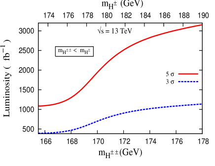
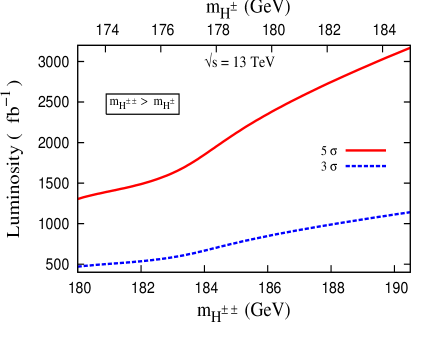
Figure 9: Left (Right) panel shows the required integrated luminosity for $3\ell^{\pm}+E_{T}/\;\>\,$ final state with respect to charged Higgs masses at the LHC at $\sqrt{s}=\rm 13~{}TeV$ for positive (negative) scenario. The solid red coloured and blue coloured dashed curve correspond to constant signal significance at 5$\sigma$ and 3$\sigma$ respectively.

In Fig. 9, we show the required luminosity at 13 TeV LHC run to reach signal significance $5\sigma$ (red solid curve) and $3\sigma$(blue dashed curve) respectively for a range of singly and doubly charged scalar mass for both the positive and negative scenarios. It is evident from the figure that a $5\sigma$ discovery reach at the 13 TeV LHC run can be achieved both in the positive and negative scenario with a minimum integrated luminosity of $1250{~{}\rm fb}^{-1}$, even if the charged scalar masses lie at the ballpark of 170 GeV.

For the negative scenario, the required luminosity is a little higher due to the phase space suppression as the mass of the doubly charged scalar is higher than that of the singly charged scalar. Therefore, the model prediction can only be probed through this channel with a High Luminosity LHC (HL-LHC) run.

Before concluding this section, we would like to comment that there can be two more signal topologies, namely: (a)$5\ell^{\pm}+E_{T}/\;\>$ and (b) $3\ell^{\pm}+4j+E_{T}/\;\>\,$. However, the effective cross section for channel (a) is suppressed by a factor of 3 due to the fact that $\frac{BR(Z\to\ell^{+}\ell^{-})}{BR(Z\to\nu\nu)}\sim\frac{1}{3}$. Moreover, due to the occurrence of two same-sign di-lepton, one arising from secondary decay of the doubly charged scalars while the other from that of the singly charged scalar, the angular separation cut will not be very helpful. In addition to that, since the $Z$ boson decays to charged lepton final state, we can not impose cut C1-4 in this case. We have checked that to attain $5\sigma$ signal significance we need at least $\sim 3100~{}{\rm fb^{-1}}$ luminosity, which can only be probed with very high luminosity run of the LHC.
Coming to the second topology, i.e. the $3\ell^{\pm}+4j+E_{T}/\;\>\,$ channel, the effective cross-section is 4 times larger than the $3\ell^{\pm}+E_{T}/\;\>\,$ channel. In spite of that larger cross-section the significance is much lesser due to the fact the $W^{\pm}Z+~{}{\rm jets}$ SM background mimics the signal and also the angular separation cut is not effective as mentioned before. As a result, we require minimum $2350~{}{\rm fb^{-1}}$ luminosity to reach $5\sigma$ significance.

V.1.2 $2\ell^{\pm}+4j+E_{T}/\;\>$

This particular channel receives contributions from both doubly charged pair production $(H^{++}H^{--})$ and singly charged scalar associated with doubly charged scalar production $(H^{\pm\pm}H^{\mp})$ processes. The decay chains which lead to this final state are depicted by:

$$pp\to H^{++}H^{--} \to (W^{+}W^{+})+(W^{-}W^{-})\to(\ell^{+}\ell^{+})+4j+E_{T}/\;\>\,~{},$$ (29a)

$$pp\to H^{++}H^{-} \to (W^{+}W^{+})+(W^{-}Z)\to(\ell^{+}\ell^{+})+4j+E_{T}/\;\>~{}.$$ (29b)

The other charge combination should also be included. The LSD nature of this final state makes it a very promising channel to explore the Type II seesaw scenario at the LHC. In addition to the LSD, the signal channel also contains four hard jets and a moderate amount of missing transverse energy.

Before we embark our study of selection cuts on different kinematic variables associated with this signal channel, we would like to discuss the general features of this final state. The LSDs originate from the decays of two same-signed $W^{\pm}$ bosons. Here, we expect that the transverse momentum $(p_{T})$ spectrum of these leptons would be very similar to those charged leptons of our previous channel simply because of their identical origin, the $W^{\pm}$ boson. The neutrinos produced in association with the charged leptons from the decay of $W^{\pm}$ bosons are the main source of the observed $E_{T}/\;\>$. However, there is a small contribution to it which comes from the uncertainty associated with jet energy measurement. We expect that the $E_{T}/\;\>$  distribution would not be very different from that of the previous channel, as displayed in the left panel of Fig. 6.

In Fig. 10, we show the $p_{T}$ distributions of the four hardest jets for both the signal and the background events. By looking at the shape of the jet $p_{T}$ distributions, it is very clear that the signal jets are relatively harder than that of the SM backgrounds. This can attributed to the fact that for the signal process, these jets originate from the decays of different $W^{\pm}$ and $Z$ bosons which in turn produced with some transverse momentum from the decay of heavy $H^{\pm}$ and $H^{\pm\pm}$ Higgs bosons. On the other hand significant fraction of the SM background jets originate from the initial state of final state radiation, making them relatively softer compared to the signal jets. So, we demand that our signal events should have four jets starting from a leading jet with $p_{T}(j_{1})>60$ GeV and subsequently, the next to leading jet with $p_{T}(j_{2})>40$ GeV while the rest of the jets with at least $p_{T}>20$ GeV are asked. However, these jets do not originate from $b$-quark hadronisation and so a veto on $b$-tagged jet is extremely useful in increasing the signal significance.

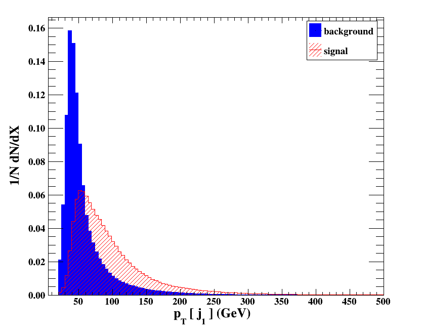
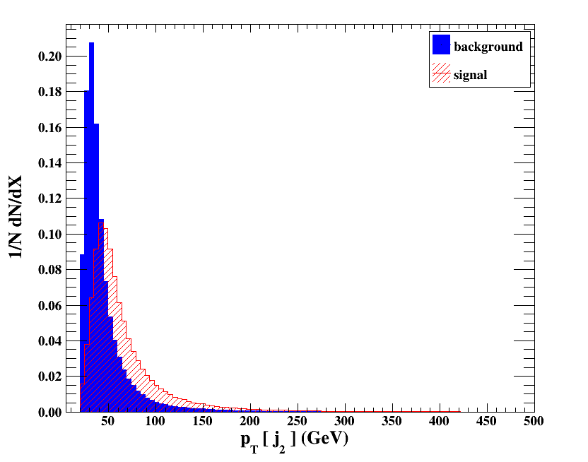
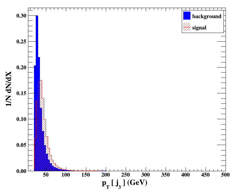
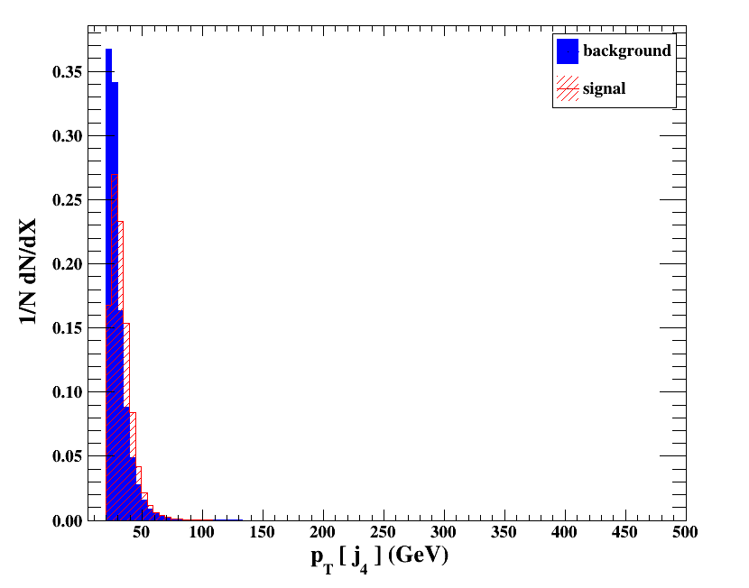
Figure 10: Transverse momentum $(p_{T})$ distribution (normalized) of the four leading jets for the final state $2\ell^{\pm}+4j+E_{T}/\;\>$ for the benchmark BP1 of positive scenario.

Akin to our previous case, the distribution of the angular separation $\Delta R(\ell^{\pm}\ell^{\pm})$ between the two same-sign leptons follows the same nature as shown in Fig. 8. However, in this signal channel absence of any additional charged lepton makes the cut more severe to the background with respect to the signal. We will see that an upper cut on the $\Delta R(\ell_{1}^{\pm}\ell_{2}^{\pm})(<1.5)$ helps gaining a huge signal significance.

Following the general features of the distributions of different kinematical variables, we now implement our selection criteria :

• (C2-1): As explained, our signal is exempted from any $b$-jets, hence we can safely reject events with $b$-tagged jets of $p_{T}(b)>40$ GeV. This cut drastically reduces the SM background events arising from $t\bar{t}+\rm jets$, $t+\rm jets$ and $t\bar{t}$+$(h/W^{\pm}/Z)$ processes.

• (C2-2): To guarantee that only 4 jets are present in the events, we reject any additional jets with $p_{T}(j_{5})>20$ GeV.

• (C2-3): Our signal also contains two isolated charged lepton and thus a veto on any additional leptons with $p_{T}>10$ GeV is applied.

• (C2-4): Now, from the jet distribution, we choose the $p_{T}$ of the leading jet to be at least greater than $p_{T}(j_{1})>60$ GeV. This helps in a modest drop in background events.

• (C2-5): Moreover, for the next sub-leading jet we demand $p_{T}(j_{2})>40$ GeV to further subdue the background events.

• (C2-6): A decent selection cut on the missing transverse energy is then applied as $E_{T}/\;\>>30$ GeV.

• (C2-7): At the end, we demand $\Delta R(\ell^{\pm}_{1}\ell^{\pm}_{2})<$ 1.5 as the most effective cut. We find that this cut is crucial for achieving higher signal significance.

We list the gradual effect of the selection cuts on the signal and background events in Table 3. We estimate the required integrated luminosity (using the Eq. (28)) to observe a $5\sigma$ significance corresponding to each benchmark points for both the scenarios at the 13 TeV LHC. It is evident from Table 3 that this signal can even be observed with a $5\sigma$ significance with only a mere $27~{}\rm fb^{-1}$ luminosity for the benchmark point of highest cross-section. For the rest of the benchmark also the required luminosity is quite low (30-50 $\rm fb^{-1}$). Hence, we may expect to see this final state at $5\sigma$ signal significance at the current run of the 13 TeV LHC.

		Effective cross section (fb) after the cut
SM-background	Production Cross section (fb)	C2–1	C2–2	C2–3	C2–4	C2–5	C2–6	C2–7
$t$+jets	$2.22\times 10^{5}$	$8.46\times 10^{4}$	$8.01\times 10^{4}$	$8.01\times 10^{4}$	$4.89\times 10^{4}$	$3.44\times 10^{4}$	$1.54\times 10^{4}$	0
$t\bar{t}$+jets	$7.07\times 10^{5}$	$1.58\times 10^{5}$	$1.23\times 10^{5}$	$1.23\times 10^{5}$	$9.92\times 10^{4}$	$8.15\times 10^{4}$	$5.58\times 10^{4}$	0
$W^{\pm}$+jets	$1.54\times 10^{8}$	$1.52\times 10^{8}$	$1.52\times 10^{8}$	$1.52\times 10^{8}$	$1.24\times 10^{7}$	$8.17\times 10^{6}$	$1.75\times 10^{6}$	0
$Z$+jets	$4.54\times 10^{7}$	$4.27\times 10^{7}$	$4.27\times 10^{7}$	$4.27\times 10^{7}$	$3.76\times 10^{6}$	$2.48\times 10^{6}$	$4.65\times 10^{5}$	0
$W^{+}W^{-}$+jets	$8.22\times 10^{4}$	$7.84\times 10^{4}$	$7.55\times 10^{4}$	$7.55\times 10^{4}$	$3.48\times 10^{4}$	$2.39\times 10^{4}$	$1.04\times 10^{4}$	0
$ZZ$+jets	$1.10\times 10^{4}$	$8.96\times 10^{3}$	$8.67\times 10^{3}$	$8.65\times 10^{3}$	$4.27\times 10^{3}$	$2.89\times 10^{3}$	$1.16\times 10^{3}$	0.05
$W^{\pm}Z$+jets	$3.81\times 10^{4}$	$3.33\times 10^{4}$	$3.13\times 10^{4}$	$3.12\times 10^{4}$	$1.67\times 10^{4}$	$1.18\times 10^{4}$	$5.76\times 10^{3}$	1.68
$t\bar{t}+W^{\pm}$	360	78.00	55.15	55.00	47.00	39.80	33.00	0.13
$t\bar{t}+Z$	585	110.00	68.20	67.00	59.60	52.04	44.30	0.04
$t\bar{t}+h$	400	46.00	27.40	27.20	24.50	21.65	18.30	0.04
Total SM Background	$2.005\times 10^{8}$	$1.95\times 10^{8}$	$1.94\times 10^{8}$	$1.94\times 10^{8}$	$1.64\times 10^{7}$	$1.08\times 10^{7}$	$2.31\times 10^{6}$	1.94
Positive scenario	Production Cross section (fb)	Effective cross section (fb) for signal after the cut							Luminosity (in $\rm fb^{-1}$) for 5$\sigma$ significance
BP1	311.40	253.00	210.70	206.70	181.72	158.90	126.24	1.90	26.6
BP2	259.30	211.23	175.92	172.64	151.75	132.66	105.42	1.55	36.3
Negative scenario	Production Cross section (fb)	Effective cross section (fb) for signal after the cut							Luminosity (in $\rm fb^{-1}$) for 5$\sigma$ significance
BP1	246.23	200.00	166.50	163.32	143.61	125.54	99.76	1.50	38.2
BP2	219.30	177.74	148.03	145.22	127.70	111.63	88.71	1.30	47.9

Table 3: Effective cross section obtained after each cut for both signal ($2\ell^{\pm}+4j+E_{T}/\;\>$) and background and the respective required integrated luminosity for 5$\sigma$ significance at $\rm 13~{}TeV$ LHC.

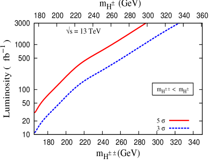
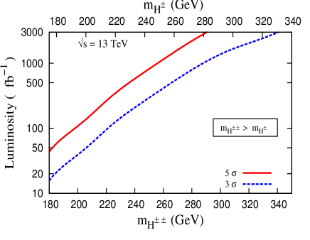
Figure 11: Left (Right) panel shows the required integrated luminosity for $2\ell^{\pm}+4j+E_{T}/\;\>$ final state with respect to charged Higgs masses at the LHC at $\sqrt{s}=\rm 13~{}TeV$ for positive (negative) scenario. The solid red coloured and blue coloured dashed curve correspond to constant signal significance at 5$\sigma$ and 3$\sigma$ respectively.

After obtaining a very encouraging signal to background ratio for this channel, we now try to get an estimate of the singly and doubly charged Higgs mass range which the 13 TeV LHC can probe and the integrated luminosity required for this purpose. In Fig. 11 we show the $3\sigma$ and $5\sigma$ significance contour in the mass of heavy charged scalar ($m_{H^{\pm\pm}}$ (lower axis) and $m_{H^{\pm}}$ (upper axis)) and integrated luminosity plane for positive (left) and negative (right) scenarios respectively. One can see that running at 13 TeV energy and with the 3 ${\rm ab}^{-1}$ integrated luminosity the LHC can probe the singly(doubly) charged scalar masses up to 300(280) GeV and up to 335(320) GeV with 5$\sigma$ and 3$\sigma$ significance for the positive scenario (left panel of Fig. 11). For the negative scenario (right panel of Fig. 11), the LHC reach is almost identical with the positive scenario except with a reverse mass hierarchy between the singly and doubly charged scalars. It is also very clear that for the masses around 200 GeV, the integrated luminosity of about a 100 $\rm fb^{-1}$ is more than sufficient to get the discovery reach of 5$\sigma$. We thus strongly motivate this channel to be looked at the current run of the LHC.

In passing, we would like to comment that the channel $(\ell^{+}\ell^{-})+4j+E_{T}/\;\>$ has same effective cross section as our second signal process. But absence of a pair of same sign lepton plague the detection of this channel. Even with $3~{}{{\rm ab}^{-1}}$ luminosity, only $1\sigma$ significance can be achieved.

Before making our conclusion, we would like to stress that while estimating signal significances for both the channels we have not taken into account different the experimental issues arising from the electron charge misidentification, jet faking as leptons and photon conversions into lepton pair. However, we have found that the misidentification probability of a jet to be an isolated electron is around $(0.1-0.2)\%$ for $p_{T}\simeq 30~{}\rm GeV$ for the Tight criterion [70]. This would imply that for the $3\ell+E_{T}/\;\>~{}~{}{\rm and}~{}2\ell+4j+E_{T}/\;\>~{}\rm$ signal channels, all the SM multi-jet background processes will be down by order $10^{-9}$ and $10^{-6}$ respectively. The electron misidentification probability is also very small $({\cal O}(0.1\%))$ in the central rapidity region [74]. As far as the photon conversions into $e^{+}e^{-}$ probability is concerned, we expect it to be of similar level as other two aforementioned fake rates. One should note that our search result is independent of the mass hierarchy of the charged scalars and appear to be equally discernible at the LHC. Also, we strongly motivate the same-sign dilepton plus jets and missing energy channel as an aspiring search channel at the current LHC run.

VI Conclusion

With an intention to solve the infamous vacuum instability problem, we have recalled the Type-II seesaw model where the SM scalar sector is extended with an $SU(2)_{L}$ triplet scalar. We have found that the additional scalar fields can certainly surmount the instability problem and provide us with an absolutely stable vacuum even up to the Planck scale. The stipulation of the stability, unitarity and T-parameter constraints altogether up to the high cut-off scale severely affect the allowed model parameter space favored at the EW scale. To exemplify, we have chosen two distinct values of the triplet vev $v_{t}$ (1 and 3 GeV) and show the amount of parameter space spared by the above theoretical constraints. We have observed that the requirement of an absolutely stable vacuum up to the high Planck scale have pushed the neutral scalar mixing angle $(\alpha)$ to a quite small range of value for the non-degenerate mass scenario $(m_{H}(m_{A})\gg m_{h})$ and peaks around a small positive value for considerably large $m_{H}$. The peak shifted to a more positive value with increasing $v_{t}$. On the other hand, the mass differences among all the other non-standard scalar masses have narrowed down to small values. Besides an almost degenerate non-standard CP-even ($H$) and CP-odd ($A$) neutral scalar, the doubly and singly charged scalars also become closer in mass.

Next, we have inspected the expectancy to detect the model prediction, available from high-scale valid scenario, at the current and high luminosity run of the LHC. We have particularly investigated the associated production of the singly and doubly charged scalars. Depending on the mass hierarchy, two possible scenarios (positive and negative) exist which however, at the end, yielded similar signal significance. In the allowed parameter space, with appreciable production cross section, the masses of the charged scalar can presumably be chosen around 200 GeV. This mass choice along with our choice of triplet vev, fix the possible decay modes of the charged scalars. Correspondingly it give rises to two specific final states at the collider, ($3\ell^{\pm}+E_{T}/\;\>\,$) and $(2\ell^{\pm}+4j+E_{T}/\;\>)$ at the 13 TeV LHC run. A proper cut-based analysis with detector simulation reveals that the first channel can only be probed at the 13 TeV LHC with high integrated luminosity around 1250 $\rm fb^{-1}$ and should be promoted for a HL-LHC. On the other hand, the second signal channel has better observability at the 13 TeV LHC due to larger production rate and better cut efficiencies. We have found that even a $5\sigma$ discovery reach is possible with the present LHC data with only around $40~{}\rm fb^{-1}$ luminosity. We would like to mention that our estimation of the signal significance is based on simple cut based analysis, where we did not include some experimental issues arising from jet faking as leptons, lepton charge misidentification and photon conversions into lepton pairs. We have argued semi-quantitatively that the first two fake rates would not affect our main conclusions and expect that the photon conversions into lepton pairs would also be rather small. Any quantitative statements regarding aforementioned fake rates are beyond the scope of this phenomenological analysis. We agree that the proper inclusion of these fake rates as well as systematic uncertainties in the SM background estimation would certainly modify the signal significance quoted in this paper, hence our conclusions may be considered as an indicative one. We hope that the results presented in this paper would encourage the experimental collaborations to perform more dedicated analysis in this direction to probe this scenario both in the current and future run of the LHC.

VII Acknowledgement

N.G. and A.S. would like to thank Subhadeep Mondal for useful discussions. N.G. would like to acknowledge the Council of Scientific and Industrial Research (CSIR), Government of India for financial support. We all are thankful to Subir Sarkar and Manas Maity for useful discussions.

Appendix

Appendix A One loop RG equations

Here, we will present the one loop RGEs of all the relevant couplings (gauge, Yukawa and scalar quartic couplings) of the Type-II seesaw model [60, 75]. For convenience, we introduce the shorthand notation ${\cal D}\equiv 16\pi^{2}\frac{\rm d}{\rm{d(ln\mu)}}$.

Gauge and top Yukawa couplings:

The RGE for the gauge couplings,

$${\cal D}g_{1} = \frac{47}{10}{g_{1}}^{3}\,,$$ (30a)

$${\cal D}g_{2} = -\frac{5}{2}g_{2}^{3}\,,$$ (30b)

$${\cal D}g_{3} = -7g_{3}^{3}\,.$$ (30c)

The RGE for the top Yukawa coupling,

$${\cal D}y_{t} = y_{t}\left(\frac{9}{2}y_{t}^{2}-\left(8g_{3}^{2}+\frac{9}{4}g_{2}^{2}+\frac{17}{20}{g_{1}}^{2}\right)\right)\,,$$ (30d)

where, $g_{1}=\sqrt{\frac{5}{3}}g^{\prime}$ with GUT renormalization. The boundary values of the gauge couplings at $M_{Z}$ are taken to be [46]

$$g_{1}(M_{Z}) = \sqrt{\frac{5}{3}}0.3569\,,\qquad g_{2}(M_{Z})=0.6531\,,\qquad g_{3}(M_{Z})=\sqrt{4\pi 0.1185}\,.$$ (31)

While the boundary condition for the top Yukawa interaction at the electroweak scale is fixed by $y_{t}(M_{t})=\frac{\sqrt{2}m_{t}(M_{t})}{v}$. For the matching condition between the $\overline{MS}$ mass of top quark to its pole mass, we consider the dominant one-loop QCD correction as $m_{t}(M_{t})\sim M_{t}\left(1-\frac{4}{3\pi}\alpha_{s}(M_{t})\right)$, $M_{t}$ being the top pole mass fixed at 173 GeV throughout the analysis and the strong coupling $\alpha_{s}(M_{t})$ is derived from the gauge coupling running from $M_{Z}$ to $M_{t}$.

Scalar quartic couplings:

We express the RGEs of the scalar quartic coupling with a redefinition of the coupling to match with the potential notation of Ref. [75] which can be translated from our notation in the following way.

$$\Lambda_{0} = \frac{\lambda}{2}\,,$$ (32a)

$$\Lambda_{1} = 2\lambda_{2}+2\lambda_{3}\,,$$ (32b)

$$\Lambda_{2} = -2\lambda_{3}\,,$$ (32c)

$$\Lambda_{4} = \lambda_{1}+\frac{\lambda_{4}}{2}\,,$$ (32d)

$$\Lambda_{5} = -\frac{\lambda_{4}}{2}\,.$$ (32e)

The RGEs for the five quartic couplings that appear are then given by,

$${\cal D}\Lambda_{i}=\beta_{\Lambda_{i}}+G_{i}\,,(i=0,1,2,4,5)\,,$$ (33)

where, $\beta_{\Lambda_{i}}$ and $G_{i}$ are as follows:

$$\beta_{\Lambda_{0}} = 12\Lambda_{0}^{2}+6\Lambda_{4}^{2}+4\Lambda_{5}^{2}\,,$$ (34a)

$$\beta_{\Lambda_{1}} = 14\Lambda_{1}^{2}+4\Lambda_{1}\Lambda_{2}+2\Lambda_{2}^{2}+4\Lambda_{4}^{2}+4\Lambda_{5}^{2}\,,$$ (34b)

$$\beta_{\Lambda_{2}} = 3\Lambda_{2}^{2}+12\Lambda_{1}\Lambda_{2}-8\Lambda_{5}^{2}\,,$$ (34c)

$$\beta_{\Lambda_{4}} = \Lambda_{4}\left(8\Lambda_{1}+2\Lambda_{2}+6\Lambda_{0}+4\Lambda_{4}+8\Lambda_{5}^{2}\right)\,,$$ (34d)

$$\beta_{\Lambda_{5}} = \Lambda_{5}\left(2\Lambda_{1}-2\Lambda_{2}+2\Lambda_{0}+8\Lambda_{4}\right)\,,$$ (34e)

and,

$$G_{0} = \left(12y_{t}^{2}-\left(\frac{9}{5}g_{1}^{2}+9g_{2}^{2}\right)\right)\Lambda_{0}+\frac{9}{4}\left(\frac{3}{25}g_{1}^{4}+\frac{2}{5}g_{1}^{2}g_{2}^{2}+g_{2}^{4}\right)-12y_{t}^{4}\,,$$ (35a)

$$G_{1} = -\left(\frac{36}{5}g_{1}^{2}+24g_{2}^{2}\right)\Lambda_{1}+\frac{108}{25}g_{1}^{4}+18g_{2}^{4}+\frac{72}{5}g_{1}^{2}g_{2}^{2}\,,$$ (35b)

$$G_{2} = -\left(\frac{36}{5}g_{1}^{2}+24g_{2}^{2}\right)\Lambda_{2}+12g_{2}^{4}-\frac{144}{5}g_{1}^{2}g_{2}^{2}\,,$$ (35c)

$$G_{4} = \left(6y_{t}^{2}-\left(\frac{9}{2}g_{1}^{2}+\frac{33}{2}g_{2}^{2}\right)\right)\Lambda_{4}+\frac{27}{25}g_{1}^{4}+6g_{2}^{4}\,,$$ (35d)

$$G_{5} = \left(6y_{t}^{2}-\left(\frac{9}{2}g_{1}^{2}+\frac{33}{2}g_{2}^{2}\right)\right)\Lambda_{5}-\frac{18}{5}g_{1}^{2}g_{2}^{2}\,.$$ (35e)

References

- [1] ATLAS collaboration, G. Aad et al., Observation of a new particle in the search for the Standard Model Higgs boson with the ATLAS detector at the LHC, Phys. Lett. B716 (2012) 1–29, [1207.7214].
- [2] CMS collaboration, S. Chatrchyan et al., Observation of a new boson at a mass of 125 GeV with the CMS experiment at the LHC, Phys. Lett. B716 (2012) 30–61, [1207.7235].
- [3] J. Elias-Miro, J. R. Espinosa, G. F. Giudice, G. Isidori, A. Riotto and A. Strumia, Higgs mass implications on the stability of the electroweak vacuum, Phys. Lett. B709 (2012) 222–228, [1112.3022].
- [4] G. Degrassi, S. Di Vita, J. Elias-Miro, J. R. Espinosa, G. F. Giudice, G. Isidori et al., Higgs mass and vacuum stability in the Standard Model at NNLO, JHEP 08 (2012) 098, [1205.6497].
- [5] S. Alekhin, A. Djouadi and S. Moch, The top quark and Higgs boson masses and the stability of the electroweak vacuum, Phys. Lett. B716 (2012) 214–219, [1207.0980].
- [6] F. Bezrukov, M. Yu. Kalmykov, B. A. Kniehl and M. Shaposhnikov, Higgs Boson Mass and New Physics, JHEP 10 (2012) 140, [1205.2893].
- [7] I. Masina, Higgs boson and top quark masses as tests of electroweak vacuum stability, Phys. Rev. D87 (2013) 053001, [1209.0393].
- [8] D. Buttazzo, G. Degrassi, P. P. Giardino, G. F. Giudice, F. Sala, A. Salvio et al., Investigating the near-criticality of the Higgs boson, JHEP 12 (2013) 089, [1307.3536].
- [9] E. J. Chun, H. M. Lee and P. Sharma, Vacuum Stability, Perturbativity, EWPD and Higgs-to-diphoton rate in Type II Seesaw Models, JHEP 11 (2012) 106, [1209.1303].
- [10] W. Chao, M. Gonderinger and M. J. Ramsey-Musolf, Higgs Vacuum Stability, Neutrino Mass, and Dark Matter, Phys. Rev. D86 (2012) 113017, [1210.0491].
- [11] P. S. Bhupal Dev, D. K. Ghosh, N. Okada and I. Saha, 125 GeV Higgs Boson and the Type-II Seesaw Model, JHEP 03 (2013) 150, [1301.3453].
- [12] N. Haba, H. Ishida, N. Okada and Y. Yamaguchi, Vacuum stability and naturalness in type-II seesaw, Eur. Phys. J. C76 (2016) 333, [1601.05217].
- [13] P. S. B. Dev, C. M. Vila and W. Rodejohann, Naturalness in testable type II seesaw scenarios, Nucl. Phys. B921 (2017) 436–453, [1703.00828].
- [14] M. Chabab, M. C. Peyranère and L. Rahili, Naturalness in a type II seesaw model and implications for physical scalars, Phys. Rev. D93 (2016) 115021, [1512.07280].
- [15] D. Das and A. Santamaria, Updated scalar sector constraints in the Higgs triplet model, Phys. Rev. D94 (2016) 015015, [1604.08099].
- [16] J. Schechter and J. W. F. Valle, Neutrino Masses in SU(2) x U(1) Theories, Phys. Rev. D22 (1980) 2227.
- [17] M. Magg and C. Wetterich, Neutrino Mass Problem and Gauge Hierarchy, Phys. Lett. 94B (1980) 61–64.
- [18] T. P. Cheng and L.-F. Li, Neutrino Masses, Mixings and Oscillations in SU(2) x U(1) Models of Electroweak Interactions, Phys. Rev. D22 (1980) 2860.
- [19] G. Lazarides, Q. Shafi and C. Wetterich, Proton Lifetime and Fermion Masses in an SO(10) Model, Nucl. Phys. B181 (1981) 287–300.
- [20] R. N. Mohapatra and G. Senjanovic, Neutrino Masses and Mixings in Gauge Models with Spontaneous Parity Violation, Phys. Rev. D23 (1981) 165.
- [21] M. Lindner, M. Platscher and F. S. Queiroz, A Call for New Physics : The Muon Anomalous Magnetic Moment and Lepton Flavor Violation, 1610.06587.
- [22] G. ’t Hooft, Naturalness, chiral symmetry, and spontaneous chiral symmetry breaking, NATO Sci. Ser. B 59 (1980) 135–157.
- [23] P. F. de Salas, D. V. Forero, C. A. Ternes, M. Tortola and J. W. F. Valle, Status of neutrino oscillations 2017, 1708.01186.
- [24] Gfitter Group collaboration, M. Baak, J. Cúth, J. Haller, A. Hoecker, R. Kogler, K. Mönig et al., The global electroweak fit at NNLO and prospects for the LHC and ILC, Eur. Phys. J. C74 (2014) 3046, [1407.3792].
- [25] A. Arhrib, R. Benbrik, M. Chabab, G. Moultaka and L. Rahili, Higgs boson decay into 2 photons in the type II Seesaw Model, JHEP 04 (2012) 136, [1112.5453].
- [26] M. Carena, I. Low and C. E. M. Wagner, Implications of a Modified Higgs to Diphoton Decay Width, JHEP 08 (2012) 060, [1206.1082].
- [27] M. Aoki, S. Kanemura, M. Kikuchi and K. Yagyu, Radiative corrections to the Higgs boson couplings in the triplet model, Phys. Rev. D87 (2013) 015012, [1211.6029].
- [28] P. Fileviez Perez, T. Han, G.-y. Huang, T. Li and K. Wang, Neutrino Masses and the CERN LHC: Testing Type II Seesaw, Phys. Rev. D78 (2008) 015018, [0805.3536].
- [29] A. Melfo, M. Nemevsek, F. Nesti, G. Senjanovic and Y. Zhang, Type II Seesaw at LHC: The Roadmap, Phys. Rev. D85 (2012) 055018, [1108.4416].
- [30] M. Aoki, S. Kanemura and K. Yagyu, Testing the Higgs triplet model with the mass difference at the LHC, Phys. Rev. D85 (2012) 055007, [1110.4625].
- [31] ATLAS collaboration, T. A. collaboration, Search for doubly-charged Higgs boson production in multi-lepton final states with the ATLAS detector using proton-proton collisions at , ATLAS-CONF-2017-053 (2017) .
- [32] A. G. Akeroyd and M. Aoki, Single and pair production of doubly charged Higgs bosons at hadron colliders, Phys. Rev. D72 (2005) 035011, [hep-ph/0506176].
- [33] A. G. Akeroyd and C.-W. Chiang, Doubly charged Higgs bosons and three-lepton signatures in the Higgs Triplet Model, Phys. Rev. D80 (2009) 113010, [0909.4419].
- [34] A. G. Akeroyd and C.-W. Chiang, Phenomenology of Large Mixing for the CP-even Neutral Scalars of the Higgs Triplet Model, Phys. Rev. D81 (2010) 115007, [1003.3724].
- [35] A. G. Akeroyd and H. Sugiyama, Production of doubly charged scalars from the decay of singly charged scalars in the Higgs Triplet Model, Phys. Rev. D84 (2011) 035010, [1105.2209].
- [36] C.-W. Chiang, T. Nomura and K. Tsumura, Search for doubly charged Higgs bosons using the same-sign diboson mode at the LHC, Phys. Rev. D85 (2012) 095023, [1202.2014].
- [37] S. Kanemura, K. Yagyu and H. Yokoya, First constraint on the mass of doubly-charged Higgs bosons in the same-sign diboson decay scenario at the LHC, Phys. Lett. B726 (2013) 316–319, [1305.2383].
- [38] Z. Kang, J. Li, T. Li, Y. Liu and G.-Z. Ning, Light Doubly Charged Higgs Boson via the Channel at LHC, Eur. Phys. J. C75 (2015) 574, [1404.5207].
- [39] S. Kanemura, M. Kikuchi, K. Yagyu and H. Yokoya, Bounds on the mass of doubly-charged Higgs bosons in the same-sign diboson decay scenario, Phys. Rev. D90 (2014) 115018, [1407.6547].
- [40] S. Kanemura, M. Kikuchi, H. Yokoya and K. Yagyu, LHC Run-I constraint on the mass of doubly charged Higgs bosons in the same-sign diboson decay scenario, PTEP 2015 (2015) 051B02, [1412.7603].
- [41] C.-H. Chen and T. Nomura, Search for with new decay patterns at the LHC, Phys. Rev. D91 (2015) 035023, [1411.6412].
- [42] Z.-L. Han, R. Ding and Y. Liao, LHC Phenomenology of Type II Seesaw: Nondegenerate Case, Phys. Rev. D91 (2015) 093006, [1502.05242].
- [43] Z.-L. Han, R. Ding and Y. Liao, LHC phenomenology of the type II seesaw mechanism: Observability of neutral scalars in the nondegenerate case, Phys. Rev. D92 (2015) 033014, [1506.08996].
- [44] M. Mitra, S. Niyogi and M. Spannowsky, Type-II Seesaw Model and Multilepton Signatures at Hadron Colliders, Phys. Rev. D95 (2017) 035042, [1611.09594].
- [45] A. Arhrib, R. Benbrik, M. Chabab, G. Moultaka, M. C. Peyranere, L. Rahili et al., The Higgs Potential in the Type II Seesaw Model, Phys. Rev. D84 (2011) 095005, [1105.1925].
- [46] Particle Data Group collaboration, C. Patrignani et al., Review of Particle Physics, Chin. Phys. C40 (2016) 100001.
- [47] C. Bonilla, J. C. Romão and J. W. F. Valle, Electroweak breaking and neutrino mass: ‘invisible’ Higgs decays at the LHC (type II seesaw), New J. Phys. 18 (2016) 033033, [1511.07351].
- [48] C. Bonilla, R. M. Fonseca and J. W. F. Valle, Consistency of the triplet seesaw model revisited, Phys. Rev. D92 (2015) 075028, [1508.02323].
- [49] L. Lavoura and L.-F. Li, Making the small oblique parameters large, Phys. Rev. D49 (1994) 1409–1416, [hep-ph/9309262].
- [50] OPAL, DELPHI, L3, ALEPH, LEP Higgs Working Group for Higgs boson searches collaboration, Search for charged Higgs bosons: Preliminary combined results using LEP data collected at energies up to 209-GeV, in Lepton and photon interactions at high energies. Proceedings, 20th International Symposium, LP 2001, Rome, Italy, July 23-28, 2001, 2001, hep-ex/0107031, http://weblib.cern.ch/abstract?CERN-L3-NOTE-2689.
- [51] ATLAS collaboration, G. Aad et al., Search for charged Higgs bosons through the violation of lepton universality in events using collision data at TeV with the ATLAS experiment, JHEP 03 (2013) 076, [1212.3572].
- [52] CMS collaboration, S. Chatrchyan et al., Search for a light charged Higgs boson in top quark decays in collisions at TeV, JHEP 07 (2012) 143, [1205.5736].
- [53] M. Spira, HIGLU: A program for the calculation of the total Higgs production cross-section at hadron colliders via gluon fusion including QCD corrections, hep-ph/9510347.
- [54] ATLAS collaboration, T. A. collaboration, Search for ZZ resonances in the final state in pp collisions at = 13 TeV with the ATLAS detector, ATLAS-CONF-2016-016 (2016) .
- [55] ATLAS collaboration, M. Aaboud et al., Search for heavy resonances decaying into in the final state in collisions at TeV with the ATLAS detector, Eur. Phys. J. C78 (2018) 24, [1710.01123].
- [56] F. Arbabifar, S. Bahrami and M. Frank, Neutral Higgs Bosons in the Higgs Triplet Model with nontrivial mixing, Phys. Rev. D87 (2013) 015020, [1211.6797].
- [57] S. Kanemura and K. Yagyu, Radiative corrections to electroweak parameters in the Higgs triplet model and implication with the recent Higgs boson searches, Phys. Rev. D85 (2012) 115009, [1201.6287].
- [58] A. G. Akeroyd and S. Moretti, Enhancement of H to gamma gamma from doubly charged scalars in the Higgs Triplet Model, Phys. Rev. D86 (2012) 035015, [1206.0535].
- [59] ATLAS collaboration, T. A. collaboration, Measurement of fiducial, differential and production cross sections in the decay channel with 13.3 fb-1 of 13 TeV proton-proton collision data with the ATLAS detector, ATLAS-CONF-2016-067 (2016) .
- [60] W. Chao and H. Zhang, One-loop renormalization group equations of the neutrino mass matrix in the triplet seesaw model, Phys. Rev. D75 (2007) 033003, [hep-ph/0611323].
- [61] J. Alwall, R. Frederix, S. Frixione, V. Hirschi, F. Maltoni, O. Mattelaer et al., The automated computation of tree-level and next-to-leading order differential cross sections, and their matching to parton shower simulations, JHEP 07 (2014) 079, [1405.0301].
- [62] NNPDF collaboration, R. D. Ball et al., Parton distributions for the LHC Run II, JHEP 04 (2015) 040, [1410.8849].
- [63] A. Alloul, N. D. Christensen, C. Degrande, C. Duhr and B. Fuks, FeynRules 2.0 - A complete toolbox for tree-level phenomenology, Comput. Phys. Commun. 185 (2014) 2250–2300, [1310.1921].
- [64] T. Sjostrand, S. Mrenna and P. Z. Skands, PYTHIA 6.4 Physics and Manual, JHEP 05 (2006) 026, [hep-ph/0603175].
- [65] DELPHES 3 collaboration, J. de Favereau, C. Delaere, P. Demin, A. Giammanco, V. Lemaître, A. Mertens et al., DELPHES 3, A modular framework for fast simulation of a generic collider experiment, JHEP 02 (2014) 057, [1307.6346].
- [66] S. Hoeche, F. Krauss, N. Lavesson, L. Lonnblad, M. Mangano, A. Schalicke et al., Matching parton showers and matrix elements, in HERA and the LHC: A Workshop on the implications of HERA for LHC physics: Proceedings Part A, pp. 288–289, 2005, hep-ph/0602031, DOI.
- [67] E. Conte, B. Fuks and G. Serret, MadAnalysis 5, A User-Friendly Framework for Collider Phenomenology, Comput. Phys. Commun. 184 (2013) 222–256, [1206.1599].
- [68] ATLAS collaboration, T. A. collaboration, Calibration of the performance of -tagging for and light-flavour jets in the 2012 ATLAS data, ATLAS-CONF-2014-046 (2014) .
- [69] ATLAS collaboration, T. A. collaboration, Measurement of the production cross section in collisions at a centre-of-mass energy of TeV with the ATLAS experiment, ATLAS-CONF-2016-090 (2016) .
- [70] ATLAS collaboration, T. A. collaboration, Electron efficiency measurements with the ATLAS detector using the 2015 LHC proton-proton collision data, ATLAS-CONF-2016-024 (2016) .
- [71] ATLAS collaboration, G. Aad et al., Muon reconstruction performance of the ATLAS detector in proton–proton collision data at =13 TeV, Eur. Phys. J. C76 (2016) 292, [1603.05598].
- [72] M. Dittmar and H. K. Dreiner, How to find a Higgs boson with a mass between 155-GeV - 180-GeV at the LHC, Phys. Rev. D55 (1997) 167–172, [hep-ph/9608317].
- [73] M. Dittmar and H. K. Dreiner, as the Dominant SM Higgs search mode at the LHC for GeV, in The Higgs puzzle - what can we learn from LEP-2, LHC, NLC and FMC? Proceedings, Ringberg Workshop, Tegernsee, Germany, December 8-13, 1996, pp. 113–121, 1996, hep-ph/9703401.
- [74] CMS collaboration, V. Khachatryan et al., Performance of Electron Reconstruction and Selection with the CMS Detector in Proton-Proton Collisions at √s = 8 TeV, JINST 10 (2015) P06005, [1502.02701].
- [75] M. A. Schmidt, Renormalization group evolution in the type I+ II seesaw model, Phys. Rev. D76 (2007) 073010, [0705.3841].